Two-loop master integrals for a planar topology contributing to $pp\rightarrow t\bar{t}j$

Abstract

We report on recent progress for the QCD corrections to top quark pair plus jet production. In particular, we discuss a recent computation for the two-loop master integrals associated to a two-loop five-point pentagon-box integral configuration with one internal massive propagator, that contributes to top quark pair production in association with a jet in the QCD planar limit.

1 Introduction

The Large Hadron Collider (LHC) is entering the high-precision era with the High-Luminosity plan (HI-LHC). This project will enable experimental collaborations to measure many interesting observables at percent level precision. In order to be able to compare the experimental measurements with theoretical predictions, it is mandatory to achieve a theoretical uncertainty on the same level of the experimental one. One of the ingredients that are needed in order to achieve this goal are next-to-next-to leading order (NNLO) QCD corrections. While a lot progress has been done recently in this framework, QCD corrections at NNLO are still not available for all the most interesting observables at LHC.

One of the observables for which NNLO QCD corrections are yet to be obtained is the top quark pair production in association with a jet. As the top quark is the heaviest particle in the Standard Model (SM) of particle physics, it has many important implications for the nature of the fundamental forces. In particular many properties of the SM are sensitive to the value of the top quark mass as, for example, the stability of the SM vacuum whose precision measurement is a high priority at the (LHC). The standard process which is exploited to measure the top quark mass at the LHC is top quark pair production. This process is known with vey high precision both theoretically and experimentally [1, 2]. However, it has been recently argued that top quark pair production in association with a jet is even more sensitive to the top quark mass [3, 4, 5]. The state-of-the-art for the theoretical predictions of this process is represented by the next-to-leading order (NLO) QCD corrections [6, 7], along with complete decay information and interfaces with a parton shower [8, 9, 10, 11, 12]. However, in order to match the experimental precision, see for example [13, 14], next-to-next-to-leading order (NNLO) corrections are required.

In order to be able to perform a full NNLO prediction for this observable several computational difficulties have to be overcome. One of the major obstacles is the computation of the required two-loop scattering amplitudes. Recently a great progress has been made in the calculation of scattering amplitudes for $2\to 3$ processes [15, 16, 17, 18, 19, 20, 21, 22, 23, 24, 25, 26, 27, 28, 29, 30, 31, 32, 33, 34], which led to a number of NNLO QCD theoretical predictions [35, 36, 37, 38, 39, 40]. Yet, the amplitudes necessary to perform a NNLO theoretical prediction for top quark pair plus a jet production at LHC represent a substantial step forward with respect to the current state-of-the-art. Indeed, the top quark mass which appear in the internal propagators is responsible for a significant growth in the complexity of the computation. This feature affect both the algebraic complexity in the amplitude reconstruction, and the analytic complexity of the Feynman integrals.

In this context, I report on the recent progress made in the computation of two-loop Feynman integrals relevant for the NNLO QCD corrections to $pp\to t{\bar{t}}j$ [41]. This project builds upon previous work where the authors computed the one-loop helicity amplitudes expanded up to $\mathcal{O}({\varepsilon}^{2})$ in the dimensional regulator [42], which are needed for the NNLO correections. In [41] the authors studied the master integrals associated to a five-point pentagon-box topology with one internal massive propagator, that contributes to top-quark pair production in association with a jet in the leading color QCD planar limit. The computation represents a step forward in complexity with respect to the five-point massless [15, 43, 44, 17, 45, 46] and one off-shell external leg cases [47, 48, 49, 50, 51].

The master integrals have been computed exploiting the differential equation method [52, 53]. The system of differential equations has been written with respect to a canonical basis of master integrals [54]. A major bottleneck for this computation is the solution of a large system of Integration-by-Parts (IBP) relations [55, 56]. In order to overcome this issue finite fields arithmetic [57, 58, 59], as implemented in the FiniteFlow library [59], has been employed. We obtained a semi-analytic solution for the master integrals through the generalised power series method [60, 61, 62], as described in [62] and implemented in the Mathematica package DiffExp [63]. In order to solve the system of differential equations semi-analytically, we used high precision numerical boundary conditions obtained by means of the Mathematica package AMFlow [64], which implements the auxiliary mass flow method [65, 66, 67]. Finally, we also derived the analytic representation of the alphabet for the system of differential equations. Interestingly, the structure of the alphabet has the same analytic structure as in the five-point massless [15] and in the one-mass [47] cases.

The outcome of the work presented in [41], and summarised in the present proceeding, is two-fold. First, we obtained a solution for the master integrals under study which has the potential for phenomenological applications, as it has been done for other processes [68, 69, 70, 47, 71, 50, 72, 73, 42, 74]. Moreover, the study of the analytic structure of the alphabet solution is a fundamental step in order to achieve a complete analytic representation. As a consequence, the work presented in [41] represents a fist step toward an analytic computation for the NNLO QCD corrections to top quark pair production in association with a jet in the QCD leading color planar limit.

2 Summary of the computation

We considered the pentagon-box Feynman integral topology in $d=4-2{\varepsilon}$ dimensions as shown in figure 1. This can be written as,

$$I_{a_{1},a_{2},a_{3},a_{4},a_{5},a_{6},a_{7},a_{8}}^{a_{9},a_{10},a_{11}}=\int\mathcal{D}^{d}k_{1}\mathcal{D}^{d}k_{2}\frac{D_{9}^{a_{9}}D_{10}^{a_{10}}D_{11}^{a_{11}}}{D_{1}^{a_{1}}\cdots D_{8}^{a_{8}}}\,$$ (1)

where $a_{1},\cdots,a_{11}\geq 0$. The topology is defined by the following set of propagators, and numerators:

$$D_{1} =k_{1}^{2}, D_{2} =(k_{1}-p_{1})^{2}-m_{t}^{2}, D_{3} =(k_{1}-p_{1}-p_{2})^{2},$$

$$D_{4} =(k_{1}-p_{1}-p_{2}-p_{3})^{2}, D_{5} =k_{2}^{2}, D_{6} =(k_{2}-p_{5})^{2},$$

$$D_{7} =(k_{2}-p_{4}-p_{5})^{2}, D_{8} =(k_{1}+k_{2})^{2}, D_{9} =(k_{1}+p_{5})^{2},$$

$$D_{10} =(k_{2}+p_{1})^{2}-m_{t}^{2}, D_{11} =(k_{2}+p_{1}+p_{2})^{2},$$ (2)

and the integration measure is:

$$\mathcal{D}^{d}k_{i}=\dfrac{d^{d}k_{i}}{i\pi^{\frac{d}{2}}}e^{{\varepsilon}\gamma_{E}}\,.$$ (3)

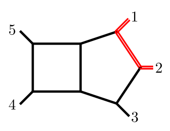
Figure 1: The pentagon-box topology contributing to $pp\rightarrow t\bar{t}j$ in the QCD leading color planar limit. Black lines denote massless particles and red double-lines denote massive particles.

The momenta are considered outgoing from the graphs and the particles are on-shell, i.e. $p_{1}^{2}=p_{2}^{2}=m_{t}^{2}$ for the top quark external legs, while $p_{3}^{2}=p_{4}^{2}=p_{5}^{2}=0$. The kinematics of the integrals is described by six independent invariants $\vec{x}=\{d_{12},d_{23},d_{34},d_{45},d_{15},m_{t}^{2}\}$, where

$$d_{ij}=p_{i}\cdot p_{j},$$ (4)

and $m_{t}^{2}$ is the top quark squared mass. After performing IBP reduction [56, 75], as implemented in the software LiteRed [76, 77] and FiniteFlow [59], we found a total number of 88 MIs (see [41] for the complete list).

We wrote a system of differential equations for the MIs $\vec{\mathcal{I}}(\vec{x},{\varepsilon})$ in canonical form [54]:

$$d\,\vec{\mathcal{I}}(\vec{x},{\varepsilon})={\varepsilon}\,dA(\vec{x})\,\vec{\mathcal{I}}(\vec{x},{\varepsilon}),$$ (5)

where $d$ is the total differential with respect to the kinematic invariants, and the matrix $A(\vec{x})$ is a linear combination of logarithms:

$$A(\vec{x})=\sum c_{i}\log(w_{i}(\vec{x})).$$ (6)

The $c_{i}$ are matrices of rational numbers, and the alphabet $\left\{w_{i}(\vec{x})\right\}$ is made by algebraic functions of the kinematic invariants $\vec{x}$.

2.1 Canonical Basis

The canonical basis of MIs $\vec{\mathcal{I}}$ has been constructed starting from the observation of an emerging pattern for $2\to 3$ scattering amplitudes [15, 43, 78, 18, 79, 45, 17, 80, 47, 50, 48]. This feature implies that we are able to rely on a good set of uniform trascendental (UT) candidate MIs as starting point for the basis construction. Specifically, one can test candidates from the MIs basis for the massless and one-mass five-point [44, 45, 47, 50] (for e.g. $pp\to W+2j$ and $pp\to 3j$) cases, as well as other integral topologies which involve internal massive propagators.

Guided by this initial set of data, our approach relies on the possibility to perform IBP reduction and evaluate the differential equations matrix over finite fields. Due to the presence of square roots, we do not attempt to construct the canonical form directly. Instead we search for a linear form, with respect to ${\varepsilon}$, which contains only rational matrices in the kinematic invariants. Indeed, the square roots appearing in the UT basis can be absorbed in the normalisation of the integral basis, and therefore we can neglect them while evaluating the differential equations over finite fields. The strategy adopted in [41] can be then summarised as follows:

• Given a starting set of UT candidate MIs, we study the ${\varepsilon}$ structure of the differential equations from a univariate slice reconstruction. Specifically, we search for a linear form in ${\varepsilon}$

  $$d\,\vec{\mathcal{J}}(\vec{x},{\varepsilon})=\,d\,\left(\hat{A}^{(0)}(\vec{x})+{\varepsilon}\widehat{A}^{(1)}(\vec{x})\right)\,\vec{\mathcal{J}}(\vec{x},{\varepsilon}),$$ (7)

  where $\widehat{A}^{(0)}$ is a diagonal matrix;

• We study the homogenous part of the system of differential equations sector-by-sector, in order to determine the correct normalisation for the MIs;

• If the starting choice of integral basis, for a given sector, does not satisfies a differential equations of the form in Eq. (7), we make a different ansatz based on criteria described below.

Once the whole system of differential equations is in the form of Eq. (7) we can rotate it into canonical form:

$$\mathcal{I}_{i}=N_{ij}(\vec{x})\mathcal{J}_{j},$$ (8)

where $N_{ij}(\vec{x})$ is a diagonal matrix which contains the square roots of the kinematic invariants. Such matrix satisfies the differential equation:

$$\widehat{A}^{(0)}-\frac{1}{2}N^{2}dN^{(-2)}=0.$$ (9)

The canonical form of the differential equations can then be written as:

$$d\,\vec{\mathcal{I}}(\vec{x},{\varepsilon})={\varepsilon}d\left(N(\vec{x})\widehat{A}^{(1)}(\vec{x})N^{-1}(\vec{x})\right)\,\vec{\mathcal{I}}(\vec{x},{\varepsilon})$$ (10)

As anticipated, if the starting integral basis does not satisfies a differential equations of the form in Eq. (7) we change the starting ansatz. This is done accordingly to a set of criteria inspired by patterns observed in previously studied cases:

• For two and three external legs MIs the choice of candidates can involve scalar integrals with dotted denominators;

• For four external legs MIs the choice of candidates can involve scalar integrals with dotted denominators or the numerators $D_{9},D_{10},D_{11}$;

• For five external legs, canonical MIs candidates can involve scalar integrals with the numerators $D_{9},D_{10},D_{11}$ and local integrand insertions $\mu_{ij}$,

where $\mu_{ij}$ are defined from the splitting of the loop momenta into four dimensional and $(-2{\varepsilon})$ dimensional components,

$$k_{i} =k_{i}^{[4]}+k_{i}^{[-2{\varepsilon}]}, \mu_{ij} =-k_{i}^{[-2\epsilon]}\cdot k_{j}^{[-2\epsilon]}.$$ (11)

I conclude the present discussion with some remarks. First, given the high number of kinematic invariants, and the large size of the IBPs systems to solve, it is important to ensure that the maximum numerator rank and number of dotted propagators is minimised. As second remark, I mention that the method exploited to build a canonical basis might still require some work on the sub-topologies contribution to the differential equations for a given sector. Indeed, we found that some sectors required additional rotations in sub-sectors. However, this step was particularly simple in our cases. Interestingly, such feature did not appear in any of the most complicated five-point topologies, where the UT integrals can be constructed exploiting just local numerator insertions.

2.2 Analytic structure

Even though the system of differential equations has been integrate semi-analytically exploiting the generalised series expansion method, we studied the alphabet structure of the solution. This aspect is crucial for understanding the analytic solution and it is the first step towards constructing a well defined special function basis for the set of MIs under consideration.

The system of differential equations can be written in terms of d-logarithmic forms using an alphabet which is made of 71 letters $w_{i}$:

$$d\,\vec{\mathcal{I}}(\vec{x},{\varepsilon})={\varepsilon}\,dA(\vec{x})\,\vec{\mathcal{I}}(\vec{x},{\varepsilon}),\,\,\,A(\vec{x})=\sum_{i=1}^{71}c_{i}\log(w_{i}(\vec{x})).$$ (12)

In order to identify the alphabet we adopted a strategy along the lines of the one described in Refs. [82, 83, 84], which we briefly summarise. As first step we identify the set of rational letters inside the alphabet. This can be done by looking at the denominators in the differential equations system. The remaining letters are, therefore, algebraic in the kinematic invariants (i.e. they contain square roots). To obtain this set of letters we proceed as follows. We determine the linear relations in the total derivative matrix $dA(\vec{x})$ and we find a minimal set of independent one forms. Then, for each independent entry of the derivative matrix one determines which square roots appear in the denominators. Finally, it is possible to construct an ansatz using free polynomials in the variables $d_{ij}$ which depends on the square roots in the one-form under study. The form of the ansatz depends on the number of square roots, e.g. if there is just one square root we can use an ansatz of the kind,

$$\Omega(a,b):=\frac{a+\sqrt{b}}{a-\sqrt{b}},$$ (13)

and in the case of two square roots,

$$\tilde{\Omega}(a,b,c):=\frac{(a+\sqrt{b}+\sqrt{c})(a-\sqrt{b}-\sqrt{c})}{(a+\sqrt{b}-\sqrt{c})(a-\sqrt{b}+\sqrt{c})}.$$ (14)

While it is always possible to expand the form of Eq. (14) into one similar to Eq. (13), the structure in Eq. (14) is preferable. Indeed, the polynomial degree of the unknown variable $a$ is lower as noted in Ref. [47].

Following this strategy we have identified an alphabet which can be split into two subsets, $\mathbf{W}_{R}$ and $\mathbf{W}_{A}$, which are, respectively, rational and algebraic in the kinematic invariants. For the rational letters we define,

$$\mathbf{W}_{R}:=\mathbf{W}_{K}\cup\mathbf{W}_{T}\cup\mathbf{W}_{S},$$ (15)

and for the algebraic letters

$$\mathbf{W}_{A}:=\mathbf{W}_{SR-1}\cup\mathbf{W}_{TR}\cup\mathbf{W}_{SR-2}.$$ (16)

The rational set of letters $\mathbf{W}_{R}$ can be furthermore divided into three subsets. The subset $\mathbf{W}_{K}$ is made by letters which are linear combinations of the Mandelstam variables $s_{ij}=(p_{i}+p_{j})^{2}$. The letters in the subset $\mathbf{W}_{T}$ can be written as traces over $\gamma$-matrices:

$$\operatorname{tr}(ij\cdots k) =\operatorname{tr}(\not{p}_{i}\not{p}_{j}\cdots\not{p}_{k}).$$ (17)

Finally, the rational letters in the third subset, $\mathbf{W}_{S}$, are related to the roots that appear in the differential equations system:

$$\mathbf{W}_{S}:= \left\{\beta^{2},\,(\Delta_{1})^{2},\,(\Delta_{2})^{2},\,4(d_{12}+d_{23}+m_{t}^{2})^{2}(\Delta_{3})^{2},\,(\Delta_{5})^{2},\,(\Delta_{4})^{2},\,(\Delta_{6})^{2},\,\operatorname{tr}_{5}^{2}\right\},$$ (18)

which are defined as follows:

$$\beta =\sqrt{1-\frac{4m_{t}^{2}}{s_{12}}},$$

$$\Delta_{1} =\sqrt{\operatorname{det}G(p_{23},p_{1})}, \Delta_{2}=\sqrt{\operatorname{det}G(p_{15},p_{2})},$$

$$\Delta_{3} =\sqrt{1-\frac{4s_{45}m_{t}^{2}}{(s_{12}+s_{23}-m_{t}^{2})^{2}}}, \Delta_{4}=\sqrt{1+\frac{4s_{34}s_{45}m_{t}^{2}}{s_{12}(s_{15}-s_{23})^{2}}},$$

$$\Delta_{5} =\sqrt{1-\frac{s_{45}m_{t}^{2}}{4d_{15}d_{23}}}, \Delta_{6}=\sqrt{1-\frac{s_{34}s_{45}m_{t}^{2}}{4d_{15}d_{23}s_{12}}},$$

$$\operatorname{tr}_{5} =4\sqrt{\operatorname{det}G(p_{3},p_{4},p_{5},p_{1})}={\rm tr}(\gamma_{5}\not{p}_{3}\not{p}_{4}\not{p}_{5}\not{p}_{1}),$$ (19)

where $G_{ij}(\vec{v})=v_{i}\cdot v_{j}$ is the Gram matrix.

Similarly to the rational subset of letters, also the algebraic one $\mathbf{W}_{A}$ can be split into three subsets. The first one, $\mathbf{W}_{SR-1}$, contains letters which can be written in terms of the quantity $\Omega$ as defined above in Eq. (13). Instead, the letters associated to the subset $\mathbf{W}_{TR}$, contain dependence on the Dirac $\gamma_{5}$ matrix. Therefore, they can be written as ratios of $\operatorname{tr}_{\pm}(ij\cdots k)$ objects, defined as

$$\operatorname{tr}_{\pm}(ij\cdots k)=\frac{1}{2}\operatorname{tr}((1\pm\gamma_{5})\not{p}_{i}\not{p}_{j}\cdots\not{p}_{k}).$$ (20)

The final subset, $\mathbf{W}_{SR-2}$, is made by letters in terms of $\tilde{\Omega}$ as defined above in Eq. (14).

I finish this discussion we the following consideration. The alphabet structure just presented shows a similar pattern to the ones observed in other five-particle kinematic configurations [85, 44, 47, 50]. This feature suggests that it might exists a general alphabet structure for all polylogarihmic two-loop integrals with five or fewer legs.

2.3 Numerical Evaluation

In order to validate our work we exploited the package DiffExp [63] to evaluate numerically the MIs. This package implements the generalised power series method [62], which gives a semi-analytical solution to the system of differential equations as an expansion around its singular points:

$$\vec{\mathcal{I}}(t,\epsilon)=\sum_{k=0}^{\infty}\epsilon^{k}\sum_{i=0}^{N-1}\rho_{i}(t)\vec{\mathcal{I}}^{(k)}_{i}(t),\;\;\;\rho(t)=\begin{cases}1,&t\in\left[t_{i}-r_{i},t_{i}+r_{i}\right)\\ 0,&t\notin\left[t_{i}-r_{i},t_{i}+r_{i}\right)\end{cases},$$ (21)

$$\vec{\mathcal{I}}_{i}^{(k)}(t)=\sum_{l_{1}=0}^{\infty}\sum_{l_{2}=0}^{N_{i,k}}c_{k}^{(i,l_{1},l_{2})}\left(t-t_{i}\right)^{\frac{l_{1}}{2}}\log(t-t_{i})^{l_{2}}.$$ (22)

In the previous equations $t$ is a variable that parametrise the integration path in the kinematic invariants space, $t_{i}$ are singular points for the system of differential equations, $r_{i}$ is the radius of convergence of the series solution around $t_{i}$ and $c_{k}^{(i,l_{1},l_{2})}$ are matrices which depend on the system of differential equations and the boundary conditions. Since we were interested in a numerical evaluation of the MIs, the system of differential equations has been integrated using high-precision numerical boundary conditions obtained with the package AMFlow [64], which implements the auxiliary mass flow method [65, 66, 67]. The numerical solution obtained with DiffExp has been checked for several points against an independent evaluation performed with AMFlow finding full agreement for all the points under study.

The solution for the MIs presented in Ref. [41] has not been optimised for a realistic phase-space integration. However, the successful applications of the generalised power series method to phenomenological studies in Refs. [68, 69, 70, 47, 71, 50, 72, 73, 42, 74], offers hope that a phenomenologically oriented improvement of the implementation previously discussed may be achievable in the near future.

3 Acknowledgments

I thank Simon Badger, Ekta Chaubey and Robin Marzucca as co-authors of the work in Ref. [41] on which this proceeding is based on. This project received funding from the European Union’s Horizon 2020 research and innovation programmes High precision multi-jet dynamics at the LHC (consolidator grant agreement No 772099).

References

- [1] M. Czakon, S. Dulat, T.-J. Hou, J. Huston, A. Mitov, A. S. Papanastasiou et al., An exploratory study of the impact of CMS double-differential top distributions on the gluon parton distribution function, J. Phys. G 48 (2020) 015003, [1912.08801].
- [2] A. M. Cooper-Sarkar, M. Czakon, M. A. Lim, A. Mitov and A. S. Papanastasiou, Simultaneous extraction of and from LHC differential distributions, 2010.04171.
- [3] S. Alioli, P. Fernandez, J. Fuster, A. Irles, S.-O. Moch, P. Uwer et al., A new observable to measure the top-quark mass at hadron colliders, Eur. Phys. J. C 73 (2013) 2438, [1303.6415].
- [4] G. Bevilacqua, H. B. Hartanto, M. Kraus, M. Schulze and M. Worek, Top quark mass studies with at the LHC, JHEP 03 (2018) 169, [1710.07515].
- [5] S. Alioli, J. Fuster, M. V. Garzelli, A. Gavardi, A. Irles, D. Melini et al., Phenomenology of + X production at the LHC, JHEP 05 (2022) 146, [2202.07975].
- [6] S. Dittmaier, P. Uwer and S. Weinzierl, NLO QCD corrections to t anti-t + jet production at hadron colliders, Phys. Rev. Lett. 98 (2007) 262002, [hep-ph/0703120].
- [7] S. Dittmaier, P. Uwer and S. Weinzierl, Hadronic top-quark pair production in association with a hard jet at next-to-leading order QCD: Phenomenological studies for the Tevatron and the LHC, Eur. Phys. J. C 59 (2009) 625–646, [0810.0452].
- [8] K. Melnikov and M. Schulze, NLO QCD corrections to top quark pair production in association with one hard jet at hadron colliders, Nucl. Phys. B 840 (2010) 129–159, [1004.3284].
- [9] S. Alioli, S.-O. Moch and P. Uwer, Hadronic top-quark pair-production with one jet and parton showering, JHEP 01 (2012) 137, [1110.5251].
- [10] M. Czakon, H. B. Hartanto, M. Kraus and M. Worek, Matching the Nagy-Soper parton shower at next-to-leading order, JHEP 06 (2015) 033, [1502.00925].
- [11] G. Bevilacqua, H. B. Hartanto, M. Kraus and M. Worek, Top Quark Pair Production in Association with a Jet with Next-to-Leading-Order QCD Off-Shell Effects at the Large Hadron Collider, Phys. Rev. Lett. 116 (2016) 052003, [1509.09242].
- [12] G. Bevilacqua, H. B. Hartanto, M. Kraus and M. Worek, Off-shell Top Quarks with One Jet at the LHC: A comprehensive analysis at NLO QCD, JHEP 11 (2016) 098, [1609.01659].
- [13] ATLAS collaboration, G. Aad et al., Measurement of the top-quark mass in -jet events collected with the ATLAS detector in collisions at TeV, JHEP 11 (2019) 150, [1905.02302].
- [14] CMS collaboration, A. M. Sirunyan et al., Measurement of the cross section for production with additional jets and b jets in pp collisions at 13 TeV, JHEP 07 (2020) 125, [2003.06467].
- [15] T. Gehrmann, J. Henn and N. Lo Presti, Analytic form of the two-loop planar five-gluon all-plus-helicity amplitude in QCD, Phys. Rev. Lett. 116 (2016) 062001, [1511.05409].
- [16] S. Badger, C. Brønnum-Hansen, H. B. Hartanto and T. Peraro, Analytic helicity amplitudes for two-loop five-gluon scattering: the single-minus case, JHEP 01 (2019) 186, [1811.11699].
- [17] S. Abreu, L. J. Dixon, E. Herrmann, B. Page and M. Zeng, The two-loop five-point amplitude in super-Yang-Mills theory, Phys. Rev. Lett. 122 (2019) 121603, [1812.08941].
- [18] D. Chicherin, T. Gehrmann, J. Henn, P. Wasser, Y. Zhang and S. Zoia, Analytic result for a two-loop five-particle amplitude, Phys. Rev. Lett. 122 (2019) 121602, [1812.11057].
- [19] S. Abreu, J. Dormans, F. Febres Cordero, H. Ita and B. Page, Analytic Form of Planar Two-Loop Five-Gluon Scattering Amplitudes in QCD, Phys. Rev. Lett. 122 (2019) 082002, [1812.04586].
- [20] S. Abreu, J. Dormans, F. Febres Cordero, H. Ita, B. Page and V. Sotnikov, Analytic Form of the Planar Two-Loop Five-Parton Scattering Amplitudes in QCD, JHEP 05 (2019) 084, [1904.00945].
- [21] S. Abreu, F. Febres Cordero, H. Ita, B. Page and V. Sotnikov, Planar Two-Loop Five-Parton Amplitudes from Numerical Unitarity, JHEP 11 (2018) 116, [1809.09067].
- [22] S. Badger, D. Chicherin, T. Gehrmann, G. Heinrich, J. Henn, T. Peraro et al., Analytic form of the full two-loop five-gluon all-plus helicity amplitude, Phys. Rev. Lett. 123 (2019) 071601, [1905.03733].
- [23] S. Abreu, B. Page, E. Pascual and V. Sotnikov, Leading-Color Two-Loop QCD Corrections for Three-Photon Production at Hadron Colliders, JHEP 01 (2021) 078, [2010.15834].
- [24] S. Abreu, F. F. Cordero, H. Ita, B. Page and V. Sotnikov, Leading-color two-loop QCD corrections for three-jet production at hadron colliders, JHEP 07 (2021) 095, [2102.13609].
- [25] H. A. Chawdhry, M. Czakon, A. Mitov and R. Poncelet, Two-loop leading-color helicity amplitudes for three-photon production at the LHC, JHEP 06 (2021) 150, [2012.13553].
- [26] H. B. Hartanto, S. Badger, C. Brønnum-Hansen and T. Peraro, A numerical evaluation of planar two-loop helicity amplitudes for a W-boson plus four partons, JHEP 09 (2019) 119, [1906.11862].
- [27] B. Agarwal, F. Buccioni, A. von Manteuffel and L. Tancredi, Two-loop leading colour QCD corrections to and , JHEP 04 (2021) 201, [2102.01820].
- [28] H. A. Chawdhry, M. Czakon, A. Mitov and R. Poncelet, Two-loop leading-colour QCD helicity amplitudes for two-photon plus jet production at the LHC, JHEP 07 (2021) 164, [2103.04319].
- [29] B. Agarwal, F. Buccioni, A. von Manteuffel and L. Tancredi, Two-Loop Helicity Amplitudes for Diphoton Plus Jet Production in Full Color, Phys. Rev. Lett. 127 (2021) 262001, [2105.04585].
- [30] S. Badger, C. Brønnum-Hansen, D. Chicherin, T. Gehrmann, H. B. Hartanto, J. Henn et al., Virtual QCD corrections to gluon-initiated diphoton plus jet production at hadron colliders, JHEP 11 (2021) 083, [2106.08664].
- [31] S. Badger, H. B. Hartanto, J. Kryś and S. Zoia, Two-loop leading-colour QCD helicity amplitudes for Higgs boson production in association with a bottom-quark pair at the LHC, JHEP 11 (2021) 012, [2107.14733].
- [32] S. Badger, H. B. Hartanto, J. Kryś and S. Zoia, Two-loop leading colour helicity amplitudes for W± + j production at the LHC, JHEP 05 (2022) 035, [2201.04075].
- [33] S. Badger, J. Kryś, R. Moodie and S. Zoia, Lepton-pair scattering with an off-shell and an on-shell photon at two loops in massless QED, 2307.03098.
- [34] S. Zoia, Two-loop five-particle scattering amplitudes, 10, 2023. 2310.04275.
- [35] H. A. Chawdhry, M. L. Czakon, A. Mitov and R. Poncelet, NNLO QCD corrections to three-photon production at the LHC, JHEP 02 (2020) 057, [1911.00479].
- [36] S. Kallweit, V. Sotnikov and M. Wiesemann, Triphoton production at hadron colliders in NNLO QCD, Phys. Lett. B 812 (2021) 136013, [2010.04681].
- [37] H. A. Chawdhry, M. Czakon, A. Mitov and R. Poncelet, NNLO QCD corrections to diphoton production with an additional jet at the LHC, JHEP 09 (2021) 093, [2105.06940].
- [38] S. Badger, T. Gehrmann, M. Marcoli and R. Moodie, Next-to-leading order QCD corrections to diphoton-plus-jet production through gluon fusion at the LHC, Phys. Lett. B 824 (2022) 136802, [2109.12003].
- [39] H. B. Hartanto, R. Poncelet, A. Popescu and S. Zoia, NNLO QCD corrections to production at the LHC, 2205.01687.
- [40] S. Badger, M. Czakon, H. B. Hartanto, R. Moodie, T. Peraro, R. Poncelet et al., Isolated photon production in association with a jet pair through next-to-next-to-leading order in QCD, 2304.06682.
- [41] S. Badger, M. Becchetti, E. Chaubey and R. Marzucca, Two-loop master integrals for a planar topology contributing to pp →, JHEP 01 (2023) 156, [2210.17477].
- [42] S. Badger, M. Becchetti, E. Chaubey, R. Marzucca and F. Sarandrea, One-loop QCD helicity amplitudes for pp → to O(2), JHEP 06 (2022) 066, [2201.12188].
- [43] C. G. Papadopoulos, D. Tommasini and C. Wever, The Pentabox Master Integrals with the Simplified Differential Equations approach, JHEP 04 (2016) 078, [1511.09404].
- [44] T. Gehrmann, J. M. Henn and N. A. Lo Presti, Pentagon functions for massless planar scattering amplitudes, JHEP 10 (2018) 103, [1807.09812].
- [45] D. Chicherin, T. Gehrmann, J. M. Henn, P. Wasser, Y. Zhang and S. Zoia, All Master Integrals for Three-Jet Production at Next-to-Next-to-Leading Order, Phys. Rev. Lett. 123 (2019) 041603, [1812.11160].
- [46] D. Chicherin and V. Sotnikov, Pentagon Functions for Scattering of Five Massless Particles, JHEP 20 (2020) 167, [2009.07803].
- [47] S. Abreu, H. Ita, F. Moriello, B. Page, W. Tschernow and M. Zeng, Two-Loop Integrals for Planar Five-Point One-Mass Processes, JHEP 11 (2020) 117, [2005.04195].
- [48] D. D. Canko, C. G. Papadopoulos and N. Syrrakos, Analytic representation of all planar two-loop five-point Master Integrals with one off-shell leg, JHEP 01 (2021) 199, [2009.13917].
- [49] D. Chicherin, V. Sotnikov and S. Zoia, Pentagon functions for one-mass planar scattering amplitudes, JHEP 01 (2022) 096, [2110.10111].
- [50] S. Abreu, H. Ita, B. Page and W. Tschernow, Two-loop hexa-box integrals for non-planar five-point one-mass processes, JHEP 03 (2022) 182, [2107.14180].
- [51] S. Abreu, D. Chicherin, H. Ita, B. Page, V. Sotnikov, W. Tschernow et al., All Two-Loop Feynman Integrals for Five-Point One-Mass Scattering, 2306.15431.
- [52] A. V. Kotikov, Differential equations method: New technique for massive Feynman diagrams calculation, Phys. Lett. B 254 (1991) 158–164.
- [53] E. Remiddi, Differential equations for Feynman graph amplitudes, Nuovo Cim. A 110 (1997) 1435–1452, [hep-th/9711188].
- [54] J. M. Henn, Multiloop integrals in dimensional regularization made simple, Phys. Rev. Lett. 110 (2013) 251601, [1304.1806].
- [55] F. V. Tkachov, A Theorem on Analytical Calculability of Four Loop Renormalization Group Functions, Phys. Lett. 100B (1981) 65–68.
- [56] K. G. Chetyrkin and F. V. Tkachov, Integration by Parts: The Algorithm to Calculate beta Functions in 4 Loops, Nucl. Phys. B 192 (1981) 159–204.
- [57] A. von Manteuffel and R. M. Schabinger, A novel approach to integration by parts reduction, Phys. Lett. B 744 (2015) 101–104, [1406.4513].
- [58] T. Peraro, Scattering amplitudes over finite fields and multivariate functional reconstruction, JHEP 12 (2016) 030, [1608.01902].
- [59] T. Peraro, FiniteFlow: multivariate functional reconstruction using finite fields and dataflow graphs, JHEP 07 (2019) 031, [1905.08019].
- [60] R. N. Lee, A. V. Smirnov and V. A. Smirnov, Solving differential equations for Feynman integrals by expansions near singular points, JHEP 03 (2018) 008, [1709.07525].
- [61] M. K. Mandal and X. Zhao, Evaluating multi-loop Feynman integrals numerically through differential equations, JHEP 03 (2019) 190, [1812.03060].
- [62] F. Moriello, Generalised power series expansions for the elliptic planar families of Higgs + jet production at two loops, JHEP 01 (2020) 150, [1907.13234].
- [63] M. Hidding, DiffExp, a Mathematica package for computing Feynman integrals in terms of one-dimensional series expansions, 2006.05510.
- [64] X. Liu and Y.-Q. Ma, AMFlow: a Mathematica Package for Feynman integrals computation via Auxiliary Mass Flow, 2201.11669.
- [65] X. Liu, Y.-Q. Ma and C.-Y. Wang, A Systematic and Efficient Method to Compute Multi-loop Master Integrals, Phys. Lett. B 779 (2018) 353–357, [1711.09572].
- [66] X. Liu and Y.-Q. Ma, Multiloop corrections for collider processes using auxiliary mass flow, 2107.01864.
- [67] Z.-F. Liu and Y.-Q. Ma, Automatic computation of Feynman integrals containing linear propagators via auxiliary mass flow, 2201.11636.
- [68] R. Bonciani, V. Del Duca, H. Frellesvig, J. M. Henn, F. Moriello and V. A. Smirnov, Two-loop planar master integrals for Higgs partons with full heavy-quark mass dependence, JHEP 12 (2016) 096, [1609.06685].
- [69] R. Bonciani, V. Del Duca, H. Frellesvig, J. M. Henn, M. Hidding, L. Maestri et al., Evaluating a family of two-loop non-planar master integrals for Higgs + jet production with full heavy-quark mass dependence, JHEP 01 (2020) 132, [1907.13156].
- [70] H. Frellesvig, M. Hidding, L. Maestri, F. Moriello and G. Salvatori, The complete set of two-loop master integrals for Higgs + jet production in QCD, JHEP 06 (2020) 093, [1911.06308].
- [71] M. Becchetti, R. Bonciani, V. Del Duca, V. Hirschi, F. Moriello and A. Schweitzer, Next-to-leading order corrections to light-quark mixed QCD-EW contributions to Higgs boson production, Phys. Rev. D 103 (2021) 054037, [2010.09451].
- [72] T. Armadillo, R. Bonciani, S. Devoto, N. Rana and A. Vicini, Two-loop mixed QCD-EW corrections to neutral current Drell-Yan, 2201.01754.
- [73] R. Bonciani, L. Buonocore, M. Grazzini, S. Kallweit, N. Rana, F. Tramontano et al., Mixed Strong-Electroweak Corrections to the Drell-Yan Process, Phys. Rev. Lett. 128 (2022) 012002, [2106.11953].
- [74] M. Becchetti, R. Bonciani, L. Cieri, F. Coro and F. Ripani, Full top-quark mass dependence in diphoton production at NNLO in QCD, 2308.10885.
- [75] K. G. Chetyrkin, A. L. Kataev and F. V. Tkachov, Higher Order Corrections to Sigma-t (e+ e- — Hadrons) in Quantum Chromodynamics, Phys. Lett. B 85 (1979) 277–279.
- [76] R. N. Lee, Presenting LiteRed: a tool for the Loop InTEgrals REDuction, 1212.2685.
- [77] R. N. Lee, LiteRed 1.4: a powerful tool for reduction of multiloop integrals, J. Phys. Conf. Ser. 523 (2014) 012059, [1310.1145].
- [78] S. Abreu, B. Page and M. Zeng, Differential equations from unitarity cuts: nonplanar hexa-box integrals, JHEP 01 (2019) 006, [1807.11522].
- [79] D. Chicherin, T. Gehrmann, J. M. Henn, P. Wasser, Y. Zhang and S. Zoia, The two-loop five-particle amplitude in = 8 supergravity, JHEP 03 (2019) 115, [1901.05932].
- [80] S. Abreu, L. J. Dixon, E. Herrmann, B. Page and M. Zeng, The two-loop five-point amplitude in = 8 supergravity, JHEP 03 (2019) 123, [1901.08563].
- [81] L.-B. Chen and J. Wang, Analytic two-loop master integrals for tW production at hadron colliders: I *, Chin. Phys. C 45 (2021) 123106, [2106.12093].
- [82] M. Heller, A. von Manteuffel and R. M. Schabinger, Multiple polylogarithms with algebraic arguments and the two-loop EW-QCD Drell-Yan master integrals, Phys. Rev. D 102 (2020) 016025, [1907.00491].
- [83] S. Zoia, Modern Analytic Methods for Computing Scattering Amplitudes: With Application to Two-Loop Five-Particle Processes. PhD thesis, Aff1= Department of Physics, University of Turin, Turin, Italy, GRID:grid.7605.4, Munich U., Munich U., 2022. 10.1007/978-3-031-01945-6.
- [84] E. Chaubey, M. Kaur and A. Shivaji, Master integrals for (s) corrections to H → ZZ∗, JHEP 10 (2022) 056, [2205.06339].
- [85] D. Chicherin, J. Henn and V. Mitev, Bootstrapping pentagon functions, JHEP 05 (2018) 164, [1712.09610].