Empower Text-Attributed Graphs Learning with Large Language Models (LLMs)

Abstract.

Text-attributed graphs have recently garnered significant attention due to their wide range of applications in web domains. Existing methodologies employ word embedding models for acquiring text representations as node features, which are subsequently fed into Graph Neural Networks (GNNs) for training. Recently, the advent of Large Language Models (LLMs) has introduced their powerful capabilities in information retrieval and text generation, which can greatly enhance the text attributes of graph data. Furthermore, the acquisition and labeling of extensive datasets are both costly and time-consuming endeavors. Consequently, few-shot learning has emerged as a crucial problem in the context of graph learning tasks. In order to tackle this challenge, we propose a lightweight paradigm called ENG, which adopts a plug-and-play approach to empower text-attributed graphs through node generation using LLMs. Specifically, we utilize LLMs to extract semantic information from the labels and generate samples that belong to these categories as exemplars. Subsequently, we employ an edge predictor to capture the structural information inherent in the raw dataset and integrate the newly generated samples into the original graph. This approach harnesses LLMs for enhancing class-level information and seamlessly introduces labeled nodes and edges without modifying the raw dataset, thereby facilitating the node classification task in few-shot scenarios. Extensive experiments demonstrate the outstanding performance of our proposed paradigm, particularly in low-shot scenarios. For instance, in the 1-shot setting of the ogbn-arxiv dataset, ENG achieves a 76% improvement over the baseline model.

1. Introduction

Text-Attributed Graphs (TAGs) are prevalent in a variety of real-world scenarios, such as product networks, social networks, and citation networks (Yao et al., 2019; Nguyen et al., 2020). In TAGs, nodes represent entities with textual information and edges capture relationships between entities. For example, amazon product network is one of the web applications and in its review datasets  (Ni et al., 2019), each product can be represented as a node, featured with various text attributes, such as descriptions and brands. By constructing edges between nodes based on user purchase history, TAGs effectively capture the relationships among different products. TAGs are a powerful representation of data that combines textual information with graph structures. The utilization of TAGs empowers us to unlock new discoveries across various domains, including recommendation systems (Zhu et al., 2021) and fake news detection  (Benamira et al., 2019).

Graph Neural Networks (GNNs) currently utilize graph structure and node features to learn the representation of nodes through message propagation strategies. Many GNNs adopt a naive way to encode the textual information of nodes in TAGs as non-contextualized shallow embeddings (Miaschi and Dell’Orletta, 2020) e.g., Bag-of-Words (Harris, 1954) and TF-IDF (Salton and Buckley, 1988) embeddings. However, the resulting embeddings are unable to capture polysemy and the semantic relationships between words. Recent advancements in natural language processing (NLP) have introduced contextualized word embeddings such as BERT (Devlin et al., 2018) and Deberta (He et al., 2020). In particular, Sentence-BERT (Reimers and Gurevych, 2019) performs better in sentence-level text representations. These language models (LMs) capture the contextual information of words and sentences, leading to more powerful representations of text. There have been some GNNs that utilize both LMs and GNNs for training, combining text features and graph topology to obtain effective node representations (Zhao et al., 2022; Yang et al., 2021).

The emergence of Large Language Models (LLMs) like GPT (Brown et al., 2020), Llama(Touvron et al., 2023) and ChatGLM (Du et al., 2021), has made a significant impact due to their powerful generative capabilities. These models typically have a large number of parameters. They can acquire rich linguistic knowledge and semantic representations through training on large-scale corpora. LLMs use prompt engineering to guide their generation and inference capabilities, mining the extensive knowledge they have learned. As a result, they exhibit exceptional performance across various natural language processing tasks, including machine translation, sentiment analysis, and contextual understanding. Following their success, incorporating LLMs into various applications has received wide attention (Li et al., 2023; Fan et al., 2023). In the field of GNNs, Chen et al. (2023) and He et al. (2023) have made significant progress in exploring the potential of LLMs by enhancing node-level text in different ways. However, such methods can lead to much time consumption on large-scale graphs. This is because constantly invoking LLMs for each node poses efficiency challenges. Furthermore, in the few-shot learning scenarios, the rich node features generated by LLMs could bring only marginal performance improvement due to the scarcity of labeled nodes. Consequently, it is necessary to propose a method that ensures low consumption and is suitable for scenarios with extremely limited labeled data.

Intuitively, as the training set becomes larger, it may contain more diverse information, which enables the models to perform better. We expect to leverage LLMs to establish supervision signals and enhance the training dataset in TAGs, rather than performing data augmentation directly on the nodes. In the field of graph learning, different datasets correspond to various domains. For example, for social networks, we need to know the relationship between user interests and user characteristics, while for citation networks in computer science, we need to know expertise in software, operating systems, etc. Therefore, we need to utilize specific domain knowledge to capture the relationship between samples and labels. LLMs can be regarded as comprehensive “encyclopedias” that encompass domain-specific knowledge across various fields. We can exploit LLMs to provide robust support for models in text-attributed graph learning, helping to establish supervision signals and thus enhance the model performance.

Hence, we propose a plug-and-play, lightweight paradigm named ENG  that Empower TAGs through Node Genearation using LLMs. Specifically, the paradigm mines label semantics through LLMs, generating diverse samples from different classes to perform class-level augmentation on the raw dataset, thereby obtaining supervision signals to assist GNNs in downstream few-shot node classification tasks. We simply generate labeled samples from LLMs and insert them into the raw dataset to train them together on any GNNs. In practice, when dealing with node classification tasks in few-shot scenarios of a TAG, using LLMs to generate samples presents two main challenges: 1) How to generate diverse and meaningful labeled samples? 2) How to effectively integrate the generated samples with the raw dataset? Firstly, we utilize prompt engineering techniques to guide LLMs in mining semantic information from labels and generate samples of different classes. The generated samples adhere to the textual format of nodes in the raw dataset. In addition, we utilize different prompt statements to explore the diversity of generated samples and analyze how the quantity of generated samples and LLMs’ stochasticity affect the quality of the generated samples. Secondly, we train an edge predictor that uses the raw graph structure as supervision signals to establish connections between the generated nodes and nodes in the raw dataset. In this way, we can seamlessly integrate the generated nodes into the topological structure of the raw dataset, extending the diversity of the dataset and the size of the training set. By employing these strategies, we can effectively address the challenges mentioned above. Next, we can use any GNNs architecture, taking the merged node features and topological structure as input, to train and obtain classification results for the samples from the raw dataset. Using LLMs to generate nodes allows for a certain degree of fault tolerance because the focus is placed on the expertise embedded within the generated samples rather than their authenticity. ENG enables us to harness the power of LLMs and enhance the overall performance of the model. Finally, we summarize our contributions as:

• We propose the use of LLMs for generating samples in graph domain to augment the raw dataset and enrich the training set. To the best of our knowledge, this is the first to use LLMs for node generation. We also provide a new solution for training GNNs in zero-shot scenarios, and it demonstrates superior performance.

• Our proposed paradigm ENG is plug-and-play, requiring only class-level invocation of the LLM and lightweight training on the structure, which can be compatible with any GNNs. Furthermore, we integrate the labeled data generated by LLMs into the raw dataset.

• Extensive experiments have shown that ENG exhibits remarkable performance. While keeping the model and dataset unchanged, our paradigm significantly enhances the model’s performance. Notably, in the 1-shot setting of the ogbn-arxiv dataset, ENG achieves a 76% improvement over the baseline model.

2. related work

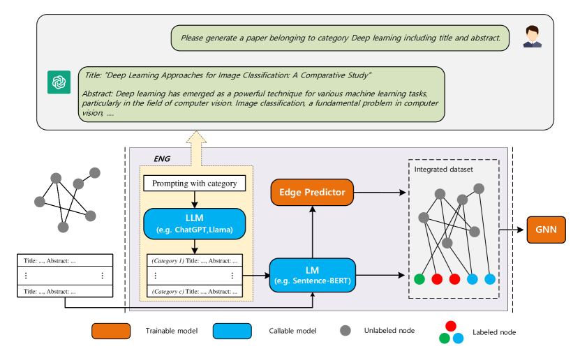
Figure 1. The overall paradigm of ENG.

2.1. Language Models on TAGs

When dealing with text-attributed graph data, GNNs often adopt the approach of processing text as a shallow non-contextual representation. However, language models have a better understanding of contextual relationships and can express textual content more effectively. Therefore, it becomes necessary to combine language models with graph neural networks to accomplish downstream tasks. For example, GIANT (Chien et al., 2021) extensively exploits the potential connections between graph structure and node attributes. It utilizes graph information to aid in feature extraction while fine-tuning language models. Graphformer (Yang et al., 2021) nests graph aggregation within Transformer blocks for text encoding, enabling a global understanding of the semantic meaning of each node. Further, GLEM (Zhao et al., 2022) trains graph neural networks and language models separately within a variational Expectation-Maximization framework, treating them as a process of knowledge distillation that mutually reinforces each other. With the emergence of LLMs, we can leverage more extensive knowledge and information. TAPE (He et al., 2023) utilizes LLMs to predict the ranked classification list of each node and outputs the corresponding explanations. Additionally, KEA (Chen et al., 2023) describes knowledge entities within the original text of each node to complement the textual content of the nodes. Although these methods have achieved some success, they often come with high computational or invocation costs and may not effectively address the challenges posed by few-shot scenarios with insufficient supervision signals.

2.2. Few-shot learning on Graphs

In the case of real-world graphs, acquiring labels is a resource-intensive task, making it a formidable challenge in few-shot scenarios. Some methods adopt the paradigm of meta-learning to handle few-shot problems on graphs (Wang et al., 2022a; Lan et al., 2020; Liu et al., 2021; Huang and Zitnik, 2020; Liu et al., 2022). In this paper, we focus on the semi-supervised setting, where each category has a few labeled samples. Self-supervised learning methods on graphs learn node representations through a pre-training task and fine-tuning for classification results using a few labeled nodes (Wan et al., 2021a; Zhu et al., 2020; Veličković et al., 2018; Hafidi et al., 2020; Wang et al., 2017). For example, GRACE (Zhu et al., 2020) and GraphCL (Hafidi et al., 2020) construct different views through data augmentation on graphs to bring positive samples closer and push negative samples further apart for learning node representations. Additionally, DGI (Veličković et al., 2018) stands as the pioneering method to introduce contrast between node-level embeddings and graph-level embeddings. This innovation empowers graph encoders to capture both local and global semantic information. MVGRL (Hassani and Khasahmadi, 2020) leverages first-order neighbor subgraphs and graph diffusion to generate contrastive views. However, when labeled data is extremely scarce leading to insufficient supervision signals, the model’s performance suffers. Several semi-supervised methods have been proposed to enhance model performance using limited labeled information. M3S (Sun et al., 2020) combines self-training and deep clustering to expand the training set by predicting high-confidence pseudo-labels. CGPN (Wan et al., 2021b) establishes a variational inference framework for Graph Poisson Network (GPN) and GNN models, and integrates contrastive learning to propagate limited label information over the entire graph. Meta-PN (Ding et al., 2022) generates high-quality pseudo-labels through meta-learning strategies to effectively enhance sparse label data. These methods leverage the information of the raw dataset to establish high-confidence pseudo-labels. The advent of LLMs provides us with a novel approach to address few-shot problem. We can harness these LLMs to unearth domain knowledge and generate extra supervision signals.

3. PRELIMINARY

[Text-Attributed Graphs]  A Text-Attributed Graph (TAG) is defined as $\mathcal{G}_{S}=(\mathcal{V},\mathcal{E},\mathcal{S}^{\mathcal{V}})$, where $\mathcal{V}$ represents a set of nodes and $\mathcal{E}\subseteq\mathcal{V}\times\mathcal{V}$ represents a set of edges. Each node $v_{i}\in\mathcal{V}$ is associated with a sequential text $s_{i}\in\mathcal{S}^{\mathcal{V}}$ and the corresponding label $y_{i}$. Each label has a real label text $c$ (e.g., ‘Machine Learning’ or ‘Databases’) from the set of all label texts $\mathcal{C}$. The corresponding adjacency matrix of the graph $\mathcal{G}_{S}$ is denoted by $A$. For simplicity, we set $A_{ij}$ = 1 if $e(v_{i},v_{j})\in\mathcal{E}$ ; 0, otherwise.

[Few-shot Node Classification]  In this paper, we focus on zero- and few-shot node classification, which is one of the most challenging and cutting-edge problems in the field of graph learning. Unlike the few-shot problem in the meta-learning paradigm, in our setting, each class has $K$ labeled samples. Given the labeled $K\times|\mathcal{C}|$ samples, our goal is to predict unlabeled samples in the test set, referred to as $K$-shot classification. Specifically, zero-shot classification means that there is no labeled sample.

[Graph Neural Network Architecture]   GNNs use input graph structure as the computation graph, aggregating information from a node’s neighbors, then updating the representation of each node. Formally, suppose $h^{(l)}_{v_{i}}$ is the representation of node $v_{i}$ at the $l$-th GNN layer, the updating procedure is:

(1) $$h^{(l)}_{v_{i}}=\underset{\forall v_{j}\in\mathcal{N}(v_{i}),\forall e\in\mathcal{E}(v_{i},v_{j})}{\text{Aggregate}}\left(\{\text{Propogate}(h^{(l-1)}_{v_{i}};h^{(l-1)}_{v_{j}},e)\}\right)$$

where $\mathcal{N}(v_{i})$ denotes the set of neighbors of node $v_{i}$ and $\mathcal{E}(v_{i},v_{j})$ denotes the set of edges connected from node $v_{j}$ to node $v_{i}$. Aggregate$(\cdot)$ and Propagate$(\cdot)$ are the two functions in GNNs. Propagate$(\cdot)$ represents the propagation of node information. It uses the target node’s representation $h^{(l-1)}_{v_{i}}$ and the edge $e$ between the two nodes as query, and propagates the information $h^{(l-1)}_{v_{j}}$ of the source node to the target node $v_{i}$. Aggregate$(\cdot)$ is a differentiable function (e.g., sum, mean, etc.) that aggregates the representations of a node’s neighbors.

4. method

This section introduces details of our proposed paradigm ENG. The general model diagram is shown in Figure 1. We guide LLM through prompt statements to generate some samples with labels and input these generated samples into LM together with the text in the raw dataset to obtain node representations. Subsequently, we perform supervised learning using the raw graph. We utilize the existing edges as supervision signals and input node embeddings to train the edge predictor. After training, we can utilize the embeddings to predict edges between nodes in the raw dataset and generated nodes. The newly generated nodes, along with their structural information, can be integrated into the original dataset. Finally, we can train the entire dataset using any GNNs and obtain results for node classification.

4.1. Sample Generation from LLM

When dealing with node classification tasks of a TAG in few-shot scenarios, we lack sufficient supervision signals to make accurate predictions. To address this, we can leverage the textual information within the set of label texts $\mathcal{C}$ to explore the semantics embedded in LLMs and generate $M$ relevant sample instances for each label. We generate a total of $M\times|\mathcal{C}|$ samples, $M\times|\mathcal{C}|\ll|\mathcal{V}|$, which is less costly compared to node-level augmentation. Specifically, we denote $c$ as one of the label texts. $\text{Prompt}(c)$ denotes the prompt statement containing the label text $c$. We feed it into LLM and then get the generated text $s_{g}$:

(2) $$s_{g}=\text{LLM}(\text{Prompt}(c)),\quad c\in\mathcal{C}$$

The text generated by LLM is based on the knowledge learned from the training corpora. It contains both samples that actually exist in the real world and pseudo-samples that the model creates internally by permutating the knowledge. Even though those pseudo-samples do not exist in reality, we can still trust them because our goal is to capture domain knowledge associated with the label. For instance, when performing interest classification of users in a social network, for the label “sports”, we can generate user profiles of individuals who are interested in basketball or soccer. Although these users do not actually exist, we can still uncover domain-specific information and capture the information that basketball and soccer related to the “sports” category.

4.2. Node representation initialization with LM

After generating new samples, we treat each of them as a new node $g_{i}$ on the TAG. Inspired by (Chen et al., 2023), deep sentence embeddings with GNNs have emerged as a powerful baseline compared to non-contextualized shallow embeddings. Moreover, sentence embedding models offer a lightweight approach to get representations without fine-tuning. Therefore, we adopt sentence embedding models to extract information from the text such as Sentence-BERT (Reimers and Gurevych, 2019) and e5-large (Wang et al., 2022b).

(3) $$h_{v_{i}}=\text{LM}(s_{v_{i}}),\quad h_{g_{i}}=\text{LM}(s_{g_{i}}),$$

where $s_{v_{i}}$ and $s_{g_{i}}$ denote the text of the raw dataset samples and the newly generated sample, respectively. $h_{v_{i}}$ and $h_{g_{i}}$ denote the corresponding representations of these samples. We denote $H_{n}=H_{v}\cup H_{g}$ as the representation of all nodes.

Table 1. Node classification performance in few-shot scenarios of Cora w.r.t. the classification accuracy. We highlight the best results in bold.

Methods	0-shot	1-shot	2-shot	3-shot	4-shot	5-shot	10-shot
GCN(Pyg)	-	60.32(4.12)	64.86(5.83)	68.30(4.81)	71.94(1.85)	75.74(1.81)	78.16(2.57)
GCN(MiniLM)	-	64.26(6.22)	69.28(5.56)	74.02(4.70)	75.64(2.93)	78.30(1.15)	80.24(1.58)
GAT(Pyg)	-	51.76(4.97)	55.90(4.61)	61.16(5.32)	67.74(2.14)	71.26(3.06)	75.38(3.26)
GAT(MiniLM)	-	60.02(6.24)	67.58(4.18)	72.14(5.46)	74.24(2.37)	76.90(1.61)	79.16(1.20)
DGI	-	62.06(7.40)	71.26(6.02)	72.96(2.88)	76.88(3.50)	78.42(2.11)	79.92(1.25)
MVGRL	-	61.94(10.64)	67.48(4.55)	67.68(1.83)	74.66(1.96)	76.98(3.27)	79.16(1.97)
GRACE	-	67.00(9.17)	68.78(3.98)	73.20(5.87)	75.36(2.33)	77.68(2.34)	80.12(1.03)
Meta-PN	-	59.20(10.99)	68.92(4.74)	75.30(1.80)	76.50(2.63)	77.10(3.37)	80.12(1.15)
CGPN	-	67.94(4.09)	73.46(2.78)	75.76(0.91)	75.70(1.80)	77.46(2.63)	77.80(0.61)
ENG+GCN	74.46(1.60)	76.48(0.90)	76.08(2.75)	76.26(2.88)	76.94(2.07)	79.06(0.75)	80.40(1.01)
ENG+GAT	74.14(1.22)	75.90(1.86)	75.44(2.38)	76.34(2.63)	76.40(1.51)	78.14(1.25)	79.60(1.16)
ENG+GCN w/o A	70.44(1.72)	75.12(1.60)	75.24(1.88)	76.04(3.21)	76.86(1.58)	79.28(1.20)	80.94(1.55)
ENG+GAT w/o A	74.08(1.49)	74.38(2.03)	75.00(4.36)	74.82(3.77)	75.98(3.42)	77.20(3.36)	78.82(2.57)
(improv.)	-	(+12.57%)	(+3.57%)	(+0.77%)	(+0.08%)	(+1.10%)	(+1.02%)

4.3. Edge Predictor

Next, we insert new nodes into the raw graph to establish connections between newly generated nodes $g_{i}$ and the raw nodes $v_{j}$. Edges play a role in message passing in the paradigm of GNNs, and new nodes with labels need to propagate supervision signals to other nodes without labels. We aim to ensure that unlabeled nodes receive as much relevant information from similar samples as possible to assist downstream classification tasks.

We consider this problem from two perspectives. First, we perform a coarse screening of potential edges between new nodes and raw nodes. To achieve this, we filter irrelevant edges by the cosine similarity of the representations in the latent space.

(4) $$e(h_{g_{i}},h_{v_{j}})\in\mathcal{E}_{P},\quad\text{if}\>\text{sim}(h_{g_{i}},h_{v_{j}})=h_{g_{i}}h_{v_{j}}^{T}>\delta$$

where $\delta$ as a hyper-parameter represents the similarity threshold. We add edges that have larger similarity weights than $\delta$ to the edge prediction set $\mathcal{E}_{P}$.

However, relying solely on node similarity to determine edge existence is too simple. It is also expected the newly added edges share high similarity with raw edges in the graph. To achieve this goal, we use the edges in the raw graph as supervision signals and construct an edge predictor for the link prediction task. Specifically, we create a binary classification task where the training set is constructed from the raw graph, and the test set is the edge prediction set $\mathcal{E}_{P}$. We take raw edges in the graph as positive samples while randomly sampling an equal number of non-existent edges as negative samples:

(5) $$y_{e}(h_{v_{i}},h_{v_{j}})=\left\{\begin{aligned} &\>1\quad\text{if }e(h_{v_{i}},h_{v_{j}})\in\mathcal{E}\\ &\>0\quad\text{if }e(h_{v_{i}},h_{v_{j}})\notin\mathcal{E}\\ \end{aligned}\right.$$

Then, we concatenate the representations of two-end nodes in each edge and feed them into a multi-layer perceptron (MLP) to obtain the probability of edge existence $\hat{y}_{e}$.

(6) $$\hat{y}_{e}(h_{v_{i}},h_{v_{j}})=\text{MLP}(h_{v_{i}}||h_{v_{j}})$$

We can formulate our cross-entropy loss function as:

(7) $$\mathcal{L}_{\text{CE}}(y_{e},\hat{y}_{e})=-[y_{e}\log(\hat{y}_{e})+(1-y_{e})\log(1-\hat{y}_{e})]$$

After training the edge predictor, we input the node pairs from the test set into the model to obtain the edge probabilities for the node pairs in the test set. We then select the top-$k$ edges with the highest probabilities and add them to the raw graph. This integrates the newly added nodes with the raw graph.

4.4. ENG

Finally, we derive the new adjacency matrix $A_{n}$ as well as the representations of nodes $H_{n}$, which are further fed into any GNNs along with the set of labeled nodes $\mathcal{Y}_{L}$ (a total of $(K+M)*|\mathcal{C}|$ samples) to output the classification results $Y_{n}$:

(8) $$Y_{n}=\text{GNN}(A_{n},H_{n},\mathcal{Y}_{L}).$$

The proposed paradigm ENG utilizes LLMs to mine semantic information of labels in few-shot scenarios, enabling sample generation and the establishment of supervision signals. Subsequently, we employ a simple model Edge Predictor to obtain additional structural information through training. Our proposed approach is lightweight, which allows us to facilitate node classification in few-shot scenarios by simply adding labeled nodes and edges without altering the raw dataset.

5. Experiment

5.1. Datasets

To evaluate the performance of ENG, we employ three citation network datasets: Cora (McCallum et al., 2000), Pubmed (Sen et al., 2008), and ogbn-arxiv (Hu et al., 2020). These datasets are citation networks that are widely used for node classification. In these datasets, each node represents a publication and the edges between nodes represent citations between the publications. In Cora, the papers belong to seven different classes within the field of computer science. These classes include Case-Based, Genetic Algorithms, Neural Networks, Probabilistic Methods, Reinforcement Learning, Rule Learning, and Theory. The medical literature in Pubmed is divided into three classes: Diabetes Mellitus, Experimental, Diabetes Mellitus Type 1 and Diabetes Mellitus Type 2. As for ogbn-arxiv , it is a large-scale dataset of 40 classes that encompasses papers from various disciplines, including computer science, mathematics, social sciences, and more.

Table 2. Node classification performance in few-shot scenarios of Pubmed w.r.t. the classification accuracy. We highlight the best results in bold.

Methods	0-shot	1-shot	2-shot	3-shot	4-shot	5-shot	10-shot
GCN(Pyg)	-	60.52(3.15)	63.16(2.45)	63.22(4.59)	65.58(3.58)	68.64(3.15)	75.26(2.48)
GCN(MiniLM)	-	63.02(3.71)	64.74(4.00)	65.82(2.24)	68.40(4.16)	70.06(4.33)	77.72(1.56)
GAT(Pyg)	-	59.72(4.14)	63.48(3.15)	63.76(2.87)	65.88(3.80)	66.92(3.84)	74.64(3.55)
GAT(MiniLM)	-	61.82(4.21)	63.22(5.70)	65.38(2.30)	66.56(2.96)	69.22(1.47)	76.02(1.86)
DGI	-	64.88(7.84)	64.70(9.13)	69.88(3.39)	70.98(3.72)	73.76(3.96)	77.96(0.95)
MVGRL	-	61.78(9.22)	64.7(10.64)	65.42(8.10)	69.36(1.08)	69.58(3.08)	75.16(4.41)
GRACE	-	63.80(1.93)	67.70(6.22)	68.74(6.06)	69.60(5.67)	71.46(7.00)	76.86(3.18)
Meta-PN	-	57.52(3.85)	59.56(6.16)	66.60(7.24)	69.52(9.38)	69.66(6.55)	74.28(4.84)
CGPN	-	59.03(10.05)	56.90(9.95)	63.00(11.36)	65.03(4.37)	64.73(7.68)	64.70(3.72)
ENG+GCN	75.36(2.43)	75.06(2.56)	76.82(4.30)	76.70(3.46)	76.74(2.55)	78.50(2.56)	80.54(0.78)
ENG+GAT	74.66(1.04)	75.98(2.82)	76.50(1.85)	76.06(2.67)	76.00(3.15)	78.04(2.22)	78.66(1.07)
ENG+GCN w/o A	73.72(2.88)	74.82(2.45)	75.56(3.17)	75.72(3.36)	76.06(2.68)	77.66(2.85)	79.64(1.33)
ENG+GAT w/o A	74.08(1.49)	74.38(2.03)	75.00(4.36)	74.82(3.77)	75.98(3.42)	77.20(3.36)	78.82(2.57)
(improv.)	-	(+15.70%)	(+13.47%)	(+9.76%)	(+8.11%)	(+6.42%)	(+3.31%)

Table 3. Node classification performance in few-shot scenarios of ogbn-arxiv w.r.t. the classification accuracy. We highlight the best results in bold. OOM denotes the out-of-the-memory error.

Methods	0-shot	1-shot	2-shot	3-shot	4-shot	5-shot	10-shot
GCN(Pyg)	-	23.38(5.26)	32.98(9.12)	39.77(6.36)	46.23(3.62)	47.95(2.24)	52.27(1.86)
GCN(MiniLM)	-	31.42(3.89)	40.63(10.52)	45.62(7.02)	55.30(4.08)	53.44(2.01)	56.48(1.24)
GAT(Pyg)	-	22.83(4.48)	24.82(6.01)	29.70(3.03)	40.39(4.03)	40.17(3.47)	50.13(2.28)
GAT(MiniLM)	-	32.19(5.17)	41.43(8.28)	45.03(5.66)	53.92(2.35)	51.94(1.80)	54.39(1.22)
DGI	-	25.75(5.97)	32.93(6.30)	36.47(7.78)	40.71(2.42)	42.32(3.11)	45.79(1.27)
MVGRL	-	16.24(1.71)	17.82(2.26)	21.58(4.11)	23.42(1.79)	24.50(1.45)	31.26(1.17)
GRACE	-	29.91(1.73)	35.72(2.35)	38.24(3.62)	38.68(1.11)	37.72(2.11)	43.51(0.91)
Meta-PN	-	23.38(6.10)	27.32(2.67)	31.47(0.73)	30.53(6.62)	34.67(3.68)	39.28(4.20)
CGPN	-	OOM	OOM	OOM	OOM	OOM	OOM
ENG+GCN	54.60(1.27)	56.83(1.82)	58.32(1.01)	58.70(1.54)	60.58(0.74)	60.83(0.88)	61.11(1.70)
ENG+GAT	54.35(1.97)	56.29(2.65)	56.76(1.71)	58.04(1.81)	60.03(1.45)	59.95(1.59)	61.40(1.06)
ENG+GCN w/o A	53.82(2.02)	55.89(1.30)	57.13(1.14)	58.68(0.41)	59.83(2.03)	58.87(1.40)	60.31(1.74)
ENG+GAT w/o A	54.13(0.71)	55.18(2.28)	56.50(1.75)	57.85(1.77)	59.70(1.72)	57.84(2.56)	59.89(0.91)
(improv.)	-	(+76.55%)	(+40.77%)	(+28.67%)	(+9.55%)	(+13.83%)	(+8.71%)

5.2. Baselines

We also compare ENG with 7 other SOTA baselines, which can be categorized into three groups:

$\bullet$ [Classical base models]: GCN (Kipf and Welling, 2016) and GAT (Veličković et al., 2017) are common benchmark models in graph learning for node-level representation learning based on graph convolution and attention mechanisms, respectively.

$\bullet$ [Graph self-supervised models]: DGI (Veličković et al., 2018), MVGRL (Hassani and Khasahmadi, 2020), and GRACE (Zhu et al., 2020) are prominent benchmark approaches in graph neural networks for self-supervised learning tasks. DGI focuses on maximizing the alignment between node representations and global summary vectors. Both MVGRL and GRACE use data augmentation to generate different views for contrastive learning, the former adopts graph diffusion and subgraph sampling techniques, while the latter employs edge dropping and node feature masking.

$\bullet$ [Graph models in few-shot scenarios]: CGPN (Wan et al., 2021b) is inspired by Poisson Learning and propagates limited labels to the entire graph by contrastive learning between two networks. Meta-PN (Ding et al., 2022) employs a meta-learning strategy to generate high-quality pseudo-labels, effectively enhancing scarce labeled data.

When running GCN and GAT, we execute the features built into PyG (Fey and Lenssen, 2019) and the sentence embeddings obtained from LM each once. For other methods, we follow the settings described in their original paper.

5.3. Experimental Settings

In ENG, we adopt Sentence-BERT (Reimers and Gurevych, 2019) (MiniLM) as LM to obtain sentence embeddings. As for LLM, we use ChatGPT (Brown et al., 2020) (i.e., “gpt-3.5-turbo”) and a basic form of prompt ENG-P1 in Table 4 to generate samples. We set the number of generated samples per class $M$ to be 10 across all datasets. The similarity threshold $\delta$ is chosen from 0.1 to 0.8 with step size 0.1. Regarding the selection of top-$k$ node pairs in the set of edge prediction set $\mathcal{E}_{P}$, we fine-tune the values $k$ to be $1\times$, $5\times$, $10\times$, $30\times$, $50\times$, $70\times$, $100\times$, and $200\times$ of the number of generated samples $M|\mathcal{C}|$. We use the integrated new graph as input data and conduct experiments on different shot scenarios using two backbone models, GCN and GAT, to verify the effectiveness of our proposed paradigm. The notation “w/o A” indicates the absence of an edge predictor module, meaning that the generated labeled samples are treated as isolated points during model training. For fair comparison, we report the average results on the test set with standard deviations of 5 runs for all experiments. We run all the experiments on a server with 32G memory and a single Tesla V100 GPU.

Due to the space limitation, we move the experimental setup (Sec. A.2), hyperparameter analysis (Sec. A.3), and instances of generating samples using LLMs (Sec. A.4) to Appendix.

5.4. Performance Comparison

We perform zero- and few-shot node classification on TAGs. We construct a $K$-shot training set, where each class includes $K$ samples, with $K$ values chosen from the set $\{0,1,2,3,4,5,10\}$. For Cora and PubMed, we randomly sample $K\times|\mathcal{C}|$ nodes from all the nodes as the training set. From the remaining nodes, we randomly select 500 nodes as the validation set and 1000 nodes as the test set. For ogbn-arxiv, we follow its original partitioning, but we reduce the size of the training set to the $K$-shot setting as specified. The results are reported in Table 1, 2 and 3. From the table, we have the following observations:

(1) In all cases, ENG has demonstrated exceptional performance, particularly in low-shot scenarios. For example, on the ogbn-arxiv dataset, the accuracy of ENG  achieves 56.83% in the 1-shot setting, while the runner-up method achieves only 31.42%. We have achieved a remarkable improvement of 76% over the baseline model. Furthermore, our proposed paradigm ENG has significant enhancements on both GCN and GAT backbone models. This all indicates that the supervision signals provided by the generated samples are particularly helpful to the model.

(2) ENG achieves impressive performance in zero-shot scenarios by generated samples that outperforms even other methods in low-shot scenarios. On Pubmed, the accuracy of our model in the 0-shot scenario exceeds other models across different shot settings, except for the 10-shot scenario. This trend is also observed in the ogbn-arxiv dataset. ENG provides a method that can be trained by GNNs in zero-shot scenarios.

(3) In few-shot scenarios, the structural information between the generated nodes and the nodes in the raw dataset has demonstrated positive effects. It plays a crucial role in improving model performance. This is because the structure promotes supervision signals to propagate, allowing unlabeled nodes to be susceptible to labeled nodes, which improves the model.

In conclusion, the strong performance of ENG highlights the effectiveness of leveraging generated samples to enhance the model’s learning capabilities, especially when labeled data is extremely scarce.

Table 4. Prompt statements for LLMs to generate samples.

Prompt 1:

Please generate a paper belonging to category [class name], including title and abstract.

Prompt 2:

We want to generate a few nodes from graph-structured data where the nodes represent individual research papers and the edges represent citation relationships among the papers.

Please generate a paper belonging to category [class name], including title and abstract.

Prompt 3:

Here are two papers belonging to category [class name], $[$paper1 title and abstract$]$, $[$paper2 title and abstract$]$. Please generate another paper belonging to category [class name], including title and abstract.

Prompt 4:

We have some research paper topics, namely Case Based, Genetic Algorithms, Neural Networks, Probabilistic Methods, Reinforcement Learning, Rule Learning and Theory.

Please generate a title and abstract for each of these topics.

Prompt 5:

Please generate 10 papers belonging to category [class name], including title and abstract.

Prompt 6:

User: Please generate a paper belonging to category [class name], including title and abstract.

LLM:  Title:… Abstract:…

User:  The title of the paper you generated previously is [Generated paper1 title]. Please generate a paper belonging to category [class name], including title and abstract, which is different from the previous one you generated.

LLM:  Title:… Abstract:…

User:  The title of the paper you generated previously is [Generated paper1 title],[Generated paper2 title]. Please generate a paper belonging to category [class name], including title and abstract, which is different from the previous one you generated.

…

5.5. Case Study of Generated Samples

In this section, we analyze the impact of prompt statements, the quantity of generated samples and LLMs’ stochasticity during sample generation on the performance of the model in the Cora dataset. The experiments conducted in this section are run only once and do not involve edge prediction between the generated nodes and the nodes in the raw dataset.

Prompt statements.  We validate the impact of different prompt statements on the quality of generated samples. We design six different prompt statements and ensure an equal number of generated samples (i.e., 70 samples) for each case. These statements indicate as follows: (1) ENG-P1 is a basic form of prompt that directly generates samples related to the category. (2) Building upon ENG-P1, ENG-P2 includes a description of the text generation task, introducing the roles of nodes and edges in the graph data. (3) ENG-P3 takes the samples from the training set as exemplars for LLM and generates samples based on them. (4) ENG-P4 provides all the labels for LLM to generate $|\mathcal{C}|$ samples in one go. (5) Compared to ENG-P4 based on all categories, ENG-P5 generates $M$ samples based on a specific category. (6) For ENG-P6, LLM generates different samples based on previously generated samples.

Table 5. Impact of different prompt statements on the model performance.

Prompt	0-shot	1-shot	2-shot	3-shot	5-shot	10-shot
ENG-P1	71.0	73.9	78.1	76.5	80.2	82.9
ENG-P2	67.4	74.8	76.2	77.1	79.1	81.9
ENG-P3	-	78.2	76.5	75.8	78.9	81.7
ENG-P4	73.7	77.4	80.1	78.7	81.6	84.0
ENG-P5	65.4	74.0	76.5	77.4	78.9	82.5
ENG-P6	64.9	72.9	77.9	77.4	79.8	81.8

In Table 4, we list specific examples of prompt statements. By comparing the experimental results in Table 5 and the differences among the raw texts of the generated samples, we find that:

(1) Compared to the basic form of prompt ENG-P1, ENG-P2 has an improvement in accuracy for 1-shot and 3-shot scenarios, indicating that the task description in the prompt enables LLM to better understand the task and generate more accurate samples related to the task. However, there is a decrease in accuracy in other scenarios, suggesting that the content of the task description may need further optimization.

(2) In ENG-P3, there is a significant improvement in accuracy for the 1-shot scenario, but a decrease in accuracy for subsequent shots. This might be because only one sample is provided as an exemplar in the 1-shot scenario, and the generated samples display a high degree of relevance to the raw dataset. However, as the number of exemplars provided to LLM increases, the generated samples may lack diversity. Therefore, when providing the number of exemplars in the prompt statement, a balance needs to be struck between the diversity of the generated samples and their relevance to the raw dataset.

(3) ENG-P4 shows a boost in each scenario, as providing all label information to LLM enables it to grasp the semantic information of all labels and explore the differences between them, thus generating more indistinguishable samples and enhancing model performance. However, such prompts also have limitations, as generating a large number of samples in one go may be limited by output text length, especially in scenarios with a large number of categories.

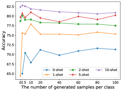
Figure 2. Impact of the quantity of generated samples on model performance

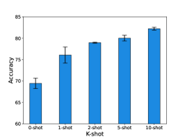
Figure 3. Impact of LLMs’ stochasticity on model performance

(4) ENG-P5 explores the characteristics and variations of each category to generate more diverse samples, while ENG-P6 aims to generate more distinctive samples. Compared to the samples generated from other prompt statements, these two methods generate richer samples in terms of sentence structure and content. However, such samples may lack connection with the raw dataset or label text, resulting in no gains in accuracy.

In summary, there are two main factors that influence the quality of generated samples by prompt statements. The first factor is the label information, as LLM can generate more distinctive samples by uncovering the differences between labels. The second factor is the balance between sample diversity and relevance to the raw dataset. Samples that are related to the raw dataset can narrow the gap between the generated nodes and the original nodes, while more diverse samples can make the label space more distinct. However, there is often a trade-off between these two factors, so maintaining a balance in the prompt statement can maximize the performance of the model.

The quantity of generated samples. In this case, we use the same prompt statement ENG-P1 to generate $100\times 7$ samples $(M\times|\mathcal{C}|)$, and conduct experiments under different shot settings. Subsequently, we vary the number of samples generated for each class and plot the experimental results in Figure 2. We note that as the number of generated samples increases, the accuracy shows an initial increase followed by a decrease, and eventually stabilizes. This phenomenon can be explained by the increased diversity of the generated samples, which allows the model to obtain richer supervised signals and improve performance. With an increasing number of generated samples, the additional samples gradually diminish their contribution to the model’s performance, and thus the results are not significantly improved.

LLMs’ stochasticity. We also repeat the same prompt statement ENG-P1 five times to generate different sample contents, where the number of generated samples $M$ is 10, i.e., a total of 350 ($5\times 10(M)\times 7(|\mathcal{C}|))$ samples. We ensure that the generated samples are not identical to each other. From Figure 3, we observe that although there are variations among the generated samples, the overall quality is quite good, exhibiting strong generalization capabilities. We believe that the effectiveness of the generated samples by LLMs lies in their ability to capture semantic information relevant to the label text. This semantic information is reliable and has a positive impact on classification results.

6. conclusion

In this study, we proposed a lightweight paradigm called ENG  to address the node classification problem in few-shot scenarios. Specifically, we leveraged the powerful generation capabilities of LLMs to explore the semantic information of labels and generate samples. We then trained an edge predictor to incorporate these generated samples into the raw dataset, thereby providing supervision signals to the model. The impressive experimental results strongly demonstrated the effectiveness of ENG.

In our future work, we will continue to delve into how to utilize LLMs to generate supervision signals and improve model performance. Firstly, for other weakly supervised scenarios, including label imbalance and label noise, our goal is to leverage LLMs to supplement samples from imbalanced classes and correct mislabeled samples. Secondly, in the case of high labeling rates, we will investigate how to generate more diverse samples using known labeled samples to enrich the diversity of the supervision signals and enhance the generalization ability of the model. Furthermore, existing approaches utilize LLMs to augment the dataset at the node level and class level. However, topological information is also crucial for graphs. Since LLMs may not fully grasp the complexity of structural information, generating topology-based supervision signals using LLMs remains a challenging problem. Overall, we will continue to explore the combination of LLMs with graph learning in various domains.

Appendix A Appendix

A.1. Dataset Description

The ogbn-arxiv dataset originates from the well-known OGB benchmark (Hu et al., 2020). The categories include 40 classes such as “Numerical Analysis”, “Multimedia”, “Logic in Computer Science”, and more. Specific information can be found in https://ogb.stanford.edu/docs/nodeprop/ . Table 6 provides statistics of three datasets.

Table 6. Statistics of datasets

Dataset	Nodes	Edges	Classes
Cora	2,708	5,429	7
Pubmed	19,717	44,338	3
ogbn-arxiv	169,343	1,166,243	40

A.2. Experiment Setups

For the GCN, GAT, and ENG-based methods, we use the same range of hyperparameters. For the other methods, we follow the hyperparameter setting in their reporsitory ^{, , , ,} . The search space is proivded as:

1. Hidden dimension:$\{$16, 32, 64, 128, 256$\}$

2. Dropout: $\{$0.0, 0.2, 0.5, 0.8$\}$

3. Learning rate: $\{$1e-2, 5e-2, 5e-3, 1e-3$\}$

4. Weight Decay: $\{$5e-4, 5e-5, 0$\}$

A.3. Hyperparameter Analysis

We further perform a sensitivity analysis on the hyperparameters of our paradigm. We study two main hyper-parameters in ENG: the similarity threshold $\delta$ in Eq. 4 and the number of edges connected between the generated nodes and the raw graph nodes $k$. In our experiments, we vary one parameter each time with others fixed. From the Figure 4, we see that:

(1) In the case of the threshold $\delta$, we fix the number of edges on the Pubmed dataset by choosing 70 times the number of generated samples, i.e., 2100. We observe that as the threshold increases, the accuracy initially increases and then decreases. This is because when the threshold is too low, the structure includes many noisy edges, resulting in connecting irrelevant nodes. These erroneous connections propagate incorrect information during message passing, thereby reducing the accuracy. On the other hand, when the threshold is too high, the number of node pairs available for edge prediction in the edge set decreases. The newly connected nodes are already easily distinguishable samples, providing limited assistance for hard samples. Therefore, a high threshold restricts the benefits of structural information, leading to a decrease in accuracy.

(2) For the number of connected edges $k$, there is a consistent trend in most scenarios. When the number of edges is too few, the newly generated nodes may not have enough connections to effectively propagate the supervision signals. This means that the information propagation between nodes is limited, and the model may struggle to accurately learn the relationships and features among the nodes, thus impacting the model’s performance. Further, when the number of edges is too high, there may be an issue of over-smoothing. Having an excessive number of edges can lead to excessive mixing of information between node representations, resulting in similar node representations. This can confuse the model during prediction, making it difficult to accurately differentiate between different nodes and decreasing the accuracy. In the 10-shot scenario with more supervision signals, the discrepancy between node representations can also be recognized in the case of more edges, resulting in better model performance.

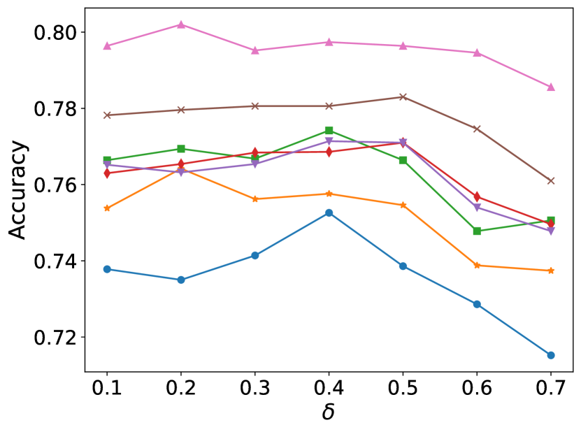
(a)

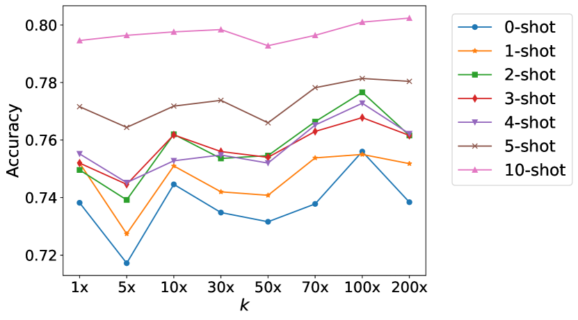
(b)

Figure 4. Hyper-parameter sensitivity analysis on the Pubmed dataset. $\delta$ is the similarity threshold and $k$ is the number of connected edges.

Table 7. Title of the samples generated with the label “Graph”

ID	Title
1	Graph-Based Recommendation Systems: An Overview and Evaluation of Algorithms.
2	A Comparative Study of Graph-Based Approaches for Community Detection in Social Networks.
3	Graph-based Analysis of Social Networks: Uncovering Community Structure and Influence Dynamics.
4	Analysis of Graph Coloring Algorithms and Their Application in Network Optimization.
5	Graph Analysis for Social Network Modeling and Information Diffusion.
6	Analyzing the Effectiveness of Graph-Based Algorithms for Social Network Analysis.
7	The Impact of Graph Theory in Network Analysis: A Comprehensive Review.
8	Graph Neural Networks: A Survey and Analysis.
9	The Impact of Graph Visualization Techniques on Decision-Making: A Comparative Analysis.
10	Graph Theory: Applications and Algorithms for Network Analysis.

Table 8. An illustrative example of calling LLMs on ogbn-arxiv

User:

Please generate a paper belonging to category Artificial Intelligence, including title and abstract.

LLM:

Title: A Comprehensive Survey of Artificial Intelligence Techniques for Autonomous Vehicle Navigation.

Abstract: With the rapid advancements in computer vision and machine learning, artificial intelligence (AI) has emerged as a crucial component for the development of autonomous vehicles. The integration of AI techniques enables vehicles to perceive their environment, make intelligent decisions, and navigate safely through complex scenarios. This paper provides a comprehensive survey of various AI techniques employed in autonomous vehicle navigation, including perception, planning, and control. We analyze state-of-the-art approaches, discuss their strengths and limitations, and highlight ongoing research challenges in the field. Furthermore, we investigate the impact of AI advancements on improving navigation accuracy, robustness, and scalability, and outline potential future directions for the continued development of autonomous driving technology.

A.4. Instances of Generating Samples using LLMs

Table 7 showcases ten instance titles generated using the basic prompt statement ENG-P1 for the “Graph” label, based on the ogbn-arxiv dataset. We have omitted the abstract of these papers. From these titles, it is evident that LLM can capture a multitude of knowledge related to the ”Graph” domain, such as recommendation systems, community detection, graph theory, and social networks. Although these papers do not exist in the real world, they can contain valuable knowledge about the graph domain. Hence, we can utilize these generated samples as supervision signals to enhance the model’s performance. In Table 8, we present a specific example of invoking LLM to generate samples on the ogbn-arxiv dataset. We can observe that the generated text is grammatically correct, logically coherent, and introduces another domain related to artificial intelligence, namely autonomous vehicle. Additionally, the text mentions various keywords associated with artificial intelligence, such as computer vision, machine learning, accuracy, and robustness. This demonstrates the ability of LLM to mine the domain knowledge of artificial intelligence. Furthermore, the generated text does not require any additional processing and can be directly input into LM to obtain embeddings.

References

- (1)
- Benamira et al. (2019) Adrien Benamira, Benjamin Devillers, Etienne Lesot, Ayush K Ray, Manal Saadi, and Fragkiskos D Malliaros. 2019. Semi-supervised learning and graph neural networks for fake news detection. In Proceedings of the 2019 IEEE/ACM International Conference on Advances in Social Networks Analysis and Mining. 568–569.
- Brown et al. (2020) Tom Brown, Benjamin Mann, Nick Ryder, Melanie Subbiah, Jared D Kaplan, Prafulla Dhariwal, Arvind Neelakantan, Pranav Shyam, Girish Sastry, Amanda Askell, et al. 2020. Language models are few-shot learners. Advances in neural information processing systems 33 (2020), 1877–1901.
- Chen et al. (2023) Zhikai Chen, Haitao Mao, Hang Li, Wei Jin, Hongzhi Wen, Xiaochi Wei, Shuaiqiang Wang, Dawei Yin, Wenqi Fan, Hui Liu, et al. 2023. Exploring the potential of large language models (llms) in learning on graphs. arXiv preprint arXiv:2307.03393 (2023).
- Chien et al. (2021) Eli Chien, Wei-Cheng Chang, Cho-Jui Hsieh, Hsiang-Fu Yu, Jiong Zhang, Olgica Milenkovic, and Inderjit S Dhillon. 2021. Node feature extraction by self-supervised multi-scale neighborhood prediction. arXiv preprint arXiv:2111.00064 (2021).
- Devlin et al. (2018) Jacob Devlin, Ming-Wei Chang, Kenton Lee, and Kristina Toutanova. 2018. Bert: Pre-training of deep bidirectional transformers for language understanding. arXiv preprint arXiv:1810.04805 (2018).
- Ding et al. (2022) Kaize Ding, Jianling Wang, James Caverlee, and Huan Liu. 2022. Meta propagation networks for graph few-shot semi-supervised learning. In Proceedings of the AAAI Conference on Artificial Intelligence, Vol. 36. 6524–6531.
- Du et al. (2021) Zhengxiao Du, Yujie Qian, Xiao Liu, Ming Ding, Jiezhong Qiu, Zhilin Yang, and Jie Tang. 2021. Glm: General language model pretraining with autoregressive blank infilling. arXiv preprint arXiv:2103.10360 (2021).
- Fan et al. (2023) Wenqi Fan, Zihuai Zhao, Jiatong Li, Yunqing Liu, Xiaowei Mei, Yiqi Wang, Jiliang Tang, and Qing Li. 2023. Recommender systems in the era of large language models (llms). arXiv preprint arXiv:2307.02046 (2023).
- Fey and Lenssen (2019) Matthias Fey and Jan Eric Lenssen. 2019. Fast graph representation learning with PyTorch Geometric. arXiv preprint arXiv:1903.02428 (2019).
- Hafidi et al. (2020) Hakim Hafidi, Mounir Ghogho, Philippe Ciblat, and Ananthram Swami. 2020. GraphCL: Contrastive Self-Supervised Learning of Graph Representations. arXiv:2007.08025 [cs.LG]
- Harris (1954) Zellig S Harris. 1954. Distributional structure. Word 10, 2-3 (1954), 146–162.
- Hassani and Khasahmadi (2020) Kaveh Hassani and Amir Hosein Khasahmadi. 2020. Contrastive multi-view representation learning on graphs. In International conference on machine learning. PMLR, 4116–4126.
- He et al. (2020) Pengcheng He, Xiaodong Liu, Jianfeng Gao, and Weizhu Chen. 2020. Deberta: Decoding-enhanced bert with disentangled attention. arXiv preprint arXiv:2006.03654 (2020).
- He et al. (2023) Xiaoxin He, Xavier Bresson, Thomas Laurent, and Bryan Hooi. 2023. Explanations as Features: LLM-Based Features for Text-Attributed Graphs. arXiv preprint arXiv:2305.19523 (2023).
- Hu et al. (2020) Weihua Hu, Matthias Fey, Marinka Zitnik, Yuxiao Dong, Hongyu Ren, Bowen Liu, Michele Catasta, and Jure Leskovec. 2020. Open graph benchmark: Datasets for machine learning on graphs. Advances in neural information processing systems 33 (2020), 22118–22133.
- Huang and Zitnik (2020) Kexin Huang and Marinka Zitnik. 2020. Graph meta learning via local subgraphs. Advances in neural information processing systems 33 (2020), 5862–5874.
- Kipf and Welling (2016) Thomas N Kipf and Max Welling. 2016. Semi-supervised classification with graph convolutional networks. arXiv preprint arXiv:1609.02907 (2016).
- Lan et al. (2020) Lin Lan, Pinghui Wang, Xuefeng Du, Kaikai Song, Jing Tao, and Xiaohong Guan. 2020. Node classification on graphs with few-shot novel labels via meta transformed network embedding. Advances in Neural Information Processing Systems 33 (2020), 16520–16531.
- Li et al. (2023) Jiatong Li, Yunqing Liu, Wenqi Fan, Xiao-Yong Wei, Hui Liu, Jiliang Tang, and Qing Li. 2023. Empowering Molecule Discovery for Molecule-Caption Translation with Large Language Models: A ChatGPT Perspective. arXiv preprint arXiv:2306.06615 (2023).
- Liu et al. (2022) Yonghao Liu, Mengyu Li, Ximing Li, Fausto Giunchiglia, Xiaoyue Feng, and Renchu Guan. 2022. Few-shot node classification on attributed networks with graph meta-learning. In Proceedings of the 45th international ACM SIGIR conference on research and development in information retrieval. 471–481.
- Liu et al. (2021) Zemin Liu, Yuan Fang, Chenghao Liu, and Steven CH Hoi. 2021. Relative and absolute location embedding for few-shot node classification on graph. In Proceedings of the AAAI conference on artificial intelligence, Vol. 35. 4267–4275.
- McCallum et al. (2000) Andrew Kachites McCallum, Kamal Nigam, Jason Rennie, and Kristie Seymore. 2000. Automating the construction of internet portals with machine learning. Information Retrieval 3 (2000), 127–163.
- Miaschi and Dell’Orletta (2020) Alessio Miaschi and Felice Dell’Orletta. 2020. Contextual and Non-Contextual Word Embeddings: an in-depth Linguistic Investigation. In Proceedings of the 5th Workshop on Representation Learning for NLP. Association for Computational Linguistics, Online, 110–119. https://doi.org/10.18653/v1/2020.repl4nlp-1.15
- Nguyen et al. (2020) Van-Hoang Nguyen, Kazunari Sugiyama, Preslav Nakov, and Min-Yen Kan. 2020. Fang: Leveraging social context for fake news detection using graph representation. In Proceedings of the 29th ACM international conference on information & knowledge management. 1165–1174.
- Ni et al. (2019) Jianmo Ni, Jiacheng Li, and Julian McAuley. 2019. Justifying Recommendations using Distantly-Labeled Reviews and Fine-Grained Aspects. In Proceedings of the 2019 Conference on Empirical Methods in Natural Language Processing and the 9th International Joint Conference on Natural Language Processing (EMNLP-IJCNLP). Association for Computational Linguistics, Hong Kong, China, 188–197. https://doi.org/10.18653/v1/D19-1018
- Reimers and Gurevych (2019) Nils Reimers and Iryna Gurevych. 2019. Sentence-bert: Sentence embeddings using siamese bert-networks. arXiv preprint arXiv:1908.10084 (2019).
- Salton and Buckley (1988) Gerard Salton and Christopher Buckley. 1988. Term-weighting approaches in automatic text retrieval. Information processing & management 24, 5 (1988), 513–523.
- Sen et al. (2008) Prithviraj Sen, Galileo Namata, Mustafa Bilgic, Lise Getoor, Brian Galligher, and Tina Eliassi-Rad. 2008. Collective classification in network data. AI magazine 29, 3 (2008), 93–93.
- Sun et al. (2020) Ke Sun, Zhouchen Lin, and Zhanxing Zhu. 2020. Multi-stage self-supervised learning for graph convolutional networks on graphs with few labeled nodes. In Proceedings of the AAAI conference on artificial intelligence, Vol. 34. 5892–5899.
- Touvron et al. (2023) Hugo Touvron, Thibaut Lavril, Gautier Izacard, Xavier Martinet, Marie-Anne Lachaux, Timothée Lacroix, Baptiste Rozière, Naman Goyal, Eric Hambro, Faisal Azhar, et al. 2023. Llama: Open and efficient foundation language models. arXiv preprint arXiv:2302.13971 (2023).
- Veličković et al. (2017) Petar Veličković, Guillem Cucurull, Arantxa Casanova, Adriana Romero, Pietro Lio, and Yoshua Bengio. 2017. Graph attention networks. arXiv preprint arXiv:1710.10903 (2017).
- Veličković et al. (2018) Petar Veličković, William Fedus, William L Hamilton, Pietro Liò, Yoshua Bengio, and R Devon Hjelm. 2018. Deep graph infomax. arXiv preprint arXiv:1809.10341 (2018).
- Wan et al. (2021a) Sheng Wan, Shirui Pan, Jian Yang, and Chen Gong. 2021a. Contrastive and generative graph convolutional networks for graph-based semi-supervised learning. In Proceedings of the AAAI conference on artificial intelligence, Vol. 35. 10049–10057.
- Wan et al. (2021b) Sheng Wan, Yibing Zhan, Liu Liu, Baosheng Yu, Shirui Pan, and Chen Gong. 2021b. Contrastive graph poisson networks: Semi-supervised learning with extremely limited labels. Advances in Neural Information Processing Systems 34 (2021), 6316–6327.
- Wang et al. (2017) Chun Wang, Shirui Pan, Guodong Long, Xingquan Zhu, and Jing Jiang. 2017. Mgae: Marginalized graph autoencoder for graph clustering. In Proceedings of the 2017 ACM on Conference on Information and Knowledge Management. 889–898.
- Wang et al. (2022b) Liang Wang, Nan Yang, Xiaolong Huang, Binxing Jiao, Linjun Yang, Daxin Jiang, Rangan Majumder, and Furu Wei. 2022b. Text embeddings by weakly-supervised contrastive pre-training. arXiv preprint arXiv:2212.03533 (2022).
- Wang et al. (2022a) Song Wang, Kaize Ding, Chuxu Zhang, Chen Chen, and Jundong Li. 2022a. Task-adaptive few-shot node classification. In Proceedings of the 28th ACM SIGKDD Conference on Knowledge Discovery and Data Mining. 1910–1919.
- Yang et al. (2021) Junhan Yang, Zheng Liu, Shitao Xiao, Chaozhuo Li, Defu Lian, Sanjay Agrawal, Amit Singh, Guangzhong Sun, and Xing Xie. 2021. GraphFormers: GNN-nested transformers for representation learning on textual graph. Advances in Neural Information Processing Systems 34 (2021), 28798–28810.
- Yao et al. (2019) Liang Yao, Chengsheng Mao, and Yuan Luo. 2019. Graph convolutional networks for text classification. In Proceedings of the AAAI conference on artificial intelligence, Vol. 33. 7370–7377.
- Zhao et al. (2022) Jianan Zhao, Meng Qu, Chaozhuo Li, Hao Yan, Qian Liu, Rui Li, Xing Xie, and Jian Tang. 2022. Learning on large-scale text-attributed graphs via variational inference. arXiv preprint arXiv:2210.14709 (2022).
- Zhu et al. (2021) Jason Zhu, Yanling Cui, Yuming Liu, Hao Sun, Xue Li, Markus Pelger, Tianqi Yang, Liangjie Zhang, Ruofei Zhang, and Huasha Zhao. 2021. Textgnn: Improving text encoder via graph neural network in sponsored search. In Proceedings of the Web Conference 2021. 2848–2857.
- Zhu et al. (2020) Yanqiao Zhu, Yichen Xu, Feng Yu, Qiang Liu, Shu Wu, and Liang Wang. 2020. Deep graph contrastive representation learning. arXiv preprint arXiv:2006.04131 (2020).