Abstract

To ensure privacy protection and alleviate computational burden, we propose a Poisson-subsampling based distributed estimation procedure for the Cox model with massive survival datasets from multi-centered, decentralized sources. The proposed estimator is computated based on optimal subsampling probabilities that we derived and enables transmission of subsample-based summary level statistics between different storage sites with only one round of communication. For inference, the asymptotic properties of the proposed estimator were rigorously established. An extensive simulation study demonstrated that the proposed approach is effective. The methodology was applied to analyze a large dataset from the U.S. airlines.

Keywords: Empirical process; Distributed learning; L-optimality criterion; Massive survival data.

1 Introduction

The ubiquity of vast data volumes and privacy preserving needs are becoming defining characteristics when analyzing massive survival data from multi-centered, decentralized sources. With limited computational resources, traditional statistical tools using centralized data are no longer feasible to address either challenge. For effective processing with big data, subsampling is a popular statistical technique that can significantly alleviate both computational and storage burdens. In recent years, literature on subsampling-based methods for survival analysis with massive data have been developed. For example, Yang et al. (2022) considered the optimal subsampling algorithms for parametric accelerate failure time models. Keret and Gorfine (2023) and Zhang et al. (2023) proposed optimal subsampling procedures for Cox regression in context of rare or non-rate events. Comprehensive reviews on general subsampling-based big data analysis can be found in Yao and Wang (2021) and Yu et al. (2023), which also collects subsampling-based regression with non-survival data (Wang et al., 2018; Wang et al., 2019; Wang and Zhang, 2022; Han et al., 2020; Wang and Ma, 2021). For privacy preservation with decentralized data, distributed learning has been gaining increasing popularity as a solution that utilizes sabsample-based summary level statistics only. Several recent works indiacte that distributed learning in combination with subsampling techniques can balance the needs for privacy protection and maximized utilization of informative samples (Zhang and Wang, 2021; Zuo et al., 2021; Yu et al., 2022). However, there is a paucity of research on analysis of large-scale for survival data that leverages the benefits of both subsampling and distributed learning.

In this paper, we propose an approach for Cox regression that integrates subsampling and distributed learning techniques. The main idea involves conducting Poisson subsampling on individual datasets separately, and subsequently, constructing a distributed subsample estimator using summary-level statistics from multiple datasets. Compared to prior efforts for the Cox model (Keret and Gorfine, 2023; Zhang et al., 2023), our method offers several key advantages: first, when the Poisson subsampling is employed in Cox regression on each individual dataset, there is no duplication in the subsamples, and hence avoids unnecessary efficiency loss as compared to exiting methods (Keret and Gorfine, 2023; Zhang et al., 2023). Second, our approach can effectively address the issue of “isolated data island” in big data by accommodating multiple datasets, rather than being restricted to single datasets alone. In addition, the proposed estimator enables privacy-preserving transmission of subsample-based summary level statistics between different storage sites with only one round of communication.

The remainder of this paper is organized as follows: In Section 2, we introduce notation and definitions associated with the Cox model. In Section 3, we establish the optimal subsampling probabilities based on the Poisson subsampling approach, and propose a distributed subsample estimator with rigorously derived asymptotic properties. In Section 4, we demonstrate the effectiveness of our approach through simulation studies and an illustrative example for real-world applications. Some concluding remarks are provided in Section 5, and detailed proofs are presented in the Appendix.

2 Model and Notation

Let $T$ denote the failure time, $C$ represent the censoring time, and $\mathbf{X}$ be a $p$-dimensional vector of covariates. Given $\mathbf{X}$, we assume that $T$ and $C$ are conditionally independent. The observed failure time is $Y=\min(T,C)$ with the failure indicator $\Delta=I(T\leq C)$, where $I(\cdot)$ represents the indicator function. The Cox’s proportional hazard regression model Cox (1972) assumes that the conditional hazard rate function of $T$ given $\mathbf{X}$ is

$$\lambda(t|\mathbf{X})=\lambda_{0}(t)\exp(\bm{\beta}^{\prime}\mathbf{X}),$$ (1)

where $\lambda_{0}(t)$ represents an unknown baseline hazard function, $\bm{\beta}=(\beta_{1},\cdots,\beta_{p})^{\prime}$ is a $p$-dimensional vector of regression parameters with its true value is constrained within a compact set $\Theta\subset\mathbb{R}^{p}$.

Assume that we observe $K$ large survival datasets denoted as $\mathcal{D}_{n_{k}}=\{(\mathbf{X}_{ik},\Delta_{ik},Y_{ik}),i=1,\cdots,n_{k}\}$, where $n_{k}$ represents the sample size of $\mathcal{D}_{n_{k}}$ for $k=1,\cdots,K$, and the variable $K$ is a bounded variable (Han et al., 2022; Xiong et al., 2023). Applying the Cox regression to dataset $\mathcal{D}_{n_{k}}$, the negative log-partial likelihood function Cox (1975) is

$$\ell_{k}(\bm{\beta}) =-\frac{1}{n_{k}}\sum_{i=1}^{n_{k}}\int_{0}^{\tau}\left[\bm{\beta}^{\prime}\mathbf{X}_{ik}-\log\left\{\sum_{j=1}^{n_{k}}I(Y_{jk}\geq t)\exp(\bm{\beta}^{\prime}\mathbf{X}_{jk})\right\}\right]dN_{ik}(t),$$ (2)

where $N_{ik}(t)$ is a counting process defined by $N_{ik}(t)=I(\Delta_{ik}=1,Y_{ik}\leq t)$, and $\tau$ is a prespecified positive constant. For presentation clarity, we introduce the following notation:

$$S_{k}^{(d)}(t,\bm{\beta})=\frac{1}{n_{k}}\sum_{i=1}^{n_{k}}I(Y_{ik}\geq t)\mathbf{X}_{ik}^{\otimes d}\exp(\bm{\beta}^{\prime}\mathbf{X}_{ik}),~{}d=0,1~{}{\rm or}~{}2,$$

where $\mathbf{a}^{\otimes d}$ denotes a power of vector $\mathbf{a}$ with $\mathbf{a}^{\otimes 0}=1$, $\mathbf{a}^{\otimes 1}=\mathbf{a}$ and $\mathbf{a}^{\otimes 2}=\mathbf{a}\mathbf{a}^{\prime}$. Throughout this paper, $\|\mathbf{A}\|=(\sum_{1\leq i,j\leq p}a_{ij}^{2})^{1/2}$ for a matrix $\mathbf{A}=(a_{ij})$.

The gradient of $\ell_{k}(\bm{\beta})$ can be derived as

$$\dot{\ell}_{k}(\bm{\beta}) =-\frac{1}{n_{k}}\sum_{i=1}^{n_{k}}\int_{0}^{\tau}\{\mathbf{X}_{ik}-\bar{\mathbf{X}}_{k}(t,\bm{\beta})\}dN_{ik}(t)$$

$$=-\frac{1}{n_{k}}\sum_{i=1}^{n_{k}}\int_{0}^{\tau}\{\mathbf{X}_{ik}-\bar{\mathbf{X}}_{k}(t,\bm{\beta})\}dM_{ik}(t,\bm{\beta}),$$ (3)

where $M_{ik}(t,\bm{\beta})=N_{ik}(t)-\int_{0}^{t}I(Y_{ik}\geq u)\exp(\bm{\beta}^{\prime}\mathbf{X}_{ik})\lambda_{0}(u)du$, and

$$\bar{\mathbf{X}}_{k}(t,\bm{\beta})=\frac{S_{k}^{(1)}(t,\bm{\beta})}{S_{k}^{(0)}(t,\bm{\beta})}.$$ (4)

Furthermore, the Hessian matrix of $\ell_{k}(\bm{\beta})$ is

$$\ddot{\ell}_{k}(\bm{\beta})=\frac{1}{n_{k}}\sum_{i=1}^{n_{k}}\int_{0}^{\tau}\left[\frac{S_{k}^{(2)}(t,\bm{\beta})}{S_{k}^{(0)}(t,\bm{\beta})}-\left\{\frac{S_{k}^{(1)}(t,\bm{\beta})}{S_{k}^{(0)}(t,\bm{\beta})}\right\}^{\otimes 2}\right]dN_{ik}(t).$$ (5)

By solving $\dot{\ell}_{k}(\bm{\beta})=0$ based on the $k$th dataset, we can derive a maximum partial likelihood estimator $\hat{\bm{\beta}}_{k}$ Cox (1975). We note that $\hat{\bm{\beta}}_{k}$ has no closed-form expression, and it is numerically calculated by Newton’s method through iteratively updating the estimate by

$$\bm{\beta}_{k}^{(m+1)}=\bm{\beta}_{k}^{(m)}-\{\ddot{\ell}_{k}(\bm{\beta}_{k}^{(m)})\}^{-1}\dot{\ell}(\bm{\beta}_{k}^{(m)}),$$

where $m=1,2,3,\dots$. When $\mathcal{D}_{n_{k}}$ is a large dataset, this estimation process can become excessively slow. To alleviate the computational burden with large-scale Cox regression, we present a Poisson subsampling method next.

3 Distributed Estimation with Poisson Subsampling

3.1 Estimation with Poisson Subsampling

First, we assign sampling probabilities $\{\pi_{ik}\}_{i=1}^{n_{k}}$ to the $k$th dataset $\mathcal{D}_{n_{k}}$ with constraints $\sum_{i=1}^{n_{k}}\pi_{ik}=r_{k}$, where $r_{k}$ denotes the expected subsample size that can be determined by the $\mathcal{D}_{n_{k}}$’s data center capacity, $k=1,\cdots,K$. For $i=1,\cdots,n_{k}$, we generate a series of $u_{i}$’s from $U(0,1)$, and include the $i$th individual $(X_{ik},\Delta_{ik},Y_{ik})$ with the sampling probability $\pi_{ik}$ only when $u_{i}\leq\pi_{ik}$. Let $\mathcal{D}_{r_{k}^{*}}^{*}=\{(\mathbf{X}_{ik}^{*},\Delta_{ik}^{*},Y_{ik}^{*},\pi_{ik}^{*})\}_{i=1}^{r_{k}^{*}}$ denote the selected subsample with size $r_{k}^{*}$ from dataset $\mathcal{D}_{n_{k}}$, where $E(r_{k}^{*})=r_{k}$, $\mathbf{X}_{ik}^{*}$ represents the covariate, $\Delta_{ik}^{*}$ the failure indicator, $Y_{ik}^{*}$ the observed failure times, and $\pi_{ik}^{*}$ the inclusion probability. We construct a weighted pseudo log partial likelihood as follows:

$$\ell_{k}^{*}(\bm{\beta}) =-\frac{1}{n_{k}}\sum_{i=1}^{r_{k}^{*}}\frac{1}{\pi_{ik}^{*}}\int_{0}^{\tau}\left\{\bm{\beta}^{\prime}\mathbf{X}^{*}_{ik}-\log\left[n_{k}^{-1}\sum_{j=1}^{r_{k}^{*}}\pi_{jk}^{*-1}I(Y_{jk}^{*}\geq t)\exp(\bm{\beta}^{\prime}\mathbf{X}_{jk}^{*})\right]\right\}dN_{ik}^{*}(t),$$

where $N_{ik}^{*}(t)=I(\Delta_{ik}^{*}=1,Y^{*}_{ik}\leq t)$, $i=1,\cdots,r_{k}^{*}$. In addition, the corresponding weighted subsample score function is

$$\dot{\ell}_{k}^{*}(\bm{\beta}) =-\frac{1}{n_{k}}\sum_{i=1}^{r_{k}^{*}}\frac{1}{\pi_{ik}^{*}}\int_{0}^{\tau}\{\mathbf{X}_{ik}^{*}-\bar{\mathbf{X}}_{k}^{*}(t,\bm{\beta})\}dN_{ik}^{*}(t)$$ (6)

$$=-\frac{1}{n_{k}}\sum_{i=1}^{r_{k}^{*}}\frac{1}{\pi_{ik}^{*}}\int_{0}^{\tau}\{\mathbf{X}_{ik}^{*}-\bar{\mathbf{X}}_{k}^{*}(t,\bm{\beta})\}dM_{ik}^{*}(t,\bm{\beta}),$$

where $M^{*}_{ik}(t,\bm{\beta})=N^{*}_{ik}(t)-\int_{0}^{t}I(Y_{ik}^{*}\geq u)\exp(\bm{\beta}^{\prime}\mathbf{X}_{ik}^{*})\lambda_{0}(u)du$,

$$\bar{\mathbf{X}}_{k}^{*}(t,\bm{\beta})=\frac{S_{k}^{*(1)}(t,\bm{\beta})}{S_{k}^{*(0)}(t,\bm{\beta})}$$ (7)

and

$${S}_{k}^{*(v)}(t,\bm{\beta})= \frac{1}{n_{k}}\sum_{i=1}^{r_{k}^{*}}\frac{1}{\pi_{ik}^{*}}I(Y_{ik}^{*}\geq t)(\mathbf{X}_{ik}^{*})^{\otimes v}\exp(\bm{\beta}^{\prime}\mathbf{X}_{ik}^{*}),~{}~{}v=0,1~{}{\rm and}~{}2.$$

A subsample-based estimator $\tilde{\bm{\beta}}_{k}$ can be obtained by solving $\dot{\ell}_{k}^{*}(\bm{\beta})=0$. We note that as compared to the subsampling method employed in Zhang et al. (2023), the proposed subsample from $\mathcal{D}_{r_{k}^{*}}^{*}$ contains no duplicates; besides, the sample size of $\mathcal{D}_{r_{k}^{*}}^{*}$ is stochastically determined rather than fixed. A natural question is how to specify the subsampling probabilities $\{\pi_{ik}\}_{i=1}^{n_{k}}$. Although one could employ the uniform sampling distribution using $\pi_{ik}=r_{k}/n_{k}$, such $\pi_{ik}$’s fail to differentiate the varied importance of individual data points and thus cannot be optimal. In the following, we propose to determine the optimal subsampling probabilities based on the L-optimality criterion Atkinson et al. (2007) and the asymptotic properties of $\tilde{\bm{\beta}}_{k}$. To this end, the following assumptions are required to establish the subsequent theoretical results.

Assumption 1

The baseline hazard satisfies that $\int_{0}^{\tau}\lambda_{0}(t)dt<\infty$, and $P(T_{ik}\geq\tau)>0$.

Assumption 2

For $k=1,\cdots,K$, the quantity $\frac{1}{n_{k}}\sum_{i=1}^{n_{k}}\int_{0}^{\tau}\Big{[}\frac{S_{k}^{(2)}(t,{\bm{\beta}})}{S_{k}^{(0)}(t,\bm{\beta})}-\left\{\frac{S_{k}^{(1)}(t,\bm{\beta})}{S_{k}^{(0)}(t,\bm{\beta})}\right\}^{\otimes 2}\Big{]}dN_{ik}(t)$ converges in probability to a positive definite matrix for all $\bm{\beta}\in\Theta$, where $\Theta$ is a compact set containing the true value of $\bm{\beta}$.

Assumption 3

The covariates $\mathbf{X}_{ik}$’s are bounded.

Assumption 4

The subsampling probabilities satisfy $\max_{1\leq i\leq n_{k}}(n_{k}\pi_{ik})^{-1}=O_{P}(r_{k}^{-1})$, where $k=1,\cdots,K$.

Assumption 5

For $k=1,\cdots,K$, there exists two positive definite matrices, $\mathbf{\Lambda}_{1}$ and $\mathbf{\Lambda}_{2}$ such that

$$\mathbf{\Lambda}_{1}\leq\frac{1}{n_{k}}\sum_{i=1}^{n_{k}}\int_{0}^{\tau}\left[\frac{S_{k}^{(2)}(t,{\bm{\beta}_{0}})}{S_{k}^{(0)}(t,\bm{\beta}_{0})}-\left\{\frac{S_{k}^{(1)}(t,\bm{\beta}_{0})}{S_{k}^{(0)}(t,\bm{\beta}_{0})}\right\}^{\otimes 2}\right]dN_{ik}(t)\leq\mathbf{\Lambda}_{2}.$$

i.e., for any $\mathbf{v}\in\mathbb{R}^{p}$, $\mathbf{v}^{\prime}\mathbf{\Lambda}_{1}\mathbf{v}\leq\frac{1}{n_{k}}\sum_{i=1}^{n_{k}}\int_{0}^{\tau}\mathbf{v}^{\prime}\Big{[}\frac{S_{k}^{(2)}(t,{\bm{\beta}_{0}})}{S_{k}^{(0)}(t,\bm{\beta}_{0})}-\left\{\frac{S_{k}^{(1)}(t,\bm{\beta}_{0})}{S_{k}^{(0)}(t,\bm{\beta}_{0})}\right\}^{\otimes 2}\Big{]}\mathbf{v}dN_{ik}(t)\leq\mathbf{v}^{\prime}\mathbf{\Lambda}_{2}\mathbf{v}$.

Assumptions 1 through 3 are two commonly imposed conditions on the Cox’s model (Andersen and Gill, 1982; Huang et al., 2013; Fang et al., 2017). Assumption 4 is necessary to prevent the weighted subsample pseudo-score function from being dominated by data with extremely small subsampling probabilities Yu et al. (2022). Assumption 5 is required to establish the asymptotic normality of distributed subsample estimator Lin and Xi (2011). Throughout this paper, let $\Theta_{r_{k},n_{k}}$ be a $p$-dimensional vector function of a subsample of size $r_{k}$ from the $k$th dataset $\mathcal{D}_{n_{k}}$. The notation $\Theta_{r_{k},n_{k}}=O_{P|\mathcal{D}_{n_{k}}}(1)$ indicates that $\Theta_{r_{k},n_{k}}$ is bounded in conditional probability given $\mathcal{D}_{n_{k}}$ in probability, i.e., for any $\epsilon>0$, there exists a finite $b_{\epsilon}>0$ such that as $r_{k}\rightarrow\infty$ and $n_{k}\rightarrow\infty$,

$$P\{P(|\Theta_{r_{k},n_{k}}|\geq b_{\epsilon}|\mathcal{D}_{n_{k}})<\epsilon\}\rightarrow 1.$$

Moreover, the notation $\Theta_{r_{k},n_{k}}\stackrel{{\scriptstyle|\mathcal{D}_{n_{k}}}}{{\longrightarrow}}\mathbf{Z}$ denotes that $\Theta_{r_{k},n_{k}}$ converges in conditional distribution to a continuous random vector $\mathbf{Z}$ given $\mathcal{D}_{n_{k}}$ in probability. i.e., for any $\epsilon>0$, and every $\mathbf{z}\in\mathbb{R}^{p}$, as $r_{k}\rightarrow\infty$ and $n_{k}\rightarrow\infty$,

$$P\Big{\{}\Big{|}P(\Theta_{r_{k},n_{k}}\leq\mathbf{z}|\mathcal{D}_{n_{k}})-P(\mathbf{Z}\leq\mathbf{z})\Big{|}<\epsilon\Big{\}}\rightarrow 1.$$

The asymptotic properteis of $\tilde{\bm{\beta}}_{k}$ are established in the following theorem.

Theorem 1

Under the assumptions 1-4, as $n_{k}\rightarrow\infty$ and $r_{k}\rightarrow\infty$, then the $k$th subsample-based estimator $\tilde{\bm{\beta}}_{k}$ is a consistent estimator of $\bm{\beta}_{0}$ with a convergence rate $O_{P|\mathcal{D}_{n_{k}}}(r_{k}^{-1/2})$, where $k=1,\cdots,K$. In addition, we have

$$\bm{\Omega}_{k}^{-1/2}(\tilde{\bm{\beta}}_{k}-\bm{\beta}_{0})\stackrel{{\scriptstyle|\mathcal{D}_{n_{k}}}}{{\longrightarrow}}N(\mathbf{0},\mathbf{I}),$$ (8)

where $\bm{\Omega}_{k}=\mathbf{\Psi}_{k}^{-1}\mathbf{\Gamma}_{k}\mathbf{\Psi}_{k}^{-1}$,

$$\mathbf{\Psi}_{k}=\frac{1}{n_{k}}\sum_{i=1}^{n_{k}}\int_{0}^{\tau}\left[\frac{S_{k}^{(2)}(t,\bm{\beta}_{0})}{S_{k}^{(0)}(t,\bm{\beta}_{0})}-\left\{\frac{S_{k}^{(1)}(t,\bm{\beta}_{0})}{S_{k}^{(0)}(t,\bm{\beta}_{0})}\right\}^{\otimes 2}\right]dN_{ik}(t)$$ (9)

and

$$\mathbf{\Gamma}_{k} = \frac{1}{n_{k}^{2}}\sum_{i=1}^{n_{k}}\frac{1}{\pi_{ik}}\left[\int_{0}^{\tau}\left\{\mathbf{X}_{ik}-\bar{\mathbf{X}}_{k}(t,\bm{\beta}_{0})\right\}dM_{ik}(t,\bm{\beta}_{0})\right]^{\otimes 2}$$ (10)

$$-\frac{1}{n_{k}^{2}}\sum_{i=1}^{n_{k}}\left[\int_{0}^{\tau}\left\{\mathbf{X}_{ik}-\bar{\mathbf{X}}_{k}(t,{\bm{\beta}_{0}})\right\}dM_{ik}(t,{\bm{\beta}_{0}})\right]^{\otimes 2}.$$

To determine the optimal $\{\pi_{ik}\}_{i=1}^{n_{k}}$, We adopt the approach proposed by Wang et al. (2018) and concentrate on minimizing tr($\mathbf{\Psi}_{k}\mathbf{\Sigma}_{k}\mathbf{\Psi}_{k}$)=tr($\mathbf{\Gamma}_{k}$), which is a variant of L-optimality criterion. i.e., tr($\mathbf{\Gamma}_{k}$) is trace of the asymptotic variance-covariance matrix of a linearly transformed subsample estimator $\mathbf{\Psi}_{k}\tilde{\bm{\beta}}_{k}$, where $k=1,\cdots,K$. The following theorem presents an explicit expression for the optimal subsampling probabilities $\{\pi_{ik}^{\rm osp}\}_{i=1}^{n_{k}}$ in the context of L-optimality criterion.

Theorem 2

For $k=1,\cdots,K$, if the subsampling probabilities are chosen as

$$\pi_{ik}^{\rm osp}=r_{k}\frac{\|\int_{0}^{\tau}\{\mathbf{X}_{ik}-\bar{\mathbf{X}}_{k}(t,\bm{\beta}_{0})\}dM_{ik}(t,\bm{\beta}_{0})\|\wedge H_{k}}{\sum_{j=1}^{n_{k}}\{\|\int_{0}^{\tau}\{\mathbf{X}_{jk}-\bar{\mathbf{X}}_{k}(t,\bm{\beta}_{0})\}dM_{jk}(t,\bm{\beta}_{0})\|\wedge H_{k}\}},~{}\ \textrm{$i=1,\cdots,n_{k}$},$$ (11)

then $tr(\mathbf{\Gamma}_{k})$ attains its minimum, where $a\wedge b=\min(a,b)$,

$$H_{k}=\frac{\sum_{i=1}^{n_{k}-s_{k}}\|\int_{0}^{\tau}\{\mathbf{X}_{k}-\bar{\mathbf{X}}_{k}(t,\bm{\beta}_{0})\}dM_{k}(t,\bm{\beta}_{0})\|_{(i)}}{r_{k}-s_{k}},$$

$\|\int_{0}^{\tau}\{\mathbf{X}_{k}-\bar{\mathbf{X}}_{k}(t,\bm{\beta}_{0})\}dM_{k}(t,\bm{\beta}_{0})\|_{(1)}\leq\cdots\leq\|\int_{0}^{\tau}\{\mathbf{X}_{k}-\bar{\mathbf{X}}_{k}(t,\bm{\beta}_{0})\}dM_{k}(t,\bm{\beta}_{0})\|_{(n_{k})}$ are the order statistics of $\|\int_{0}^{\tau}\{\mathbf{X}_{1k}-\bar{\mathbf{X}}_{k}(t,\bm{\beta}_{0})\}dM_{1k}(t,\bm{\beta}_{0})\|$, $\cdots$, $\|\int_{0}^{\tau}\{\mathbf{X}_{n_{k}k}-\bar{\mathbf{X}}_{k}(t,\bm{\beta}_{0})\}dM_{n_{k}k}(t,\bm{\beta}_{0})\|$, and $s_{k}$ is an integer such that

$$\frac{\|\int_{0}^{\tau}\{\mathbf{X}_{k}-\bar{\mathbf{X}}_{k}(t,\bm{\beta}_{0})\}dM_{k}(t,\bm{\beta}_{0})\|_{(n_{k}-s_{k})}}{\sum_{i=1}^{n_{k}-s_{k}}\|\int_{0}^{\tau}\{\mathbf{X}_{k}-\bar{\mathbf{X}}_{k}(t,\bm{\beta}_{0})\}dM_{k}(t,\bm{\beta}_{0})\|_{(i)}}<\frac{1}{r_{k}-s_{k}},$$

and

$$\frac{\|\int_{0}^{\tau}\{\mathbf{X}_{k}-\bar{\mathbf{X}}_{k}(t,\bm{\beta}_{0})\}dM_{k}(t,\bm{\beta}_{0})\|_{(n_{k}-s_{k}+1)}}{\sum_{i=1}^{n_{k}-s_{k}+1}\|\int_{0}^{\tau}\{\mathbf{X}_{k}-\bar{\mathbf{X}}_{k}(t,\bm{\beta}_{0})\}dM_{k}(t,\bm{\beta}_{0})\|_{(i)}}\geq\frac{1}{r_{k}-s_{k}+1}$$

with $\|\int_{0}^{\tau}\{\mathbf{X}_{k}-\bar{\mathbf{X}}_{k}(t,\bm{\beta}_{0})\}dM_{k}(t,\bm{\beta}_{0})\|_{(n_{k}+1)}=\infty$.

Remark 1

As suggested by Wang et al. (2022), taking $H_{k}=\infty$ will not significantly affect the optimal subsampling probabilities in (11), because it is typical that $r_{k}\ll n_{k}$ in the setting of subsampling for massive datasets. Therefore, we directly use $H_{k}=\infty$ in our proposed subsampling method, which has also been encouraged by other Poisson subsampling-based approaches (Yao et al., 2021; Yu et al., 2022). Such an adoption will enhance computational efficiency in determining sampling probabilities.

3.2 Operational Poisson Subsample Estimation

We note the formulation of the optimal subsampling probabilities $\{\pi_{ik}^{\rm osp}\}_{i=1}^{n_{k}}$ in (11) involves the unknown $\bm{\beta}_{0}$ and $\lambda_{0}(t)$ in calculating $dM_{ik}(t,\bm{\beta})$. In practice, we set $\bm{\beta}_{0}=\tilde{\bm{\beta}}_{0k}$, where $\tilde{\bm{\beta}}_{0k}$ is a pilot estimator obtained through the selection of a subsample $\mathcal{D}_{r_{0k}}^{*}=\{(\mathbf{X}^{0*}_{ik},\Delta^{0*}_{ik},Y^{0*}_{ik}),i=1,\cdots,r_{0k}\}$ from the $k$th dataset $\mathcal{D}_{n_{k}}$. Second, we replace $\lambda_{0}(t)$ by $\hat{\lambda}_{0}(t)$, where $\hat{\lambda}_{0}(t)=d\hat{\Lambda}_{0k}^{\mbox{\tiny\rm UNIF}}(t,\tilde{\bm{\beta}}_{0k})$, and the Breslow estimator

$$\hat{\Lambda}_{0k}^{\mbox{\tiny\rm UNIF}}(t,\bm{\beta}) =\sum_{i=1}^{r^{*}_{0k}}\left\{\frac{\Delta_{ik}^{0*}I(Y_{ik}^{0*}\leq t)}{\sum_{j=1}^{r^{*}_{0k}}I(Y_{jk}^{0*}\geq Y_{ik}^{0*})\exp(\bm{\beta}^{\prime}\mathbf{X}_{jk}^{0*})}\right\},~{}k=1,\cdots,K,$$ (12)

in the subsample $\mathcal{D}_{r_{0k}}^{*}$. Besides, the calculation of $\bar{\mathbf{X}}_{k}(t,\tilde{\bm{\beta}}_{0k})$ imposes a substantial computational workload based on the $k$th dataset $\mathcal{D}_{n_{k}}$. To circumvent this issue, we replace $\bar{\mathbf{X}}_{k}(t,\tilde{\bm{\beta}}_{0k})$ with $\bar{\mathbf{X}}_{k}^{0*}(t,\tilde{\bm{\beta}}_{0k})$ based on the pilot subsample $\mathcal{D}_{r_{0k}}^{*}$. where

$$\bar{\mathbf{X}}_{k}^{0*}(t,\bm{\beta})=\frac{\sum_{j=1}^{r^{*}_{0k}}I(Y^{0*}_{jk}\geq t)\mathbf{X}_{jk}^{0*}\exp(\bm{\beta}^{\prime}\mathbf{X}_{jk}^{0*})}{\sum_{j=1}^{r^{*}_{0k}}I(Y^{0*}_{jk}\geq t)\exp(\bm{\beta}^{\prime}\mathbf{X}_{jk}^{0*})}.$$ (13)

The operational optimal subsampling probabilities is reformulated by

$$\pi_{ik}^{\text{app}}=\frac{\|\int_{0}^{\tau}\{\mathbf{X}_{ik}-\bar{\mathbf{X}}_{k}^{0*}(t,{\tilde{\bm{\beta}}_{0k}})\}d\hat{M}_{ik}(t,\tilde{\bm{\beta}}_{0k})\|}{\sum_{j=1}^{n_{k}}\{\|\int_{0}^{\tau}\{\mathbf{X}_{jk}-\bar{\mathbf{X}}_{k}^{0*}(t,{\tilde{\bm{\beta}}_{0k}})\}d\hat{M}_{jk}(t,\tilde{\bm{\beta}}_{0k})\|\}},$$ (14)

where $d\hat{M}_{ik}(t,\tilde{\bm{\beta}}_{0k})=dN_{ik}(t)-I(Y_{ik}\geq t)\exp(\tilde{\bm{\beta}}_{0k}^{\prime}\mathbf{X}_{ik})d\hat{\Lambda}_{0k}^{\mbox{\tiny\rm UNIF}}(t,\tilde{\bm{\beta}}_{0k})$, $i=1,\cdots,n_{k}$, $k=1,\cdots,K$.

Additionally, we note the approximated optimal subsampling probabilities in (14) may be extremely small for certain data points, which could lead to an over-inflated subsample pseudo-score functions as represented in (6). To avoid this issue, we adopt a hybrid subsampling technique that combines both optimal subsampling and uniform subsampling, and use $\pi_{\delta ik}^{\text{app}}=(1-\delta)\pi_{ik}^{\text{app}}+r_{k}\delta/n$ instead of $\pi_{ik}^{\text{app}}$, where $\delta\in(0,1)$. The two-step Poisson subsampling approach is summarized by Algorithm 1.

Algorithm 1 Operational Poisson Subsampling Estimation (based on a single dataset)

$\bullet$ Step 1. Use uniform Poisson subsampling to obtain a pilot subsample of expected size $r_{0k}$ ($\ll n_{k}$) from the $k$th dataset $\mathcal{D}_{n_{k}}$, and we denote this subsample as $\mathcal{D}_{r_{0k}^{*}}^{*}=\{(\mathbf{X}^{0*}_{ik},\Delta^{0*}_{ik},Y^{0*}_{ik})\}_{i=1}^{r_{0k}^{*}}$. The actual size of $\mathcal{D}_{r_{0k}^{*}}^{*}$ is represented by $r_{0k}^{*}$. Compute a pilot subsample estimator $\tilde{\bm{\beta}}_{0k}$ by solving

$$\dot{\ell}_{k}^{0*}(\bm{\beta})=-\frac{1}{r_{0k}^{*}}\sum_{i=1}^{r_{0k}^{*}}\Delta^{0*}_{ik}\{\mathbf{X}^{0*}_{ik}-\bar{\mathbf{X}}_{k}^{0*}(Y^{0*}_{ik},\bm{\beta})\}=0,$$

where $\bar{\mathbf{X}}_{k}^{0*}(t,\bm{\beta})$ is defined in (13). The approximated optimal subsampling probabilities with mixture are calculated through

$$\pi_{\delta ik}^{\text{app}}=(1-\delta)\pi_{ik}^{\text{app}}+\frac{r_{k}}{n_{k}}\delta,\quad,i=1,...,n_{k},$$ (15)

where $\pi_{ik}^{\text{app}}$’s are given in (14) and $\delta$ is always chosen as a small number. e.g., $\delta=0.1$.

$\bullet$ Step 2. For $i=1,\cdots,n_{k}$, we generate a series of $u_{i}$’s from $U(0,1)$; if $u_{i}\leq\pi_{\delta ik}^{\text{app}}$, the $i$th individual $(X_{ik},\Delta_{ik},Y_{ik})$ is included in the subsample and $\pi_{\delta ik}^{\text{app}}$ is recorded. Denote the selected subsample as $\mathcal{D}_{r_{k}}^{*}=\{(\mathbf{X}_{ik}^{*},\Delta_{ik}^{*},Y_{ik}^{*},\pi_{\delta ik}^{\text{app}*}\}_{i=1}^{r_{k}^{*}}$, where $r_{k}^{*}$ is the actual size of this subsample. Calculate the two-step Poisson subsample-based estimator ${\breve{\bm{\beta}}_{k}}$ by solving

$$\dot{\ell}_{\tilde{\bm{\beta}}_{0k}}^{*}(\bm{\beta})=-\frac{1}{n_{k}}\sum_{i=1}^{r_{k}^{*}}\frac{1}{\pi_{\delta ik}^{\text{app}*}}\Delta_{ik}^{*}\{\mathbf{X}_{ik}^{*}-\bar{\mathbf{X}}_{\tilde{\bm{\beta}}_{0k}}^{*}(Y_{ik}^{*},\bm{\beta})\}=0,$$ (16)

where $\bar{\mathbf{X}}_{\tilde{\bm{\beta}}_{0k}}^{*}(t,\bm{\beta})$ has the same expression as $\bar{\mathbf{X}}_{k}^{*}(t,\bm{\beta})$ except that $\pi_{ik}^{*}$ is replaced with $\pi_{\delta ik}^{\text{app}*}$. Simultaneously, compute the estimated covariance matrix of ${\breve{\bm{\beta}}_{k}}$ as presented in (17).

The asymptotic normality of ${\breve{\bm{\beta}}_{k}}$ is presented in Proposition LABEL:pros3 in the Appendix. In addition, we estimate the variance-covariance matrix of $\breve{\bm{\beta}}_{k}$ by

$$\breve{\mathbf{\Omega}}_{k}=\breve{\mathbf{\Psi}}_{k}^{-1}\breve{\mathbf{\Gamma}}_{k}\breve{\mathbf{\Psi}}_{k}^{-1}$$ (17)

using the subsample $\mathcal{D}_{r_{k}}^{*}$, where

$$\breve{\mathbf{\Psi}}_{k} =\frac{1}{n_{k}}\sum_{i=1}^{r_{k}^{*}}\frac{\Delta_{ik}^{*}}{\pi_{\delta ik}^{\text{app}*}}\left[\frac{S_{k}^{*(2)}(Y_{ik}^{*},\breve{\bm{\beta}}_{k})}{S_{k}^{*(0)}(Y_{ik}^{*},\breve{\bm{\beta}}_{k})}-\left\{\frac{S_{k}^{*(1)}(Y_{ik}^{*},\breve{\bm{\beta}}_{k})}{S_{k}^{*(0)}(Y_{ik}^{*},\breve{\bm{\beta}}_{k})}\right\}^{\otimes 2}\right],$$ (18)

and

$$\breve{\mathbf{\Gamma}}_{k} = \frac{1}{n_{k}^{2}}\sum_{i=1}^{r_{k}^{*}}\frac{1}{\{\pi_{\delta ik}^{\text{app}*}\}^{2}}\left[\int_{0}^{\tau}\{\mathbf{X}^{*}_{ik}-\bar{\mathbf{X}}_{k}^{0*}(t,\breve{\bm{\beta}}_{k})\}d\hat{M}_{ik}^{*}(t,\breve{\bm{\beta}}_{k})\right]^{\otimes 2}$$

$$-\frac{1}{n_{k}^{2}}\sum_{i=1}^{r_{k}^{*}}\frac{1}{\pi_{\delta ik}^{\text{app}*}}\left[\int_{0}^{\tau}\{\mathbf{X}^{*}_{ik}-\bar{\mathbf{X}}_{k}^{0*}(t,\breve{\bm{\beta}})\}d\hat{M}_{ik}^{*}(t,\breve{\bm{\beta}})\right]^{\otimes 2},$$

together with $S_{k}^{*(v)}(Y_{i}^{*},\breve{\bm{\beta}})={n_{k}}^{-1}\sum_{j=1}^{r_{k}^{*}}{\pi_{\delta jk}^{\text{app}*}}^{-1}I(Y_{jk}^{*}\geq Y_{ik}^{*})\mathbf{X}_{jk}^{*\otimes v}\exp(\breve{\bm{\beta}}^{\prime}\mathbf{X}^{*}_{jk})$ for $v=0,1,2$; $\bar{\mathbf{X}}_{k}^{0*}(t,{\breve{\bm{\beta}}_{k}})$ is defined in (13), and $d\hat{M}^{*}_{ik}(t,\breve{\bm{\beta}}_{k})=dN_{ik}^{*}(t)-I(Y^{*}_{ik}\geq t)\exp(\breve{\bm{\beta}}_{k}^{\prime}\mathbf{X}^{*}_{ik})d\hat{\Lambda}_{0k}^{\mbox{\tiny\rm UNIF}}(t,\breve{\bm{\beta}}_{k})$.

3.3 Distributed Poisson Subsample Estimation

Based on the operational Poisson subsample estimator $\breve{\bm{\beta}}_{k}$’s, we further introduce a distributed subsample estimator for privacy-preserving purposes, represented by:

$$\breve{\bm{\beta}}_{\mbox{\tiny\rm DSE}}=\left(\sum_{k=1}^{K}\breve{\mathbf{\Psi}}_{k}\right)^{-1}\left(\sum_{k=1}^{K}\breve{\mathbf{\Psi}}_{k}\breve{\bm{\beta}}_{k}\right)$$ (20)

(Yu et al., 2022; Xiong et al., 2023), where $\breve{\bm{\beta}}_{k}$ represents the two-step subsample estimator, and the Hessian matrix $\breve{\mathbf{\Psi}}_{k}$ is defined in (18). For clarity, we present the procedure of obtaining $\breve{\bm{\beta}}_{\mbox{\tiny\rm DSE}}$ in Algorithm 2 below.

Algorithm 2 Distributed Poisson Subsampling Estimation

$\bullet$ Assign expected subsample sizes $r_{k}$’s to each of the $K$ distribued sites. Run Algorithm 1 separately on each site to obtain the subsample estimator $\breve{\bm{\beta}}_{k}$, where $k=1,\cdots,K$.

$\bullet$ The subsample estimators $\breve{\bm{\beta}}_{k}$’s, along with $\breve{\mathbf{\Psi}}_{k}$’s and $\breve{\mathbf{\Gamma}}_{k}$’s should be transmitted to a central site. The distributed subsample estimator $\breve{\bm{\beta}}_{\mbox{\tiny\rm DSE}}$ is constructed according to the formula presented in (20).

$\bullet$ Obtain the asymptotic distribution of $\breve{\bm{\beta}}_{\mbox{\tiny\rm DSE}}$, and conduct statistical inference tasks. e.g., hypothesis testing and confidence intervals.

To ensure privacy-preserving, the calculation of $\breve{\bm{\beta}}_{\mbox{\tiny\rm DSE}}$ requires summary-level statistics only instead of individual-level data. Since the estimation procedure requires only one round of communication between $K$ datasets, it ensures efficient communication in practical applications and resolves the issue of “isolated data island” in big data analysis. The asymptotic property of $\breve{\bm{\beta}}_{\mbox{\tiny\rm DSE}}$ is established in the following theorem.

Theorem 3

Under Assumptions 1-3 and with bounded $K$, as $n_{k}\rightarrow\infty$ and $r_{k}\rightarrow\infty$, we have

$$\breve{\bm{\Omega}}_{\mbox{\tiny\rm DSE}}^{-1/2}(\breve{\bm{\beta}}_{\mbox{\tiny\rm DSE}}-\bm{\beta}_{0})\stackrel{{\scriptstyle|\mathcal{D}_{n}}}{{\longrightarrow}}N(\mathbf{0},\mathbf{I}),$$ (21)

where $\breve{\bm{\Omega}}_{\mbox{\tiny\rm DSE}}=(\sum_{k=1}^{K}\breve{\mathbf{\Psi}}_{k})^{-1}(\sum_{k=1}^{K}\breve{\mathbf{\Gamma}}_{k})(\sum_{k=1}^{K}\breve{\mathbf{\Psi}}_{k})^{-1}$, and $\mathcal{D}_{n}=\cup_{k=1}^{K}\mathcal{D}_{n_{k}}$.

4 Numerical Studies

4.1 Simulation

A simulation study was conducted to validate the estimation and computation efficiency of the proposed distributed Poisson subsampling estimator. We generated the failure times $T_{ik}$’s from Cox’s model with a baseline hazard function $\lambda_{0}(t)=0.5t$ and the true parameter $\bm{\beta}_{0}=(-1,-0.5,0,0.5,1)^{\prime}$ with 500 replications, dimension $p=5$, $K=5$, $n_{k}=10^{6}$, and considered four cases for generating the covariate $\mathbf{X}_{i}$:
Case I : $\mathbf{X}_{ik}$ followed a multivariate normal distribution: $\mathbf{X}_{ik}\sim N(\mathbf{0},\bm{\Upsilon})$, where $\Upsilon_{js}=0.3$ if $j\neq s$, and $\Upsilon_{js}=1$ if $j=s$.
Case II: $\mathbf{X}_{ik}$ followed a mixed multivariate normal distribution: $\mathbf{X}_{ik}\sim 0.5N(-\mathbf{1},\bm{\Upsilon})+0.5N(\mathbf{1},\bm{\Upsilon})$, where $\Upsilon_{js}=0.5^{|j-s|}$.
Case III: each component of $\mathbf{X}_{ik}$ followed an independent exponential random variables with the probability density function $f(x)=2e^{-2x}I(x>0)$.
Case IV: $\mathbf{X}_{ik}$ followed a multivariate $t$ distribution with degree of freedom 10, mean zero and covariance matrix $\bm{\Upsilon}$ where $\Upsilon_{js}=0.5^{|j-s|}$.

Additionally, we generated the censoring times $C_{i}$’s from a uniform distribution over $(0,c_{0})$, where $c_{0}$ is selected to achieve censoring rates (CR) of approximately $20\%$ and $60\%$, respectively. The pilot sample sizes were $r_{0k}=200$, and the subsample sizes were chosen to be $r_{k}=200,400,600$ and 800, where $k=1,\cdots,5$.

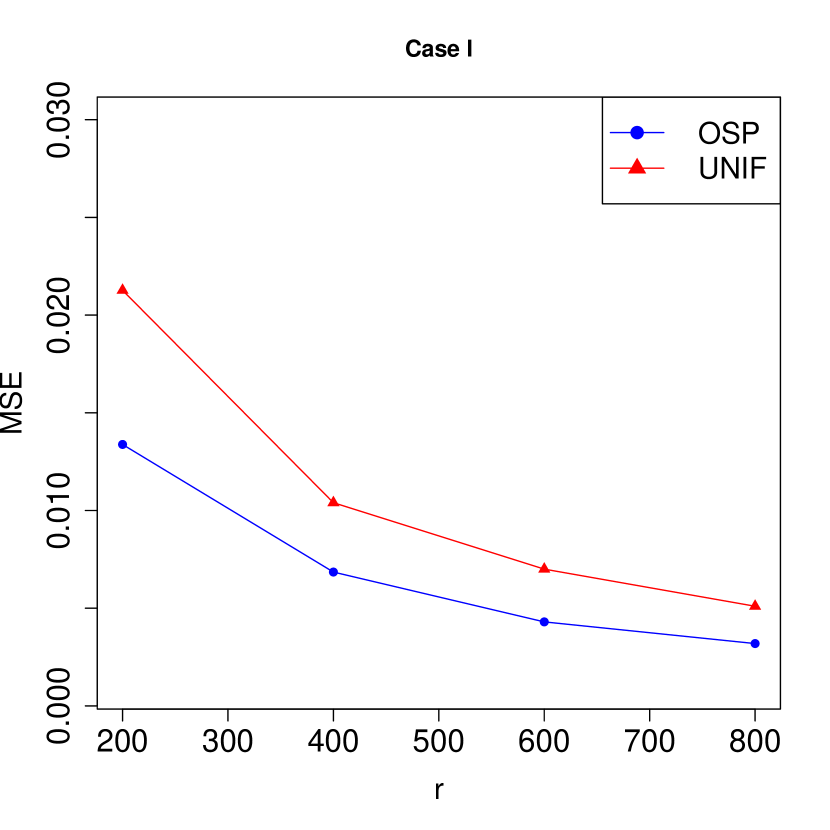
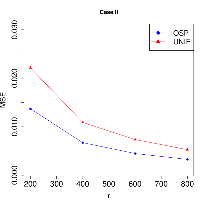
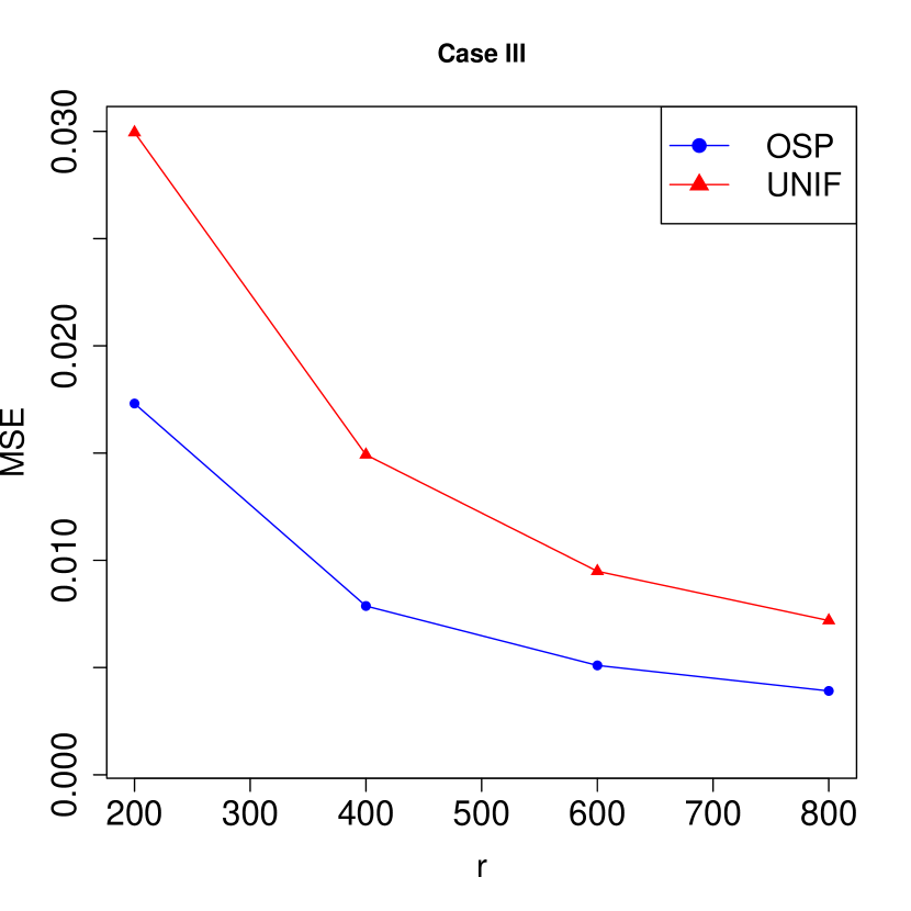
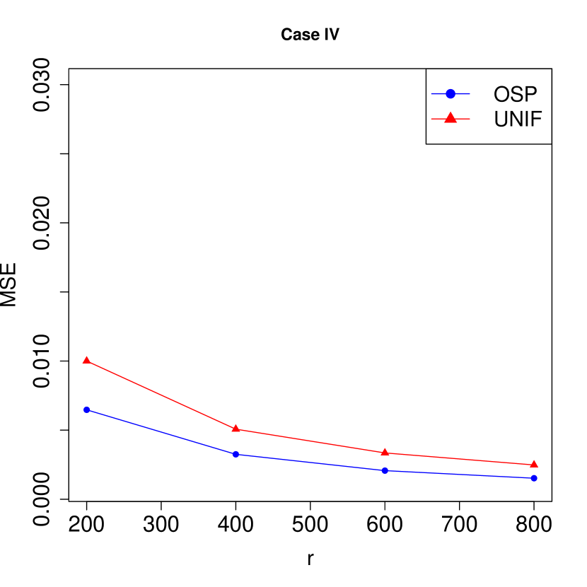
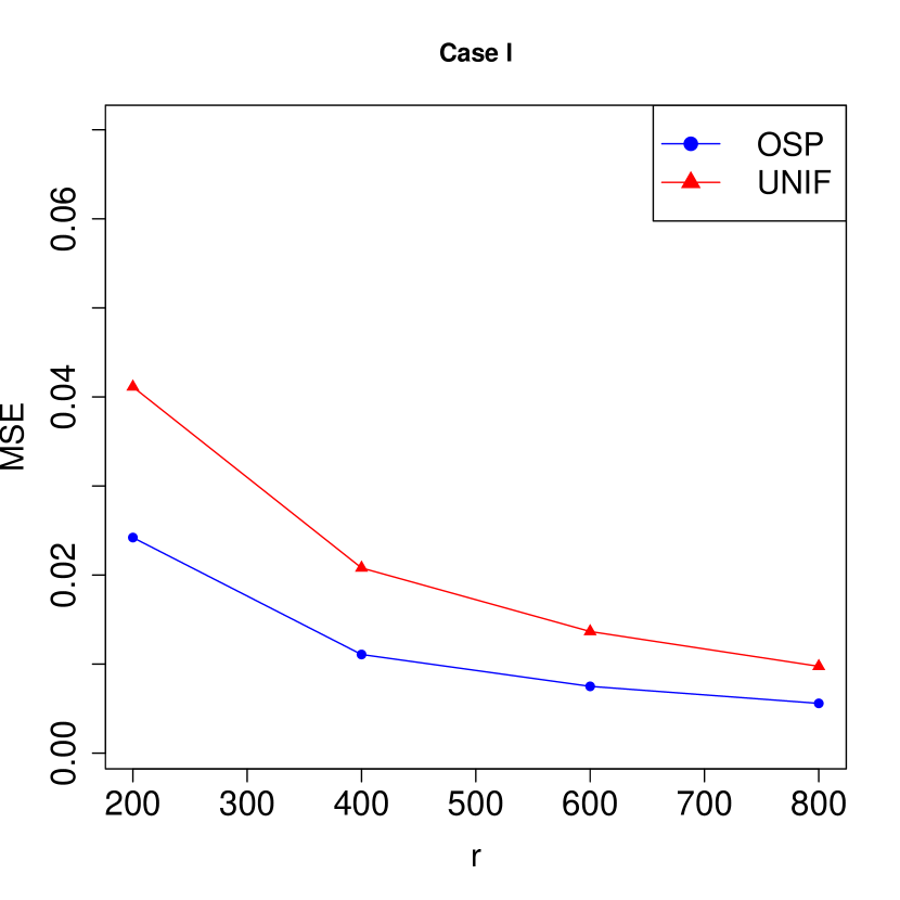
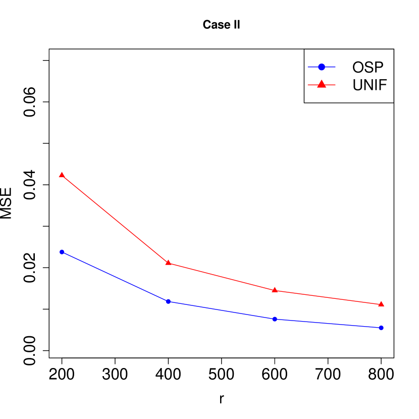
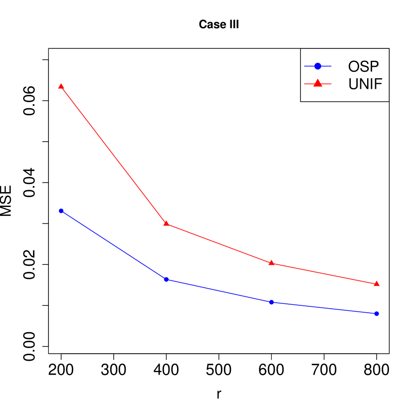
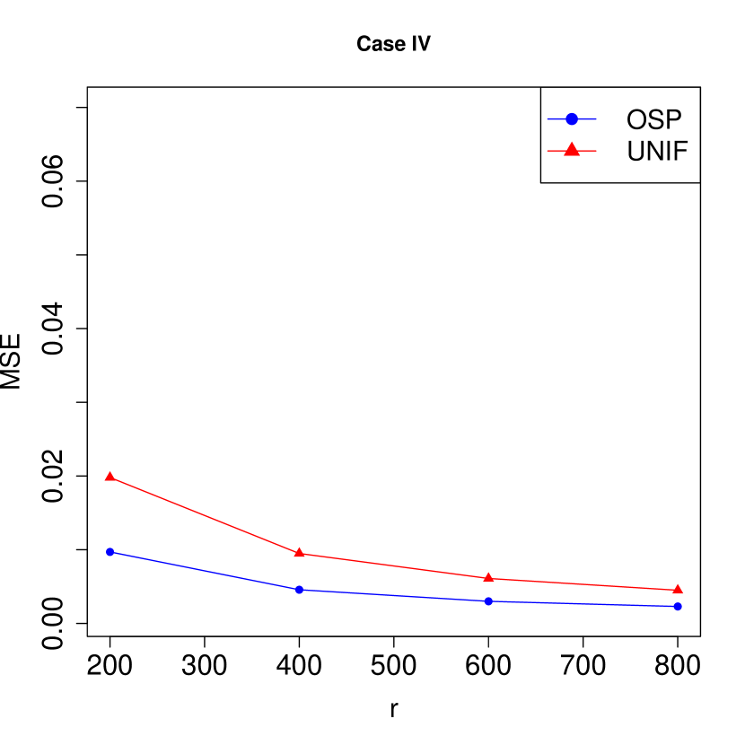
We compared the distributed optimal Poisson subsampling estimator from Algorithm 2 (“OSP estimator”) with the estimator from the distributed uniform Poisson subsampling method (“UNIF estimator”) and set $\delta=0.1$. The estimation results for $\beta_{1}$ were presented in Tables 1 and 2, including the empirical biases (Bias), the mean estimated standard errors (SE), the empirical standard errors (ESE), and the empirical 95% coverage probability (CP). The estimation results for other regression coefficients were similar and were therefore omitted. One can tell both the OSP and UNIF yielded unbiased estimation. The SE and ESE were close to each other, and the coverage probabilities agreed well with the asymptotic nomial level. As the sampling size increased, both the SE and ESE became smaller. With the same subsample sizes, however, the OSP yielded smaller Biases and ESE as compared to the UNIF. In addition, we calculated the empirical mean squared error (MSE), defined by

$${\rm MSE}(\breve{\bm{\beta}}_{\mbox{\tiny\rm DSE}})=\frac{1}{500}\sum_{b=1}^{500}\|\breve{\bm{\beta}}_{\mbox{\tiny\rm DSE}}^{(b)}-\bm{\beta}_{0}\|^{2},$$

where $\breve{\bm{\beta}}_{\mbox{\tiny\rm DSE}}^{(b)}$ is the estimate from the $b$th subsample. Figures 1 and 2 present the MSEs of OSP and UNIF, from which we see the OSP had lower MSEs than UNIF in all scenarios.

Table 1: Simulation results of the subsample estimator $\breve{\beta}_{1}$ with CR = $20\%$.

			OSP					UNIF
	$r_{k}$		Bias	ESE	SE	CP		Bias	ESE	SE	CP
Case I	200		0.0043	0.0541	0.0563	0.960		0.0014	0.0689	0.0709	0.958
	400		0.0005	0.0391	0.0392	0.952		0.0017	0.0457	0.0500	0.972
	600		0.0006	0.0294	0.0318	0.966		0.0001	0.0381	0.0408	0.978
	800		0.0013	0.0258	0.0274	0.964		$4\times 10^{-5}$	0.0321	0.0353	0.972
Case II	200		0.0122	0.0527	0.0540	0.946		-0.0028	0.0641	0.0685	0.958
	400		0.0076	0.0378	0.0376	0.946		-0.0027	0.0455	0.0481	0.960
	600		0.0057	0.0298	0.0305	0.948		-0.0005	0.0371	0.0392	0.968
	800		0.0051	0.0261	0.0264	0.936		-0.0003	0.0308	0.0339	0.968
Case III	200		0.0129	0.0692	0.0695	0.944		0.0047	0.0858	0.1004	0.964
	400		0.0054	0.0468	0.0482	0.944		-0.0012	0.0626	0.0696	0.956
	600		0.0040	0.0377	0.0390	0.958		-0.0029	0.0489	0.0583	0.972
	800		0.0021	0.0337	0.0338	0.942		-0.0024	0.0418	0.0504	0.966
Case IV	200		0.0090	0.0380	0.0407	0.960		-0.0001	0.0472	0.0536	0.964
	400		0.0037	0.0275	0.0280	0.944		0.0002	0.0328	0.0378	0.970
	600		0.0017	0.0212	0.0227	0.956		0.0028	0.0259	0.0307	0.972
	800		0.0008	0.0189	0.0196	0.966		0.0023	0.0214	0.0263	0.970

Table 2: Simulation results of the subsample estimator $\breve{\beta}_{1}$ with CR = $60\%$.

			OSP					UNIF
	$r_{k}$		Bias	ESE	SE	CP		Bias	ESE	SE	CP
Case I	200		0.0087	0.0735	0.0733	0.960		0.0052	0.0934	0.0980	0.960
	400		0.0031	0.0492	0.0511	0.970		0.0019	0.0658	0.0687	0.966
	600		0.0022	0.0421	0.0415	0.934		0.0015	0.0522	0.0559	0.972
	800		0.0015	0.0347	0.0358	0.948		0.0017	0.0451	0.0484	0.970
Case II	200		0.0068	0.0661	0.0687	0.972		-0.0011	0.0923	0.0927	0.950
	400		0.0034	0.0444	0.0476	0.956		-0.0027	0.0634	0.0649	0.962
	600		0.0031	0.0355	0.0386	0.970		-0.0022	0.0524	0.0530	0.946
	800		0.0032	0.0311	0.0334	0.966		-0.0023	0.0452	0.0459	0.954
Case III	200		0.0260	0.1044	0.1089	0.952		0.0117	0.1389	0.1420	0.952
	400		0.0088	0.0736	0.0754	0.946		0.0122	0.0948	0.0979	0.956
	600		0.0044	0.0604	0.0614	0.962		0.0094	0.0793	0.0799	0.948
	800		0.0041	0.0510	0.0531	0.966		0.0065	0.0695	0.0692	0.944
Case IV	200		0.0092	0.0446	0.0469	0.952		-0.0062	0.0650	0.0922	0.960
	400		0.0043	0.0306	0.0324	0.966		-0.0029	0.0451	0.0536	0.964
	600		0.0033	0.0252	0.0261	0.948		-0.0032	0.0363	0.0432	0.968
	800		0.0034	0.0214	0.0224	0.948		-0.0025	0.0301	0.0370	0.972

Figure 1: The MSEs of UNIF and OSP estimators with CR=20%.

Figure 2: The MSEs of UNIF and OSP estimators with CR=60%.

4.2 Real-world Data Example

In this section, we apply the proposed distributed Poisson subsampling estimation procedure to a large set of USA airline data. There were 57,729,435 commercial flights that experienced arrival delays within the United States between October 1987 and April 2008. The failure time is defined as the duration, measured in minutes, from the scheduled arrival time to the actual arrival time. We treated the 33,142,872 flights of delayed times within 15 minutes as censoring, with the CR approximately 42.6%. For computational efficiency, we divided the full samples by decades, and obtained $n_{1}=27,221,837$ for data between 1987 and 1997, and $n_{2}=30,507,598$ for data between 1998 and 2008. In the Cox model, we specified two covariates $X_{ik,1}$ and $X_{ik,2}$ ($k=1,2$), which represent departure status (0 for on or ahead of scheduled time and 1 for delayed departure) and distance (a continuous variable measured in thousands of miles), respectively. It was defined $\mathbf{X}_{ik}=(X_{ik,1},X_{ik,2})^{\prime}$.

Table 3: The Bias and (ESE, SE) for subsample estimates in real data.

			OSP	UNIF
$r_{k}=200$	$\beta_{1}$		0.0165 (0.1305, 0.1238)	0.0118 (0.1395, 0.1374)
	$\beta_{2}$		0.0072 (0.1016, 0.1036)	0.0219 (0.1369, 0.1337)
$r_{k}=400$	$\beta_{1}$		0.0105 (0.0908, 0.0867)	0.0111 (0.0987, 0.0966)
	$\beta_{2}$		0.0125 (0.0733, 0.0719)	0.0174 (0.0954, 0.0939)
$r_{k}=600$	$\beta_{1}$		0.0115 (0.0747, 0.0705)	0.0069 (0.0776, 0.0787)
	$\beta_{2}$		0.0146 (0.0588, 0.0585)	0.0171 (0.0744, 0.0766)
$r_{k}=800$	$\beta_{1}$		0.0100 (0.0618, 0.0609)	0.0084 (0.0663, 0.0681)
	$\beta_{2}$		0.0105 (0.0487, 0.0505)	0.0158 (0.0648, 0.0663)

For analysis, we consider the OSP estimator with $\delta=0.1$ and the UNIF estimator, where the pilot subsample size is chosen as $r_{0k}=200$. The values of $r_{k}$ are set to 200, 400, 600, and 800. Table 3 presents the Bias, SE and ESE of subsample-based estimates based on 500 subsamples, where Bias is calculated by the difference between the subsampling estimator and the complete data estimator. Based on the findings presented in Table 3, it can be observed that both estimates derived from subsampling techniques exhibit consistency as the subsample size increases. Additionally, the standard error of the OSP estimator is significantly smaller than that of the UNIF estimator, which confirms the optimality of OSP as established by Theorem 2.

5 Concluding Remarks

In this paper, we proposed a distributed Poisson subsampling approach for the Cox model in massive data settings. Our approach can alleviate the computational burden and ensure data privacy during the communication of multiple datasets. For practical inferences, the asymptotic property of the proposed estimator was provided. The simulation study demonstrated that the proposed approach is effective, and the methodology was applied to analyze a large dataset from the U.S. airlines.

There are two possible directions for future research. First, we employed time-independent covariates only but in reality, the covariates can be time-dependent. It is desirable to extend the proposed approach to incorporate time-dependent covariates. Second, besides inferences, the proposed framework lays the foundation for handling other time-consuming tasks with massive datasets, such as variable selection. Although it has been well known variable selection with big data is extremely time-consuming, the proposed subsampling technique offers a promising approach to alleviate the computational load. Therefore, it would be intriguing to explore the potential of combine the distributed Poisson subsampling estimation approach for Cox models with adaptive Lasso Zhang and Lu (2007) and SCAD Fan and Li (2002).

References

• Andersen and Gill (1982) Andersen, P. K. and Gill, R. D. (1982). Cox’s regression model for counting processes: A large sample study. The Annals of Statistics 10, 4, 1100–1120.
• Atkinson et al. (2007) Atkinson, A., Donev, A., and Tobias, R. (2007). Optimum Experimental Designs, with SAS. Oxford: Oxford University Press.
• Cox (1972) Cox, D. R. (1972). Regression models and life-tables (with discussions). Journal of the Royal Statistical Society, Series B 34, 187–220.
• Cox (1975) Cox, D. R. (1975). Partial likelihood. Biometrika 62, 2, 269–276.
• Fan and Li (2002) Fan, J. and Li, R. (2002). Variable selection for cox’s proportional hazards model and frailty model. Annals of Statistics 30, 74–99.
• Fang et al. (2017) Fang, E. X., Ning, Y., and Liu, H. (2017). Testing and confidence intervals for high dimensional proportional hazards models. Journal of the Royal Statistical Society: Series B (Statistical Methodology) 79, 5, 1415–1437.
• Han et al. (2022) Han, L., Hou, J., Cho, K., Duan, R., and Cai, T. (2022). Federated adaptive causal estimation (face) of target treatment effects. arXiv:2112.09313v3 .
• Han et al. (2020) Han, L., Tan, K. M., Yang, T., and Zhang, T. (2020). Local uncertainty sampling for large-scale multiclass logistic regression. The Annals of Statistics 48, 1770–1788.
• Huang et al. (2013) Huang, J., Sun, T., Ying, Z., Yu, Y., and Zhang, C.-H. (2013). Oracle inequalities for the lasso in the cox model. The Annals of Statistics 41, 3, 1142–1165.
• Keret and Gorfine (2023) Keret, N. and Gorfine, M. (2023). Analyzing big EHR data-optimal cox regression subsampling procedure with rare events. Journal of the American Statistical Association DOI: 10.1080/01621459.2023.2209349.
• Lin and Xi (2011) Lin, N. and Xi, R. (2011). Aggregated estimating equation estimation. Statistics and Its Interface 4, 73–83.
• Wang and Ma (2021) Wang, H. and Ma, Y. (2021). Optimal subsampling for quantile regression in big data. Biometrika 108, 99–112.
• Wang et al. (2019) Wang, H., Yang, M., and Stufken, J. (2019). Information-based optimal subdata selection for big data linear regression. Journal of the American Statistical Association 114, 525, 393–405.
• Wang et al. (2018) Wang, H., Zhu, R., and Ma, P. (2018). Optimal subsampling for large sample logistic regression. Journal of the American Statistical Association 113, 522, 829–844.
• Wang et al. (2022) Wang, J., Zou, J., and Wang, H. (2022). Sampling with replacement vs poisson sampling: a comparative study in optimal subsampling. IEEE Transactions on Information Theory 68, 6605–6630.
• Wang and Zhang (2022) Wang, T. and Zhang, H. (2022). Optimal subsampling for multiplicative regression with massive data. Statistica Neerlandica 76, 418–449.
• Xiong et al. (2023) Xiong, R., Koenecke, A., Powell, M., Shen, Z., Vogelstein, J. T., and Athey, S. (2023). Federated causal inference in heterogeneous observational data. Statistics in Medicine DOI: 10.1002/sim.9868.
• Yang et al. (2022) Yang, Z., Wang, H., and Yan, J. (2022). Optimal subsampling for parametric accelerated failure time models with massive survival data. Statistics in Medicine 41, 5421–5431.
• Yao and Wang (2021) Yao, Y. and Wang, H. (2021). A review on optimal subsampling methods for massive datasets. Journal of Data Science 19, 151–172.
• Yao et al. (2021) Yao, Y., Zou, J., and Wang, H. (2021). Optimal poisson subsampling for softmax regression. Journal of Systems Science and Complexity , accepted.
• Yu et al. (2023) Yu, J., Ai, M., and Ye, Z. (2023). A review on design inspired subsampling for big data. Statistical Papers 1–44.
• Yu et al. (2022) Yu, J., Wang, H., Ai, M., and Zhang, H. (2022). Optimal distributed subsampling for maximum quasi-likelihood estimators with massive data. Journal of the American Statistical Association 117, 265–76.
• Zhang and Wang (2021) Zhang, H. and Wang, H. (2021). Distributed subdata selection for big data via sampling-based approach. Computational Statistics & Data Analysis 153, 107072.
• Zhang et al. (2023) Zhang, H., Zuo, L., Wang, H., and Sun, L. (2023). Approximating partial likelihood estimators via optimal subsampling. Journal of Computational and Graphical Statistics DOI: 10.1080/10618600.2023.2216261.
• Zhang and Lu (2007) Zhang, H. H. and Lu, W. (2007). Adaptive lasso for cox’s proportional hazards model. Biometrika 94, 691–703.
• Zuo et al. (2021) Zuo, L., Zhang, H., Wang, H., and Sun, L. (2021). Optimal subsample selection for massive logistic regression with distributed data. Computational Statistics 36, 2535–2562.