Conformal inference for regression on Riemannian Manifolds

Abstract

Regression on manifolds, and, more broadly, statistics on manifolds, has garnered significant importance in recent years due to the vast number of applications for this type of data. Circular data is a classic example, but so is data in the space of covariance matrices, data on the Grassmannian manifold obtained as a result of principal component analysis, among many others. In this work we investigate prediction sets for regression scenarios when the response variable, denoted by $Y$, resides in a manifold, and the covariable, denoted by $X$, lies in Euclidean space. This extends the concepts delineated in [Lei and Wasserman, 2014] to this novel context. Aligning with traditional principles in conformal inference, these prediction sets are distribution-free, indicating that no specific assumptions are imposed on the joint distribution of $(X,Y)$, and they maintain a non-parametric character. We prove the asymptotic almost sure convergence of the empirical version of these regions on the manifold to their population counterparts. The efficiency of this method is shown through a comprehensive simulation study and an analysis involving real-world data.

1 Introduction

Conformal prediction is a powerful set of statistical tools that operates under minimal assumptions about the underlying model. It is primarily used to construct confidence sets that are applicable to a diverse range of problems in fields such as machine learning and statistics.

Conformal prediction is unique in its ability to construct prediction regions that guarantee a specified level of coverage for finite samples, irrespective of the distribution of the data. This is particularly crucial in high-stakes decision-making scenarios where maintaining a certain level of coverage is critical.

Unlike other methods, conformal prediction does not require strong assumptions about the sample distribution, such as normality. The aim is to construct prediction regions as small as possible to yield informative and precise predictions, enhancing the tool’s utility in various applications.

The approach was first proposed by Vovk, Gammerman, and Shafer in the late 1990s, as referenced in [Vovk et al., 1998]. Since its inception, it has been the subject of intense research activity. Originally formulated for binary classification problems, the method has since been expanded to accommodate regression, multi-class classification, functional data, functional time series, and anomaly detection, among others. Several applications of this method can be found in the book [Balasubramanian et al., 2014].

In the context of regression, conformal prediction has proven to be efficient in constructing prediction sets, as evidenced by works such as [Lei and Wasserman, 2014], [Wäschle et al., 2014], and [Kuleshov et al., 2018]. To enhance the performance of these prediction sets, particularly to decrease the length of prediction intervals (when the output is one-dimensional), a combination of conformal inference and quantile regression was proposed in [Romano et al., 2019]. In [Fong and Holmes, 2021], computationally efficient conformal inference methods for Bayesian models were proposed.

The method has also been extended to functional regression, where the predictors and responses are functions, rather than vectors, see for instance [Lei et al., 2015], [Fontana et al., 2020] and [Diquigiovanni et al., 2022]. In this case, the prediction regions take the form of functional envelopes that have a high probability of containing the true function.

In the field of classification, conformal prediction has been employed to tackle a broad spectrum of problems. These include image classification, as in [Lei, 2014], and text classification, as in [Vovk et al., 2005]. For multi-class classification, a prevalent approach is to create prediction sets that have a high likelihood of encompassing the correct class. This can be realized via the use of ‘Venn prediction sets’, as outlined in [Liu and Wasserman, 2016]. These sets partition the label space into overlapping regions, each one corresponding to a distinct class.

In summary, conformal prediction provide powerful statistical tools and has been successfully applied to a wide range of problems in machine learning, statistics, and related fields. Its main advantage is its ability to provide distribution-free prediction regions that can be used in the presence of any underlying distribution of the data. As this field of research continues to evolve, it is expected to find even more applications in the future.

1.1 Conformal inference on manifolds

In the regression framework, when the output $Y$ belongs to a Riemannian manifold, several arguments used in Euclidean conformal inference are not straightforwardly extendable. For instance, the Frechet mean on the manifold can be defined, but it does not always exist nor is it necessarily unique. Moreover, formulating a regression model on the manifold is not easy because of the absence of any additive structure, although there have been recent advances in this area (see for instance [Petersen and Müller, 2019]).

However, there are certain types of data that, due to their inherent characteristics, must be treated as data on manifolds. A prominent example of this are covariance matrices (for instance, the volatility of a portfolio, see [Best, 2010] and [Huang and Kou, 2014]), which are data in the manifold of positive definite matrices (see [Cholaquidis et al., 2023a]). Vectorcardiograms are condensed into data on the Stiefel manifold (see [Cholaquidis et al., 2023b]). The outcome of performing a principal component analysis results in data on the Grassmannian manifold (see [Hong et al., 2016]). Wind measurements can be represented as data on the cylinder (see [Cholaquidis et al., 2022]).

Applications in image analysis are developed in [Pennec et al., 2019] and more generally in machine learning in [Guigui et al., 2023]

In our paper we have adopted the approach of constructing confidence bands used by [Lei and Wasserman, 2014]. In this method, the confidence band is constructed through density estimators, which, as demonstrated in [Cholaquidis et al., 2022], can be naturally extended to manifolds, including those with boundaries. Although several of the arguments we use in the proofs are adaptations of the ideas presented in [Lei and Wasserman, 2014], many others require particular geometric considerations. For example, manifolds with boundaries have the drawback that classical density estimators (kernel estimators, for example) do not converge uniformly over the entire manifold, but only at points far from the boundary. As far as our knowledge extends, the present paper is the first to extend conformal inference ideas to manifolds.

2 Conformal prediction based on density estimation

In the following, $\aleph_{n}=\{(X_{i},Y_{i}):i=1,\dots,n\}$ will denote an i.i.d. sample of $(X,Y)$ with distribution $P$, where $X\in\mathbb{R}^{d}$ and $Y\in M$, with $(M,\rho)$ being a compact $\ell$-dimensional submanifold of $\mathbb{R}^{D}$. We denote by $P_{X}$ the marginal distribution of $X$ and by $\text{supp}(P_{X})$ its support. We denote the volume measure on $M$ by $\nu$ and use $|\cdot|$ to denote the Euclidean norm on $\mathbb{R}^{D}$. We denote by $\mu$ the $d$-dimensional Lebesgue measure in $\mathbb{R}^{d}$.

The following definition is taken from [Lei and Wasserman, 2014]:

Definition 1.

Given $\alpha\in(0,1)$, and $x$ in the support of $P_{X}$, a set $C_{n}(x)\subset M$ is said to be conditionally valid if

$$\mathbb{P}\big{(}Y\in C_{n}(x)\mid X=x\big{)}\geq 1-\alpha.$$

This definition captures the notion of a set of possible values of $Y$ that provides a specified level of coverage for a given imput $x$.

We will also define the population counterparts of $C_{n}$ (the “conditional oracle band” as it is called in [Lei and Wasserman, 2014]),

$$C_{P}(x)=\{y:p(y|x)\geq t^{\alpha}(x)\}$$ (1)

where $t^{\alpha}(x)$ satisfies

$$\int\mathbbm{1}_{\{p(y|x)\geq t^{\alpha}(x)\}}p(y|x)dy=1-\alpha.$$ (2)

As is shown in lemma 1 of [Lei and Wasserman, 2014], non-trivial finite sample conditional validity for all $x$ in the support of $P_{X}$ is impossible for a continuous distribution. To overcome this limitation, the following notion of local validity will be introduced.

Definition 2.

Let $\mathcal{A}=\{A_{j}:j\geq 1\}$ be a partition of $\textrm{supp}(P_{X})$. A prediction band $C_{n}$ is locally valid with respect to $\mathcal{A}$ if

$$\mathbb{P}(Y_{n+1}\in C_{n}(X_{n+1})|X_{n+1}\in A_{j})\geq 1-\alpha\text{ for all }j\text{ and all }P.$$ (3)

Whenever $A_{k}\in\mathcal{A}$, we will write $p(y|A_{k})$ for the conditional density, w.r.t. $\mu$, of $Y$ given $X\in A_{k}$.

2.1 Assumptions

We will now us the set of assumptions that we will require. H1 to H4 are also imposed in [Lei and Wasserman, 2014]. Hypotheses H0 and H4 are imposed to guarantee the uniform convergence of the kernel-based density estimator of the conditional density.

• $M$ is a $\mathcal{C}^{2}$ submanifold, and if $\partial M\neq\emptyset$, then $\partial M$ is also a $\mathcal{C}^{2}$ submanifold.

• The joint distribution $P$ has a density $p_{X,Y}(x,y)$ w.r.t. $\mu\times\nu$, and the marginal distribution $P_{X}$ has a density $p_{X}$ (w.r.t. $\mu$). We denote by $p(y|x)=p_{X,Y}(x,y)/p_{X}(x)$ the conditional density, where $p(y|x)=0$ if $p_{X}(x)=0$.

• $p_{X}$ is such that that there exist $b_{1},b_{2}$ such that $0<b_{1}\leq p_{X}(x)\leq b_{2}<\infty$ for all $x$ in the support of $X$.

• $p(y|x)$ is Lipschitz continuous as a function of $x$, i.e., there exists a constant $L>0$ such that $|p(\cdot|x)-p(\cdot|x^{\prime})|_{\infty}\leq L|x-x^{\prime}|$.

• There are positive constants $\epsilon_{0}$, $\gamma$, $c_{1}$, and $c_{2}$ such that for all $x$ in the support of $X$,

  $$c_{1}\epsilon^{\gamma}\leq P(\{y:|p(y|x)-t_{x}^{\alpha}|<\epsilon\}|X=x)\leq c_{2}\epsilon^{\gamma},$$

  for all $\epsilon\leq\epsilon_{0}$, where $t_{x}^{\alpha}$ is the $\alpha$-quantile of the distribution of $p(y|x)$. Moreover $\inf_{x}t_{x}^{(\alpha)}\geq t_{0}>0$.

• $p(y|A_{k})$ is $\mathcal{C}^{4}$.

These assumptions impose a regularity on the joint and conditional densities of the data, as well as on the geometry of the submanifold $M$. In particular, the assumption of Lipschitz continuity H3 ensures that small changes in the input $x$ lead to small changes in the output $y$, while H4 ensures that $p(y|x)$ is well behaved, and does not exhibit extreme behavior for any input $x\in[0,1]^{d}$. These assumptions play a crucial role in the development and analysis of conformal prediction methods.

3 Locally valid bands

In this section, we introduce a slightly modified version of the estimated local marginal density $\hat{p}^{(x,y)}(v|A_{k})$ and of the local conformity rank $\pi_{n,k}(x,y)$ originally introduced in [Lei and Wasserman, 2014]. We make the assumption that $\textrm{supp}(P_{X})=[0,1]^{d}$, and that $\mathcal{A}=\{A_{k},k=1,\dots,M\}$ is a finite partition of $[0,1]^{d}$ consisting of equilateral cubes with sides of length $w_{n}$.

Let $n_{k}=\sum_{i=1}^{n}\mathbbm{1}_{\{X_{i}\in A_{k}\}}$. Given a sequence $h_{n}\to 0$, a kernel function $K(\cdot):\mathbb{R}\to\mathbb{R}$, and $h_{n_{k}}$, we define

$$\hat{p}(v|A_{k})=\frac{1}{n_{k}h_{n_{k}}^{\ell}}\sum_{i=1}^{n}\mathbbm{1}_{\{X_{i}\in A_{k}\}}K\Bigg{(}\frac{||Y_{i}-v||}{h_{n_{k}}}\Bigg{)}.$$ (4)

We aim to prove that $\hat{p}(v|A_{k})$ provides a uniform estimate of $p(y|A_{k})$ across $v$ and $k$. To achieve this, we need to ensure that there are sufficiently many sample points in each $A_{k}$. This is guaranteed by lemma 9 of [Lei and Wasserman, 2014], which states that if we choose $w_{n}=(\log(n)/n)^{1/(d+2)}$, then, with probability one, for all $n$ large enough,

$$\forall k:\quad b_{1}nw_{n}^{d}/2\leq n_{k}\leq 3b_{2}nw_{n}^{2}/2.$$ (5)

Recall that $b_{1}$ and $b_{2}$ are as defined in Assumption H2. In what follows, we assume that $n$ is sufficiently large to ensure (5).

The corresponding augmented estimate, based on $\aleph_{n}\cup\{(x,y)\}$ is, for any $(x,y)\in A_{k}\times M$,

$$\hat{p}^{(x,y)}(v|A_{k})=\frac{n_{k}}{n_{k}+1}\hat{p}(v|A_{k})+\frac{1}{(n_{k}+1)h_{n_{k}}}K\Bigg{(}\frac{||y-v||}{h_{n_{k}}}\Bigg{)}.$$

For any $(X_{n+1},Y_{n+1})=(x,y)\in A_{k}\times M$, consider the following local conformity rank

$$\pi_{n,k}(x,y)=\frac{1}{n_{k}+1}\sum_{i=1}^{n+1}\mathbbm{1}_{\{X_{i}\in A_{k}\}}\mathbbm{1}_{\{\hat{p}^{(x,y)}(Y_{i}|A_{k})\leq\hat{p}^{(x,y)}(Y_{n+1}|A_{k})\}}.$$ (6)

As proved in proposition 2 of [Lei and Wasserman, 2014], the set

$$\hat{C}_{n}(x)=\{y:\pi_{n,k}(x,y)\geq\alpha\}$$ (7)

has finite sample local validity, i.e., it satisfies (3).

The following is the key theorem. Its proof is deferred to the Appendix. Note that the proof follows the ideas used to prove theorem 1 of [Cholaquidis et al., 2022]. It states that $p(y|A_{k})$ can be estimated uniformly by (4) for all $y$ that are far enough from the boundary of $M$. Additionally, this estimation can be made uniformly across all $k$. We assume, as in [Cholaquidis et al., 2022], that $K$ is a Gaussian kernel. This restriction is, as in [Cholaquidis et al., 2022], purely technical.

This result is of fundamental importance in conformal prediction, as it provides a way to estimate the conditional density of $Y$ given $A_{k}$ for any $k$ in a non-parametric way. In particular, it allows us to construct conformal prediction regions that are valid with a given level of confidence. However, we must be careful when estimating the density near the boundary of $M$, as the performance of the method may deteriorate due to lack of data or a poor estimate of the underlying density. Therefore, it is important to consider appropriate modifications of the method when working near the boundary, or to restrict the analysis to regions where the density can be estimated reliably.

Theorem 1.

Let $M\subset\mathbb{R}^{D}$ be a compact $\ell$-dimensional manifold satisfying H0. Let $M_{n}\subset M$ be a sequence of closed sets, and let $h_{n}\to 0$ be a sequence of bandwidths such that $nh_{n}^{\ell+3}/\log(n)\to\infty$. We assume that $c_{n}:=\inf_{x\in M_{n}}\rho(x,\partial M)\to 0$ is such that $h_{n}/c_{n}\to 0$ monotonically. Additionally, we assume that $p(y|A_{k})$ satisfies H5. Then, we have

$$\sup_{k}\sup_{x\in M_{n_{k}}}|\hat{p}(y|A_{k})-p(y|A_{k})|=o(h_{\gamma_{n}}/c_{\gamma_{n}})\quad\text{a.s.},$$ (8)

where $\gamma_{n}=\lfloor b_{1}nw_{n}^{d}/2\rfloor$.

The following theorem is the main result of our paper. It states that $\hat{C}_{n}(X_{i})$ consistently estimates $C_{P}(X_{i})$ uniformly for all $X_{i}\in\aleph_{n}$. The proof, which is deferred to the Appendix, see subsection 6.1, is based on some ideas from the proof of theorem 1 of [Lei and Wasserman, 2014]. Specifically, Lemma 1 and Lemma 3 are adapted from [Lei and Wasserman, 2014], while Lemma 2 is new and is required to adapt the proof of Lemma 3. Lemma 4 is the same as lemma 8 of [Lei and Wasserman, 2014]. Finally, the proof of Theorem 2 uses the adapted lemmas and considers separately the sample points that are close to $\partial M$ and those that are far from this boundary. The first set of points is shown to be negligible with respect to $\nu$ using techniques from geometric measure theory.

Theorem 2.

Assume H0 to H5. Let $\hat{C}_{n}(x)$ be given by (7) and $C_{P}(x)$ be given by (1). Let $w_{n}=(\log(n)/n)^{1/(d+2)}$ and $\gamma_{n}=\lfloor b_{1}nw_{n}^{d}/2\rfloor$. Then, for any $\lambda>0$, there exists an $A_{\lambda}>0$ such that, for $n$ large enough,

$$\mathbb{P}\Big{(}\sup_{X:(X,Y)\in\aleph_{n}}\nu(\hat{C}_{n}(X)\triangle C_{P}(X))>A_{\lambda}c_{\gamma_{n}}\Big{)}=O(n^{-\lambda}),$$

where $c_{\gamma_{n}}$ is such that $h_{\gamma_{n}}/c_{\gamma_{n}}^{2}\to 0$ and $h_{\gamma_{n}}\to 0$ such that $\gamma_{n}h_{\gamma_{n}}^{\ell+3}/\log(\gamma_{n})\to\infty$.

4 Simulation examples

4.1 Output on the sphere

We consider a regression model with output variable denoted by $Y_{i}$ defined on the unit sphere $S^{2}$. The input variable $X_{i}$ takes values in the interval $[-1,1]$. The model is given by the following probability distribution:

$$Y_{i}\sim\textrm{M}\left(\frac{\eta+\beta X_{i}}{\|\eta+\beta X_{i}\|},\kappa\right),\,i=1,2\ldots,400.$$

Here, M denotes the Von Mises–-Fisher distribution (see [Mardia et al., 2000]), and $X_{i}\sim\textrm{U}(-1,1)$ is an i.i.d. sample. For the simulation study, we set $\eta=(1,0,0)$, $\beta=(0,0,1)$, and $\kappa=200$.

To estimate the kernel density, we use the estimator given by Equation (4) with a bandwidth parameter $h=0.5$. Additionally, we partition the data into intervals $A_{k}=\left(-1+(k-1)/2,-1+k/2\right)$, where $k=1,\ldots,4$.

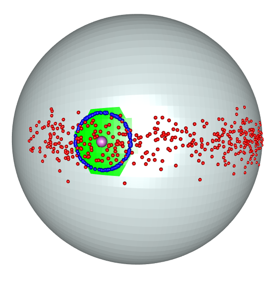
Using the proposed method, we obtain a $90\%$ confidence band $C_{400}(0)$, shown in green in Figure 1. In this particular case, the unobserved output was $Y=(1,0,0)$, which is illustrated in purple in Figure 1. Points belonging to the boundary of the theoretical confidence set 1 for $\alpha=0.1$ are displayed in blue.

Figure 1: Red: a sample $Y_{1},\ldots,Y_{400}$ on $S^{2}$. Green: the estimated $90\%$-confidence band for $Y$ if $x=0$. Purple: the point prediction for $x=0$, which is $y=(1,0,0)$. Blue dots belong to the boundary of the theoretical confidence band (1) for $\alpha=0.1$.

4.2 Output in a Stiefel manifold.

It is common to summarize information from a set of variables using Principal Component Analysis (PCA) or Factor Analysis. This approach is frequently employed in constructing indices within the social sciences, as demonstrated by Vyas (2006). Subsequently, researchers often attempt to explain these indices using other covariates. To illustrate this scenario, we provide a ‘toy example’ using simulations.

We will define a regression model whose output lies on the Stiefel Riemannian manifold $SO(3,2)$, represented by two-dimensional orthonormal vectors in $\mathbb{R}^{3}$. The construction of the regression is as follows.

The input variable, denoted by $X$, is uniformly distributed on the interval $[0,1]$. For each value of $X$, we sample $400$ points from a 3-dimensional Gaussian distribution centered at the origin $(0,0,0)$. The covariance matrix of this Gaussian distribution has eigenvalues $2$, $1$, and $1/2$, along with the corresponding eigenvectors $(2+X,2+2X,2-X)$, $(-2+X,2-3X,-2+X)$, and $(1,0,0)$, respectively.

After generating these $400$ points for each value of $X$, the output $Y\in SO(3,2)$ is obtained by applying a PCA to these points and retaining only the first two principal directions. To conduct the simulations analysis, we sample $500$ points, denoted by $X_{1},\dots,X_{500}$.

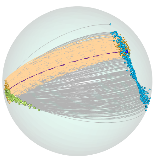
In Figure 2, we present a sample of $500$ output values, represented as gray arcs. The specific output value $y_{0.1}\in SO(3,2)$, corresponding to the input $X=0.1$, is depicted as a purple dotted arc.

To estimate the kernel density, we use the estimator given by Equation (4), with a bandwidth parameter $h=1$. Additionally, we divide the data into intervals $A_{k}=\left((k-1)/5,k/5\right)$, where $k=1,\ldots,5$. It is important to note that the $SO(3,2)$ data are embedded in $\mathbb{R}^{6}$ ($D=6$), and we consider the Euclidean distance in this space. The dimension of the submanifold in this case is $\ell=3$.

To visualize the confidence band, we draw $10000$ points within $SO(3,2)$. The points falling within the confidence band are highlighted in orange in Figure 2.

Figure 2: A uniform sample of 10000 points in the $95\%$ confidence band (orange arcs) for $Y\in SO(3,2)$ if $x=0.1$. The sample value for $x=0.1$ is the $3\times 2$ matrix, $y_{x}$, whose first column is $(0.62,0.5,0.6)$ and second column is $(-0.3,0.86,-0.44)$, which is depicted in purple. The observations are represented by gray arcs in the sample in the output.

5 Real-data example

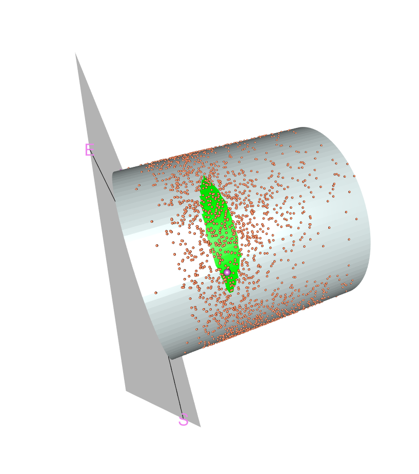
In this example, the objective is to predict the wind intensity, $R$, and direction, $\theta$, at a meteorological station in Uruguay from the same data at a nearby station. That is, the regression has values from one cylinder $\mathcal{C}$ in $\mathbb{R}^{3}$ (i.e., $\mathcal{C}=S^{1}\times\mathbb{R}^{+}$) to another. We will study the behavior of extreme and non-extreme winds (between 0 and 20 m/s). From the measurements obtained at the Laguna del Sauce Weather Station, Maldonado (Station 1), we want to construct prediction bands for the winds at the weather station located at the Carrasco International Airport, Montevideo (Station 2). The distance between the two stations is 84 km. The study period is 2008–2016 in the months of July. Measurements were recorded every hour. Only those records in which both stations are in operation are considered in the base ($5362$ records).

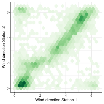
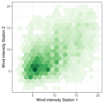
Figures 3 and 4 show that there is a correlation in both wind direction and intensity between the two stations. The $\xi$-correlation, see [Chatterjee, 2021], between the intensities is $0.45$. In the case of the directions, the angular correlation is $0.63$. The angular correlation is the linear correlation between the variables $\sin\left(\theta_{1}-\bar{\theta}_{1}\right)$ and $\sin\left(\theta_{2}-\bar{\theta}_{2}\right)$, see [Jammalamadaka and Sarma, 1988].

Figure 3: Scatter plot between the angular directions (in radians) of the winds recorded at Station 1 and Station 2 in the months of July between 2008 and 2016.

Figure 4: Scatter plot between the intensities (in m/s) of the winds recorded at Station 1 and Station 2 in the months of July between 2008 and 2016.

In this example, the partition is

$$A_{i,j}=\left\{(\theta,R)\in\mathcal{C}:\theta\in[i\frac{\pi}{4},(i+1)\frac{\pi}{4}]\textrm{ and }R\in[4j,4(j+1)]\right\}$$

with $i=0,1,\ldots,7$ and $j=0,1,\ldots,4$. For the kernel density estimator we choose $h_{k}=0.4$.

Figure 5 shows the confidence band (at 80%) obtained by our method for $(\theta_{1},R_{1})=(2.3\textrm{ radians},5.1\textrm{ m/s})$. This was recorded at Station 1 on 2008-07-01 at 7 pm. On the same date and time the data recorded at Station 2 were $(\theta_{2},R_{2})=(2.4\textrm{ radians},6.6\textrm{ m/s})$ (point depicted in purple in Figure 5).

Figure 5: Plot of winds (not exceeding 20 m/s) at Station 2 in the months of July between 2008 and 2016 (red). The green area is the 80% confidence band for the data recorded at Station 1 of $(2.3\textrm{ radians},5.1\textrm{ m/s})$ on 2008-07-01 at 7 pm. The purple dot represents the wind recorded at the same time at Station 2 ($(\theta_{2},R_{2})=(2.4\textrm{ radians},6.6\textrm{ m/s})$).

6 Conclusions and future work

We position ourselves within the broad context of conformal inference, where the response variable takes values on a manifold, while the input resides in $\mathbb{R}^{d}$. In this setting, we extend the results of [Lei and Wasserman, 2014] while maintaining similar hypotheses. We have demonstrated that it is possible to consistently estimate the conditional oracle band $C_{P}(x)$. A crucial tool in our analysis is the almost sure uniform consistency of the classical kernel density estimator on manifolds, as established in [Cholaquidis et al., 2022]. Our findings are substantiated by a simulation study conducted on two manifolds, namely the sphere and the Stiefel manifold, as well as a real-data example involving the cylinder. Notably, in the case of the sphere, our method exhibits good performance when compared to the true theoretical band.
A challenge for the future would be to establish adequate similar results when the dimension of the Riemannian manifold is high. In this direction, it would be necessary to study the extension of other conformal inference algorithms to Riemannian manifolds.

Appendix

Proof of Theorem 1.

Since $n_{k}h_{n_{k}}^{\ell+1}/\log(n_{k})\to\infty$, then, from theorem 1 of [Cholaquidis et al., 2022], for all $\epsilon>0$, with probability one, for all $n$ large enough,

$$\frac{c_{n_{k}}}{h_{n_{k}}}\sup_{y\in M_{n_{k}}}|\hat{p}(y|A_{k})-p(y|A_{k})|\leq\epsilon$$ (9)

Note that the index $n_{0}$ for which (9) holds depends on the choice of $k$. However, from (5), we know that with probability one, $n_{k}\geq\gamma_{n}$ for all $k$ when $n$ is sufficiently large. Since $h_{n}/c_{n}\to 0$ monotonically, it follows that for all $k$, $c_{n_{k}}/h_{n_{k}}\leq c_{\gamma_{n}}/h_{\gamma_{n}}$. Hence, we can conclude that (8) holds for all $k$. This result is important because it implies that the estimation error is uniform across all partitions $A_{k}$, which is a key requirement for conformal prediction methods. ∎

6.1 Proof of Theorem 2

The proof of Theorem 2 is based on some technical lemmas. To state them, let us define $L_{x}(t)$ as the set of $y$ such that $p(y|x)\geq t$, and $L_{x}^{l}(t)$ as the set of $y$ such that $p(y|x)\leq t$. We also define $\hat{L}_{x}(t)$ and $\hat{L}_{k}^{l}(t)$ as the corresponding sets for $\hat{p}(\cdot|A_{k})$, given by (4).

Lemma 1.

Under the hypotheses of Theorem 1, assume also H0 to H3. Let $R_{n}(x)=\sup_{y\in M_{\gamma_{n}}}|\hat{p}(y|A_{k})-p(y|x)|$. Then, with probability one, for $n$ sufficiently large, we have

$$\sup_{x\in\textrm{supp}(P_{X})}R_{n}(x)\leq h_{\gamma_{n}}/c_{\gamma_{n}}+Lw_{n}\sqrt{d},$$ (10)

where $\gamma_{n}=\lfloor b_{1}nw_{n}^{d}/2\rfloor$ and $\inf_{x\in M_{\gamma_{n}}}\rho(x,\partial M)=c_{\gamma_{n}}$.

Proof.

From (5), we can assume that $n$ is large enough and such that for all $k$, $b_{1}nw_{n}^{d}\leq n_{k}\leq b_{2}nw_{n}^{d}$. From (8), we obtain with probability one for $n$ large enough,

$$\sup_{y\in M_{\gamma_{n}}}|\hat{p}(y|A_{k})-p(y|A_{k})|\leq h_{n_{k}}/c_{n_{k}}.$$ (11)

Using assumption H3 and (5), we have

$$\sup_{x\in\textrm{supp}(P_{X})}R_{n}(x) \leq\sup_{x\in\textrm{supp}(P_{X})}\sup_{y\in M_{\gamma_{n}}}|\hat{p}(y|A_{k})-p(y|x)|$$

$$\leq\sup_{x\in\textrm{supp}(P_{X})}\sup_{y\in M_{\gamma_{n}}}|\hat{p}(y|A_{k})-p(y|A_{k})|+\sup_{y\in M_{\gamma_{n}}}|p(y|A_{k})-p(y|x)|$$

$$\leq h_{n_{k}}/c_{n_{k}}+Lw_{n}|x-y|$$

$$\leq h_{\gamma_{n}}/c_{\gamma_{n}}+Lw_{n}\sqrt{d},$$

where the last inequality follows from (5) and the fact that

$$\inf_{x\in M_{\gamma_{n}},y\in M}|x-y|\geq\rho(M_{\gamma_{n}},\partial M).$$

Thus, we have shown (10). ∎

Lemma 2.

Assume H0 to H4. Let $w_{n}=(\log(n)/n)^{1/(d+2)}$, and assume that $\gamma_{n}$ and $h_{n}$ are as in Lemma 1. Then, there exists $C>0$ such that with probability one for $n$ large enough

$$\sup_{k}\|\hat{p}(\cdot|A_{k})\|_{\infty}\leq C.$$

Proof.

Recall that we are assuming $K$ to be a Gaussian kernel. We assume that $n$ is large enough so that (5) holds. Following the proof of theorem 1 of [Cholaquidis et al., 2022], we define

$$W_{j}(y)=(1/(n_{k}h_{n_{k}}^{\ell}))\mathbbm{1}_{\{X_{j}\in A_{k}\}}K(|Y_{j}-y|/h{n_{k}}),$$

$V_{j}(y)=W_{j}(y)-\mathbb{E}(W_{j}(y))$, and $S_{n}(y)=\sum_{j=1}^{n}V_{j}(y)$. Let $\eta>\ell+1$ and consider a covering ${B(p_{1},h^{\eta}),\dots,B(p_{l},h^{\eta})}$ of $M$. Then,

$$\sup_{y}|S_{n}(y)|\leq\max_{1\leq j\leq l}\sup_{y\in B(p_{j},h^{\eta})}\frac{1}{n_{k}h_{n_{k}}^{\ell}}|S_{n}(y)-S_{n}(p_{j})|+\\ \max_{1\leq j\leq l}\frac{1}{n_{k}h_{n_{k}}^{\ell}}|S_{n}(p_{j})|=I_{1}+I_{2}.$$ (12)

Since $K$ is Lipschitz, we have $I_{1}\leq ch^{\eta-\ell-1}$ for some constant $c>0$. Applying Bernstein’s inequality to $S_{n}(p_{j})$ for fixed $p_{j}$ and $A_{k}$, we get

$$\mathbb{P}\Big{(}\frac{1}{n_{k}h_{n_{k}}^{\ell}}|S_{n}(p_{j})|>\epsilon\Big{)}\leq c_{1}\exp(-c_{2}n_{k}h_{n_{k}}^{\ell}\epsilon^{2}),$$

where $c_{1}$ and $c_{2}$ are positive constants.

Then, if $\kappa_{n}=\lfloor 3b_{2}nw_{n}^{d}\rfloor$,

$$\mathbb{P}\Big{(}\sup_{k}\sup_{y}|S_{n}(y)|>\epsilon\Big{)}\leq c_{3}w_{n}^{-d}\exp(-c_{3}nw_{n}^{d}h_{\kappa_{n}}^{\ell}).$$

By the Borel–Cantelli lemma, it follows that $\sup_{k}\sup_{y}|S_{n}(y)|\to 0$ almost surely.

Next, we will bound $\sup_{y}\mathbb{E}(V_{j}(y))$. First, we bound $1/h_{n_{k}}^{\ell}\leq 1/h_{\gamma_{n}}^{\ell}$,

$$\mathbb{E}(V_{j}(y))=\mathbb{E}[\mathbb{E}(V_{j}(y)|X)]\leq\int_{[0,1]^{d}}\int_{M}\frac{1}{h_{\gamma_{n}}^{\ell}}K(\|z-y\|/h_{\kappa_{n}})p(z|x)\nu(dz)p_{X}(x)dx.$$

Since $p_{X}(x)$ and $p(z|x)$ are bounded for all $z$ and $x$, it is enough to bound from above

$$\sup_{y}\int_{M}\frac{1}{h_{\kappa_{n}}^{\ell}}K(\|z-y\|/h_{\gamma_{n}})\nu(dz),$$

which is bounded because we assumed that $K$ is a Gaussian kernel. ∎

Lemma 6 of [Lei and Wasserman, 2014] proves a slightly modified version of the following lemma.

Lemma 3.

Assume H0 to H5. Let $\gamma_{n}=\lfloor b_{1}nw_{n}^{d}/2\rfloor$, $h_{\gamma_{n}}\to 0$, and $M_{\gamma_{n}}\subset M$ be a sequence of closed sets such that $\inf_{x\in M_{\gamma_{n}}}\rho(x,\partial M)/h_{\gamma_{n}}\to\infty$. Then, for any $\lambda>0$, there exists $\xi_{2,\lambda}$ such that, for $n$ large enough,

$$\mathbb{P}\Bigg{(}\sup_{x\in\aleph_{n}}V_{n}(x)>\xi_{2,\lambda}w_{n}\Bigg{)}=O(n^{-\lambda})$$ (13)

where $V_{n}(x)=\sup_{t\geq t_{0}}|\hat{P}(L_{x}^{l}(t)|A_{k})-P(L_{x}^{l}(t)|x)|$. Here, $\hat{P}(\cdot|A_{k})$ is the empirical distribution of $Y|X\in A_{k}$, $t_{0}$ is given in H4, and $w_{n}=(\log(n)/n)^{1/(d+2)}$.

Proof.

We will provide a sketch of the proof of this lemma since it follows essentially the same idea used to prove lemma 6 of [Lei and Wasserman, 2014].

Let $x\in A_{k}$ be fixed. Note that ${L_{x}^{l}(t):t\geq t_{0}}$ is a nested class of sets with Vapnik–Chervonenkis dimension 2. Then, for all $B>0$ and $\lambda>0$,

$$\mathbb{P}\Bigg{(}\sup_{t}\Big{|}\hat{P}(L_{x}^{l}(t)|A_{k})-P(L_{x}^{l}(t)|A_{k})\Big{|}>B\sqrt{w_{n}}\Bigg{)}=O(n^{-\lambda}),$$

where we used that $w_{n}=(\log(n)/n)^{1/(d+2)}$. On the other hand,

$$|P(L_{x}^{l}(t)|A_{k})-P(L_{x}^{l}(t)|x)|\leq Lw_{n}\nu(L_{x}(t))\sqrt{d}\leq Lw_{n}\nu(L_{x}(t_{0}))\sqrt{d}\leq L\nu(M)\sqrt{d}w_{n}.$$

Let $x^{\prime}\in A_{k}$. Then

$$|\hat{P}(L^{l}_{x^{\prime}}|A_{k})-P(L^{l}_{x^{\prime}}(t)|x^{\prime})|\leq\|\hat{p}(\cdot|A_{k})\|_{\infty}\nu(L_{x}^{l}(t)\triangle L^{l}_{x^{\prime}}(t))+V_{n}(x)+|G_{x}(t)-G_{x^{\prime}}(t)|$$

where $G_{x}(t)=P(L_{x}^{l}(t)|x)$. From (30) in [Lei and Wasserman, 2014],

$$|G_{x}(t)-G_{x^{\prime}}(t)|\leq c_{3}w_{n}^{1\wedge\gamma}.$$

Here, $c_{3}$ is a positive constant and $\gamma$ is as in H4. From (29) in [Lei and Wasserman, 2014], $\nu(L_{x}^{l}(t)\triangle L^{l}_{x^{\prime}}(t))\leq c_{4}w_{n}^{\gamma}$ for some positive constant $c_{4}$. Lastly, $\sup_{k}\|\hat{p}(\cdot|A_{k})\|_{\infty}$ is bounded, for $n$ large enough, using Lemma 2. ∎

We recall lemma 8 of [Lei and Wasserman, 2014].

Lemma 4.

Fix $\alpha>0$, $t_{0}>0$ and $\epsilon>0$. Suppose that $p$ is a density function that satisfies H4, and $\hat{p}$ an estimator such that $\|\hat{p}-p\|_{\infty}<v_{1}$. Let $\hat{P}$ be a probability measure satisfying $\sup_{t\geq t_{0}}|\hat{P}(L^{l}(t))-P(L^{l}(t))|<v_{2}$. Define

$$\hat{t}^{\alpha}=\inf\{t\geq 0:\hat{P}(\hat{L}^{l}(tq))\geq\alpha\}.$$

Assume that $v_{1}$ and $v_{2}$ are sufficiently small so that $v_{1}+c_{1}^{1/\gamma}v_{2}^{1/\gamma}\leq t^{\alpha}-t_{0}$ and $c_{1}^{-1/\gamma}v_{2}^{1/\gamma}\leq\epsilon_{0}$ where $c_{1}$ and $\gamma$ are the constants given in H4. Then

$$|\hat{t}^{\alpha}-t^{\alpha}|\leq v_{1}+c_{1}^{-1/\gamma}v_{2}^{1/\gamma}$$

Moreover, for any $\tilde{t}^{\alpha}$ such that $|\tilde{t}^{\alpha}-\hat{t}^{\alpha}|\leq v_{3}$, if $2v_{1}+c_{1}^{1/\gamma}v_{2}^{1/\gamma}+v_{3}\leq\epsilon_{0}$, then there are constants $\xi_{1},\xi_{2}$ and $\xi_{3}$ such that $\nu(\hat{L}(\tilde{t}^{\alpha})\triangle L(t^{\alpha}))\leq\xi_{1}v_{1}+\xi_{2}v_{2}+\xi_{3}v_{3}$.

Proof of Theorem 2

In what follows we assume that $n$ is sufficiently large to satisfy (5). We will consider a sequence of compact sets $M_{n}\subset M$ such that $\inf_{x\in M_{n}}\rho(x,\partial M)=c_{n}>0$ and $\sup_{x\in\partial M}\rho(x,M_{n})\leq 2c_{n}$, where $c_{n}$ is chosen such that $h_{\gamma_{n}}/c_{\gamma_{n}}^{2}\to 0$.

Throughout the proof we denote by $k$ a generic positive constant. Write

$$\nu(\hat{C}_{n}(x)\triangle C(x))=\nu(\hat{C}_{n}(x)\triangle C(x)\cap M_{\gamma_{n}})+\nu\{\hat{C}_{n}(x)\triangle C(x)\cap(M\setminus M_{\gamma_{n}})\}$$

where $\gamma_{n}$ is as in Lemma 3 and $M_{\gamma_{n}}\subset M$ is a sequence of closed sets such that $\inf_{x\in M_{\gamma_{n}}}\rho(x,\partial M)=c_{\gamma_{n}}$ satisfies $h_{\gamma_{n}}/c_{\gamma_{n}}\to 0$.

We will first prove that there exists a $k>0$ such that

$$\nu(M\setminus M_{\gamma_{n}})\leq kc_{\gamma_{n}}.$$ (14)

Since $M$ is $\mathcal{C}^{2}$, it has positive reach, denoted by $\tau_{M}$, as shown in proposition 14 of [Thäle, 2008]. Let $A_{r}=\{x\in M:\rho(x,\partial M)<r\}$. From

$$\sup_{x\in\partial M}\rho(x,M_{n})\leq 2c_{n},$$

it follows that $M\setminus M_{\gamma_{n}}\subset A_{2c_{\gamma_{n}}}$.

We write $m_{n}=2\tau_{M}\sin(c_{\gamma_{n}}/\tau_{M})$, and from proposition A.1 in [Aamari et al., 2021], we know that $\Upsilon_{\gamma_{n}}:=\{B(x,m_{n}):x\in\partial M\}$ covers $A_{2\gamma_{n}}$. Since $\partial M$ has finite Minkowski content due to its positive reach (see corollary 3 of [Ambrosio et al., 2008]), and $\sin(x)\approx x$ when $x\to 0$, there exists a $k>0$ such that $|\Upsilon_{\gamma_{n}}|/c_{\gamma_{n}}^{D-\ell-1}\leq k$ for all sufficiently large $n$, where $|\Upsilon_{\gamma_{n}}|$ is the $D$-dimensional Lebesgue measure of $\Upsilon_{\gamma_{n}}$.

Thus, $A_{2c_{\gamma_{n}}}$ can be covered by at most $kc_{\gamma_{n}}^{-\ell+1}$ balls of radius $2m_{n}$ centered at $\partial M$, and the $\nu$-measure of each of these balls is bounded from above by $Bc_{\gamma_{n}}^{\ell}$ by corollary 1 of [Aaron and Cholaquidis, 2020]. From this, 14 follows.

Now, to bound $\nu(\hat{C}n(x)\triangle C(x)\cap M{\gamma_{n}})$, we follow the approach used in the proof of theorem 1 in [Lei and Wasserman, 2014]. We apply Lemma 4 to the density function $p(y|x)$ and the empirical measure $\hat{P}(\cdot|A_{k})$, as well as the estimated density function $\hat{p}(\cdot|A_{k})$. Here, we provide a sketch of the main changes made to the proof. We denote by $\hat{L}$ the upper level set of $\hat{p}(\cdot|A_{k})$.

Let $\{i_{1},\dots,i_{n_{k}}\}=\{i:1\leq i\leq n,X_{i}\in A_{k}\}$. From lemma 3 in [Lei and Wasserman, 2014], conditioning on $(i_{1},\dots,i_{n_{k}})$,

$$\hat{L}\Big{\{}\hat{p}(X_{(i_{\alpha})},Y_{(i_{\alpha})}|A_{k})\Big{\}}\subset\hat{C}(x)\subset\hat{L}\Big{\{}\hat{p}(X_{(i_{\alpha})},Y_{(i_{\alpha})}|A_{k})-(n_{k}h_{n_{k}})^{-1}\psi_{K}\Big{\}}$$

where $\psi_{K}=\sup_{x,x^{\prime}}|K(x)-K(x^{\prime})|$ with $(X_{(i_{\alpha})},Y_{(i_{\alpha})})$ is the element of

$$\{(X_{1_{1}},Y_{i_{1}}),\dots,(X_{i_{n_{k}}},Y_{i_{n_{k}}})\}$$

such that $\hat{p}(Y_{i_{\alpha}}|A_{k})$ ranks $\lfloor n_{k}\alpha\rfloor$. Let $\hat{t}^{\alpha}=\hat{p}(X_{(i_{\alpha})},Y_{(i_{\alpha})})$. It is easy to check that

$$\hat{t}^{\alpha}=\inf\{t\geq 0:\hat{P}(L^{l}(t)|A_{k})\geq\alpha\}.$$

Consider the event

$$E=\Big{\{}\sup_{x}R_{n}(x)\leq 2h_{\gamma_{n}}/c_{\gamma_{n}},\sup_{x}V_{n}(x)\leq\xi_{2,\lambda}w_{n}\Big{\}}.$$

From $nw_{n}^{d}h_{\gamma_{n}}^{\ell+3}/\log(\gamma_{n})\to\infty$, it follows that $w_{n}/h_{\gamma_{n}}\to 0$. Then from Lemmas 1 and 3, $\mathbb{P}(E^{c})=\mathcal{O}(n^{-\lambda})$. Let $r_{n}:=h_{\gamma_{n}}/c_{\gamma_{n}}$. Since $w_{n}/h_{\gamma_{n}}\to 0$, then the event

$$E_{1}=\Big{\{}\sup_{x}R_{n}(x)\leq 2r_{n},\sup_{x}V_{n}(x)\leq\xi_{2,\lambda}r_{n}\Big{\}}$$

is such that for all $n$ large enough, $\mathbb{P}(E_{1}^{c})=\mathcal{O}(n^{-\lambda})$. From Lemma (4) with $v_{1}=2r_{n}$ and $v_{2}=\xi_{2,\lambda}r_{n}$, we obtain that, for $n$ large enough,

$$\mathbb{P}\Big{(}\sup_{x}\nu\Big{(}\hat{L}(\hat{t}^{\alpha})\triangle L_{x}(t^{\alpha})\cap M_{\gamma_{n}}\Big{)}\geq\xi_{\lambda}r_{n}\Big{)}=\mathcal{O}(n^{-\lambda}).$$ (15)

Now let $\tilde{t}^{\alpha}=\hat{t}^{\alpha}-(\gamma_{n}h_{\gamma_{n}})^{-1}\psi_{K}$. Let $v_{3}=(\gamma_{n}h_{\gamma_{n}})^{-1}\psi_{K}$. Then from $nw_{n}^{d}h_{\gamma_{n}}^{\ell+3}/\log(\gamma_{n})\to\infty$, it follows that $v_{3}\to 0$. Applying Lemma 4, we get that

$$\mathbb{P}\Big{(}\sup_{x}\nu\Big{(}\hat{L}(\tilde{t}^{\alpha})\triangle L_{x}(t^{\alpha})\cap M_{\gamma_{n}}\Big{)}\geq\xi^{1}_{\lambda}r_{n}+\xi^{2}_{\lambda}v_{3}\Big{)}=\mathcal{O}(n^{-\lambda}).$$

Since $v_{3}\leq r_{n}$ for $n$ large enough, we get that

$$\mathbb{P}\Big{(}\sup_{x}\nu\Big{(}\hat{L}(\tilde{t}^{\alpha})\triangle L_{x}(t^{\alpha})\cap M_{\gamma_{n}}\Big{)}\geq 2\xi^{1}_{\lambda}r_{n}\Big{)}=\mathcal{O}(n^{-\lambda}).$$ (16)

Lastly, we write

$$\nu(\hat{C}_{n}(x)\triangle C(x)\cap M_{\gamma_{n}})\leq\nu\Big{(}\hat{L}(\hat{t}^{\alpha})\triangle L_{x}(t^{\alpha})\cap M_{\gamma_{n}}\Big{)}+\\ \nu\Big{(}\hat{L}(\tilde{t}^{\alpha})\triangle L_{x}(t^{\alpha})\cap M_{\gamma_{n}}\Big{)}$$

and then the theorem follows from (15) and (16).

References

- [Aamari et al., 2021] Aamari, E., Aaron, C., and Levrard, C. (2021). Minimax boundary estimation and estimation with boundary. arXiv preprint arXiv:2108.03135.
- [Aaron and Cholaquidis, 2020] Aaron, C. and Cholaquidis, A. (2020). On boundary detection. Ann. Inst. H. Poincaré Probab. Statist., 56(3):2028–2050.
- [Ambrosio et al., 2008] Ambrosio, L., Colesanti, A., and Villa, E. (2008). Outer minkowski content for some classes of closed sets. Mathematische Annalen, 342(4):727–748.
- [Balasubramanian et al., 2014] Balasubramanian, V., Ho, S.-S., and Vovk, V. (2014). Conformal prediction for reliable machine learning: theory, adaptations and applications. Newnes.
- [Best, 2010] Best, M. J. (2010). Portfolio optimization. CRC Press.
- [Chatterjee, 2021] Chatterjee, S. (2021). A new coefficient of correlation. Journal of the American Statistical Association, 116(536):2009–2022.
- [Cholaquidis et al., 2023a] Cholaquidis, A., Fraiman, R., Gamboa, F., and Moreno, L. (2023a). Weighted lens depth: Some applications to supervised classification. Canadian Journal of Statistics, 51(2):652–673.
- [Cholaquidis et al., 2022] Cholaquidis, A., Fraiman, R., and Moreno, L. (2022). Level set and density estimation on manifolds. Journal of Multivariate Analysis, 189:104925.
- [Cholaquidis et al., 2023b] Cholaquidis, A., Fraiman, R., and Moreno, L. (2023b). Level sets of depth measures in abstract spaces. TEST, pages 1–16.
- [Diquigiovanni et al., 2022] Diquigiovanni, J., Fontana, M., and Vantini, S. (2022). Conformal prediction bands for multivariate functional data. Journal of Multivariate Analysis, 189:104879.
- [Fong and Holmes, 2021] Fong, E. and Holmes, C. C. (2021). Conformal bayesian computation. Advances in Neural Information Processing Systems, 34:18268–18279.
- [Fontana et al., 2020] Fontana, M., Vantini, S., Tavoni, M., and Gammerman, A. (2020). A conformal approach for distribution-free prediction of functional data. In Functional and High-Dimensional Statistics and Related Fields 5, pages 83–90. Springer.
- [Guigui et al., 2023] Guigui, N., Miolane, N., Pennec, X., et al. (2023). Introduction to riemannian geometry and geometric statistics: from basic theory to implementation with geomstats. Foundations and Trends® in Machine Learning, 16(3):329–493.
- [Hong et al., 2016] Hong, Y., Kwitt, R., Singh, N., Vasconcelos, N., and Niethammer, M. (2016). Parametric regression on the grassmannian. IEEE transactions on pattern analysis and machine intelligence, 38(11):2284–2297.
- [Huang and Kou, 2014] Huang, Y. and Kou, G. (2014). A kernel entropy manifold learning approach for financial data analysis. Decision Support Systems, 64:31–42.
- [Jammalamadaka and Sarma, 1988] Jammalamadaka, S. R. and Sarma, Y. R. (1988). A correlation coefficient for angular variables. Statistical theory and data analysis II, pages 349–364.
- [Kuleshov et al., 2018] Kuleshov, A., Bernstein, A., and Burnaev, E. (2018). Conformal prediction in manifold learning. In Conformal and Probabilistic Prediction and Applications, pages 234–253. PMLR.
- [Lei, 2014] Lei, J. (2014). Classification with confidence. Biometrika, 101(4):755–769.
- [Lei et al., 2015] Lei, J., Rinaldo, A., and Wasserman, L. (2015). A conformal prediction approach to explore functional data. Annals of Mathematics and Artificial Intelligence, 74:29–43.
- [Lei and Wasserman, 2014] Lei, J. and Wasserman, L. (2014). Distribution-free prediction bands for non-parametric regression. Journal of the Royal Statistical Society: Series B: Statistical Methodology, pages 71–96.
- [Liu and Wasserman, 2016] Liu, H. and Wasserman, L. (2016). Conformal prediction for multi-class classification. Journal of Machine Learning Research, 17:1–28.
- [Mardia et al., 2000] Mardia, K. V., Jupp, P. E., and Mardia, K. (2000). Directional statistics, volume 2. Wiley Online Library.
- [Pennec et al., 2019] Pennec, X., Sommer, S., and Fletcher, T. (2019). Riemannian geometric statistics in medical image analysis. Academic Press.
- [Petersen and Müller, 2019] Petersen, A. and Müller, H.-G. (2019). Fréchet regression for random objects with euclidean predictors. arXiv preprint arXiv:1608.03012.
- [Romano et al., 2019] Romano, Y., Patterson, E., and Candes, E. (2019). Conformalized quantile regression. Advances in neural information processing systems, 32.
- [Thäle, 2008] Thäle, C. (2008). 50 years sets with positive reach–a survey. Surveys in Mathematics and its Applications, 3:123–165.
- [Vovk et al., 1998] Vovk, V., Gammerman, A., and Shafer, G. (1998). Algorithmic learning in a random world. Machine Learning, 30(2-3):119–138.
- [Vovk et al., 2005] Vovk, V., Gammerman, A., and Shafer, G. (2005). Algorithmic learning in a random world. Springer-Verlag.
- [Wäschle et al., 2014] Wäschle, K., Bobak, M., Pölsterl, S., Gehrmann, S., Dettmering, D., Hornegger, J., and Maier, A. (2014). Conformal prediction for regression. IEEE Transactions on Medical Imaging, 33(2):407–418.