Long-Tailed Classification Based on Coarse-Grained Leading Forest and Multi-center Loss

Abstract

Long-tailed (LT) classification is an unavoidable and challenging problem in the real world. Most existing long-tailed classification methods focus only on solving the class-wise imbalance while ignoring the attribute-wise imbalance. The deviation of a classification model is caused by both class-wise and attribute-wise imbalance. Due to the fact that attributes are implicit in most datasets and the combination of attributes is complex, attribute-wise imbalance is more difficult to handle. For this purpose, we proposed a novel long-tailed classification framework, aiming to build a multi-granularity classification model by means of invariant feature learning. This method first unsupervisedly constructs Coarse-Grained forest (CLF) to better characterize the distribution of attributes within a class. Depending on the distribution of attributes, one can customize suitable sampling strategies to construct different imbalanced datasets. We then introduce multi-center loss (MCL) that aims to gradually eliminate confusing attributes during feature learning process. The proposed framework does not necessarily couple to a specific LT classification model structure and can be integrated with any existing LT method as an independent component. Extensive experiments show that our approach achieves state-of-the-art performance on both existing benchmarks ImageNet-GLT and MSCOCO-GLT and can improve the performance of existing LT methods. Our codes are available on GitHub: https://github.com/jinyery/cognisance

I Introduction

In real-world applications, training samples typically exhibit a long-tailed distribution, especially for large-scale datasets [1, 2, 3]. Long-tailed distribution means that a small number of head categories contain a large number of samples, while the majority of tail categories have a relatively limited number of samples. This imbalance can lead to traditional classification algorithms preferring to handle head categories and performing poorly when dealing with tail categories. Solving the problem of long-tailed classification is crucial as tail categories may carry important information such as rare diseases, critical events, or characteristics of minority groups [4, 5, 6, 7]. In order to effectively address this challenge, researchers have proposed various methods. However, what this article wants to emphasize is that the long-tailed distribution problem that truly troubles the industry is not all the class-wise long-tailed problem (that is currently the most studied). What truly hinders the success of machine learning methods in the industry is the attribute-wise long-tailed problem, such as the long-tailed distribution in unmanned vehicle training data, the weather distribution, day and night distribution [8], etc., which are not the targets predicted by the model but can affect the predicting performance if not properly addressed. Therefore, the long-tailed here is not only among classes, but also among attributes, where the attribute represents all the factors that cause attribute-wise changes, including object-level attributes (such as the specific vehicle model, brand, color, etc.) and image-level attributes (such as lighting, climate conditions, etc.), this emerging task is named Generalized Long-Tailed Classification (GLT) [9].

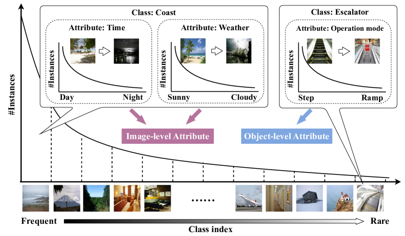
Figure 1: Inter-class long-tailed distribution and attribute-wise long-tailed distribution.

In Fig. 1, it is evident that there is a class-wise imbalance among different categories, especially for the head class such as “Coast”, which has a much larger number of samples than the tail class such as “Escalator”. Apart from class-wise imbalance, there is a significant difference in the number of samples corresponding to different attributes within a category (termed as attribute-wise imbalance for short). For example, in the category “Coast”, the number of samples during the day is much greater than that at night, and the number of samples on sunny days is also much greater than that on cloudy days. Even in the tail category “Escalator”, the number of samples in “Step Escalator” is greater than that in “Ramp Escalator”.

Attribute-wise imbalance is fundamentally more difficult to handle than class-wise imbalance, as shown in Fig. 2.

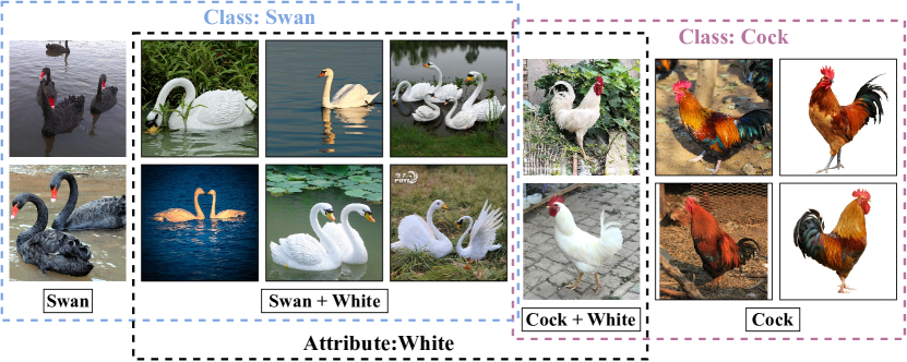
Figure 2: Spurious correlation of the “White” attribute with the “Swan” category. Firstly, black swans are more likely to be misclassified than white swans in the category “Swan”, even though they both belong to the same category. Secondly, the attribute “White” may be falsely correlated with “Swan”, so when “White” appears in images of “Cock”, there is a high risk that the “cock” will be misclassified as a “Swan”.

Current research mostly focuses on solving the class-wise long-tailed problem, where resampling [10, 11] or loss reweighting [12, 13] methods are often used to rebalance the training process. However, most of these methods sacrifice the performance of the head class to improve the performance of the tail class, which is like playing a performance seesaw, making it difficult to fundamentally improve the performance for all classes. Apart from resampling and reweighting, there are some methods (e.g., [14, 15]) believe that data imbalance does not affect feature learning, so the training of the model is divided into two stages of feature learning and classifier learning. However, this adjustment is only a trade-off between accuracy and precision [9, 16], and the confusion areas of similar attributes in the feature space learned by the model do not change. As depicted in Fig 2, it is the attribute-wise imbalance that leads to spurious correlations between the head attributes and a particular category. This means that these head attributes correspond to the spurious features (i.e., a confusing region in the feature space) of the category.

To alleviate the performance-degrading affects from spurious features, Arjovsky et. al proposed the concept of IRM [17], for which the construction of different environments is a prerequisite for training. The challenge in this paper is to construct controllable environments with different attribute distributions. Environments with different category distributions are easy to construct because the labels are explicit, while the attributes are implicit for most datasets. Therefore, even if the class-wise imbalance is completely eliminated, attribute-wise imbalance still exists. At the same time, because of the nature that attributes can be continuously superimposed and combined, the boundaries of attributes are also complex, thus we design a sampling method based on unsupervised learning. The result of this unsupervised learning portrays the distribution of attributes within the same category and can control the granularity of the portraying of attributes according to the setting of hyperparameters.

Our motivation is based on a reasonable assumption that the differences between samples within the same category are the result of the gradual separation and evolution of attributes. This is observed in a leading tree ( Fig. 3) in our previous work [18], where the gap from the root node to the leaf nodes doesn’t happen all at once, but is the result of continuous evolution and branching. The evolution is not only reflected at a Coarse-Grained level, but also within the same category where the transitions are more subtle. Within the same category of ‘2’, the samples along each path evolve gradually. We can recognize the implicit attributes of “upward tail” and “circle” with human perception, although it is not explicitly described by the algorithm. Without gaining knowledge on the attribute-wise distribution with the same class, the existing GLT method uses the try-and-error methodology to find poorly predicted environments and train invariant features across them [9]. In contrast, our method first find the samples that follow implicit attribute-wise evolution via unsupervised learning within each given class and construct effective environments.

Figure 3: A leading tree constructed from digit ‘2’ in MNIST dataset (taken from our previous work [18]), in which each path can reflect an implicit attribute within the same class. Note that this figure is used only to explain our intuition and motivation, we did not evaluate our method on MNIST dataset.

This paper proposes a framework termed as Cognisance, which is founded on Coarse-grained Leading Forest and Multi-center Loss. Cognisance handles class-wise and attribute-wise imbalance problems simultaneously by constructing different environments , in which we design a new sampling method based on a structure of samples called Coarse-Grained Leading Forest (CLF). A CLF is constructed by unsupervised learning that characterizes the attribute distributions within a class and guides the data sampling in different environments during training process. In the experimental setup of this paper, two environments are constructed, one of which is the original environment without special treatment, and the distributions of categories and attributes in the other are balanced. In order to gradually eliminate confusing pseudo-features during the training process, we design a new metric learning loss, Multi-Center Loss (MCL), which is inspired by [9] and [19], extends the center loss to its Invariant Risk Minimization (IRM) version. MCL enables our model to better learn invariant features and further improves the robustness when compared to its counterparts in [9] and [19]. In addition, the proposed framework is not coupled with a specific backbone model or loss function, and can be seamlessly integrated into other LT methods for performance enhancement.

Our contributions can be summarized as follows:

• We designed a novel unsupervised learning-based sampling scheme based on CLF to guide the sampling of different environments in the IRM process. This scheme deals with class-wise and attribute-wise imbalance simultaneously.

• We combined the idea of invariant feature learning and the property of CLF structure to design a new metric learning loss (MCL), which can enable the model to gradually remove the influence of pseudo-features during the training process. MCL improves the robustness of the model and takes into account both precision and accuracy of the prediction.

• We conducted extensive experiments on two existing benchmarks, ImageNet-GLT and MSCOCO-GLT, to demonstrate the effectiveness of our framework on further improving the performance of popular LT lineups against [9].

The remainder of the paper is structured as follows. Section II briefly introduces the closely related preliminaries. Section III gives detailed description of Cognisance framework. The experimental study is presented in Section IV and some discussion on the conceptualization and implementation of Cognisance are given in Section V. Finally, we reach the conclusion in Section VI.

II Related Work

II-A Long-Tailed Classification

The key challenge of long-tailed classification is to effectively deal with the imbalance of data distribution to ensure that excellent classification performance can be achieved both between the head and the tail. Current treatments for long-tailed classification can be broadly categorized into three groups [1]: 1) Class Re-balancing, which is the mainstream paradigm in long-tailed learning, aims to enhance the influence of tail samples on the model by means of re-sampling [20, 11, 21, 22], re-weighting [23, 24, 25, 26, 27] or logit adjustment [28] during the model training process, and some of these methods [14, 15] consider that the unbalanced samples do not affect the learning of the features, and thus divide feature learning and classifier learning into two phases, and perform operations such as resampling only in the classifier learning phase. 2) Information Augmentation based approaches seek to introduce additional information in model training in order to improve model performance in long-tailed learning. There are two approaches in this method type: migration learning [29, 30, 31] and data augmentation [32, 33, 34]. 3) Module Improvement seeks to improve network modules in long-tailed learning such as RIDE [35] and TADE [36], both of which deal with long-tail recognition independent of test distribution by introducing integrated learning of multi-expert models in the network.

In addition, a recent study proposed the concept of Generalized Long-Tailed Classification (GLT) [9], which first recognized the problem of long-tailed of attributes within a class and pointed out that the traditional long-tailed classification methods represent the classification model as $p(Y|X)$. This can be further decomposed as $p(Y|X)\propto p(X|Y)\cdot p(Y)$, the formula identifies the cause of class bias as $p(Y)$. However, the distribution of $p(X|Y)$ also changes in different domains, so the classification model is extended to the form of Eq. (1) based on the Bayesian Theorem in this study.

$$p(Y=k|z_{c},z_{a})=\frac{p(z_{c}|Y=k)}{p(z_{c})}\cdot\underbrace{\frac{p(z_{a}|Y=k,z_{c})}{p(z_{a}|z_{c})}}_{attribute\ bias}\cdot\underbrace{p(Y=k)}_{class\ bias},$$ (1)

where $z_{c}$ is the invariant present in the category, and the attribute-related variable $z_{a}$ is the domain-specific knowledge in different distributions. Taking the mentioned “swan” as an example, the attribute “color” of “Swan” belongs to $z_{a}$, while the attributes of “Swan” such as feathers and shape belong to $z_{c}$.

Remark: In practical applications, the formula does not impose the untangling assumption, i.e., it does not assume that a perfect feature vector $z=[z_{c};z_{a}]$ can be obtained, where $z_{a}$ and $z_{c}$ are separated.

II-B Invariant Risk Minimization

The main goal of IRM [17] is to build robust learning models that can have the same performance on different data distributions. In machine learning, we usually hope that the trained model can perform well on unseen data, which is called risk minimization. However, in practice, there may be distributional differences between the training data and the test data, known as domain shift, which causes the model to perform poorly on new domains. The core idea of IRM is to solve the domain adaptation problem by encouraging models to learn features that are invariant across data domains. This means that the model should focus on those shared features that are present in all data domains rather than overfitting a particular data distribution. The objective of IRM is shown in (2).

$$\begin{split}&\mathop{\min}\limits_{\begin{subarray}{c}\Phi:\mathcal{X}\rightarrow\mathcal{H}\\ w:\mathcal{H}\rightarrow\mathcal{Y}\end{subarray}}\sum\limits_{e\in\mathcal{E}_{tr}}R^{e}(w\circ\Phi)\\ s.t.\quad&w\in\mathop{\arg\min}\limits_{\overline{w}:\mathcal{H}\rightarrow\mathcal{Y}}R^{e}(\overline{w}\circ\Phi),\ for\ all\ e\in\mathcal{E}_{tr},\end{split}$$ (2)

where $\mathcal{E}_{tr}$ represents all training environments, $\mathcal{X}$, $\mathcal{H}$, and $\mathcal{Y}$ represent inputs, feature representations, and prediction results, respectively. $\Phi$ and $w$ are feature learner and classifier, respectively, and $R^{e}$ denotes the risk under the environment $e$, the goal of IRM is to find a general feature learning solution that can perform stably on all environments, thus improving the model’s generalization ability.

II-C Optimal Leading Forest

The CLF proposed in this paper starts with OLeaF [37], so we provide a brief introduction to its ideas and algorithms here. The concept of optimal leading forest originates from a clustering method based on density peak [38], and the two most critical factors in the construction of OLeaF are the density of a data point and the distance of the data point to its nearest neighbor with higher densitiy. Let ${\boldsymbol{I}}=\left\{1,2,...,N\right\}$ be the index set of dataset $\mathcal{X}$, and $d_{i,j}$ represent the distance between data points $\boldsymbol{x}_{i}$ and $\boldsymbol{x}_{j}$ (any distance metric can be used), and let $\rho_{i}=\sum_{j\in\boldsymbol{I}\backslash\{i\}}\exp\big{(}-(d_{i,j}/d_{c})^{2}\big{)}$ be the density of data point $\boldsymbol{x}_{i}$, where $d_{c}$ is the bandwidth parameter. If there exists $\xi_{i}=\arg\min_{j}\left\{d_{i,j}|\rho_{j}>\rho_{i}\right\}$, then a tree structure (termed as leading tree) can be established based on $\boldsymbol{\xi}=\{\xi_{i}\}_{i=1}^{N}$. Let $\delta_{i}=d_{\xi_{i},i}$, $\gamma_{i}=\rho_{i}\times\delta_{i}$, then the larger $\gamma_{i}$ represents the higher potential of the data point $\boldsymbol{x}_{i}$ to be selected as a cluster center. Intuitively, if an object $\boldsymbol{x}_{i}$ a has a large $\rho_{i}$, it means it has a lot of close neighbors; and if $\delta_{i}$ is large, it is far away from another data point with a larger $\rho$ value, so $\boldsymbol{x}_{i}$ has a good chance to become the center of a cluster. The root nodes (centers of clustering) can be selected based on the ordering of $\{\gamma_{i}\}$. In this way, an entire leading tree will be partitioned using the centers indicated by largest elements in $\{\gamma_{i}\}$, and the resultant collection of leading trees is called an Optimal Leading Forest (OLeaF).

The OLeaF structure has been observed has the capability of revealing the attribute-wise difference evolution [18], so it can be employed to construct the environments in GLT training. Although the unsupervised learning procedure dose not automatically tag the attribute label of each path, but we could recognize via human cognitive ability the meaningfulness of each path (e.g., the “circle” attribute and “upward tail” attribute in Fig. ).

III Cognisance framework

In order to improve the generalization ability of the model on data with different category distributions and different attribute distributions, this paper proposes an framework named Cognisance based on invariant feature learning, which firstly uses Coarse-Grained Leading Forest to construct different environments considering both class-wise and attribute-wise imbalances. With a newly designed Multi-Center Loss, the model is allowed to learn invariant features in each data domain instead of overfitting a certain distribution to solve the multi-domain adaptation problem.

III-A Coarse-Grained Leading Forest

We designed a new clustering algorithm Coarse-Grained Leading Forest in combination with the construction of OLeaF [18], and its construction process is shown in Algorithm 1.

1) Compute the distance matrix between the sample points in the dataset X using an arbitrary distance metric. Then compute the density of sample point $i$ is computed as in Eq. (3):

$$\rho_{i}=\sum_{j\in\boldsymbol{I}\backslash\{i\}\backslash\textbf{O}_{i}}\exp\big{(}-(d_{i,j}/d_{rd})^{2}\big{)},$$ (3)

where $\boldsymbol{I}=\left\{1,2,...,N\right\}$ is the index set of dataset $\boldsymbol{X}$, $d_{rd}$ is the radius of the hypersphere for computing density centered at $\boldsymbol{x}_{i}$, $\boldsymbol{O}_{i}$ is the set of samples lie outside of the hypersphere that do not contribute to $\rho_{i}$.

2) Sort the samples in descending order according to the density value, denoted as $\boldsymbol{S}$ the indices of the sorted data, i.e., $\boldsymbol{S}_{i}$ is the index of the data point with the $i$-th largest density value.

3) Form Coarse-Grained node on the points in $\boldsymbol{S}$ sequentially, which relies on the hyperparameter $d_{rn}$. If the data point $\boldsymbol{S}_{i}$ has not yet been merged into a Coarse-Grained node, then the data point $\boldsymbol{S}_{i}$ and the points within $d_{rn}$ distance from it are formed into a Coarse-Grained node, i.e.:

$$\boldsymbol{C}(i)=\{\boldsymbol{S}_{i}\}\cup\boldsymbol{K}(i)\ \backslash\ \boldsymbol{A},\quad\boldsymbol{S}_{i}\notin\boldsymbol{A},$$ (4)

where $\boldsymbol{C}(i)$ are members of the newly generated Coarse-Grained node, $\boldsymbol{S}_{i}$ will be a prototype for that Coarse-Grained node, $\boldsymbol{K}(i)$ is the set of nodes that are within $d_{rn}$ from $\boldsymbol{S}_{i}$, i.e., $\boldsymbol{K}(i)=\{j\ |\ j\in\boldsymbol{I},\ d_{S_{i},j}<d_{rn}\}$, and $\boldsymbol{A}$ is the set of visited nodes, i.e., the set of nodes that have already been merged into a particular Coarse-Grained node. Note that if $\boldsymbol{S}_{i}$ itself is already in $\boldsymbol{A}$ then it skips the creation of Coarse-Grained node and continues to process the next node in $\boldsymbol{S}$.

Input: All training samples of a given category $\textbf{{X}}_{c}$.

Output: A Coarse-Grained Leading Forest clf for a given category.

Parameter : $d_{rd}$ as the hypersphere radius to compute density, $d_{rn}$ as the radius of the Coarse-Grained node.

1

2$N$ = number of samples in $\textbf{{X}}_{c}$;

3 dist = calculate_distance($\textbf{{X}}_{c}$);

4 density = calculate_density(dist, $d_{rd}$);

5 $\boldsymbol{S}$ = argsort(density, descend=T);

// Record the index of accessed samples

6 $\boldsymbol{A}$ = initial_vector($N$, F);

7

8for $idx$ in range($N$) do

9       i = $\boldsymbol{S}[idx]$;

10       if $\boldsymbol{A}$[i]==T then

11             continue;

12            

13       end if

      // Combine unvisited points within $d_{rn}$

14       $\boldsymbol{C}(i)$ = $\{i\}\bigcup\{j|\boldsymbol{A}[j]==$F$\;\&\&\;\textit{dist}[\textit{i,j}]\leq d_{rn})\}$;

15       $\boldsymbol{A}[j]$= T for $j\in\boldsymbol{C}(i)$;

16       $l_{i}$ = find_leader($i$, $d_{rn}$);

       // $\boldsymbol{C}(i)$ becomes a root if no $l_{i}$ exists

17       if $l_{i}\neq$ null then

18             $\boldsymbol{C}(i)$.leader = $\boldsymbol{C}(l_{i})$;

19            

20       end if

21      else

22             clf.root.append($\boldsymbol{C}(i)$);

23            

24       end if

25      

26 end for

27

28return clf;

Algorithm 1 Construction of CLF

4) Find the leading node of the newly constructed Coarse-Grained node. Here, the problem is transformed into finding the leading node of the prototype $\boldsymbol{S}_{i}$ of a Coarse-Grained node, denoted as $l_{i}$, and then $\boldsymbol{C}(l_{i})$ is assigned as the leading node of $\boldsymbol{C}(i)$. The process of finding the leading node $\boldsymbol{C}(l_{i})$ of $\boldsymbol{C}(i)$ can be formulated as Eq. (5):

$$l_{i}=\arg\min_{j}\left\{d_{S_{i},j}|\rho_{j}>\rho_{S_{i}}\right\},j\in{\boldsymbol{I}\backslash\{\boldsymbol{S}_{i}}\}\backslash\boldsymbol{O}_{S_{i}},$$ (5)

where $\boldsymbol{O}_{S_{i}}$ is the set of nodes whose distance from $\boldsymbol{S}_{i}$ exceeds $d_{rd}$. Note that $l_{i}$ may not exist, and when $l_{i}$ is not found, the Coarse-Grained node $\boldsymbol{C}(i)$ is the root of a leading tree in the whole Coarse-Grained leading forest. Also, since the density of nodes in $\boldsymbol{S}$ is decreasing, when $l_{i}$ is found, it must have been processed and already merged into $\boldsymbol{C}(i)$ since $l_{i}$ is denser.

III-B Sampling based on CLF

By constructing the CLF we can portray the attribute distributions within a category, and by adjusting the hyperparameters $d_{rn}$ and $d_{rd}$, we can control the granularity of the distributions portraying. An exemplar CLF in an environment of different attribute distributions is shown in Fig. 4. One can categorize all the data points on each path from root to a leaf node as members of a certain attribute, because each path represents a new direction of attribute evolution.

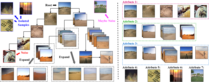
Figure 4: The left is an example of CLF constructed for category “sand”, while the right is an example of attribute splitting using CLF. Each path from the root to the leaf node can be considered as an (implicit) attribute, and the samples within the Coarse-Grained nodes are very similar that require an appropriate reduction in sampling weights. In addition, the samples within the red and pink boxes demonstrate the potential of CLF for noisy recognition.

After the samples of each attribute is determined, we can refer to the idea of class-wise resampling [14] to resample on the attributes (compute the probability of each sampled objects from class $j$ ), as shown in (6).

$$p_{j}=\frac{(n_{j})^{q}}{\sum_{i=1}^{C}(n_{i})^{q}},$$ (6)

where $j$ represents the class index, $n_{j}$ is the number of samples of class $j$, and $C$ the total number of classes. $q\in[0,1]$ is a user-defined parameter, and class-wise balanced sampling is performed when $q=0$.

As shown in Algorithm 2, when sampling different attributes within a category, the idea is the same as class-wise sampling. When applying Eq. (6), the only difference is to regard $j$ as the attribute index, $n_{j}$ as the number of samples of attribute $j$, and $C$ as the total number of attributes. Besides, it should be noted that the same sample may belongs to more than one attribute collection (e.g., the root node appears in all branches of the same tree, so it has all the attributes under consideration), so the weight of such a sample needs to be penalized. At the same time, due to the concept of Coarse-Grained node in our algorithm, as shown in Fig. 4, the members in the Coarse-Grained nodes are highly alike, so the sampling weight of the members in the Coarse-Grained nodes should be reduced accordingly. In this paper, we let the members of a coarse node $\boldsymbol{C}(i)$ equally share the weight of $\boldsymbol{C}(i)$.

Input: A Coarse-Grained Leading Forest clf, balance factor q

Output: The sampling probability of each sample within a certain category weights

1 weights = initial_vector(default=0, size=$|$clf$|$);

2 paths = generate_path(clf);

3 repetitions = get_repetition(paths);

4 path_weight = get_path_weight(paths, q) using Eq. (6);

5 foreach path in paths do

6      

7      node_weight = path_weight / $\text{len}(\textit{path})$;

       // All nodes are considered coarse

8       foreach node in path do

9             node_weight /= $\text{len}(\textit{node.members})$;

10            

11       end foreach

12      

13 end foreach

14weights $/=\textit{repetitions}$;

15 return weights;

Algorithm 2 Attribute-wise sampling via CLF

We provide a detailed description on attribute balanced sampling based on the CLF in Fig. 4 (ignoring isolated samples for demonstration purposes). Firstly, each path from root to a leaf node reflects the evolution along an attribute, which means that if you want to evenly sample the data of each attribute, you only need to assign equal sampling weights to the collection of data in each path. Where for nodes that are repeated in multiple paths, we simply divide their sampling weight by the number of repetitions as a penalty. Take the example of calculating the weight of the root node, firstly since there are three attribute groups, so $weight=\frac{1}{3}$, and then the node’s weight in the three attribute groups are $\frac{1}{5}$, $\frac{1}{4}$, and $\frac{1}{5}$, so the root node’s sampling weights globally are $\frac{1}{15}$, $\frac{1}{12}$, and $\frac{1}{15}$, and summing up the three weights yields $weight=\frac{13}{60}$, and finally an appropriate penalty is to be applied, i.e., $weight=\frac{weight}{repetition}=\frac{13}{180}$. Furthermore, for a CoarseNode containing multiple samples, the penalty is similar, setting the sampling weight of each sample to $weight=CoarseNode.weight/CoarseNode.length$. Taking the second Coarse-Grained node in Attribute 2 as an example, the sampling weight of this node is $weight=(\frac{1}{3}\times\frac{1}{4}+\frac{1}{3}\times\frac{1}{5})/2=\frac{3}{40}$, and the sampling weight of each sample in this Coarse-Grained node is $weight=\frac{3/40}{2}=\frac{3}{80}$.

III-C Multi-Center Loss

Multiple training environments for invariant feature learning were constructed in the previous step, and the next might be training the model with the objective function of IRM [17]. However, since the original IRM loss does not converge occasionally in experiments, we designed a new goal Multi-Center Loss based on the idea of IRM and the center loss in IFL [9], which can be formulated as:

$$\begin{split}&\mathop{\min}\limits_{\theta,\ w}\sum\limits_{e\in\mathcal{E}}\sum\limits_{i\in e}L_{cls}\big{(}f(x_{i}^{e};\ \theta),\ y_{i}^{e};\ w\big{)}\\ \mathrm{s.t.}&\quad\theta\in\mathop{\arg\min}\limits_{\Theta}\sum\limits_{e\in\mathcal{E}}\sum\limits_{i\in e}{\|f(x_{i}^{e};\ \Theta)-\mathcal{C}(x_{i})\|}_{2},\end{split}$$ (7)

where $\Theta$ and $w$ are the learnable parameters of the backbone and classifier, respectively, $x_{i}^{e}$ and $y_{i}^{e}$ are the $i$-th instance in environment $e$ and its label, respectively, $\mathcal{E}$ is all the training environments, $f(x_{i}^{e};\ \theta)$ is the feature extracted by the backbone from $x_{i}^{e}$, $L_{cls}\big{(}f(x_{i}^{e};\ \theta),\ y_{i}^{e};\ w\big{)}$ is the classification loss under environment $e$ (with arbitrary loss function), and $\mathcal{C}(x_{i})$ is the learned feature of the center to which $x_{i}^{e}$ belongs (in all environments $\mathcal{E}$). Note that the number of centers in each category $n_{c_{y_{i}}}\geq 1$, and the center of $x_{i}^{e}$ depends on which tree in the CLF contains $x_{i}^{e}$, i.e., $n_{c_{y_{i}}}\equiv n_{t_{y_{i}}}$, where $n_{t_{y_{i}}}$ is the number of trees in the CLF constructed from all samples of that category, and the initial value of $\mathcal{C}(x_{i})$ is the value of the prototype (the root) of the tree containing $x_{i}^{e}$. The practical version of this optimization problem is shown in Eq. 8, where $L_{IFL}={\|f(x_{i}^{e};\ \theta)-\mathcal{C}(x_{i})\|}_{2}$ is the constraint loss for invariant feature learning and $\alpha>0$ is a trade-off parameter:

$$\begin{split}\mathop{\min}\limits_{\theta,\ w}\sum\limits_{e\in\mathcal{E}}\sum\limits_{i\in e}L_{mc}&=\mathop{\min}\limits_{\theta,\ w}\sum\limits_{e\in\mathcal{E}}\sum\limits_{i\in e}L_{cls}+\alpha\cdot L_{IFL}\\ &=\mathop{\min}\limits_{\theta,\ w}\sum\limits_{e\in\mathcal{E}}\sum\limits_{i\in e}L_{cls}\big{(}f(x_{i}^{e};\ \theta),\ y_{i}^{e};\ w\big{)}\\ &\quad\ +\alpha\cdot{\|f(x_{i}^{e};\ \theta)-\mathcal{C}(x_{i})\|}_{2}.\end{split}$$ (8)

This loss is the IRM version of center loss that improves the robustness over the original version of center loss. As in the previous introduction of CLF, for some artificial datasets, even within the same category there may be great the difference between samples, i.e., the number of trees in CLF is greater than one, as shown in Fig. 5. The category “garage” can actually be divided into three categories: “Outside the garage”, “Inside the garage with car”, and “Inside the garage without car”. The features of these three subcategories vary greatly. Using only one center would make each category’s features gradually approach one center during the training process, which will actually degrade the quality of learned features. This is the exact motivation for proposing Multi-Center Loss.

Figure 5: Multiple trees in the CLF of category “garage” (only part of it is shown), there are multiple subclasses in the category “garage”, e.g., outside the garage, inside the garage (parked cars), and inside the garage (no parked cars), and there is a huge disparity among these subclasses.

III-D Cognisance Framework

The overall framework of Cognisance is shown in Fig. 6. Each environment is sampled according to a pair of parameter $(q_{cls},q_{attr})$, with $(q_{cls}$ being the balance factor for class-wise sampling and $(q_{attr}$ being the balance factor for attribute-wise sampling. The model parameters can be shared for training under the constraint of MCL. The paths to portray the implicit attribute distribution during sampling is achieved through CLF, while the number of centers in MCL is determined by the number of trees in CLF of the corresponding category.

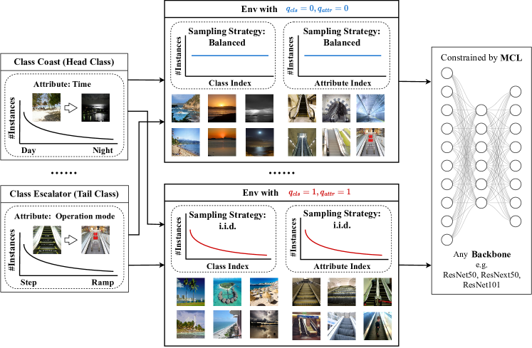
Figure 6: Overall framework diagram. Different environments have different sampling strategies, where $q_{cls}$ and $q_{attr}$ are balancing factors for class-wise sampling and attribute-wise sampling, respectively.

The algorithmic description of Cognisance is shown in Algorithm 3, which consists of two stages:
1) Since the initial features of the samples need to be used for clustering when constructing CLF, $M$-round normal sampling training is required to obtain an initial model with imperfect predictions;
2) The initial features are used to construct the CLF, and different environments are constructed through the CLF and different balance factor pairs. For example, in the experimental phase, this article sets up two environments with balance factor pairs of $(q_{cls}^{e_{2}}=0,q_{attr}^{e_{2}}=0)$ and $(q_{cls}^{e_{1}}=1,q_{attr}^{e_{1}}=1)$, where the former is a balanced sampling environment for both categories and attributes and the latter is a normal i.i.d. sampling environment that exhibits both class-wise and attribute-wise imbalance. Then, the feature learner is continuously updated and the centers in the CLF and MCL are updated accordingly. The number of epoch steps for executing updates in the second stage can be adjusted, rather than being fixed to one update per epoch.

Input: An original training set $\{(x,y)\}$; balance parameter pairs $\{(q_{cls}^{e},q_{attr}^{e})\}$ for different environments.

Output: backbone $f(\cdot;\theta)$, classifier $g(\cdot;w)$

1 Initialize: backbone $f(\cdot;\theta)$, classifier $g(\cdot;w)$;

2 for $M$ warm-up epochs do

       // Optimize the model for any loss

3       $\theta,w\leftarrow\hat{\theta},\hat{w}\in\text{arg min}_{\theta,w}L_{cls}(g(f(x;\theta);w),y)$;

4      

5 end for

6$clf=\text{ClfConstruct}(\{(x,y)\},\theta)$ (Alg. 1);

7 $\mathcal{E}=\text{EnvConstruct}(\{(q_{cls}^{e},q_{attr}^{e})\},clf)$ (Alg. 2);

8 for $N$ epochs do

9       $\{(x^{e},y^{e})\}=\text{DataLoader}(\mathcal{E})$;

10       $\{C_{y}\}=\text{ReadCenters}(clf)$;

11       $\theta,w\leftarrow\hat{\theta},\hat{w}\in\text{arg min}_{\theta,w}L_{cls}(g(f(x;\theta);w),y)+\alpha\cdot L_{IFL}(f(x;\theta),\{C_{y}\})$;

12       $clf=\text{ClfConstruct}(\{(x,y)\},\theta)$;

13       $\mathcal{E}=\text{EnvConstruct}(\{(q_{cls}^{e},q_{attr}^{e})\},clf)$;

14      

15 end for

16return backbone $f(\cdot;\theta)$, classifier $g(\cdot;w)$;

Algorithm 3 Cognisance framework

IV Experiment

TABLE I: Evaluation of CLT and GLT protocols on ImageNet-GLT. Among 48 comparisons against the competing models, the family of ?+Cognisance won for 43 times.

Protocols   width 1pt		Class-Wise Long Tail (CLT) Protocol   width 1pt				Generalized Long Tail (GLT) Protocol
$\langle$Accuracy $|$ Precision$\rangle$   width 1pt		$Many_{C}$	$Medium_{C}$	$Few_{C}$	Overall   width 1pt	$Many_{C}$	$Medium_{C}$	$Few_{C}$	Overall
Re-balance	Baseline   width 1pt	$58.39|38.35$	$36|52.15$	$13.98|55.34$	$41.65|47.11$   width 1pt	$50.7|32.5$	$27.8|43.99$	$10.18|47.7$	$34.32|39.95$
	BBN   width 1pt	$62.66|43.45$	$44.36|55.44$	$14.66|57.57$	$47.22|50.96$   width 1pt	$53.37|36.45$	$34.97|46.81$	$10.73|46.08$	$38.7|42.56$
	BLSoftmax   width 1pt	$54.03|47.07$	$41.65|46.83$	$28.37|37.58$	$44.61|45.54$   width 1pt	$46.45|40.45$	$32.67|38.59$	$21.38|29.57$	$36.49|37.98$
	Logit-Adj   width 1pt	$53.3|49.05$	$43.49|44.12$	$31.86|35$	$45.67|44.72$   width 1pt	$45.43|41.75$	$34.2|35.9$	$24.58|27.78$	$37.25|37.02$
	GLTv1   width 1pt	$62.51|42.32$	$38.69|57.23$	$17.41|\textbf{65}$	$45.03|52.43$   width 1pt	$54.4|36.23$	$30.18|49.61$	$12.64|55.47$	$37.24|45.14$
2-10[0.8pt/3pt]	* Baseline + Cognisance   width 1pt	$\textbf{62.84}|42.82$	$39.62|57.25$	$18.61|61.55$	$45.76|52.12$   width 1pt	$\textbf{54.53}|36.47$	$31.3|49.99$	$13.8|\textbf{58.27}$	$37.97|45.82$
	* BLSoftmax + Cognisance   width 1pt	$58.37|53.88$	$\textbf{44.98}|51.97$	$33.82|39.05$	$\textbf{48.66}|50.8$   width 1pt	$49.92|46.89$	$\textbf{36.11}|44.31$	$26.14|30.03$	$\textbf{40.14}|43.2$
	* Logit-Adj + Cognisance   width 1pt	$43.3|\textbf{75.13}$	$41.19|\textbf{59.08}$	$\textbf{45.43}|27.11$	$42.92|\textbf{60.7}$   width 1pt	$36.01|\textbf{70.18}$	$32.6|\textbf{52.48}$	$\textbf{36.26}|21.76$	$34.51|\textbf{54.95}$
Augment	Mixup   width 1pt	$60.14|38.02$	$31.46|56.67$	$7.59|32.82$	$39.35|45.63$   width 1pt	$51.68|32.21$	$23.87|48.25$	$5.47|28.27$	$32.23|38.84$
	RandAug   width 1pt	$64.14|42.23$	$40.1|58.27$	$14.96|59.51$	$45.94|52.04$   width 1pt	$55.7|35.87$	$31.61|50.15$	$10.2|47.29$	$38.03|44.01$
2-10[0.8pt/3pt]	* Mixup + Cognisance   width 1pt	$67.86|47.9$	$45.5|62.76$	$24.98|\textbf{67.56}$	$51.37|57.54$   width 1pt	$59.28|40.95$	$36.16|54.09$	$17.63|57.72$	$42.63|49.38$
	* RandAug + Cognisance   width 1pt	$\textbf{69.12}|\textbf{49.31}$	$\textbf{47.64}|\textbf{63.08}$	$\textbf{26.97}|67.01$	$\textbf{53.13}|\textbf{58.16}$   width 1pt	$\textbf{60.85}|\textbf{42.3}$	$\textbf{38.46}|\textbf{55.21}$	$\textbf{19.9}|\textbf{60.11}$	$\textbf{44.63}|\textbf{50.78}$
Ensemble	TADE   width 1pt	$57.3|\textbf{55.22}$	$46.85|50.29$	$\textbf{34.69}|37.93$	$49.21|50.41$   width 1pt	$49.61|\textbf{48.19}$	$37.55|42.59$	$\textbf{27.52}|32.21$	$40.87|43.28$
	RIDE   width 1pt	$63.18|51.44$	$47.67|52.55$	$29.91|47.38$	$51.21|51.33$   width 1pt	$54.83|44.02$	$38.25|44.2$	$22.77|38.12$	$42.56|43.21$
2-10[0.8pt/3pt]	* TADE + Cognisance   width 1pt	$60.69|55.15$	$48.15|52.22$	$33.38|42.12$	$50.95|51.88$   width 1pt	$52.77|48.15$	$39.09|44.06$	$26.51|33.32$	$42.68|44.08$
	* RIDE + Cognisance   width 1pt	$\textbf{64.83}|54.6$	$\textbf{50.95}|\textbf{56.21}$	$33.28|\textbf{50.15}$	$\textbf{53.85}|\textbf{54.66}$   width 1pt	$\textbf{57.1}|47.63$	$\textbf{42}|\textbf{48.42}$	$25.5|\textbf{41.23}$	$\textbf{45.57}|{47.03}$

TABLE II: Evaluation of CLT and GLT protocols on MSCOCO-GLT. Among 48 comparisons against the competing models, the family of ?+Cognisance won for 44 times.

Protocols   width 1pt		Class-Wise Long Tail (CLT) Protocol   width 1pt				Generalized Long Tail (GLT) Protocol
$\langle$Accuracy $|$ Precision$\rangle$   width 1pt		$Many_{C}$	$Medium_{C}$	$Few_{C}$	Overall   width 1pt	$Many_{C}$	$Medium_{C}$	$Few_{C}$	Overall
Re-balance	Baseline   width 1pt	$81.27|71.08$	$74.13|76.06$	$50.17|85.61$	$71.88|76.15$   width 1pt	$74.59|64.82$	$66.25|69.08$	$35.75|77.22$	$63.1|69.14$
	BBN   width 1pt	$83.59|70.21$	$76.13|76.3$	$47.25|\textbf{90.98}$	$72.98|77.02$   width 1pt	$75.36|61.97$	$68.29|68.61$	$31.75|\textbf{81.38}$	$63.41|68.73$
	BLSoftmax   width 1pt	$80.77|71.87$	$75.67|69.94$	$45.25|90.08$	$71.31|74.84$   width 1pt	$73.23|65.13$	$68.63|62.64$	$32.08|79.6$	$62.81|67.09$
	Logit-Adj   width 1pt	$81.55|73.95$	$76|75.55$	$\textbf{60.83}|82.04$	$74.97|76.28$   width 1pt	$73.64|66.98$	$68.71|67.61$	$\textbf{46.58}|70.69$	$66|68.01$
	GLTv1   width 1pt	$82.45|73.09$	$76.42|79.53$	$55.58|86.87$	$74.4|78.6$   width 1pt	$76.41|67.07$	$67.33|70.54$	$39.75|81.02$	$65.07|71.39$
2-10[0.8pt/3pt]	* Baseline + Cognisance   width 1pt	$\textbf{83}|73.95$	$77.88|\textbf{80.48}$	$55.92|90.08$	$75.28|\textbf{79.99}$   width 1pt	$\textbf{76.91}|68.24$	$67.5|\textbf{71.41}$	$39.67|80.33$	$65.31|\textbf{72.05}$
	* BLSoftmax + Cognisance   width 1pt	$83|74.17$	$78.37|76.24$	$53.92|86.51$	$75.07|77.58$   width 1pt	$75.86|67.98$	$70.46|68.14$	$40.08|80.26$	$66.22|70.59$
	* Logit-Adj + Cognisance   width 1pt	$82.68|\textbf{77.16}$	$\textbf{80.17}|75.45$	$59.17|83.54$	$\textbf{76.78}|77.77$   width 1pt	$75.14|\textbf{70.56}$	$\textbf{71.54}|66.34$	$45.83|73.9$	$\textbf{67.59}|69.5$
Augment	Mixup   width 1pt	$82.41|72.95$	$73.12|79.53$	$54.33|87.47$	$72.76|78.68$   width 1pt	$74.64|66.43$	$65.33|71$	$36|78.11$	$62.79|70.74$
	RandAug   width 1pt	$84.23|74.33$	$77.42|79.28$	$56.33|87.07$	$75.64|79.01$   width 1pt	$77.91|68.56$	$69.67|70.95$	$39.58|78.43$	$66.57|71.59$
2-10[0.8pt/3pt]	* Mixup + Cognisance   width 1pt	$85|76.96$	$81.42|83.19$	$\textbf{63.33}|88.89$	$79.03|82.01$   width 1pt	$79.23|\textbf{70.89}$	$72.25|\textbf{74.84}$	$\textbf{46.5}|80.62$	$\textbf{69.57}|\textbf{74.54}$
	* RandAug + Cognisance   width 1pt	$\textbf{86.55}|\textbf{78.31}$	$81.5|82.82$	$62.42|\textbf{90.29}$	$\textbf{79.47}|\textbf{82.65}$   width 1pt	$\textbf{79.05}|69.93$	$\textbf{72.92}|74.51$	$44.33|\textbf{81.82}$	$69.33|74.28$
Ensemble	TADE   width 1pt	$83.55|76.47$	$80.79|73.89$	$50.5|89.34$	$75.57|78.06$   width 1pt	$77.18|68.62$	$71.58|65.63$	$33.5|82.32$	$65.83|70.22$
	RIDE   width 1pt	$84.23|77.56$	$82.29|77.79$	$58.42|89.69$	$78.09|80.16$   width 1pt	$77.45|71.2$	$75.17|68.67$	$41.25|83.33$	$69.02|72.66$
2-10[0.8pt/3pt]	* TADE + Cognisance   width 1pt	$85.59|77.48$	$82.25|77.85$	$55.08|90.4$	$77.9|80.31$   width 1pt	$79|70.54$	$73.96|68.94$	$40.67|\textbf{83.65}$	$68.98|72.59$
	* RIDE + Cognisance   width 1pt	$\textbf{86.27}|\textbf{79.64}$	$\textbf{83.13}|\textbf{79.89}$	$\textbf{63.5}|\textbf{90.41}$	$\textbf{80.26}|\textbf{81.98}$   width 1pt	$\textbf{80.09}|\textbf{72.77}$	$\textbf{75.17}|\textbf{71.45}$	$\textbf{47.83}|83.03$	$\textbf{71.38}|\textbf{74.34}$

IV-A Evaluation Protocols

Before conducting the experiment, it is necessary to first introduce two new evaluation protocols: CLT Protocol and GLT Protocol, both of which were proposed in the first baseline of GLT [9]:

• Class wise Long Tail (CLT) Protocol: The samples in the training set follow a long-tailed distribution, which means that they are normally sampled from the LT dataset, while the samples in the test set are balanced by class. Note that the issue of attribute distribution is not considered in CLT, as the training and testing sets of CLT have the same attribute distribution and different class distributions, so the effectiveness of category long tail classification can be evaluated.

• Generalized Long Tail (GLT) Protocol: Compared with CLT protocol, the difference in attribute distribution is taken into account, that is, the attribute bias in Eq. (1) is introduced. The training set in GLT is the same as that in CLT and conforms to the LT distribution, while the attribute distribution in the test set tends to be balanced. Since attribute-wise imbalance is ubiquitous, the training set and test set in GLT have different attribute distributions and different class distributions. Therefore, it is reasonable to evaluate the model’s ability to handle both class-wise long-tailed and attribute-wise long-tailed classification with GLT protocol.

IV-B Datasets and Metrics

We evaluated Cognisance and compared it against the LT and GLT methods on two benchmarks, MSCOCO-GLT, and ImageNet-GLT, which are proposed in the first baseline of GLT [9].
ImageNet-GLT is a long-tailed subset of ImageNet [39], where the training set contains 113k samples of 1k classes, and the number of each class ranges from 570 to 4. The number of test set in both CLT and GLT protocols is 60k, and the test set are divided into three subsets according to the following class frequencies: #sample > 100 for $Many_{C}$, 100 $\geq$ #sample $\geq$ 20 for $Medium_{C}$, and #sample <20 for $Few_{C}$. Note that in constructing the test set for attribute balancing in this dataset, the images in each category were simply clustered into 6 groups using k-means, and then 10 images were sampled for each group in each category.

MSCOCO-GLT is a long-tailed subset of MSCOCO-Attribute [40], a dataset explicitly labeled with 196 different attributes, where each object with multiple labels is cropped as a separate image. The train set contains 144k samples from 29 classes, where the number of each class ranges from 61k to 0.3k, and the number of test set is 5.8k in both the CLT and GLT protocols, and the test set are divided into three subsets according to the following category frequencies: $Index_{C}$ $\leq$ 10 for $Many_{C}$ , 22 $\geq$ $Index_{C}$ $>$ 10 for $Medium_{C}$ and $Index_{C}$ > 22 for $Few_{C}$ , where $Index_{C}$ is the index of the category in ascending order.

Evaluation Metrics. In the experiments of this paper, three evaluation metrics are used to assess the performance of each methods: 1) Accuracy $\triangleq\frac{\sum_{i=1}^{N}{\rm TP}_{i}}{\sum_{i=1}^{N}({\rm TP}_{i}+{\rm FN}_{i})}$, which is also used in traditional long-tailed methods for the Top1-Accuracy or micro-averaged recall. In the above two formulas, $N$ denotes the total number of categories, and ${\rm TP}_{i}$, ${\rm FP}_{i}$, and ${\rm FN}_{i}$ denote the number of true positives, false positives, and false negatives in the $i$th category, respectively; 2) Precision $\triangleq\frac{1}{N}\sum_{i=1}^{N}\left(\frac{{\rm TP}_{i}}{{\rm TP}_{i}+{\rm FP}_{i}}\right)$; 3) the harmonic mean of accuracy and precision: $\text{F1-Score}^{*}\triangleq\frac{2\times(\text{Accuracy}\times\text{Precision})}{(\text{Accuracy}+\text{Precision})}$, the reason for introducing this metric is to better reveal the accuracy-precision trade-off problem [9] that has not been focused on in the traditional inter-class long-tailed methods.

IV-C Comparisons with LT Line-up

Cognisance handles both the class-wise long-tailed problem and the attribute-wise long-tailed problem by eliminating the false correlation caused by attributes, and can be seamlessly integrated with other LT methods. In the following comparison experiments, the backbone of the “Baseline” is resnext50, and its loss function is cross-entropy loss. For other methods, we follow the state-of-the-art long-tailed research [1] and [9] to classify current long-tailed methods into three categories: 1) Class Re-balancing, 2) Information Augmentation, and 3) Module Improvement. Two or three effective methods from each of these three categories are taken for comparison and enhancement, among which BBN [15], BLSoftmax [23] and Logit-Adj [7] are chosen for Class Re-balancing category, Mixup [34] and RandAug [32] for Information Augmentation, and RIDE [35] and TADE [36] for Module Improvement.

In addition, we have included the first strong baseline GLTv1 [9] in the GLT domain as a comparison. In Table I and Table II, the methods with an asterisk are the ones integrated with our component, and the bold-faced numbers are the optimal results in the category of the method. It is evident that Cognisance achieved promising results in all the classifications, especially when combined with the method RandAug or the method RIDE.

Cognisance is able to deal with both attribute-wise long-tailed and class-wise long-tailed, although the starting point of this method is to solve the problem of attribute long-tailed within the class. It meets the challenge of class-wise imbalance by eliminating the false correlation caused by long-tailed attributes [9]. Fig. 7 shows the improvements Cognisance achieved over the existing LT approaches w.r.t. the two sampling protocols (CLT and GLT) for the two benchmarks (ImageNet-GLT and COCO-GLT). One can see that the performance of all the methods has been degraded when sampling protocol is transferred from CLT to GLT, which demonstrates that the long-tailed problem is not purely class-wise but also attribute-wise (which is even more challenging). Cognisance can improve the performance of all existing popular LT methods on all protocols and benchmarks with an average increase up to 5%.

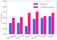
(a) CLT protocol, ImageNet-GLT

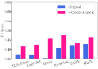
(b) GLT protocol, ImageNet-GLT

(c) CLT protocol, MSCOCO-GLT

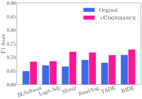
(d) GLT protocol, MSCOCO-GLT

Figure 7: Cognisance enhancements to existing LT methods

Finally, Table III records the experimental results of various methods on the test set of long-tailed distribution, which is consistent with the distribution of the training set. It can be seen that compared with other methods, our method achieves very encouraging results on all evaluation metrics.

TABLE III: Evaluation of ImageNet-GLT and MSCOCO-GLT on LT test set. Among 18 comparisons against the competing models, the family of ?+Cognisance won for 16 times.

Benchmarks   width 1pt		ImageNet-GLT   width 1pt			MSCOCO-GLT
Overall Evaluation   width 1pt		$Acc$	$Prec$	$F1$   width 1pt	$Acc$	$Prec$	$F1$
Re-balance	Baseline   width 1pt	53.93	44.46	48.74   width 1pt	85.74	79.98	82.76
	BBN   width 1pt	58.6	48.9	53.32   width 1pt	84.84	78.04	81.3
	BLSoftmax   width 1pt	51.73	41.97	46.34   width 1pt	83.69	73.81	78.44
	Logit-Adj   width 1pt	50.94	40.58	45.17   width 1pt	85.28	73.6	79.01
	GLTv1   width 1pt	58.28	50.43	54.07   width 1pt	86.67	81.88	84.21
2-8[0.8pt/3pt]	* Baseline + Cognisance   width 1pt	58.85	50.98	54.64   width 1pt	86.86	81.24	83.96
	* BLSoftmax + Cognisance   width 1pt	56.24	47.58	51.55   width 1pt	86.55	78.48	82.32
	* Logit-Adj + Cognisance   width 1pt	43.61	55.15	48.71   width 1pt	85.52	73.36	78.98
Augment	Mixup   width 1pt	55.25	46.76	50.66   width 1pt	86.95	82	84.4
	RandAug   width 1pt	59.88	51.28	55.25   width 1pt	87.64	81.02	84.2
2-8[0.8pt/3pt]	* Mixup + Cognisance   width 1pt	64.09	56.57	60.09   width 1pt	88.81	81.55	85.03
	* RandAug + Cognisance   width 1pt	65.15	56.85	60.72   width 1pt	89.12	84.02	86.49
Ensemble	TADE   width 1pt	55.21	46.52	50.49   width 1pt	86.57	79.91	83.1
	RIDE   width 1pt	60.17	48.28	53.58   width 1pt	88.03	81.79	84.8
2-8[0.8pt/3pt]	* TADE + Cognisance   width 1pt	58.06	47.44	52.21   width 1pt	88	81.72	84.74
	* RIDE + Cognisance   width 1pt	62.11	50.8	55.89   width 1pt	89.02	81.85	85.28

V Dicussion and Further Analyses

V-A Why not directly apply the OLeaF?

In Cognisance, CLF is more appropriate compared to OLeaF for two very important characteristics: 1) Automatic tree-splitting mechanism. The number of parameters of CLF is relatively small, and the fine degree of tree-splitting can be controlled only by adjusting the parameter $d_{rd}$. The tree-splitting scheme in OLeaF is more rigorous and detailed but requires manually tuning parameters $d_{c}$ and number of trees. However, the feature learner needs to iterate in this framework and it may be possible to re-trigger clustering after each iteration. Besides, the target datasets for Cognisance are often large image data, so a fully automated scheme is compulsory; 2) Computing efficiency and representativeness. Each node of CLF is a Coarse-Grained node because the head attribute may contain a large number of similar samples. If left un-merged, the length of the path occupied by the head attribute may skyrocket. While each node in the same path is sampled with the same weight, a large number of extremely similar nodes actually lose their representativeness. At the same time, the sampling weights of bottom nodes are compromised. So it is necessary to carry out a small range of clustering to be controlled, and this clustering process is mainly controlled by the parameter $d_{rn}$, and all the member nodes within a coarse node will equally share the node’s sampling weight.

V-B Why not directly apply IRM loss?

In this scheme, there are two reasons why IRM loss is not used directly: 1) the original IRM loss has convergence issue on real-world large-scale image datasets; 2) the core in Multi-Center Loss lies in the Multi-center, which is a mechanism that can make the model’s learning more robust because the samples within the same category in an artificial dataset may diverge tremendously. At this time, if we simply add the regularization for one center, it will impair the learning of the features instead.

V-C About parameters tuning

There are two types of parameters that can be tuned: 1) overall process-related, e.g., the number of epochs for warm-up, the number of epoch steps for updating the sampling weights of samples, and the number of environments; and 2) clustering-related, the two parameters $d_{rn}$ and $d_{rd}$ in CLF clustering. $d_{rn}$ is the radius of the coarse nodes and $d_{rn}$ is the radius for computing density that can affect the fineness of the tree splitting. The algorithm is preset with two relatively general default values, but they can still be adjusted according to specific datasets. The above parameters have little impact on the overall effect within a reasonable range, and there is still room for performance improving.

V-D About distance measure

The distance metric is used in two places: 1) CLF construction. The distance matrix needs to be calculated in CLF construction, and the distance metric here can be switched arbitrarily; 2) Multi-Center Loss. The distance from the samples to their corresponding centers will be calculated when optimizing MCL, and the distance metric here is usually consistent with that of CLF construction. It can also be switched freely. Euclidean distance is used as the default distance metric in this paper, but switching other metrics may produce better results. Due to the relatively heavy burden of computation, only one metric is evaluated here.

V-E About eliminating noise

Any real-world dataset is imperfect, and noisy samples such as sensory glitches (e.g., low-quality or corrupted images) and human errors (e.g., mislabeling or ambiguous annotations) may impair model training. In Cognisance, the proposed CLF actually has the potential to perform noise identification, as shown in Fig. 4. If there is a tree in the CLF that contains only one node and the node contains only one sample, or the node is a leaf of a very deep tree, then this node is most likely a noise. Further processing can determine whether they are noise or not, and this idea can be explored in future.

VI Conclusion

In this study, we provide insights into the long-tailed problem at two levels of granularity: class-wise and attribute-wise, and propose two important components: the CLF (Coarse-Grained Leading Forest) and the MCL (Multi-Center Loss). The CLF, as an unsupervised learning methodology, aims to capture the distribution of attributes within a class in order to lead the construction of multiple environments, thus supporting the invariant feature learning. Meanwhile, MCL, as an evolutionary version of center loss, aims to replace the traditional IRM loss to further enhance the robustness of the model on real-world datasets.

Through extensive experiments on existing benchmarks MSCOCO-GLT and ImageNet-GLT, we exhaustively demonstrate the significant improvements brought by our method. Finally, we would also like to emphasize the advantages of the two components. That is, CLF and MCL are designed as low-coupling plugins, thus can be organically integrated with other long-tailed classification methods and bring new opportunities for improving their performance.

Jinye Yang received the B.E degree from Yanshan University, Qinhuangdao, China in 2019. He is currently a graduate student with the State Key Laboratory of Public Big Data, Guizhou University. His current research interests include granular computing and machine learning.

Ji Xu (M’22) received the B.S. from Beijing Jiaotong University in 2004 and the Ph.D. from Southwest Jiaotong University, Chengdu, China, in 2017, respectively. Both degrees are in the major of Computer Science. Now he is an associate professor with the State Key Laboratory of Public Big Data, Guizhou University. His research interests include data mining, granular computing and machine learning. He has authored and co-authored one book and over 20 papers in refereed international journals such as IEEE TCYB, Information Sciences, Knowledge-Based Systems and Neurocomputing. He serves as a reviewer of the prestigious journals of IEEE TNNLS, IEEE TFS, IEEE TETCI, and IJAR, etc. He is a member of IEEE, CCF and CAAI.

Di Wu (M’) received his Ph.D. degree from the Chongqing Institute of Green and Intelligent Technology (CIGIT), Chinese Academy of Sciences (CAS), China in 2019 and then joined CIGIT, CAS, China. He is currently a Professor of the College of Computer and Information Science, Southwest University, Chongqing, China. He has over 80 publications, including 20 IEEE/ACM Transactions papers on T-KDE, T-SC, T-NNLS, T-SMC, etc., and several conference papers on ICDM, AAAI, WWW, IJCAI, ECML-PKDD, etc. His research interests include machine learning and data mining.

Jianhang Tang (M’23) is currently a Professor at the State Key Laboratory of Public Big Data, Guizhou University, Guiyang, China. From 2021 to 2022, he was a Lecture at the School of Information Science and Engineering, Yanshan University, Qinhuangdao, China. He has published more than 30 research papers in leading journals and flagship conferences, such as IEEE TCC, IEEE TNSM, IEEE Network, and IEEE IoTj, where two of them are ESI Highly Cited Papers. His research interests include UAV-assisted edge computing, edge intelligence, and Metaverse.

Shaobo Li received the Ph.D. degree in computer software and theory from the Chinese Academy of Sciences, China, in 2003. From 2007 to 2015, he was the Vice Director of the Key Laboratory of Advanced Manufacturing Technology of Ministry of Education, Guizhou University (GZU), China. He is currently the director of the State Key Laboratory of Public Big Data, GZU. He is also a part-time doctoral supervisor with the Chinese Academy of Sciences. He has published more than 200 papers in major journals and international conferences. His current research interests include big data of manufacturing and intelligent manufacturing.

Guoyin Wang (SM’03) received the B.S., M.S., and Ph.D. degrees from Xi’an Jiaotong University, Xi’an, China, in 1992, 1994, and 1996, respectively. He worked at the University of North Texas, USA, and the University of Regina, Canada, as a visiting scholar during 1998-1999. Since 1996, he has been working at the Chongqing University of Posts and Telecommunications, where he is currently the vice-president of the university. He was the President of International Rough Sets Society (IRSS) 2014-2017. He is the Chairman of the Steering Committee of IRSS and the Vice-President of Chinese Association of Artificial Intelligence. He is the author of 15 books, the editor of dozens of proceedings of international and national conferences, and has over 200 reviewed research publications. His research interests include rough set, granular computing, knowledge technology, data mining, neural network, and cognitive computing. He is a Fellow of CAAI, CCF and IRSS.

References

- [1] Y. Zhang, B. Kang, B. Hooi, S. Yan, and J. Feng, “Deep long-tailed learning: A survey,” IEEE Transactions on Pattern Analysis and Machine Intelligence, 2023.
- [2] Y. Yang, H. Wang, and D. Katabi, “On multi-domain long-tailed recognition, imbalanced domain generalization and beyond,” in European Conference on Computer Vision, pp. 57–75, Springer, 2022.
- [3] A. Chaudhary, H. P. Gupta, and K. Shukla, “Real-time activities of daily living recognition under long-tailed class distribution,” IEEE Transactions on Emerging Topics in Computational Intelligence, vol. 6, no. 4, pp. 740–750, 2022.
- [4] M. Buda, A. Maki, and M. A. Mazurowski, “A systematic study of the class imbalance problem in convolutional neural networks,” Neural networks, vol. 106, pp. 249–259, 2018.
- [5] S. Ando and C. Y. Huang, “Deep over-sampling framework for classifying imbalanced data,” in Machine Learning and Knowledge Discovery in Databases: European Conference, ECML PKDD 2017, Skopje, Macedonia, September 18–22, 2017, Proceedings, Part I 10, pp. 770–785, Springer, 2017.
- [6] Y. Yang, G. Zhang, D. Katabi, and Z. Xu, “ME-net: Towards effective adversarial robustness with matrix estimation,” in Proceedings of the 36th International Conference on Machine Learning (K. Chaudhuri and R. Salakhutdinov, eds.), vol. 97 of Proceedings of Machine Learning Research, pp. 7025–7034, PMLR, 09–15 Jun 2019.
- [7] K. Cao, C. Wei, A. Gaidon, N. Arechiga, and T. Ma, “Learning imbalanced datasets with label-distribution-aware margin loss,” Advances in neural information processing systems, vol. 32, 2019.
- [8] L. Sun, K. Wang, K. Yang, and K. Xiang, “See clearer at night: towards robust nighttime semantic segmentation through day-night image conversion,” in Artificial Intelligence and Machine Learning in Defense Applications, vol. 11169, pp. 77–89, SPIE, 2019.
- [9] K. Tang, M. Tao, J. Qi, Z. Liu, and H. Zhang, “Invariant feature learning for generalized long-tailed classification,” in European Conference on Computer Vision, pp. 709–726, Springer, 2022.
- [10] C. Drummond, R. C. Holte, et al., “C4. 5, class imbalance, and cost sensitivity: why under-sampling beats over-sampling,” in Workshop on learning from imbalanced datasets II, vol. 11, pp. 1–8, 2003.
- [11] H. Han, W.-Y. Wang, and B.-H. Mao, “Borderline-smote: a new over-sampling method in imbalanced data sets learning,” in International conference on intelligent computing, pp. 878–887, Springer, 2005.
- [12] H. He and E. A. Garcia, “Learning from imbalanced data,” IEEE Transactions on knowledge and data engineering, vol. 21, no. 9, pp. 1263–1284, 2009.
- [13] T.-Y. Lin, P. Goyal, R. Girshick, K. He, and P. Dollár, “Focal loss for dense object detection,” in Proceedings of the IEEE international conference on computer vision, pp. 2980–2988, 2017.
- [14] B. Kang, S. Xie, M. Rohrbach, Z. Yan, A. Gordo, J. Feng, and Y. Kalantidis, “Decoupling representation and classifier for long-tailed recognition,” in International Conference on Learning Representations, 2019.
- [15] B. Zhou, Q. Cui, X.-S. Wei, and Z.-M. Chen, “Bbn: Bilateral-branch network with cumulative learning for long-tailed visual recognition,” in Proceedings of the IEEE/CVF conference on computer vision and pattern recognition, pp. 9719–9728, 2020.
- [16] B. Zhu, Y. Niu, X.-S. Hua, and H. Zhang, “Cross-domain empirical risk minimization for unbiased long-tailed classification,” in Proceedings of the AAAI Conference on Artificial Intelligence, vol. 36, pp. 3589–3597, 2022.
- [17] M. Arjovsky, L. Bottou, I. Gulrajani, and D. Lopez-Paz, “Invariant risk minimization,” stat, vol. 1050, p. 27, 2020.
- [18] J. Xu, T. Li, Y. Wu, and G. Wang, “LaPOLeaF: Label propagation in an optimal leading forest,” Information Sciences, vol. 575, pp. 133–154, 2021.
- [19] Y. Wen, K. Zhang, Z. Li, and Y. Qiao, “A discriminative feature learning approach for deep face recognition,” in Computer Vision–ECCV 2016: 14th European Conference, Amsterdam, The Netherlands, October 11–14, 2016, Proceedings, Part VII 14, pp. 499–515, Springer, 2016.
- [20] T. Wang, Y. Li, B. Kang, J. Li, J. Liew, S. Tang, S. Hoi, and J. Feng, “The devil is in classification: A simple framework for long-tail instance segmentation,” in Computer Vision–ECCV 2020: 16th European Conference, Glasgow, UK, August 23–28, 2020, Proceedings, Part XIV 16, pp. 728–744, Springer, 2020.
- [21] A. Estabrooks, T. Jo, and N. Japkowicz, “A multiple resampling method for learning from imbalanced data sets,” Computational intelligence, vol. 20, no. 1, pp. 18–36, 2004.
- [22] Z. Zhang and T. Pfister, “Learning fast sample re-weighting without reward data,” in Proceedings of the IEEE/CVF International Conference on Computer Vision, pp. 725–734, 2021.
- [23] J. Ren, C. Yu, X. Ma, H. Zhao, S. Yi, et al., “Balanced meta-softmax for long-tailed visual recognition,” Advances in neural information processing systems, vol. 33, pp. 4175–4186, 2020.
- [24] C. Elkan, “The foundations of cost-sensitive learning,” in International joint conference on artificial intelligence, vol. 17, pp. 973–978, Lawrence Erlbaum Associates Ltd, 2001.
- [25] M. A. Jamal, M. Brown, M.-H. Yang, L. Wang, and B. Gong, “Rethinking class-balanced methods for long-tailed visual recognition from a domain adaptation perspective,” in Proceedings of the IEEE/CVF Conference on Computer Vision and Pattern Recognition, pp. 7610–7619, 2020.
- [26] J. Tan, C. Wang, B. Li, Q. Li, W. Ouyang, C. Yin, and J. Yan, “Equalization loss for long-tailed object recognition,” in Proceedings of the IEEE/CVF conference on computer vision and pattern recognition, pp. 11662–11671, 2020.
- [27] J. Tan, X. Lu, G. Zhang, C. Yin, and Q. Li, “Equalization loss v2: A new gradient balance approach for long-tailed object detection,” in Proceedings of the IEEE/CVF conference on computer vision and pattern recognition, pp. 1685–1694, 2021.
- [28] A. K. Menon, S. Jayasumana, A. S. Rawat, H. Jain, A. Veit, and S. Kumar, “Long-tail learning via logit adjustment,” in International Conference on Learning Representations, 2021.
- [29] P. Chu, X. Bian, S. Liu, and H. Ling, “Feature space augmentation for long-tailed data,” in Computer Vision–ECCV 2020: 16th European Conference, Glasgow, UK, August 23–28, 2020, Proceedings, Part XXIX 16, pp. 694–710, Springer, 2020.
- [30] J. Wang, T. Lukasiewicz, X. Hu, J. Cai, and Z. Xu, “Rsg: A simple but effective module for learning imbalanced datasets,” in Proceedings of the IEEE/CVF Conference on Computer Vision and Pattern Recognition, pp. 3784–3793, 2021.
- [31] X. Hu, Y. Jiang, K. Tang, J. Chen, C. Miao, and H. Zhang, “Learning to segment the tail,” in Proceedings of the IEEE/CVF conference on computer vision and pattern recognition, pp. 14045–14054, 2020.
- [32] E. D. Cubuk, B. Zoph, J. Shlens, and Q. V. Le, “Randaugment: Practical automated data augmentation with a reduced search space,” in Proceedings of the IEEE/CVF conference on computer vision and pattern recognition workshops, pp. 702–703, 2020.
- [33] J. Liu, Y. Sun, C. Han, Z. Dou, and W. Li, “Deep representation learning on long-tailed data: A learnable embedding augmentation perspective,” in Proceedings of the IEEE/CVF conference on computer vision and pattern recognition, pp. 2970–2979, 2020.
- [34] H. Zhang, M. Cisse, Y. N. Dauphin, and D. Lopez-Paz, “mixup: Beyond empirical risk minimization,” in International Conference on Learning Representations, 2018.
- [35] X. Wang, L. Lian, Z. Miao, Z. Liu, and S. Yu, “Long-tailed recognition by routing diverse distribution-aware experts,” in International Conference on Learning Representations, 2020.
- [36] Y. Zhang, B. Hooi, L. Hong, and J. Feng, “Self-supervised aggregation of diverse experts for test-agnostic long-tailed recognition,” Advances in Neural Information Processing Systems, vol. 35, pp. 34077–34090, 2022.
- [37] J. Xu, G. Wang, T. Li, and W. Pedrycz, “Local-density-based optimal granulation and manifold information granule description,” IEEE Transactions on Cybernetics, vol. 48, no. 10, pp. 2795–2808, 2018.
- [38] A. Rodriguez and A. Laio, “Clustering by fast search and find of density peaks,” science, vol. 344, no. 6191, pp. 1492–1496, 2014.
- [39] O. Russakovsky, J. Deng, H. Su, J. Krause, S. Satheesh, S. Ma, Z. Huang, A. Karpathy, A. Khosla, M. Bernstein, et al., “Imagenet large scale visual recognition challenge,” International journal of computer vision, vol. 115, pp. 211–252, 2015.
- [40] G. Patterson and J. Hays, “Coco attributes: Attributes for people, animals, and objects,” in Computer Vision–ECCV 2016: 14th European Conference, Amsterdam, The Netherlands, October 11-14, 2016, Proceedings, Part VI 14, pp. 85–100, Springer, 2016.