Free Entropy Minimizing Persuasion in a Predictor-Corrector Dynamic

Abstract

Persuasion is the process of changing an agent’s belief distribution from a given (or estimated) prior to a desired posterior. A common assumption in the acceptance of information or misinformation as fact is that the (mis)information must be consistent with or familiar to the individual who accepts it. We model the process as a control problem in which the state is given by a (time-varying) belief distribution following a predictor-corrector dynamic. Persuasion is modeled as the corrector control signal with the performance index defined using the Fisher-Rao information metric, reflecting a fundamental cost associated to altering the agent’s belief distribution. To compensate for the fact that information production arises naturally from the predictor dynamic (i.e., expected beliefs change) we modify the Fisher-Rao metric to account just for information generated by the control signal. The resulting optimal control problem produces non-geodesic paths through distribution space that are compared to the geodesic paths found using the standard free entropy minimizing Fisher metric in several example belief models: a Kalman Filter, a Boltzmann distribution and a joint Kalman/Boltzmann belief system.

I Introduction

Persuasion has been studied extensively (see [1] for example). Despite its long history (most likely as long as language has been present), there are fewer mathematical models of persuasion. Two early models of persuasion were put forth by Cervin and Henderson [2] whose models were purely statistical. Burgoon et al. [3] relate persuasion to learning theory, which we exploit as part of our justification for an action to be minimized, but do not provide a formal mathematical model. More recently, Curtis and Smith [4] study persuasion dynamics using a model that is classicaly used in opinion dynamics [5, 6, 7, 8, 9, 10, 11, 12, 13, 14, 15, 16, 17, 18, 19, 20], which can be thought of as a sub-discipline of consensus or flocking theory [5, 6, 21, 22, 23, 24, 25, 26, 27, 28, 29]. Similarly, Huang et al. [30] study consensus on complex networks with persuasion, using a threshold model that is similar (in spirit) to a diffusion decision model [31] used in cognitive neuroscience. Persuasion in product ratings on networks has been studied by Xie et al. [32] using Markov chains to study cascading phenomena. So-called Bayesian persuasion has been investigated in the economics literature beginning with Kamenica and Gentzkow [33] who phrased the problem in terms of mechanism design. This work was extended by Babichenko [34] to include constraints. Most closely related to this work is that of Caballero and Lunday [35] who present an expected utility maximization framework, constructing a bilevel optimization problem to describe and optimize persuasion action.

The related area of misinformation has been studied extensively over the past decades [36, 37, 38]. Consequently, the references presented cannot cover the entire breadth of the field. Much of this research focuses on political misinformation [39, 40], health misinformation [41, 42] (especially related to COVID-19 [43, 44, 45] or anti-vaccine conspiracies [46, 47, 48]) and climate change [49, 50, 51]. Countering misinformation is also widely studied [52, 53, 54, 55, 51], with limited consensus [56] on effective mitigation strategies except for misinformation vaccination [57, 58, 53]. Technological solutions focus on the development of robust classifiers for a continuously changing misinformation landscape [59, 60, 61, 62]. However, a fundamental question that is still under investigation is why individuals are susceptible to misinformation in the first place. Most research on understanding the acceptance of misinformation relies on six tenets of cognitive psychology [63]:

1. Intuitive thinking, including a lack of analysis.

2. Cognitive failure, including ignoring or forgetting source cues or prior (counter) knowledge.

3. Illusory truth, including familiarity or consistency of the false information.

4. Social cues, including presentation by elites or in-group sources.

5. Emotional state of the receiver.

6. World view, reflecting personal views or partisanship.

While it is too much to assume a simple mathematical model will capture all of these elements (especially, e.g., the emotional state of an individual), tenets 3 and 6 are consistent with the hypothesis that individuals are more susceptible to misinformation or persuasion if the presented information is consistent with their pre-existing mental models (see also [64, 65, 66, 63, 67], for further support). Viewed as an information coding problem [68], it is sensible to apply an information theoretic approach to capturing the notion of consistency within a mathematical model of persuasion and misinformation.

The main contributions of this paper are:

1. We formulate a simple model of persuasion that can incorporate misinformation using a dynamic predictor-corrector framework. In this framework, information injection is modeled as the corrector.

2. We introduce the Fisher-Rao metric as the natural metric on the space of possible belief distributions since it can be used to construct free entropy geodesics, i.e., paths that minimize the incremental Kullbach-Leibler divergence between distributions.

3. We show how to alter the action corresponding to free entropy [69] to account for the (accepted) knowledge of distribution change as a result of the predictor. The resulting optimization problem is then an optimal control problem rather than a problem in the calculus of variations.

4. For example belief dynamics, we compare solutions from the uncorrected action minimization problems to solutions of the optimal control problems and show how to construct a fusion model over multiple distributions.

The remainder of this paper is organized as follows: We provide mathematical preliminaries in Section II. In Section III, we discuss our general predictor-corrector model and the resulting optimal control problem. Results on specific predictor-corrector dynamics and their relation to neuroscience are presented in Sections IV, V and VI. Conclusions and future directions are presented in Section VII. Appendix A contains a brief overview of optimal control results.

II Mathematical Preliminaries

Techniques from information geometry have been used extensively in statistical physics [70, 71, 72, 73, 74, 75, 76, 77, 78], especially for studying far from equilibrium processes and phase transitions. These techniques have also found application in dynamical systems and population dynamics [79, 80, 81] as well as the dynamics of neural networks [82] and machine learning [83]. In this section, we provide a brief overview of key results in information geometry used in our analysis.

Let $\Omega$ be a sample space and let $\mathscr{P}(\Omega;\bm{\theta})$ be the set of all probability distributions over this sample space that are parametrized by a vector $\bm{\theta}=(\theta^{1},\dots,\theta^{n})$. If $P(\bm{\theta})\in\mathscr{P}(\Omega;\bm{\theta})$, let $p(\mathbf{x}|\bm{\theta})$ be the corresponding distribution function. The Kullback-Leibler (KL) divergence [84] is an entropy based statistical distance that does not satisfy the conditions required to be a true metric. For distributions $P$ and $Q$ with density functions $p$ and $q$, it is defined as

$$D_{KL}(P\|Q)=\int_{X}p(x)\ln\left(\frac{p(x)}{q(x)}\right)dx.$$ (1)

(See [85] for details.) From this definition, it is straightforward to see that the KL-divergence is neither symmetric nor does it satisfy any version of the triangle inequality. The value of the KL-divergence has units of “nats”, or, if $\log_{2}$ is used instead, has units of “bits”. Informally, the KL-divergence measures the amount of excess information (i.e., Shannon information or “surprise”) resulting from using $Q$ as a model for data generated by $P$.

The Fisher-Rao pseudo-Riemannian metric fully generalizes the KL-divergence, in the sense that its units are in terms of information (nats) and by Chentsov’s theorem it is the only Riemannian metric invariant under sufficient statistics [86]. The quadratic form of the metric is given by

$$\mathbf{g}_{jk}(\bm{\theta})=\int_{X}\frac{\partial\log[p(\mathbf{x}|\bm{\theta})]}{\partial\theta^{j}}\frac{\partial\log[p(\mathbf{x}|\bm{\theta})]}{\partial\theta^{k}}p(\mathbf{x}|\bm{\theta})dx.$$ (2)

This quadratic form can be defined directly in terms of the Hessian of the self-information of the distribution or in relation to the partition function if the distribution is derived from a Gibbs measure [87].

To define a geodesic, we use the kinetic energy action, where we make use of Einstein summation notation here and in the following,

$$A=\frac{1}{2}\int_{t_{0}}^{t_{f}}\mathbf{g}_{jk}(\bm{\theta})\frac{\partial\theta^{j}}{\partial t}\frac{\partial\theta^{k}}{\partial t}\,dt.$$ (3)

A geodesic is then any path $\bm{\theta}(t)$ with $t\in[t_{0},t_{f}]$ that minimizes the defined action. This perspective is particularly important in statistical mechanics [69], as minimizing the change in free entropy can reduce the amount of energy needed to transform an ensemble. In terms of information geometry Eq. 3 represents the total change in information as the system evolves from $t_{0}$ to $t_{f}$ and would have units of nats. It follows from the Cauchy-Schwartz inequality that Eq. 3 has a minimum when one follows the geodesics defined by the metric.

In general geodesics for the Fisher-Rao metric may be difficult to compute. There are specific situations, see below, where the geodesics can be constructed. However it is not necessary to solve for the geodesics in general if we are given specific boundary values. Instead we use the Euler-Lagrange equations. Let

$$\mathcal{L(}t,\bm{\theta},\dot{\bm{\theta}})=\mathbf{g}_{jk}(\bm{\theta})\dot{\theta}^{j}\dot{\theta}^{k},$$

then the geodesics are solutions to the Euler-Lagrange equations with appropriate boundary conditions on $\bm{\theta}$,

$$\frac{\partial\mathcal{L}}{\partial\theta^{i}}-\frac{d}{dt}\frac{\partial\mathcal{L}}{\partial\dot{\theta}^{i}}=0.$$ (4)

In Section III, we will generalize the action so that the classical calculus of variations no longer applies and our Euler-Lagrange equations will be replaced by those from modern optimal control theory [88], see Appendix A.

The Fisher-Rao metric can be interpreted by its relationship to KL-divergence. Consider two points in the parameter space $\bm{\theta}_{0}$ and $\bm{\theta}$ that are infinitesimally close (in the Euclidean sense). Then it can be shown [89] that the second order Taylor expansion of the map $\bm{\theta}_{0}\mapsto D_{KL}[P(\bm{\theta})\|P(\bm{\theta}_{0})]$ is given by

$$D_{KL}\left[P(\bm{\theta})\|P(\bm{\theta}_{0})\right]=\frac{1}{2}\mathbf{g}_{jk}(\bm{\theta}_{0})\Delta\theta_{0}^{j}\Delta\theta_{0}^{k}+O(\left\lVert\bm{\Delta\theta}_{0}\right\rVert^{3}).$$ (5)

The implication of this relationship is that at close distances the Fisher-Rao metric is defined (in some sense) by the KL-divergence and is measuring a change in information as the distribution parameters are perturbed. Indeed, if we choose a small time step $\Delta t$ and divide a path from $\bm{\theta}(t_{0})$ to $\bm{\theta}(t_{f})$ so that at $i\Delta t$ we move from $\bm{\theta}_{i-1}$ to $\bm{\theta}_{i}$ we can use Eq. 5 to approximate the entropy action Eq. 3 by,

$$A\approx\sum_{i}\frac{1}{2}\mathbf{g}_{jk}(\bm{\theta}_{i})\frac{\partial\theta^{j}}{\partial t}\frac{\partial\theta^{k}}{\partial t}\Delta t\approx\\ \frac{1}{\Delta t}\sum_{i}\frac{1}{2}\mathbf{g}_{jk}(\bm{\theta}_{i})\Delta\theta_{i}^{j}\Delta\theta_{i}^{k}\approx\\ \frac{1}{\Delta t}\sum_{i}D_{KL}\left[P(\bm{\theta}_{i+1})\|P(\bm{\theta}_{i})\right].$$ (6)

The appropriate interpretation of Eq. 6 is that if an observer were to periodically sample the changing distribution and compute the KL-divergence between time steps, the value of the action would represent (a time-step normalized version of) the total Shannon information (i.e., surprise at traveling along the parameter path).

By way of example, and to establish results that will be used later, we briefly present a classic result from the information geometry of the Gaussian distribution,

$$p(x|\mu,\sigma)=\frac{1}{\sqrt{2\pi\sigma^{2}}}\exp\left[-\frac{(x-\mu)^{2}}{2\sigma^{2}}\right].$$

Using Eq. 2, the metric can be computed in $(\mu,\sigma)$ order as

$$\mathbf{g}=\frac{1}{\sigma^{2}}\begin{bmatrix}1&0\\ 0&2\end{bmatrix}.$$

This is a minor variation on the metric of the Poincaré half-plane and thus the space of Gaussian distributions exhibits hyperbolic geometry. Minimizing the action from Eq. 3 leads to the Euler-Lagrange equations

$$\ddot{\mu}=\frac{2\dot{\mu}\dot{\sigma}}{\sigma}$$

$$\ddot{\sigma}=\frac{2\dot{\sigma}^{2}-\dot{\mu}^{2}}{2\sigma},$$

which have solutions,

$$\mu=\eta+2\rho\tanh[\omega(t-\kappa)]$$ (7)

$$\sigma=\sqrt{2}\rho\operatorname{sech}[\omega(t-\kappa)],$$ (8)

where the constants $\eta$, $\rho$, $\kappa$ and $\omega$ are determined from the initial and final conditions on the system of ODEs. From hyperbolic trigonometric identities, it follows at once that

$$\left(\frac{\mu-\eta}{2\rho}\right)^{2}+\left(\frac{\sigma}{\sqrt{2}\rho}\right)^{2}=1,$$

and we see that solutions in phase space must trace out arcs on the $\sigma$-positive branch of an ellipse centered at $(\eta,0)$, as expected (see Fig. 1).

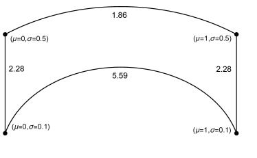
Figure 1: Four normal distributions in the Poincaré half-plane model. Curves represent geodesics and are labeled by the Fisher-Rao distance.

III General Model

We use a simplified form of the Bayesian brain hypothesis [90, 91, 92, 93, 94] to model an individual’s belief using a linear predictor-corrector system

$$\dot{\bm{\theta}}=\bm{\phi}(\bm{\theta},t)+\bm{\chi}(\bm{\theta},\bm{\eta},t).$$ (9)

Here $\bm{\theta}$ are the parameters of the belief distribution $P(\bm{\theta})$ (to be influenced), $\bm{\phi}$ represents the agent’s prediction of how the belief distribution changes over time, and $\bm{\chi}$ represents corrections resulting from the integration of evidence (information) $\bm{\eta}$. While we will not do so here, this linearization could be refined through the addition of $\bm{\phi}\times\bm{\chi}$ cross-terms.

An effective persuasion signal $\bm{\eta}$ will drive the parameters from some initial condition $\bm{\theta}_{0}$ to a final condition $\bm{\theta}_{f}$. The path traversed through probability space has free entropy given by Eq. 3. Consequently, the optimal control problem that minimizes the free entropy is given by

$$\min \frac{1}{2}\int_{t_{0}}^{t_{f}}\mathbf{g}_{jk}(\bm{\theta})\frac{\partial\theta^{j}}{\partial t}\frac{\partial\theta^{k}}{\partial t}\,dt$$ (10)

$$s.t. \dot{\bm{\theta}}=\bm{\phi}(\bm{\theta},t)+\bm{\chi}(\bm{\theta},\bm{\eta},t)$$

$$\bm{\theta}(t_{0})=\bm{\theta}_{0}\quad\bm{\theta}(t_{f})=\bm{\theta}_{f}$$

$$\bm{\eta}\in L^{2}[\mathbb{R}^{k}].$$

However, the action in this case unnecessarily penalizes the natural evolution of the belief as a result of the uncorrected dynamics $\dot{\bm{\theta}}=\bm{\phi}(\bm{\theta},t)$. That is, it is penalizing information that would be expected by a Bayesian brain and therefore already consistent with the belief model.

To model the true cost of persuasion in terms of the inconsistency of inputs with an individual’s naturally time-varying belief function, we must define an action that does not penalize the natural time-evolution of the belief surface. As such, we will use the modified action

$$A_{\chi}=\frac{1}{2}\int_{t_{0}}^{t_{1}}\mathbf{g}_{jk}\chi^{j}\chi^{k}dt,$$ (11)

in Eq. 10.

As with Eq. 3, this action has an information theoretic interpretation. It follows from Eq. 9 that

$$\bm{\theta}(t_{i+1})\approx\bm{\phi}\Delta t+\bm{\chi}\Delta t.$$

Our requirement that the action does not penalize the natural time-evolution of the belief surface corresponds to disregarding changes in $\bm{\theta}$ due to the prediction term $\bm{\phi}$, which represents prior dynamics in the belief process, and only accumulating information from the corrector term $\bm{\chi}$. In other words we wish to minimize the average KL-divergence between the predicted and corrected belief distributions at time $t_{i}$ given by,

$$D_{KL}\left[P(\bm{\theta}(t_{i})+\bm{\phi}\Delta t)\|P(\bm{\theta}(t_{i})+\bm{\phi}\Delta t+\bm{\chi}\Delta t)\right].$$

Using Eq. 5 we have

$$A_{\chi}\approx\sum_{i}\mathbf{g}_{jk}[\bm{\theta}(t_{i})]\chi^{i}\chi^{k}\Delta t\approx\\ \frac{1}{\Delta t}\sum_{i}\mathbf{g}_{jk}[\bm{\theta}(t_{i})+\bm{\phi}\Delta t]\chi^{i}\Delta t\chi^{k}\Delta t\approx\\ \frac{1}{\Delta t}\sum_{i}D_{KL}\left[P(\bm{\theta}(t_{i})+\bm{\phi}\Delta t+\bm{\chi}\Delta t)\|P(\bm{\theta}(t_{i})+\bm{\phi}\Delta t)\right].$$

Thus Eq. 11 measures accumulation of information due to dynamics resulting from the corrector term. In situations where $\bm{\chi}=\bm{0}$ the system will evolve according to its natural predictor dynamics and $A_{\chi}=0$. In situations where $\bm{\phi}=0$, then $A_{\chi}=A$ and we recapture the geodesic interpretation presented previously.

Whether explicit or intuitive, observers often have a threshold for the rate at which they expect to gain information. Aggressive correctors, which cause belief distributions to change quickly so that $A_{\chi}$ is large, are likely to be viewed with suspicion, based on empirical evidence [63]. On the other extreme, if the KL-divergence of an individual step is small enough it may be difficult for the observer to detect the impact of the corrector at all. By optimizing Eq. 11 to achieve an optimal path we can, notionally, change the underlying distribution slowly enough (with respect to the information metric) that the observer is less likely to reject persuasion (or more likely to be susceptible to misinformation).

For the remainder of this paper, we will refer to the optimization problem with action given in Eq. 3 as the geodesic control problem. The optimization problem with action given by Eq. 11 will be referred to as the corrector control problem.

IV Persuasion in the Kalman-Bucy Filter

Kalman filters are archetypal examples of Bayesian filters [95] and as such can be used to model belief/decision processes in neurological systems [94], under a Bayesian brain assumption. More generally, they are also a well established model for perception, particularly in control theory (see e.g., [96]).

Suppose that an object is moving in one dimension with constant velocity $u$ so that

$$\dot{x}=u+w$$

$$z=x+v,$$

where $z$ is the observation and $w\sim N(0,q)$ and $v\sim N(0,r)$. Here $q$ and $r$ are variances. The associated Kalman-Bucy filter [97] produces a distribution estimate $N(\mu,s)$, with

$$\dot{\mu}=u+\frac{s}{r}(z-\mu)$$ (12)

$$\dot{s}=q-\frac{s^{2}}{r},$$ (13)

where $s=\sigma^{2}$ is again a variance. It is straightforward to see how these equations can be written in predictor-corrector form as,

$$\begin{bmatrix}\dot{\mu}\\ \dot{s}\end{bmatrix}=\underbrace{\begin{bmatrix}u\\ q\end{bmatrix}}_{\bm{\phi}}+\underbrace{\begin{bmatrix}\frac{s}{r}(z-\mu)\\ -\frac{s^{2}}{r}\end{bmatrix}}_{\bm{\chi}}.$$

In this problem, the control variables are,

$$\bm{\eta}=\begin{bmatrix}z\\ r\end{bmatrix},$$

since they characterize the observed (input) signal. The persuasive problem in this case is to provide inputs (real or fictitious) to drive the state of belief to some $(\mu_{f},s_{f})$, given an initial belief state $(\mu_{0},s_{0})$. We now consider the problems of finding an optimal input $\bm{\eta}$ in both Eq. 10 and the alternate problem using the action given in Eq. 11.

IV.1 Geodesic Control Problem

We can solve the geodesic control problem in Eq. 10 using Eqs. 7 and 8. Solving Eq. 12 and Eq. 13 in terms of $r$ and $z$ yields,

$$z=\frac{\mu(q-\dot{s})+s(\dot{\mu}-u)}{q-\dot{s}}=\mu+s\frac{\dot{\mu}-u}{q-\dot{s}}.$$

$$r=\frac{s^{2}}{q-\dot{s}}.$$

Here

$$s=\sigma^{2}=2\rho^{2}\operatorname{sech}^{2}[\omega(t-\kappa)].$$

For this solution to be well behaved, we require

$$q-\dot{s}=q+4\rho^{2}\omega\tanh(\omega(t-\kappa))\text{sech}^{2}(\omega(t-\kappa))>0.$$

Therefore,

$$q>\arg\min_{0\leq t\leq T}\left[4\rho^{2}\omega\tanh(\omega(t-\kappa))\text{sech}^{2}(\omega(t-\kappa))\right].$$

The critical points of $q-\dot{s}$ are at

$$t_{1,2}^{*}=\kappa+\frac{\log(2\pm\sqrt{3})}{2\omega}.$$

At these points we have

$$q-\dot{s}\left[\kappa+\frac{\log(2\pm\sqrt{3})}{2\omega}\right]=q\mp\frac{8\rho^{2}\omega}{3\sqrt{3}}.$$

Depending on the sign of $\omega$, the two critical points $t_{1,2}^{*}$ are a (local) maximum and minimum respectively. Assuming $\omega\neq 0$, a simple computation shows that

$$\lim_{t\to\pm\infty}q-\dot{s}(t)=q.$$

Therefore, the critical points must correspond not just to local extrema but to a global maximum and minimum respectively. It follows that a necessary and sufficient condition for the solutions of $r$ and $z$ to be well-behaved (not experience blowup in finite time) is

$$q>\left\lvert\frac{8\rho^{2}\omega}{3\sqrt{3}}\right\rvert.$$ (14)

Notably, this inequality could also be reframed into a condition on the time horizon and is equivalent to

$$(t_{f}-t_{0})>\left(\frac{|\alpha|}{3\sqrt{3}\beta q}\right)^{1/3}$$

where $\alpha$ and $\beta$ are constants determined by the boundary conditions. Observe that the smaller $q$, the larger the minimum possible time horizon $t_{f}-t_{0}$. Intuitively this can be interpreted as very strong priors result in a longer persuasion time.

IV.2 Corrector Control Problem

In contrast, we consider the corrector control problem. Using Eq. 11, we obtain the action,

$$A_{\chi}=\frac{s^{2}}{4r^{2}}+\frac{s(z-\mu)^{2}}{2r^{2}},$$

since the metric written in terms of $s$ (rather than $\sigma$) is,

$$\mathbf{g}=\begin{bmatrix}\frac{1}{s}&0\\ 0&\frac{1}{2s^{2}}\end{bmatrix}.$$

The Hamiltonian for the control system is given as

$$H=A_{\chi}+\lambda\left(u+\frac{s}{r}(z-\mu)\right)+\nu\left(q-\frac{s^{2}}{r}\right),$$ (15)

where $\lambda$ and $\nu$ are Lagrange multipliers (the co-state variables). Setting $H_{\eta}=0$ yields solutions for the inputs,

$$z =\mu-\frac{\lambda}{2\nu}$$ (16)

$$r =\frac{1}{2\nu}.$$ (17)

The resulting Euler-Lagrange equations show that $\dot{\lambda}=0$ and consequently, we define the constant $\lambda(t)=\Lambda$. The remaining Euler-Lagrange equations are,

$$\dot{\mu} =u-\Lambda s$$ (18)

$$\dot{s} =q-2\nu s^{2}$$ (19)

$$\dot{\nu} =\frac{\Lambda^{2}}{2}+2\nu^{2}s.$$ (20)

Notice, $\dot{s}$ and $\dot{\nu}$ are independent of $\mu$ and form a (classical) Hamiltonian system with first integral (mechanical Hamiltonian),

$$\mathcal{H}=\frac{\Lambda^{2}s}{2}-q\nu+\nu^{2}s^{2}.$$ (21)

Here $\mathcal{H}$ is a constant implicitly determined by the boundary conditions (as is $\Lambda$).

While open-loop controls (i.e., functions $z(t)$ and $r(t)$) do not appear to be easily constructed, it is possible to use this information to obtain closed loop controls $z(\mu,s)$ and $r(\mu,s)$. From the Eqs. 16 and 17,

$$z=\mu-\Lambda r.$$

We can use Eq. 21 to construct solutions for $r$ as,

$$r=\frac{-q\pm\sqrt{q^{2}+2s^{2}\zeta(s)}}{2\zeta(s)},$$

where

$$\zeta(s)=2\mathcal{H}-s\Lambda^{2}.$$

We will show numerically that the solution for $r$ switches between the two branches at their point of intersection. That is, at the point in time where,

$$q^{2}+2s^{2}\zeta(s)=0.$$

As we illustrate numerically, this maintains the time-differentiability of $r(t)$.

Notice that $\dot{\nu}>0$ for all time in a physically realistic solution with $s>0$. Moreover, from Eq. 21, we can compute

$$\nu=\frac{-q\pm\sqrt{q^{2}-2s^{2}\zeta(s)}}{2s^{2}}.$$

Since $\nu$ varies inversely with $s^{2}$ and is an increasing function, it follows that when $s$ is small at the boundaries, we may observe stiffness in the ODE, even though solutions exist. That is, the Lagrange multiplier enforcing the variance dynamics is easier to violate numerically. We will observe this in the following examples.

The solutions for $r$ and $\nu$ also imply an existence condition similar to the one in Eq. 14. For an unconstrained optimal control to exist, we must have,

$$q^{2}\geq|2s^{2}\zeta(s)|.$$

Again, this suggests that strong priors can cause difficulty in changing belief functions.

Finally, in both the geodesic control case and the corrector control case, $z$ tracks $\mu$. However, in the corrector control case the $\mu$ tracking is modified by a $-\Lambda r$ term, where the sign of $\Lambda$ will be determined by the goal $\mu_{f}$ and its relation to the natural change in $\mu(t)$ as a result of the given value $u$.

IV.3 Examples

We compare the geodesic control and the corrector control solutions numerically on two example problems. In both cases we assume $\mu(0)=0$, $\mu(1)=1$, and $s(0)=s(1)=0.1$. That is, the objective is to persuade an observer that $\mu(1)=1$ and $s(1)=0.1$, given the initial conditions and the priors, which vary in the two examples. Solution curves are shown in Fig. 2.

Figure 2: Example solutions with $\mu(0)=0$, $\mu(1)=1$, and $s(0)=s(1)=0.1$. (Top) The prior information is $u=1$ and $q=1$. (Bottom) The prior information is $u=-0.5$ and $q=9.5$.

In Fig. 2 (top) we assume the prior information is $u=1$ and $q=1$. That is, the assumed motion dynamics are consistent with the desired end state. We see that both the geodesic controller and the corrector controller both successfully drive the system to the desired end state. However, the corrector controller does so by introducing significantly more variance in to the system. In exchange, the corrector controller trajectory for both $\mu$ and $z$ matches the agent’s prior assumptions on the evolution of $\mu$.

The two branches of the closed loop solution for $r$ are shown in Fig. 3 (top). When compared to Fig. 2 (top, right) it is clear that the solution for $r$ is switching between the two branches at $t=0.5$.

Figure 3: Branches of the closed loop control solution for $r$ to be compared to the corresponding rows in Fig. 2. The two branches are shown in solid and dashed lines respectively. Note that both exhibit a cusp at $t=0.5$ where the switch occurs in the controller.

Interestingly, there are parameter choices for which the geodesic control does not exist while the corrector controller does. Eq. 14 shows that $q_{\text{min}}\approx 0.3334$ for the geodesic controller to exist. Setting $q=0.1$, produces a poorly behaved geodesic controller in which $z$ exhibits blow up in finite time, while $r$ becomes negative. This is shown in Fig. 4.

Figure 4: The solutions for $z$ (top) and $r$ (bottom) in the case when a well-behaved geodesic controller does not exist, but the corrector controller exists.

We contrast this behavior in the next example where parameter classes exist for which the geodesic controller exists but the corrector controller is stiff (and hence a solution exists, but is hard to identify numerically).

In Fig. 2 (bottom) we assume the prior information is $u=-0.5$ and $q=9.5$. That is, the assumed dynamics are inconsistent with the desired end state. The prior $q$ is set large to ensure a control solution exists. Numerical methods show that a minimum value for $q$ is $q_{\text{min}}\approx 8.8343$ to ensure that the corrector controller dynamics are not stiff. If the prior is any stronger, then a numerical solution cannot readily be determined by simple methods. Compare this with the geodesic controller, where Eq. 14 shows that $q_{\text{min}}\approx 0.3334$ for the geodesic controller to exist. Interestingly, simply adjusting the boundary conditions for $s$ (to be larger) removes this stiffness with all other parameters being held constant (this is not shown).

In general, the geodesic controller produces the same parameter path no matter the a priori belief for the velocity. Conversely, the corrector controller is sensitive to the agent’s priors, and produces the most obvious set of inputs when the desired motion matches said priors. In the case of the inconsistent prior, the corrector controller produces a path that starts with high bias, high variance measurements in order to build uncertainty then transitions to low variance measurements over time. In contrast one might argue that the geodesic controller appears to brute force the system by feeding in low variance measurements that drive the parameters along the geodesic.

V Persuasion in a Boltzmann (Softmax) Classifier

Boltzmann distributions and Gibbs measures have been studied in the context of information geometry by several authors in relation to thermodynamics [71, 72, 69, 74, 98] as well as neural networks [82]. In this section, we consider the information geometry of the Boltzmann distribution when treated as a softmax classifier, which measures evidence and provides a probability associated to a specific world state or decision.

Given parameter values $x_{i}$ and a fixed parameter $\beta$, the discrete Boltzmann distribution is,

$$p_{i}=\frac{e^{\beta x_{i}}}{\sum_{j}e^{\beta x_{j}}}.$$ (22)

Here $\beta=(kT)^{-1}$ represents the “inverse temperature” of the system in the statistical physics sense. This distribution is used as the basis for softmax classifiers [85] and also appears in $n$-ary options markets, commonly used in prediction markets [99].

We think of $x_{i}$ as a measure of the evidence supporting conclusion $i$. In this case, controlling the value of $x_{i}$ can be thought of as providing evidence (information in bits or nats) persuading/disuaiding an agent that a certain world state is true. From the perspective of misinformation, this may cause a misclassification and thus is related to (but distinct from) problems in adversarial learning (see, e.g., [100]) when the $x_{i}$ are generated as the penultimate layer of a neural network.

Applying the quotient rule to Eq. 22 yields,

$$\dot{p}_{i}=\sum_{j}\beta p_{i}p_{j}\left(\dot{x}_{i}-\dot{x}_{j}\right).$$

Thus, the dynamics of the distribution depend on the dynamics of the evidence itself. We now assume that the predictor-corrector dynamic is exhibited in the evidence collection process so that,

$$\begin{bmatrix}\dot{x}_{1}\\ \vdots\\ \dot{x}_{n}\end{bmatrix}=\underbrace{\begin{bmatrix}\phi_{1}(\mathbf{x})\\ \vdots\\ \phi_{n}(\mathbf{x})\end{bmatrix}}_{\phi}+\underbrace{\begin{bmatrix}\chi_{1}(\mathbf{x},\bm{\eta})\\ \vdots\\ \chi_{n}(\mathbf{x},\bm{\eta})\end{bmatrix}}_{\chi}.$$

This subsumes (a variation of) the leaky integrator version [101] of the diffusion decision model (DDM) [31] from mathematical neuroscience in which we have

$$\dot{x}_{i}=a_{i}+\alpha_{i}x_{i}+\eta_{i}.$$

When $\alpha_{i}<0$, evidence leaks away (as a process of information aging). If $\alpha_{i}>0$, this models confirmation bias [102] in evidence collection. We note that the DDM model is usually a stochastic differential equation [101, 31] and defer analysis of this more complex case to future work.

Using Hofbauer’s trick [103], let

$$z_{i}=\frac{p_{i}}{p_{n}}\quad\text{and}\qquad q_{i}=\log(z_{i})\iff z_{i}=e^{q_{i}}.$$

Since $p_{1}+\cdots+p_{n}=1$, we can write:

$$p_{n}=\frac{1}{1+\sum_{i=1}^{n-1}e^{q_{i}}}.$$ (23)

Using the quotient rule we see,

$$\dot{z}_{i} =\beta z_{i}\left(\dot{x}_{i}-\dot{x}_{n}\right),$$

$$\dot{q}_{i} =\beta\left(\dot{x}_{i}-\dot{x}_{n}\right).$$

The Fisher pseudo-metric in terms of $\mathbf{p}=\langle{p_{1},\dots,p_{n}}\rangle$ is,

$$\mathbf{g}_{ij}=\begin{cases}\sum_{j\neq i}\beta^{2}p_{i}p_{j}&\text{if $i=j$}\\ -\beta^{2}p_{i}p_{j}&\text{if $i\neq j$}.\end{cases}$$ (24)

The differential form can be computed explicitly, with the Einstein summation convention in the center expression, as

$$ds^{2}=\mathbf{g}_{ij}\,dx^{i}\,dx^{j}=\sum_{i<j}\beta^{2}p_{i}p_{j}\left(dx^{i}-dx^{j}\right)^{2}.$$ (25)

To convert to coordinates in $\mathbf{q}$, note that

$$p_{i}p_{j} =p_{n}^{2}\frac{p_{i}p_{j}}{p_{n}^{2}}=\frac{e^{q_{i}+q_{j}}}{\left(1+\sum_{i=1}^{n-1}e^{q_{i}}\right)^{2}}$$

$$p_{i}p_{n} =p_{n}^{2}\frac{p_{i}}{p_{n}}=\frac{e^{q_{i}}}{\left(1+\sum_{i=1}^{n-1}e^{q_{i}}\right)^{2}}.$$

Finally, if $j\neq n$ we have,

$$(\dot{x}_{i}-\dot{x}_{j})=\frac{\dot{q}_{i}-\dot{q}_{j}}{\beta},$$

which gives the Lagrangian for the geodesic control action $A$ as,

$$\mathcal{L}(\mathbf{q},\dot{\mathbf{q}})=\frac{1}{2\left(1+\sum_{k=1}^{n-1}e^{q_{k}}\right)^{2}}\cdot\\ \left(\sum_{i<j<n}e^{q_{i}+q_{j}}(\dot{q}_{i}-\dot{q}_{j})^{2}+\sum_{j=1}^{n-1}e^{q_{j}}\dot{q}_{j}^{2}\right).$$ (26)

It is straightforward to construct the action for the corrector control action as,

$$\mathcal{L}_{\chi}(\mathbf{q},\bm{\chi})=\frac{1}{2\left(1+\sum_{k=1}^{n-1}e^{q_{k}}\right)^{2}}\cdot\\ \left(\sum_{i<j<n}e^{q_{i}+q_{j}}(\chi_{i}-\chi_{j})^{2}+\sum_{j=1}^{n-1}e^{q_{j}}\chi_{j}^{2}\right),$$ (27)

by simply replacing the dynamics $\dot{q}_{i}$ with its corrector component. Without loss of generality, let $\beta=1$; at this point, it has cancelled out in the Lagrangian and it is simply an extra parameter to carry forward.

V.1 Predictorless Control Problem

In the special case when $\dot{x}_{i}=\eta_{i}$ (i.e., the predictor is zero), the geodesic and corrector control problems are identical. That is $A=A_{\chi}$ and we can use classical techniques from the calculus of variations to find the optimal control.

Deriving the Euler-Lagrange equations for an arbitrary initial and final condition with an arbitrary number of states is cumbersome. However, we can derive an exact solution in the case when we begin from the maximum entropy state,

$$q_{1}(t_{0})=q_{2}(t_{0})=\cdots=q_{n-1}(t_{0})=0$$

and wish to perturb only $q_{1}$ (i.e., we change only $p_{1}$ while all other states are ignored). In this case, we find the optimal path to the state

$$q_{1}(t_{f})=a\quad q_{2}(t_{f})=\cdots=q_{n-1}(t_{f})=0.$$

From this we see that $\dot{q}_{j}=0$ for $j\neq 1$ and the Lagrangian simplifies to

$$\mathcal{L}(\mathbf{q},\dot{\mathbf{q}})=\frac{(n-1)e^{q_{1}}\dot{q}_{1}^{2}}{2\left[(n-1)+e^{q_{1}}\right]^{2}}.$$

Computing the Euler-Lagrange equation and solving for $\ddot{q}_{1}$ yields

$$\ddot{q}_{1}=\frac{\left[e^{q_{1}}+1-n\right]\dot{q}_{1}^{2}}{2\left[(n-1)+e^{q_{1}}\right]},$$

which can be phrased as the system of first order differential equations using the control variable $\eta_{1}$,

$$\left\{\begin{aligned} &\dot{\eta}=\frac{\left[e^{q}+1-n\right]\dot{q}^{2}}{2\left[(n-1)+e^{q}\right]}\\ &\dot{q}=\eta\\ &q(0)=0,q(T)=a,\end{aligned}\right.$$

where we remove the subscripts for readability. Because of the simplicity of the Boltzmann distribution, the units of $\eta$ are naturally in nats (or bits) per time unit.

This system of differential equations has a closed form solution:

$$q(t)=\log\left((n-1)\tan^{2}\left(\frac{1}{2}\sqrt{n-1}(c_{1}t+c_{2})\right)\right)$$ (28)

$$\eta(t)=c_{1}\sqrt{(n-1)\tan^{2}\left(\frac{1}{2}\sqrt{n-1}(c_{1}t+c_{2})\right)}\cdot$$

$$\hskip 60.00009pt\csc^{2}\left(\frac{1}{2}\sqrt{n-1}(c_{1}t+c_{2})\right).$$ (29)

If we assume $t_{f}=1$, the constants are given by,

$$c_{1}=\frac{\cos^{-1}(1-2a)-\cos^{-1}\left(\frac{n-2}{n}\right)}{\sqrt{n-1}},$$

$$c_{2}=\frac{\cos^{-1}\left(\frac{n-2}{n}\right)}{\sqrt{n-1}}.$$

Using the fact that $q_{2}=\cdots q_{n-1}=0$ and Eq. 23, we can compute

$$p_{1}(t) =\sin^{2}\left(\frac{1}{2}\sqrt{n-1}(c_{1}t+c_{2})\right),$$ (30)

$$p_{2}(t) =\cdots=p_{n}(t)=\frac{\cos^{2}\left(\frac{1}{2}\sqrt{n-1}(c_{1}t+c_{2})\right)}{n-1}.$$ (31)

Further, if we assume that $p_{1}(t_{f})>\tfrac{1}{n}$ (i.e., $q(t_{f})>0$), then $\eta(t)>0$ and we use the positive branch of the square root in Eq. 29 to find the simpler expression,

$$\eta(t)=2c_{1}\sqrt{n-1}\csc\left(\sqrt{n-1}(c_{1}t+c_{2})\right).$$

If the opposite is true, then we simply use the negative branch and $\eta(t)$ is the negative of this quantity.

In the edge case when $n=2$, these results simplify substantially to,

$$p_{1}(t) =\sin^{2}\left(\frac{1}{2}(c_{1}t+c_{2})\right),$$

$$p_{2}(t) =\cos^{2}\left(\frac{1}{2}(c_{1}t+c_{2})\right),$$

$$\eta(t) =2c_{1}\csc(c_{1}t+c_{2}).$$

We can likewise compute the explicit form of the solution when $n\to\infty$, representing the case of many possible belief states. Then we have,

$$p_{1}(t)=\sin^{2}\left(\frac{1}{2}t\cos^{-1}(1-2a)\right)$$

$$\eta(t)=2\cos^{-1}(1-2a)\csc\left(t\cos^{-1}(1-2a)\right).$$

The control curves and probability paths for a range of $n$ when $p_{1}(t_{f})=0.8$ are illustrated in Fig. 5.

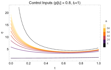
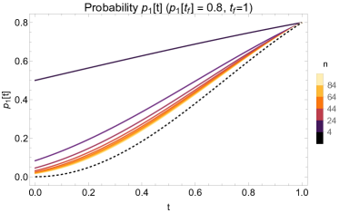
Figure 5: (Top) The control curves for various $n$ ($2\leq n\leq 102$). The black dashed control curve is the asymptotic control when $n\to\infty$. (Bottom) The trajectories of the probability of belief in State 1 given control inputs for various $n$ (as specified). The black dashed curve is the asymptotic behavior of $p_{1}(t)$ as $n\to\infty$. In both figures $t_{0}=0$, $t_{f}=1$, and $p_{1}(t_{f})=0.8$.

Note that these plots do not directly show the path in the parameter space $x_{i}$. Instead we see how the resulting probability changes over time and the rate $\eta$ that information must be supplied to change the probability. First observe that, like previous examples, the rate of change of the probability is fastest when the variance is high and slows near areas of certainty. This is consistent with the Fisher-Rao metric and our expectation that regions of certainty will have higher curvature. On the other hand, the rate at which information must be funneled into the system has its maxima at $t=t_{0}$ and $t=t_{f}$. Indeed the region when the probability is changing the fastest is also the region where the information input is smallest. The nature of the Boltzmann distribution requires increasing energy expenditure to shift distributions towards further certainty. More broadly, reduced utility for persuasion targeted towards strong priors is an important dynamic.

V.2 Leaky Integrator Control Problem

Analyzing the control problem for the Boltzmann distribution when inputs have fully general dynamics requires numerical analysis. However, we can gain insight from the special case when for all $i$, $x_{i}$ follows the dynamic

$$\dot{x}_{i}=\underbrace{a+\alpha x_{i}}_{\phi_{i}}+\underbrace{\eta_{i}}_{\chi_{i}}.$$

That is, we assume all information dynamics share a common predictor model and only the corrector (control) dynamics vary. For simplicity, we will continue to assume that $\beta=1$.

From our previous analysis, we see that

$$\dot{q}_{i}=\alpha(x_{i}-x_{n})+(\eta_{i}-\eta_{n}).$$

Let $\xi_{i}=x_{i}-x_{n}$ and $\zeta_{i}=\eta_{i}-\eta_{n}$. Notice that

$$\dot{\xi}_{i}=\dot{x}_{i}-\dot{x}_{n}=\dot{q}_{i}.$$

Therefore $q_{i}=\xi_{i}+C_{i}$ for some constant $C_{i}$. If we impose a symmetry assumption that all $x_{i}(0)$ are equal, then initially $q_{i}(0)=0=\xi_{i}(0)$ for all $i$. It follows at once that $C_{i}=0$ and $q_{i}=\xi_{i}$ and $q_{i}$ has dynamics

$$\dot{q}_{i}=\alpha q_{i}+\zeta_{i}.$$

That is, in this highly symmetric case, $q_{i}$ inherits the dynamics of $x_{i}$ almost entirely.

If we again assume that we wish to modify only $q_{1}$ then for $i\neq 1$, as before, $\eta_{i}=0$, which implies $\zeta_{i}=0$. Since we assumed that we are starting from a maximum entropy state, we have $q_{i}(0)=0$ and, therefore, $q_{i}(t)=0$ for all time, since $\dot{q}_{i}=0$. For $i=1$, we have $\zeta_{1}=\eta_{1}$ and the resulting simplified Lagrangians for the geodesic case and corrector case in terms of $\eta_{1}$ are:

$$\mathcal{L}(\mathbf{q},\bm{\zeta})=\frac{(n-1)e^{q_{1}}(\alpha q_{1}+\eta_{1})^{2}}{2\left[(n-1)+e^{q_{1}}\right]^{2}}$$

$$\mathcal{L}_{\chi}(\mathbf{q},\bm{\zeta})=\frac{(n-1)e^{q_{1}}\eta_{1}^{2}}{2\left[(n-1)+e^{q_{1}}\right]^{2}}.$$

The dynamics of $q_{1}$ are then,

$$\dot{q}_{1}=\alpha q_{1}+\zeta_{1}=\alpha q_{1}+\eta_{1}.$$

For simplicity, we will discard the subscripts. The Hamiltonians for the two control systems are almost identical,

$$H_{\text{geodesic}}=\frac{(n-1)e^{q}(\alpha q+\eta)^{2}}{2\left[(n-1)+e^{q}\right]^{2}}+\lambda\left(\alpha q+\eta\right)$$

$$H_{\text{corrector}}=\frac{(n-1)e^{q}\eta^{2}}{2\left[(n-1)+e^{q}\right]^{2}}+\lambda\left(\alpha q+\eta\right)$$

The resulting dynamics are similar with,

$$\text{Geodesic}\left\{\begin{aligned} \dot{q}&=-\frac{\lambda e^{-q}\left(n-1+e^{q}\right)^{2}}{n-1}\\ \dot{\lambda}&=\frac{\lambda^{2}\left(n-1+e^{q}\right)}{2(n-1)}\left(1-(n-1)e^{-q}\right)\end{aligned}\right.$$

and

$$\text{Corrector}\left\{\begin{aligned} \dot{q}&=\alpha q-\frac{\lambda e^{-q}\left(n-1+e^{q}\right)^{2}}{n-1}\\ \dot{\lambda}&=-\alpha\lambda+\frac{\lambda^{2}\left(n-1+e^{q}\right)}{2(n-1)}\left(1-(n-1)e^{-q}\right),\end{aligned}\right.$$

where the controls are given by,

$$\eta_{\text{geodesic}}=-\alpha q-\frac{\lambda e^{-q}\left(n-1+e^{q}\right)^{2}}{n-1}$$

$$\eta_{\text{corrector}}=-\frac{\lambda e^{-q}\left(n-1+e^{q}\right)^{2}}{n-1}$$

Notice that $\alpha$ does not appear in the geodesic dynamics. As expected, the geodesic path is not affected by information leakage or bias. This is accounted for by the controller itself. On the other hand, the behavior of the corrector dynamics does include $\alpha$ and consequently the corrector controller will modify the path through probability space to take advantage of (or to compensate for) leakage or bias, even though the leakage/bias term does not appear explicitly in the control law.

The geodesic dynamics do have a (large) closed form solution in elementary functions, but it is not useful as a point of comparison since the corrector controller does not appear to have a convenient closed form solution, even though the system is integrable. A more useful comparison is by numerical example, where we show that the information injected into the system is always less in the corrector controller case (as expected).

Fig. 6 shows the probability path for $p_{1}(t)$ and the control signals for the geodesic and corrector controllers (both in nats per time unit) for the cases when $\alpha=1$ and $\alpha=-1$. It is worth noting that only one probability path is shown because both controllers use a single path. This is expected for the geodesic controller, but appears to be a quirk of the corrector controller, whose solutions are invariant to the sign of $\alpha$. In all cases, the information input per unit time into the system is less for the corrector controller than it is for the geodesic controller.

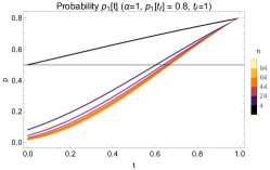
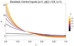
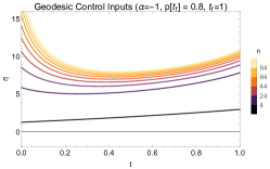
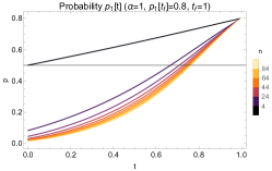
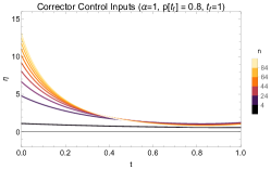
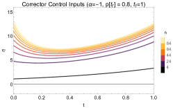
Figure 6: (Left) Controlled probability paths $p_{1}$ for (top) geodesic controller, (bottom) corrector controller. (Center) Controller inputs $\eta$ for (top) geodesic controller, (bottom) corrector controller, when $\alpha=1$, modeling bias. (Right) Controller inputs $\eta$ for (top) geodesic controller, (bottom) corrector controller, when $\alpha=-1$, modeling information leakage.

Interestingly, in the case when $\alpha=1$, the information input in the geodesic controller actually becomes negative (which is allowed in the DDM) to compensate for the biasing affect and to keep the probability following the geodesic. This does not happen in the corrector controller case, which uses the bias to its advantage. In a real-world scenario, negative information would correspond to some kind of counter-factual evidence supporting a specific world state (or information supporting one of the other $n-1$ world states). In the case when $\alpha=-1$, both controllers decrease and then increase their information rates to compensate for the information leakage.

VI A Rudimentary Fusion Model

The building blocks described above can be combined to produce more complicated models using the underlying information geometry. An important fact is that given two parameterized probability distributions $p_{1}(\mathbf{x}|\bm{\theta})$ and $p_{2}(\mathbf{x}|\bm{\theta})$ with associated Fisher-Rao metrics $\mathbf{g}^{1}$ and $\mathbf{g}^{2}$, respectively, then the Fisher-Rao metric for the product distribution $p_{1}(\mathbf{x}_{1}|\bm{\theta})p_{2}(\mathbf{x}_{2}|\bm{\theta})$ is given by

$$\mathbf{g}(\bm{\theta})=\mathbf{g}^{1}(\bm{\theta})+\mathbf{g}^{2}(\bm{\theta}).$$

This follows from direct computation and the fact that

$$\mathbb{E}_{\bm{\theta}}\left[\frac{\partial p(\mathbf{x}|\bm{\theta})}{\partial\bm{\theta}}\right]=0.$$

Restated in terms of actions and Hamiltonians, this implies that for independent joint distributions we can simply add the actions (geodesic or corrector) associated to each distribution.

By way of example, assume there are $N$ independent one-dimensional Kalman filters as in Section IV with belief parameters $(\mu_{k},s_{k})$, observed mean and variance and $(z_{k},r_{k})$, acting as control variables, and priors $(u_{k},q_{k})$. Here $k\in\{1,\dots,N\}$. For filter $k$ we have a Hamiltonian $H_{k}$ given by Eq. 15, with the appropriate set of parameters.

An individual may wish to know which (if any) of the Kalman trackers represents a real trajectory (vs. spuriously coherent noise). Such a scenario may occur, e.g., in the visual systems of predators who are attempting to isolate prey trajectories from clutter. (See [94], for supporting evidence that Kalman filters are adequate models of visually guided pursuit dynamics.)

A reasonable assumption is that the agent is using the variance of the perceived position as evidence for a Boltzmann distribution indicating which of the Kalman filters represents the more likely (real) trajectory. Specifically suppose the probability that filter $k$ is the true track is given by Eq. 22 where the evidence for filter $k$ is the negative entropy associated to the observed position. While the entropy of a normal distribution with variance $s$ is given by $\frac{1}{2}\log(2\pi es)$, we will disregard the unimportant constant factors and define

$$x_{k}=-\log(s_{k}).$$ (32)

In this model, more variance leads to higher entropy implying a smaller probability of associating a signal with a true track.

Using Eq. 13, we can split the time derivative of $x_{k}$ into predictor and corrector terms as,

$$\dot{x}_{k}=\frac{-\dot{s}_{k}}{s_{k}}=\underbrace{\frac{-q_{k}}{s_{k}}}_{\phi}+\underbrace{\frac{s_{k}}{r_{k}}}_{\chi},$$

with the control variable being $r_{k}$ as before. As we are taking a numerical approach there is no need to use Hofbauer’s trick in this case. The Hamiltonian associated to the Boltzmann distribution can be read directly from Eqs. 22, 25 and 32 as,

$$H_{0}=\sum_{i<j}\beta^{2}p_{i}p_{j}\left(\frac{s_{i}}{r_{i}}-\frac{s_{j}}{r_{j}}\right)^{2}=\\ \sum_{i<j}\frac{\beta^{2}s_{i}^{-\beta}s_{j}^{-\beta}}{\left(\sum_{k}s_{k}^{-\beta}\right)^{2}}\left(\frac{s_{i}}{r_{i}}-\frac{s_{j}}{r_{j}}\right)^{2}.$$

Note this Hamiltonian has no Lagrange multipliers because we have used Eq. 22 to remove $p_{i}$ from the expression. The total system Hamiltonian is then,

$$H=H_{0}+\sum_{k}H_{k}.$$ (33)

Using Eq. 33 we can write down a the Euler-Lagrange differential equations, which can be solved numerically and which provide necessary conditions for an optimal control.

By way of example, consider a scenario in which the objective is to generate inputs to persuade an observer that one of two trajectories is real, subject to prior assumptions on the Kalman filters. Assume that the agent has prior belief dynamics defined by $\beta=q_{k}=1$ and $u_{1}=0.9$ and $u_{2}=1.1$. Suppose also that we have the initial conditions

$$\mu_{1}(0)=0\quad s_{1}(0)=0.1$$

$$\mu_{2}(0)=0\quad s_{2}(0)=0.1.$$

Our objective can be accomplished (among other methods) by achieving the final conditions,

$$\mu_{1}(t_{f})=0.9\quad s_{1}(t_{f})=0.5$$

$$\mu_{2}(t_{f})=1.1\quad s_{2}(t_{f})=0.1,$$

which leads to $p_{1}(t_{f})\approx 0.167$ and $p_{2}(t_{f})\approx 0.833$. Thus, the second trajectory has a substantially higher probability of being identified as real. The resulting dynamics are shown in Fig. 7.

Figure 7: (Left) The optimal mean values $\mu_{1}$ and $\mu_{2}$. (Center) The optimal variances $s_{1}$ and $s_{2}$. (Right) The probability of assuming path $i$ contains a true trajectory.

While the results are largely unsurprising, there are some interesting characteristics. First note that the optimal mean values $\mu_{k}$ follow linear paths and, as a consequence of the desired final state agreeing with the prior assumptions on $u_{k}$, the control inputs $z_{k}$ follow the same paths (not shown). Also, there is an asymmetry in the $s_{1}$ variance, which has not been seen before and is most likely being induced by the introduction of the $H_{0}$ Hamiltonian elements. As before, however, variance increases and then decreases, with the uncertainty adjusting the curvature of the manifold and thus impacting the distance traversed. The probability results are unintuitive in that the rate of change of the probability appears to be accelerating in regions of higher certainty, where the metric will be more costly. However, this may be a function of choosing a small $\beta$, which (in essence) is now acting as a conversion parameter between the cost associated with the Fisher metric for the Boltzmann distribution and the Fisher metrics for the Kalman filters. Further study of these joint metrics is a direction of future research.

VII Conclusions and Future Directions

In this paper, we present a mathematical model of optimal persuasion, based on psychological models used in learning theory and in understanding misinformation. Our approach formalizes the required notion of familiarity by phrasing the problem in terms of the manipulation of a belief distribution. Familiarity is then couched in terms of free entropy and the Fisher-Rao metric is both used and modified to characterize a path of ‘greatest familiarity’ (least surprise). In particular, we develop a modified Lagrangian that takes into account natural time-varying dynamics of the belief probability distribution in the absence of intentional control (or manipulation). We compare control signals produced using the Fisher-Rao metric to this modified metric for two classic distributions: the Kalman filter and the Boltzmann distribution, modeling an agent attempting to classify a world state. We then showed how to combine these systems to model a rudimentary information fusion system for a single real object in a cluttered field.

There are several future directions of research that may result from this work. In the first case, a closer integration of the mathematical models with classical models from the neuroscience literature, including those incorporating stochasticity would result in a richer understanding of learning/influence in decision making circumstances. This could include experimental validation of the underlying Fisher-Rao metric as a reasonable (component of) a metric for optimizing persuasion. Other richer models may also consider additional terms in the objective function of the control problem. These terms might incorporate the cost of injecting information into the system (either as a part of the learning process or a malicious misinformation process). Relating this work to (online) adversarial learning in machine learning may also be a fruitful area of research. Additionally, further study of joint distribution models may lead to insights into learning or misinformation in complex decision frameworks. Finally, an empirical study of simple misinformation or learning in the context of the (time-varying) distributions presented here would determine the validity of this model and our underlying assumption that the Fisher-Rao metric is a good representation of neurological “familiarity” and thus relevant in learning or influence.

Appendix A Review of Optimal Control

We present key facts from optimal control theory used in this study. Details are available in [104, 88, 105].

A Bolza type optimal control problem is an optimization problem of the form:

$$\left\{\begin{aligned} \min\;\;&\Psi(\mathbf{x}(t_{f}))+\int_{t_{0}}^{t_{f}}f(\mathbf{x}(t),\mathbf{u}(t),t)dt\\ s.t.\;\;&\mathbf{\dot{x}}=\mathbf{g}(\mathbf{x}(t),\mathbf{u}(t),t)\\ &\mathbf{x}(0)=\mathbf{x}_{0}\end{aligned}\right.$$ (34)

When $\Psi(\mathbf{x}(t_{f}))\equiv 0$, this is called a Lagrange type optimal control problem. The vector of variables $\mathbf{x}$ is called the state, while the vector of decision variables $\mathbf{u}$ is called the control. Additional constraints on $\mathbf{u}$, $\mathbf{x}$ or the joint function of $\mathbf{x}$ and $\mathbf{u}$ can be added.

The Hamiltonian with adjoint variables (Lagrange multipliers) $\bm{\lambda}$ for this problem is:

$$\mathcal{H}(\mathbf{x},\bm{\lambda},u)=f(\mathbf{x}(t),\mathbf{u}(t),t)+\bm{\lambda}^{T}\mathbf{g}(\mathbf{x}(t),\mathbf{u}(t),t)$$

In what follows, we assume that all $f(\mathbf{x},\mathbf{u},t)$ and $\mathbf{g}(\mathbf{x},\mathbf{u},t)$ are continuous and differentiable in $\mathbf{x}$ and $\mathbf{u}$ and $\Psi(\mathbf{x}(t_{f}))$ is continuous and differentiable in $x(t_{f})$. A proof of the following lemma can be found in almost every book on optimal control (e.g. [105]).

Lemma A.1 (Necessary Conditions of Optimal Control).

If $\mathbf{u}^{*}$ is a solution to Optimal Control Problem (34), then there is a vector of adjoint variables $\bm{\lambda}^{*}$ so that:

$$\mathcal{H}(\mathbf{x}^{*}(t),\mathbf{u}^{*}(t),\bm{\lambda}^{*}(t))\leq\mathcal{H}(\mathbf{x}^{*}(t),\mathbf{u}(t),\bm{\lambda}^{*}(t))$$ (35)

for all $t\in[0,T]$ and for all admissible inputs $\mathbf{u}$, and the following conditions hold:

1. Pontryagin’s Minimim Principle: $\frac{\partial\mathcal{H}}{\partial\mathbf{u}}=\mathbf{0}$ and $\frac{\partial^{2}\mathcal{H}}{\partial\mathbf{u}^{2}}$ is positive definite,

2. Co-State Dynamics:

   $$\dot{\bm{\lambda}}(t)=-\frac{\partial\mathcal{H}}{\partial\mathbf{x}}=-\bm{\lambda}^{T}(t)\frac{\partial\mathbf{g}(\mathbf{x},\mathbf{u})}{\partial\mathbf{x}}-\frac{\partial f(\mathbf{x},\mathbf{u})}{\partial\mathbf{x}},$$

3. State Dynamics: $\dot{\mathbf{x}}(t)=\frac{\partial\mathcal{H}}{\partial\bm{\lambda}}=\mathbf{g}(\mathbf{x},\mathbf{u})$,

4. Initial Condition: $\mathbf{x}(0)=\mathbf{x}_{0}$, and

5. Transversality Condition: $\bm{\lambda}(t_{f})=\frac{\partial\Psi}{\partial\mathbf{x}}(\mathbf{x}(t_{f}))$.

We note that if a terminal condition $\mathbf{x}(t_{f})$ is given, the transversality condition can be ignored in the necessary conditions.

References

- O’keefe [2015] D. J. O’keefe, Persuasion: Theory and research (Sage Publications, 2015).
- Cervin and Henderson [1961] V. B. Cervin and G. Henderson, Statistical theory of persuasion., Psychological Review 68, 157 (1961).
- Burgoon et al. [1981] J. K. Burgoon, M. Burgoon, G. R. Miller, and M. Sunnafrank, Learning theory approaches to persuasion, Human Communication Research 7, 161 (1981).
- Curtis and Smith [2008] J. P. Curtis and F. T. Smith, The dynamics of persuasion, Int. J. Math. Models Methods Appl. Sci 2, 115 (2008).
- DeGroot [1974] M. H. DeGroot, Reaching a consensus, J. American Stat. Association 69, 118 (1974).
- Krause [2000] U. Krause, A discrete nonlinear and non-autonomous model of consensus formation, in In Communications in Difference Equations, edited by Gordon and Breach (2000) pp. 227– 236.
- Hegselmann and Krause [2002] R. Hegselmann and U. Krause, Opinion dynamics and bounded confidence: Models, analysis and simulation, J. Artificial Soc. Social Simul. 5 (2002).
- Ben-Naim [2005] E. Ben-Naim, Opinion dynamics: Rise and fall of political parties, Europhys. Lett. 69, 671 (2005).
- Weisbuch et al. [2005] G. Weisbuch, G. Deffuant, and F. Amblard, Persuasion dynamics, Physica A 353 (2005).
- Toscani [2006] G. Toscani, Kinetic models of opinion formation, Commun. Math. Sci. 4, 481 (2006).
- Weisbuch [2006] G. Weisbuch, Social opinion dynamics, in Econophysics and Sociophysics: Trends and Perspectives, edited by B. K. Chakrabarti, A. Chakrabarti, and A. Chatterjee (Wiley, 2006) pp. 67–94.
- Lorenz [2007] J. Lorenz, Continuous opinion dynamics of multidimensional allocation problems under bounded confidence. a survey, Internat. J. Modern Phys. C 18, 1819 (2007).
- Blondel et al. [2009] V. D. Blondel, J. M. Hendrickx, and J. N. Tsitsiklis, On krause’s multi-agent consensus model with state-dependent connectivity, IEEE Transactions on Automatic Control 54, 2586 (2009).
- Castellano et al. [2009] C. Castellano, S. Fortunato, and V. Loreto, Statistical physics of social dynamics, Reviews of modern physics 81, 591 (2009).
- Kurz and Rambau [2011] S. Kurz and J. Rambau, On the hegselmann-krause conjecture in opinion dynamics, J. Difference Equ. Appl. 17, 859 (2011).
- Duering et al. [2012] B. Duering, P. Markowich, J. F. Pietschmann, and M. T. Wolfram, Boltzmann and Fokker-Planck equations modelling opinion formation in the presence of strong leaders, Proc. R. Soc. Lond. Ser. A 465 (2012).
- Canuto et al. [2012] C. Canuto, F. Fagnani, and P. Tilli, An eulerian approach to the analysis of krause’s consensus models, SIAM J. Contr. and Opt. , 243 (2012).
- Jabin and Motsch [2014] P.-E. Jabin and S. Motsch, Clustering and asymptotic behavior in opinion formation, Journal of Differential Equations 257, 4165 (2014).
- Shang et al. [2021] L. Shang, M. Zhao, J. Ai, and Z. Su, Opinion evolution in the sznajd model on interdependent chains, Physica A: Statistical Mechanics and its Applications 565, 125558 (2021).
- Glass and Glass [2021] C. A. Glass and D. H. Glass, Opinion dynamics of social learning with a conflicting source, Physica A: Statistical Mechanics and its Applications 563, 125480 (2021).
- Centola and Baronchelli [2015] D. Centola and A. Baronchelli, Flocks, herds, and schools: A quantitative theory of flocking, Proceedings of the National Academy of Sciences 112, 1989 (2015).
- Toner and Tu [1998] J. Toner and Y. Tu, Flocks, herds, and schools: A quantitative theory of flocking, Physical Review E 58, 4828 (1998).
- Cucker and Smale [2007] F. Cucker and S. Smale, Emergent behavior in flocks, IEEE Transactions on Automatic Control 52, 852 (2007).
- Edelstein-Keshet [2001] L. Edelstein-Keshet, Mathematical models of swarming and social aggregation, in Proc. 2001 International Symposium on Nonlinear Theory and Its Applications (NOLTA 2001) (Miyagi, Japan, 2001).
- Li [2008] W. Li, Stability analysis of swarms with general topology, IEEE Trans. Systems, Man and Cybernetics, Part B 38, 1084 (2008).
- Li and Xiao [2010] X. Li and J. Xiao, Swarming in homogeneous environments: A social interaction based framework, J. Theoret. Biol. 264, 747 (2010).
- Degond and Motsch [2011] P. Degond and S. Motsch, A macroscopic model for a system of swarming agents using curvature control, J. Stat. Phys. 143 (2011).
- Motsch and Tadmor [2014] S. Motsch and E. Tadmor, Heterophilious Dynamics Enhances Consensus, SIAM Review 56, 577 (2014).
- Griffin et al. [2022] C. Griffin, A. Squicciarini, and F. Jia, Consensus in complex networks with noisy agents and peer pressure, Physica A: Statistical Mechanics and its Applications 608, 128263 (2022).
- Huang et al. [2016] W.-M. Huang, L.-J. Zhang, X.-J. Xu, and X. Fu, Contagion on complex networks with persuasion, Scientific reports 6, 23766 (2016).
- Ratcliff and McKoon [2008] R. Ratcliff and G. McKoon, The diffusion decision model: theory and data for two-choice decision tasks, Neural computation 20, 873 (2008).
- Xie et al. [2021] H. Xie, M. Zhong, Y. Li, and J. C. Lui, Understanding persuasion cascades in online product rating systems: Modeling, analysis, and inference, ACM Transactions on Knowledge Discovery from Data (TKDD) 15, 1 (2021).
- Kamenica and Gentzkow [2011] E. Kamenica and M. Gentzkow, Bayesian persuasion, American Economic Review 101, 2590 (2011).
- Babichenko et al. [2021] Y. Babichenko, I. Talgam-Cohen, and K. Zabarnyi, Bayesian persuasion under ex ante and ex post constraints, in Proceedings of the AAAI Conference on Artificial Intelligence, Vol. 35 (2021) pp. 5127–5134.
- Caballero and Lunday [2019] W. N. Caballero and B. J. Lunday, Influence modeling: Mathematical programming representations of persuasion under either risk or uncertainty, European Journal of Operational Research 278, 266 (2019).
- Altay et al. [2023] S. Altay, M. Berriche, and A. Acerbi, Misinformation on misinformation: Conceptual and methodological challenges, Social Media+ Society 9, 20563051221150412 (2023).
- Del Vicario et al. [2016] M. Del Vicario, A. Bessi, F. Zollo, F. Petroni, A. Scala, G. Caldarelli, H. E. Stanley, and W. Quattrociocchi, The spreading of misinformation online, Proceedings of the national academy of Sciences 113, 554 (2016).
- Vraga and Bode [2020] E. K. Vraga and L. Bode, Defining misinformation and understanding its bounded nature: Using expertise and evidence for describing misinformation, Political Communication 37, 136 (2020).
- Edelman [2001] M. Edelman, The politics of misinformation (Cambridge University Press, 2001).
- Jerit and Zhao [2020] J. Jerit and Y. Zhao, Political misinformation, Annual Review of Political Science 23, 77 (2020).
- Swire-Thompson et al. [2020] B. Swire-Thompson, D. Lazer, et al., Public health and online misinformation: challenges and recommendations, Annu Rev Public Health 41, 433 (2020).
- Southwell et al. [2019] B. G. Southwell, J. Niederdeppe, J. N. Cappella, A. Gaysynsky, D. E. Kelley, A. Oh, E. B. Peterson, and W.-Y. S. Chou, Misinformation as a misunderstood challenge to public health, American journal of preventive medicine 57, 282 (2019).
- Roozenbeek et al. [2020] J. Roozenbeek, C. R. Schneider, S. Dryhurst, J. Kerr, A. L. Freeman, G. Recchia, A. M. Van Der Bles, and S. Van Der Linden, Susceptibility to misinformation about covid-19 around the world, Royal Society open science 7, 201199 (2020).
- Joseph et al. [2022] A. M. Joseph, V. Fernandez, S. Kritzman, I. Eaddy, O. M. Cook, S. Lambros, C. E. J. Silva, D. Arguelles, C. Abraham, N. Dorgham, et al., Covid-19 misinformation on social media: a scoping review, Cureus 14 (2022).
- Gisondi et al. [2022] M. A. Gisondi, R. Barber, J. S. Faust, A. Raja, M. C. Strehlow, L. M. Westafer, and M. Gottlieb, A deadly infodemic: social media and the power of covid-19 misinformation (2022).
- Whitehead et al. [2023] H. S. Whitehead, C. E. French, D. M. Caldwell, L. Letley, and S. Mounier-Jack, A systematic review of communication interventions for countering vaccine misinformation, Vaccine (2023).
- Neely et al. [2022] S. R. Neely, C. Eldredge, R. Ersing, and C. Remington, Vaccine hesitancy and exposure to misinformation: a survey analysis, Journal of general internal medicine , 1 (2022).
- Enders et al. [2022] A. M. Enders, J. Uscinski, C. Klofstad, and J. Stoler, On the relationship between conspiracy theory beliefs, misinformation, and vaccine hesitancy, Plos one 17, e0276082 (2022).
- Cook [2022] J. Cook, Understanding and countering misinformation about climate change, Research Anthology on Environmental and Societal Impacts of Climate Change , 1633 (2022).
- Zhou and Shen [2022] Y. Zhou and L. Shen, Confirmation bias and the persistence of misinformation on climate change, Communication Research 49, 500 (2022).
- Freiling and Matthes [2023] I. Freiling and J. Matthes, Correcting climate change misinformation on social media: Reciprocal relationships between correcting others, anger, and environmental activism, Computers in Human Behavior 145, 107769 (2023).
- Cook et al. [2015] J. Cook, U. Ecker, and S. Lewandowsky, Misinformation and how to correct it, Emerging trends in the social and behavioral sciences: An interdisciplinary, searchable, and linkable resource , 1 (2015).
- Van der Linden et al. [2017a] S. Van der Linden, E. Maibach, J. Cook, A. Leiserowitz, and S. Lewandowsky, Inoculating against misinformation, Science 358, 1141 (2017a).
- Van der Linden et al. [2017b] S. Van der Linden, A. Leiserowitz, S. Rosenthal, and E. Maibach, Inoculating the public against misinformation about climate change, Global challenges 1, 1600008 (2017b).
- Tay et al. [2022] L. Q. Tay, M. J. Hurlstone, T. Kurz, and U. K. Ecker, A comparison of prebunking and debunking interventions for implied versus explicit misinformation, British Journal of Psychology 113, 591 (2022).
- Ecker et al. [2023] U. K. Ecker, C. X. Sharkey, and B. Swire-Thompson, Correcting vaccine misinformation: A failure to replicate familiarity or fear-driven backfire effects, Plos one 18, e0281140 (2023).
- Schmid-Petri and Bürger [2022] H. Schmid-Petri and M. Bürger, The effect of misinformation and inoculation: Replication of an experiment on the effect of false experts in the context of climate change communication, Public Understanding of Science 31, 152 (2022).
- Buczel et al. [2022] M. Buczel, P. D. Szyszka, A. Siwiak, M. Szpitalak, and R. Polczyk, Vaccination against misinformation: The inoculation technique reduces the continued influence effect, Plos one 17, e0267463 (2022).
- Faisal and Mahendra [2022] D. R. Faisal and R. Mahendra, Two-stage classifier for covid-19 misinformation detection using bert: a study on indonesian tweets, arXiv preprint arXiv:2206.15359 (2022).
- Shao et al. [2022] Y. Shao, J. Sun, T. Zhang, Y. Jiang, J. Ma, and J. Li, Fake news detection based on multi-modal classifier ensemble, in Proceedings of the 1st International Workshop on Multimedia AI against Disinformation (2022) pp. 78–86.
- Fenza et al. [2023] G. Fenza, M. Gallo, V. Loia, A. Petrone, and C. Stanzione, Concept-drift detection index based on fuzzy formal concept analysis for fake news classifiers, Technological Forecasting and Social Change 194, 122640 (2023).
- Mosallanezhad et al. [2022] A. Mosallanezhad, M. Karami, K. Shu, M. V. Mancenido, and H. Liu, Domain adaptive fake news detection via reinforcement learning, in Proceedings of the ACM Web Conference 2022 (2022) pp. 3632–3640.
- Ecker et al. [2022] U. K. Ecker, S. Lewandowsky, J. Cook, P. Schmid, L. K. Fazio, N. Brashier, P. Kendeou, E. K. Vraga, and M. A. Amazeen, The psychological drivers of misinformation belief and its resistance to correction, Nature Reviews Psychology 1, 13 (2022).
- Reynolds [2020] R. M. Reynolds, Why Does Misinformation Persist? Cognitive Explanations of the Implicit Message Effect (Michigan State University, 2020).
- Walter and Tukachinsky [2020] N. Walter and R. Tukachinsky, A meta-analytic examination of the continued influence of misinformation in the face of correction: How powerful is it, why does it happen, and how to stop it?, Communication research 47, 155 (2020).
- Sindermann et al. [2020] C. Sindermann, A. Cooper, and C. Montag, A short review on susceptibility to falling for fake political news, Current Opinion in Psychology 36, 44 (2020).
- Chaxel [2022] A.-S. Chaxel, How misinformation taints our belief system: A focus on belief updating and relational reasoning, Journal of Consumer Psychology 32, 370 (2022).
- Blake and Mullin [2014] I. F. Blake and R. C. Mullin, The mathematical theory of coding (Academic Press, 2014).
- Crooks [2007] G. E. Crooks, Measuring thermodynamic length, Physical Review Letters 99, 100602 (2007).
- Bordel [2011] S. Bordel, Non-equilibrium statistical mechanics: partition functions and steepest entropy increase, Journal of Statistical Mechanics: Theory and Experiment 2011, P05013 (2011).
- Still et al. [2012] S. Still, D. A. Sivak, A. J. Bell, and G. E. Crooks, Thermodynamics of prediction, Physical review letters 109, 120604 (2012).
- Sivak and Crooks [2012] D. A. Sivak and G. E. Crooks, Thermodynamic metrics and optimal paths, Physical review letters 108, 190602 (2012).
- Kim et al. [2016] E.-j. Kim, U. Lee, J. Heseltine, and R. Hollerbach, Geometric structure and geodesic in a solvable model of nonequilibrium process, Physical Review E 93, 062127 (2016).
- Feng and Crooks [2009] E. H. Feng and G. E. Crooks, Far-from-equilibrium measurements of thermodynamic length, Physical review E 79, 012104 (2009).
- Kim and Hollerbach [2017] E.-j. Kim and R. Hollerbach, Geometric structure and information change in phase transitions, Physical Review E 95, 062107 (2017).
- Kim [2021] E.-j. Kim, Information geometry and non-equilibrium thermodynamic relations in the over-damped stochastic processes, Journal of Statistical Mechanics: Theory and Experiment 2021, 093406 (2021).
- Gomez et al. [2020] I. S. Gomez, M. Portesi, and E. P. Borges, Universality classes for the fisher metric derived from relative group entropy, Physica A: Statistical Mechanics and its Applications 547, 123827 (2020).
- Nicholson et al. [2020] S. B. Nicholson, L. P. García-Pintos, A. del Campo, and J. R. Green, Time–information uncertainty relations in thermodynamics, Nature Physics 16, 1211 (2020).
- Fujiwara and Amari [1995] A. Fujiwara and S.-i. Amari, Gradient systems in view of information geometry, Physica D: Nonlinear Phenomena 80, 317 (1995).
- Zhang et al. [2020] Z. Zhang, S. Guan, and H. Shi, Information geometry in the population dynamics of bacteria, Journal of Statistical Mechanics: Theory and Experiment 2020, 073501 (2020).
- Polettini and Esposito [2013] M. Polettini and M. Esposito, Nonconvexity of the relative entropy for markov dynamics: A fisher information approach, Physical Review E 88, 012112 (2013).
- Amari [1997] S.-i. Amari, Information geometry of neural networks—an overview—, Mathematics of Neural Networks: Models, Algorithms and Applications , 15 (1997).
- Ollivier et al. [2017] Y. Ollivier, L. Arnold, A. Auger, and N. Hansen, Information-geometric optimization algorithms: A unifying picture via invariance principles, The Journal of Machine Learning Research 18, 564 (2017).
- Kullback and Leibler [1951] S. Kullback and R. A. Leibler, On Information and Sufficiency, The Annals of Mathematical Statistics 22, 79 (1951).
- Bishop [2006] C. M. Bishop, Pattern recognition and machine learning (Springer, New York, NY, 2006).
- Dowty [2018] J. G. Dowty, Chentsov’s theorem for exponential families, Information Geometry 1, 117 (2018).
- Caticha [2015] A. Caticha, The basics of information geometry, in AIP Conference Proceedings, Vol. 1641 (American Institute of Physics, 2015) pp. 15–26.
- Kirk [2004] D. E. Kirk, Optimal control theory: an introduction (Courier Corporation, 2004).
- Cover and Thomas [2005] T. M. Cover and J. A. Thomas, Elements of Information Theory (Wiley, Hoboken, NJ, 2005).
- Rao and Ballard [1999] R. P. Rao and D. H. Ballard, Predictive coding in the visual cortex: a functional interpretation of some extra-classical receptive-field effects, Nature neuroscience 2, 79 (1999).
- Friston [2012] K. Friston, The history of the future of the bayesian brain, NeuroImage 62, 1230 (2012).
- Baltieri and Isomura [2021] M. Baltieri and T. Isomura, Kalman filters as the steady-state solution of gradient descent on variational free energy, arXiv preprint arXiv:2111.10530 (2021).
- Millidge et al. [2021] B. Millidge, A. Tschantz, A. Seth, and C. Buckley, Neural kalman filtering, arXiv preprint arXiv:2102.10021 (2021).
- de Xivry et al. [2013] J.-J. O. de Xivry, S. Coppe, G. Blohm, and P. Lefevre, Kalman filtering naturally accounts for visually guided and predictive smooth pursuit dynamics, Journal of neuroscience 33, 17301 (2013).
- Meinhold and Singpurwalla [1983] R. J. Meinhold and N. D. Singpurwalla, Understanding the kalman filter, The American Statistician 37, 123 (1983).
- Rao [1999] R. P. Rao, An optimal estimation approach to visual perception and learning, Vision research 39, 1963 (1999).
- Lewis et al. [2008] F. Lewis, L. Xie, and D. Popa, Optimal and Robust Estimation, 2nd ed. (CRC Press, 2008).
- Dixit [2020] P. D. Dixit, Thermodynamic inference of data manifolds, Physical Review Research 2, 023201 (2020).
- Gampe and Griffin [2023] H. Gampe and C. Griffin, Dynamics of a binary option market with exogenous information and price sensitivity, Communications in Nonlinear Science and Numerical Simulation 118, 106994 (2023).
- Miller et al. [2020] D. J. Miller, Z. Xiang, and G. Kesidis, Adversarial learning targeting deep neural network classification: A comprehensive review of defenses against attacks, Proceedings of the IEEE 108, 402 (2020).
- Verdonck et al. [2021] S. Verdonck, T. Loossens, and M. G. Philiastides, The leaky integrating threshold and its impact on evidence accumulation models of choice response time (rt)., Psychological Review 128, 203 (2021).
- Nickerson [1998] R. S. Nickerson, Confirmation bias: A ubiquitous phenomenon in many guises, Review of general psychology 2, 175 (1998).
- Hofbauer [1996] J. Hofbauer, Evolutionary dynamics for bimatrix games: A Hamiltonian system?, J. Math. Bio 34, 675 (1996).
- Mangasarian [1966] O. L. Mangasarian, Sufficient conditions for the optimal control of nonlinear systems, SIAM J. Control 4, 139 (1966).
- Friesz [2010] T. Friesz, Dynamic Optimization and Differential Games (Springer, 2010).