Probing spin hydrodynamics on a superconducting quantum simulator

Abstract

Characterizing the nature of hydrodynamical transport properties in quantum dynamics provides valuable insights into the fundamental understanding of exotic non-equilibrium phases of matter. Simulating infinite-temperature transport on large-scale complex quantum systems remains an outstanding challenge. Here, using a controllable and coherent superconducting quantum simulator, we experimentally realize the analog quantum circuit, which can efficiently prepare the Haar-random states, and probe spin transport at infinite temperature. We observe diffusive spin transport during the unitary evolution of the ladder-type quantum simulator with ergodic dynamics. Moreover, we explore the transport properties of the systems subjected to strong disorder or a titled potential, revealing signatures of anomalous subdiffusion in accompany with the breakdown of thermalization. Our work demonstrates a scalable method of probing infinite-temperature spin transport on analog quantum simulators, which paves the way to study other intriguing out-of-equilibrium phenomena from the perspective of transport.

Transport properties of quantum many-body systems driven out of equilibrium are of significant interest in several active areas of modern physics, including the ergodicity of quantum systems Nandkishore and Huse (2015); Agarwal et al. (2015); Žnidarič et al. (2016); Ljubotina et al. (2023) and quantum magnetism Scheie et al. (2021); Žnidarič (2011); Dupont et al. (2021). Understanding these properties is crucial to unveil the non-equilibrium dynamics of isolated quantum systems Bertini et al. (2021); Eisert et al. (2015). One essential property of transport is the emergence of classical hydrodynamics in microscopic quantum dynamics, which shows the power-law tail of autocorrelation functions Bertini et al. (2021). The rate of the power-law decay, referred as to the transport exponent, characterizes the universal classes of hydrodynamics. In $d$-dimensional quantum systems, in addition to generally expected diffusive transport with the exponent $d/2$ in non-integrable systems Peng et al. (2023); Steinigeweg et al. (2014); Schubert et al. (2021), more attentions have been attracted by the anomalous superdiffusive Scheie et al. (2021); Ljubotina et al. (2017); Wei et al. (2022); Joshi et al. (2022); Rosenberg et al. (2023) or subdiffusive transport Agarwal et al. (2015); Žnidarič et al. (2016); Feldmeier et al. (2020); De Nardis et al. (2022); Gromov et al. (2020), with the exponent larger or smaller than $d/2$, respectively.

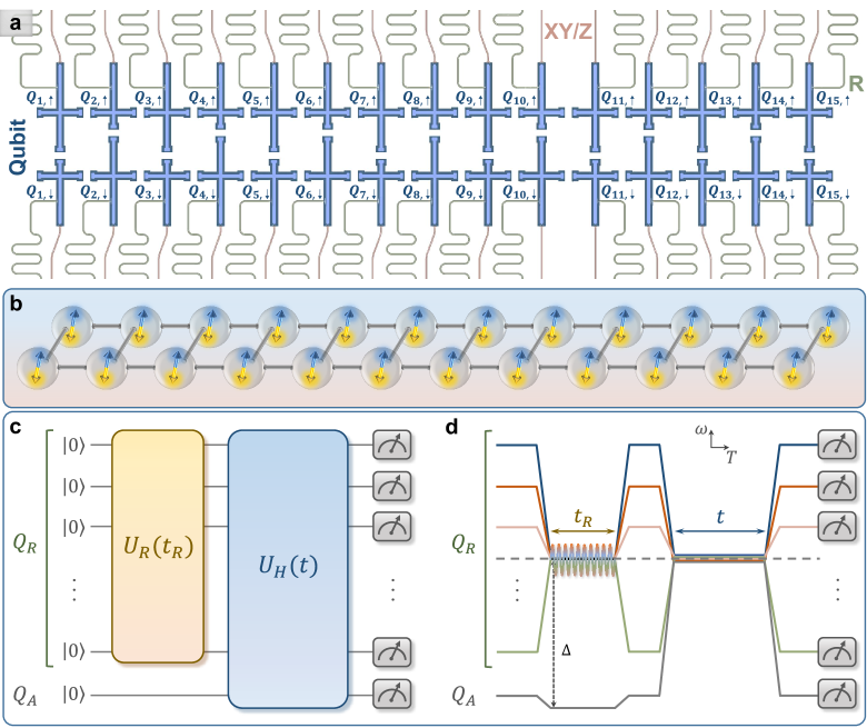
Figure 1: Superconducting quantum simulator and experimental pulse sequences. a, The optical micrograph showing the ladder-type superconducting quantum simulator, consisting of 30 qubits (the blue region), labeled $Q_{1,\uparrow}$ to $Q_{15,\uparrow}$, and $Q_{1,\downarrow}$ to $Q_{15,\downarrow}$. Each qubit is coupled to a separate readout resonator (the green region), and has an individual control line (the red region) for both the XY and Z controls. b, Schematic diagram of the simulated 24 spins coupled in a ladder. The blue and yellow double arrows represent the infinite-temperature spin hydrodynamics without preference for spin orientations. c, Schematic diagram of the quantum circuit for measuring the autocorrelation functions at infinite temperature. All qubits are initialized at the state $|0\rangle$. Subsequently, a pseudo-random circuit $\hat{U}_{R}(t_{R})$ acts on the set of qubits $Q_{R}$. This is followed by a time evolution of all qubits, i.e., $\hat{U}_{H}(t)=\exp(-i\hat{H}t)$ with $\hat{H}$ being the Hamiltonian of the system, in which the properties of spin transport are of our interest. d, Experimental pulse sequences corresponding to the quantum circuit in c, displayed in the frequency ($\omega$) versus time ($T$) domain. To realize $\hat{U}_{R}(t_{R})$, qubits in the set $Q_{R}$ are tuned to the working point (dashed horizontal line) via Z pulses, and simultaneously, the resonant microwave pulses represented as the sinusoidal line are applied to $Q_{R}$ through the XY control lines. Meanwhile, the qubit $Q_{A}$ is detuned from the working point with a large value of the frequency gap $\Delta$. To realize the subsequent evolution $\hat{U}_{H}(t)$ with the Hamiltonian (1), all qubits are tuned to the working point.

Over the last few decades, considerable strides have been made in enhancing the scalability, controllability, and coherence of noisy intermediate-scale quantum (NISQ) devices based on superconducting qubits. With these advancements, several novel phenomena in non-equilibrium dynamics of quantum many-body systems have been observed, such as quantum thermalization Chen et al. (2021); Zhu et al. (2022), ergodicity breaking Roushan et al. (2017); Guo et al. (2021a, b); Zhang et al. (2023), time crystal Zhang et al. (2022); Mi et al. (2022); Frey and Rachel (2022), and information scrambling Mi et al. (2021); Braumüller et al. (2022). More importantly, in this platform, the quantum advantage has been demonstrated by sampling the final Haar-random states of randomized sequences of gate operations Neill et al. (2018); Boixo et al. (2018); Arute et al. (2019); Wu et al. (2021); Morvan et al. (2023). Recently, a method of measuring autocorrelation functions at infinite temperature based on the Haar-random states has been proposed, which opens up a practical application of pseudo-random quantum circuits for simulating hydrodynamics on NISQ devices Richter and Pal (2021); Keenan et al. (2023).

In this work, using a ladder-type superconducting quantum simulator with up to 24 qubits, we first demonstrate that in addition to the digital pseudo-random circuits Neill et al. (2018); Boixo et al. (2018); Arute et al. (2019); Wu et al. (2021); Morvan et al. (2023); Richter and Pal (2021); Keenan et al. (2023), a unitary evolution governed by a time-independent Hamiltonian, i.e., an analog quantum circuit, can also build up the necessary randomness for measuring the infinite-temperature autocorrelation functions C. et al. (2023). Subsequently, we study the properties of spin transport on the superconducting quantum simulator via the measurement of autocorrelation functions by using the Haar-random states. Notably, we observe a clear signature of the diffusive transport on the qubit ladder, which is a non-integrable system Steinigeweg et al. (2014); Schubert et al. (2021).

Upon subjecting the qubit ladder to disorder, a transition from delocalized phases to the many-body localization (MBL) occurs as the strength of disorder increases Sun et al. (2020). By measuring the autocorrelation functions, we experimentally probe an anomalous subdiffusive transport with intermediate values of the disorder strength. The observed signs of subdiffusion are consistent with recent numerical results, and can be explained as a consequence of Griffth-like region on the delocalized side of the MBL transition Agarwal et al. (2015); Žnidarič et al. (2016); Khait et al. (2016); Gopalakrishnan et al. (2016); Setiawan et al. (2017); Luitz and Lev (2017).

Finally, we explore spin transport on the qubit ladder with a linear potential, and it is expected that Stark MBL occurs when the potential gradients are sufficiently large Guo et al. (2021b); Morong et al. (2021); Guo et al. (2021b); Schulz et al. (2019); van Nieuwenburg et al. (2019); Wang et al. (2021); Taylor et al. (2020). With a large gradient, the conservation of the dipole moment emerges Guo et al. (2021b); Taylor et al. (2020), associated with the phenomena known as the Hilbert space fragmentation Doggen et al. (2021); Khemani et al. (2020); Sala et al. (2020). Recent theoretical works reveal a subdiffusion in the dipole-moment conserving systems Feldmeier et al. (2020); Gromov et al. (2020). In this experiment, we present evidence of a subdiffusive regime of spin transport in the titled qubit ladder.

Experimental setup and protocol

Our experiments are performed on a programmable superconducting quantum simulator, consisting of 30 transmon qubits with a geometry of two-legged ladder, see Fig. 1a and b. The nearest-neighbor qubits are coupled by a fixed capacitor, and the effective Hamiltonian of capacitive interactions can be written as Xiang et al. (2023); Gu et al. (2017) (also see Supplementary Section I)

$$\hat{H}_{I}/\hbar = \sum_{m\in\{\uparrow,\downarrow\}}\sum_{j=1}^{L-1}J^{\parallel}_{j,m}(\hat{\sigma}_{j,m}^{+}\hat{\sigma}_{j+1,m}^{-}+\text{H.c.})$$ (1)

$$+ \sum_{j=1}^{L}J^{\perp}_{j}(\hat{\sigma}_{j,\uparrow}^{+}\hat{\sigma}_{j,\downarrow}^{-}+\text{H.c.}),$$

where $\hbar=h/2\pi$, with $h$ being the Planck constant (in the following we set $\hbar=1$), $L$ is the length of the ladder, $\hat{\sigma}_{j,m}^{+}$ ($\hat{\sigma}_{j,m}^{-}$) is the raising (lowering) operator for the qubit $Q_{j,m}$, and $J^{\parallel}_{j,m}$ ($J^{\perp}_{j}$) refers to the rung (intrachain) hopping strength. The XY and Z control lines on the device enable us to realize the drive Hamiltonian $\hat{H}_{d}=\sum_{m\in\{\uparrow,\downarrow\}}\sum_{j=1}^{L}\Omega_{j,m}(e^{-i\phi_{j,m}}\hat{\sigma}_{j,m}^{+}+e^{i\phi_{j,m}}\hat{\sigma}_{j,m}^{-})/2$, and the on-site potential Hamiltonian $\hat{H}_{\text{Z}}=\sum_{m\in\{\uparrow,\downarrow\}}\sum_{j=1}^{L}w_{j,m}\hat{\sigma}_{j,m}^{+}\hat{\sigma}_{j,m}^{-}$, respectively. Here, $\Omega_{j,m}$ and $\phi_{j,m}$ denote the driving amplitude and the phase of the microwave pulse applied on the qubit $Q_{j,m}$, and $w_{j,m}$ is the effective on-site potential.

To study spin transport and hydrodynamics, we focus on the equal-site autocorrelation function at infinite-temperature, which is defined as

$$C_{\textbf{r},\textbf{r}}=\frac{1}{D}\text{Tr}[\hat{\rho}_{\textbf{r}}(t)\hat{\rho}_{\textbf{r}}],$$ (2)

where $\hat{\rho}_{\textbf{r}}$ is a local observable at site r, $\hat{\rho}_{\textbf{r}}(t)=e^{i\hat{H}t}\hat{\rho}_{\textbf{r}}e^{-i\hat{H}t}$, and $D$ is the Hilbert dimension of the Hamiltonian $\hat{H}$. Here, for the ladder-type superconducting simulator, we choose $\hat{\rho}_{\textbf{r}}=(\hat{\sigma}^{z}_{1,\uparrow}+\hat{\sigma}^{z}_{1,\downarrow})/2$ ($\textbf{r}=1$) Schubert et al. (2021), and the autocorrelation function can be rewritten as

$$C_{1,1}=\frac{1}{4}(c_{1,\uparrow;1,\uparrow}+c_{1,\uparrow;1,\downarrow}+c_{1,\downarrow;1,\uparrow}+c_{1,\downarrow;1,\downarrow}),$$ (3)

with $c_{\alpha;\beta}=\text{Tr}[\hat{\sigma}_{\alpha}^{z}(t)\hat{\sigma}_{\beta}^{z}]/D$ (subscripts $\alpha$ and $\beta$ denote the qubit index $1,\uparrow$ or $1,\downarrow$).

The autocorrelation functions (2) at infinite temperature can be expanded as the average of $C_{\textbf{r},\textbf{r}}(|\psi_{0}\rangle)=\langle\psi_{0}|\hat{\rho}_{\textbf{r}}(t)\hat{\rho}_{\textbf{r}}|\psi_{0}\rangle$ over different $|\psi_{0}\rangle$ in $z$-basis. In fact, the dynamical behavior of an individual $C_{\textbf{r},\textbf{r}}(|\psi_{0}\rangle)$ is sensitive to the choice of $|\psi_{0}\rangle$ under some circumstances (see Supplementary Section VII for the dependence of $C_{\textbf{r},\textbf{r}}(|\psi_{0}\rangle)$ on $|\psi_{0}\rangle$ in the qubit ladder with a linear potential as an example). To experimentally probe the generic properties of spin transport at infinite temperature, one can obtain (2) by measuring and averaging $C_{\textbf{r},\textbf{r}}(|\psi_{0}\rangle)$ with different $|\psi_{0}\rangle$ Joshi et al. (2022). Alternatively, we employ a more efficient method to measure (2) without the need of sampling different $|\psi_{0}\rangle$. Based on the results in ref. Richter and Pal (2021) (also see Methods), the autocorrelation function $c_{\alpha;\beta}$ can be indirectly measured by using the quantum circuit as shown in Fig. 1c, i.e.,

$$c_{\alpha;\beta}\simeq\langle\psi_{\beta}^{R}(t)|\hat{\sigma}^{z}_{\alpha}|\psi_{\beta}^{R}(t)\rangle,$$ (4)

where $|\psi_{\beta}^{R}(t)\rangle=\hat{U}_{H}(t)[|0\rangle_{\beta}\otimes|\psi^{R}\rangle]$ with $|\psi^{R}\rangle=\hat{U}_{R}(t_{R})\bigotimes_{i\in Q_{R}}|0\rangle_{i}$. For example, to experimentally obtain $c_{1,\downarrow;1,\uparrow}$, we choose $Q_{1,\uparrow}$ as $Q_{A}$, and the remainder qubits as the $Q_{R}$. After performing the pulse sequences as shown in Fig. 1d, we measure the qubit $Q_{1,\downarrow}$ at $z$-basis to obtain the expectation value of the observable $\hat{\sigma}_{1,\downarrow}^{z}$.

Observation of diffusive transport

In this experiment, we first study spin transport on the 24-qubit ladder consisting of $Q_{1,\uparrow},...,Q_{12,\uparrow}$ and $Q_{1,\downarrow},...,Q_{12,\downarrow}$, described by the Hamiltonian (1). For a non-integrable model, one expects that diffusive transport $C_{1,1}\propto t^{-1/2}$ occurs Schubert et al. (2021). To measure the autocorrelation function $C_{1,1}$ defined in Eq. (3), pseudo-random quantum circuits should be performed to generate the required Haar-random states $|\psi^{R}\rangle$. Instead of using the digital random circuits in refs. Neill et al. (2018); Boixo et al. (2018); Arute et al. (2019); Wu et al. (2021); Morvan et al. (2023); Richter and Pal (2021); Keenan et al. (2023), here we experimentally realize the time evolution under the Hamiltonian $\hat{H}_{R}=\hat{H}_{I}+\hat{H}_{d}$, where the parameters $\Omega_{j,m}$ and $\phi_{j,m}$ in $\hat{H}_{d}$ have site-dependent random values (see Methods), i.e., $\hat{U}_{R}(t_{R})=\exp(-i\hat{H}_{R}t_{R})$, which is more suitable for our analog quantum simulator. To benchmark that the final state $|\psi^{R}\rangle=\hat{U}_{R}(t_{R})|0\rangle$ can approximate the Haar-random states, we measure the participate entropy $S_{\text{PE}}=-\sum_{k=1}^{D}p_{k}\ln p_{k}$, with $p_{k}=|\langle k|\psi^{R}\rangle|^{2}$ and $\{|k\rangle\}$ being a computational basis. Figure 2a shows the results of $S_{\text{PE}}$ with different evolution times $t_{R}$. For the 23-qubit system, the probabilities $p_{k}$ are estimated from the single-shot readout with a number of samples $N_{s}=3\times 10^{7}$. It is seen that the $S_{\text{PE}}$ tends to the pseudo-random value $S_{\text{PE}}^{\text{T}}=N\ln 2-1+\gamma$ with $N=23$ being the number of qubits and $\gamma\simeq 0.577$ as the Euler’s constant Boixo et al. (2018). Moreover, for the final state $|\psi^{R}\rangle$ with $t_{R}=200$ ns, the distribution of probabilities $p_{k}$ satisfies the Porter-Thomas distribution (see Supplementary Section VI).

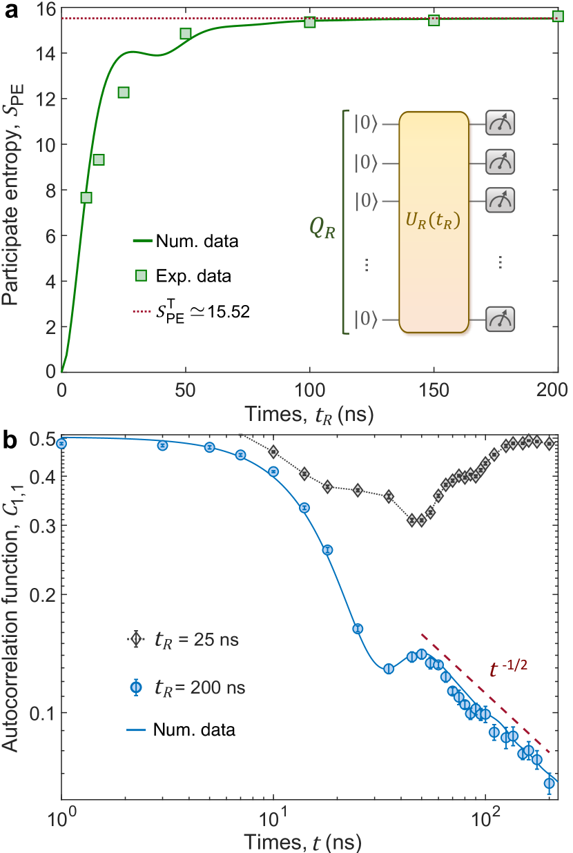
Figure 2: Observation of diffusive transport. a, Experimental verification of preparing the states via the time evolution of participate entropy. Here, we chose $Q_{R}=\{Q_{1,\uparrow},Q_{2,\uparrow},...,Q_{12,\uparrow},Q_{2,\downarrow},Q_{3,\downarrow},...,Q_{12,\downarrow}\}$ with total 23 qubits. The inset of a shows the corresponding quantum circuit. The dotted horizontal line represents the psedo-random value of participate entropy, i.e., $S_{\text{PE}}^{\text{T}}\simeq 15.519$. b, Experimental results of the autocorrelation function $C_{1,1}(t)$ for the qubit ladder with $L=12$, which are measured by performing the quantum circuit shown in Fig. 1c and d. Here, we consider two different states generated from $\hat{U}_{R}(t_{R})$ with $t_{R}=25$ ns and $200$ ns. Markers are experimental data. The solid line is the numerical simulation of the correlation function $C_{1,1}$ at infinite temperature. The dashed line represents a power-law decay $t^{-1/2}$. Error bars represent the standard deviation.

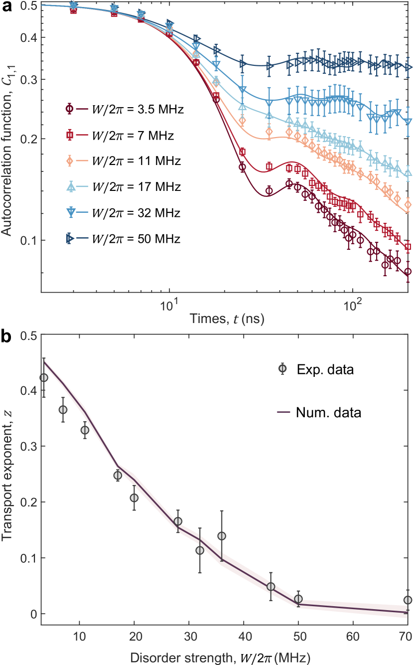
Figure 3: Subdiffusive transport on the superconducting qubit ladder with disorder. a, The time evolution of autocorrelation function $C_{1,1}(t)$ for the qubit ladder with $L=12$ and different values of disorder strength $W$. Markers (lines) are experimental (numerical) data. b, Transport exponent $z$ as a function of $W$ obtained from fitting the data of $C_{1,1}(t)$. Error bars (experimental data) and shaded regions (numerical data) represent the standard deviation.

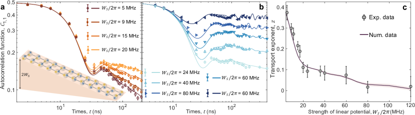
Figure 4: Subdiffusive transport on the superconducting qubit ladder with linear potential. a, Time evolution of autocorrelation function $C_{1,1}(t)$ for the disordered qubit ladder with $L=12$ and $W_{S}/2\pi\leq 20$ MHz. b is similar to a but for the data with $W_{S}/2\pi\geq 24$ MHz. Markers (lines) are experimental (numerical) data. c, Transport exponent $z$ as a function of $W_{S}$. For $W_{S}/2\pi\leq 20$ MHz and $W_{S}/2\pi\geq 24$ MHz, the exponent $z$ is extracted from fitting the data of $C_{1,1}(t)$ with the time window $t\in[50\text{ns},200\text{ns}]$ and $t\in[100\text{ns},400\text{ns}]$, respectively. Error bars (experimental data) and shaded regions (numerical data) represent the standard deviation.

In Fig. 2b, we show the dynamics of the autocorrelation function $C_{1,1}$ measured via the quantum circuit in Fig. 1c with $t_{R}=200$ ns. The experimental data satisfies $C_{1,1}\propto t^{-z}$, with a transport exponent $z\simeq 0.5067$, estimated by fitting the data in the time window $t\in[50\,\text{ns},200\,\text{ns}]$. In contrast, with $t_{R}=25$ ns, the state $|\psi^{R}\rangle$ does not approach to the Haar-random states, and its value of $S_{\text{PE}}$ is much smaller than the $S_{\text{PE}}^{\text{T}}$ (Fig. 2a). By employing the state $|\psi^{R}\rangle$ with $t_{R}=25$ ns, the values of the observable defined in Eq. (4) is incompatible with diffusive transport (Fig. 2b). Our experiments clearly show that spin diffusively transports on the qubit ladder $\hat{H}_{I}$ (1), and demonstrate that the analog pseudo-random quantum circuit $\hat{U}_{R}(t_{R})$ with $t_{R}=200$ ns can provide sufficient randomness to measure the autocorrelation function defined in Eq. (2) and probe infinite-temperature spin transport. In the following, we fix $t_{R}=200$ ns, and study spin transport in other systems with ergodicity breaking.

Subdiffusive transport with ergodicity breaking

After demonstrating that the quantum circuit shown in Fig. 1c can be employed to measure the infinite-temperature autocorrelation function $C_{1,1}$, we study spin transport on the superconducting qubit ladder with disorder, whose effective Hamiltonian can be written as $\hat{H}_{D}=\hat{H}_{I}+\sum_{m\in\{\uparrow,\downarrow\}}\sum_{j=1}^{L}w_{j,m}\hat{\sigma}_{j,m}^{+}\hat{\sigma}_{j,m}^{-}$, with $w_{j,m}$ drawn from a uniform distribution $[-W,W]$, and $W$ being the strength of disorder. The results of $C_{1,1}$ with different $W$ are plotted in Fig. 3a. With the increasing of $W$, and as the system approaches the MBL transition, $C_{1,1}$ decays more slowly. We then fit both the experimental and numerical data with the time window $t\in[50\,\text{ns},200\,\text{ns}]$ by adopting the power-law decay $C_{1,1}\propto t^{-z}$. As shown in Fig. 3b, we observe an anomalous subdiffusive region with the transport exponent $z<1/2$. For the strength of disorder $W/2\pi\gtrsim 50$ MHz, the transport exponent $z\sim 10^{-2}$, indicating the freezing of spin transport and the onset of MBL on the 24-qubit system Agarwal et al. (2015).

Next, we explore the transport properties on a titled superconducting qubit ladder, which is subjected to the linear potential $\hat{H}_{L}=\sum_{j=1}^{L}\gamma j\sum_{m\in\{\uparrow,\downarrow\}}\hat{\sigma}_{j,m}^{+}\hat{\sigma}_{j,m}^{-}$, with $\gamma=2W_{S}/(L-1)$ being the slope of the linear potential (see the titled ladder in the inset of Fig. 4a). Thus, the effective Hamiltonian of the titled superconducting qubit ladder can be written as $\hat{H}_{T}=\hat{H}_{I}+\hat{H}_{L}$. Different from the aforementioned breakdown of ergodicity induced by the disorder, the linear potential can also halt the onset of ergodic behaviors, resulting in the Stark MBL in disorder-free systems Guo et al. (2021b); Morong et al. (2021); Guo et al. (2021b); Schulz et al. (2019); van Nieuwenburg et al. (2019); Wang et al. (2021); Taylor et al. (2020).

We employ the method based on the quantum circuit shown in Fig. 1c to measure the time evolution of the autocorrelation function $C_{1,1}$ with different slopes of the linear potential. The results are presented in Fig. 4a and 4b. Similar to the system with disorder, the dynamics of $C_{1,1}$ still satisfies $C_{1,1}\propto t^{-z}$ with $z<0.5$, i.e., subdiffusive transport. Figure 4c displays the transport exponent $z$ with different strength of the linear potential, showing that $z$ asymptotically drops as $W_{S}$ increases. By employing the same standard for the onset of MBL induced by disorder, i.e., $z\sim 10^{-2}$, the results in Fig. 4c indicate that the Stark MBL on the titled 24-qubit ladder occurs when $W_{S}/2\pi\gtrsim 80$ MHz ($\gamma/2\pi\gtrsim 14.6$ MHz).

Discussion

Based on the novel protocol for simulating the infinite-temperature spin transport using the Haar-random state Richter and Pal (2021), we have experimentally probed diffusive transport on a 24-qubit ladder-type programmable superconducting processor. Moreover, when the qubit ladder is subject to sufficiently strong disorder or linear potential, we observe the signatures of subdiffusive transport, in accompany with the breakdown of ergodicity due to the conventional or Stark MBL.

Ensembles of Haar-random pure quantum states have several promising applications, including benchmarking quantum devices C. et al. (2023); Cross et al. (2019) and demonstrating the quantum advantage Neill et al. (2018); Boixo et al. (2018); Arute et al. (2019); Wu et al. (2021); Morvan et al. (2023). Our work displays a practical application of the randomly distributed quantum state, i.e., probing the infinite-temperature spin transport. In contrast to employing digital random circuits, where the number of imperfect two-qubit gates is proportional to the qubit number Boixo et al. (2018); Arute et al. (2019); Wu et al. (2021); Morvan et al. (2023); Richter and Pal (2021); Keenan et al. (2023), the scalable analog circuit adopted in our experiments can also generate multi-qubit Haar-random states useful for simulating hydrodynamics. The protocol employed in our work can be naturally extended to explore the non-trivial transport properties on other analog quantum simulators, including the Rydberg atoms Saffman et al. (2010); Browaeys and Lahaye (2020); Henriet et al. (2020), quantum gas microscopes Gross and Bloch (2017), and the waveguide or cavity QED setups Ballester et al. (2012); Xu et al. (2020, 2022); Zhang et al. (2023).

Methods

Derivation of Eq. (4)

Here, we present the details of the deviation of Eq. (4), which is based on the typicality Richter and Pal (2021); Schubert et al. (2021); Jin et al. (2020). According to Eq. (2), $c_{\alpha;\beta}=\text{Tr}[\hat{\sigma}_{\alpha}^{z}(t)\hat{\sigma}_{\beta}^{z}]/D$, with $D=2^{L}$. We define $\hat{N}_{\beta}=(\hat{\sigma}_{\beta}^{z}+1)/2$, and then $c_{\alpha;\beta}=\frac{2}{D}\text{Tr}[\hat{\sigma}_{\alpha}^{z}(t)\hat{N}_{\beta}]$. By using $\hat{N}_{\beta}=(\hat{N}_{\beta})^{2}$, we have $c_{\alpha;\beta}=\frac{2}{D}\text{Tr}[\hat{N}_{\beta}\hat{\sigma}_{\alpha}^{z}(t)\hat{N}_{\beta}]$.

According to the typicality Richter and Pal (2021); Schubert et al. (2021); Jin et al. (2020), the trace of an operator $\hat{O}$ can be approximated as the expectation value averaged by the pure Haar-random state $|r\rangle$, i.e.,

$$\frac{1}{D}\text{Tr}[\hat{O}]\simeq\langle r|\hat{O}|r\rangle.$$ (5)

Thus, $c_{\alpha;\beta}\simeq 2\langle r|\hat{N}_{\beta}\hat{\sigma}_{\alpha}^{z}(t)\hat{N}_{\beta}|r\rangle=\langle\psi_{\beta}^{R}(t)|\hat{\sigma}^{z}_{\alpha}|\psi_{\beta}^{R}(t)\rangle$.

Superconducting transmon qubit
A transmon qubit is composed of a capacitance $C$ and a nonlinear inductance $L$ (Josephson junction or SQUID). Its Lagrangian $\mathcal{L}_{0}$ and Hamiltonian $H_{0}$ can be written as

$$\mathcal{L}_{0} = \frac{Q^{2}}{2C}-\frac{\Phi^{2}}{2L}$$ (6)

$$H_{0} = \frac{Q^{2}}{2C}+\frac{\Phi^{2}}{2L},$$ (7)

where $Q=\partial\mathcal{L}_{0}/\partial{\dot{\Phi}}=C\dot{\Phi}$ denotes the charge, and $\Phi$ is the magnetic flux of the circuit. Here, the nonlinear inductance of the Josepshon junction with energy $E_{\text{J}}$ can be written as $L=L_{\text{c}}/{\cos{\left(2\pi{\Phi}/{\Phi_{0}}\right)}}$, where $\Phi_{0}=\hbar\pi/\mathrm{e}$ is the superconducting flux quantum, $\mathrm{e}\approx 1.602\times 10^{-19}$C is the electron charge, and $L_{\text{c}}=\Phi_{0}^{2}/(4\pi^{2}E_{\mathrm{J}})$ is the constant inductance. This nonlinear inductance can be easily derived from the definition $L=\mathrm{d}\Phi/\mathrm{d}I$ and the Josephson equation $I=I_{\text{c}}\sin{(2\pi{\Phi}/{\Phi_{0}})}$ with $I_{\text{c}}=2\pi{E_{\mathrm{J}}}/\Phi_{0}$ being the Josephson critical current.

Considering the weak flux $\Phi$, one can use the approximation $\cos{(2\pi{\Phi}/{\Phi_{0}})}\simeq{1-(2\pi{\Phi}/{\Phi_{0}})^{2}/2}$ and reduce the Hamiltonian Eq. (7) into $H_{0}\simeq\frac{Q^{2}}{2C}+\frac{\Phi^{2}}{2L_{\text{c}}}-\frac{\pi^{2}\Phi^{4}}{4L_{\text{c}}\Phi_{0}^{2}}$, which can be viewed as a harmonic oscillator with $o(\Phi^{4})$ perturbation. Using canonical quantization, one can introduce

$$\begin{cases}&\!\!\!\!\hat{Q}=\mathrm{i}Q_{\text{zpf}}(\hat{a}^{\dagger}-\hat{a})\cr&\!\!\!\!\hat{\Phi}=\Phi_{\text{zpf}}(\hat{a}^{\dagger}+\hat{a})\end{cases}$$ (8)

with $Q_{\text{zpf}}=\sqrt{\hbar(C/L_{\text{c}})^{\frac{1}{2}}/2}$ and $\Phi_{\text{zpf}}=\sqrt{\hbar(L_{\text{c}}/C)^{\frac{1}{2}}/2}$ being the zero point fluctuation of the charge and flux operators, respectively. The quantized Hamiltonian thus is (the constant term is omitted):

$$\hat{H}_{0}=\hbar\omega\hat{a}^{\dagger}\hat{a}-\frac{E_{\mathrm{C}}}{2}\hat{a}^{\dagger}\hat{a}^{\dagger}\hat{a}\hat{a},$$ (9)

where $\omega=(\sqrt{8E_{\mathrm{C}}E_{\mathrm{J}}}-E_{\mathrm{C}})/\hbar$ denotes the qubit frequency, and $E_{\mathrm{C}}=\mathrm{e}^{2}/(2C)$ is the charging energy that represents the magnitude of anharmonicity. For a single Josephson junction, $E_{\mathrm{J}}$ is not tunable, while for a SQUID with two junctions, it depends on the external flux $\Phi_{\text{ext}}$ applied to the junction region. In the experiments, we can adjust the qubit frequency $\omega$ via the external fast flux bias applied to the Z control line.

XY drive in superconducting circuits
When a time-dependent driving voltage $V_{\text{d}}(t)$ is added to XY line of the qubit, the total Lagrangian is given by

$$\mathcal{L}_{\text{driven}}=\frac{1}{2}C\dot{\Phi}^{2}+\frac{1}{2}C_{\text{d}}\left(V_{\text{d}}(t)-\dot{\Phi}\right)^{2}-\frac{\Phi^{2}}{2L},$$ (10)

where $C_{\text{d}}$ is the driving capacitance. The Lagrangian $\mathcal{L}_{\text{driven}}$ can be verified by the Kirchhoff laws for this driven system.

To obtain the Hamiltonian, we first calculate the conjugate to the position (flux) $\Phi$, namely the canonical momentum (charge) $\tilde{Q}={\partial\mathcal{L}_{\text{driven}}}/{\partial\dot{\Phi}}=C_{\Sigma}\dot{\Phi}-C_{\text{d}}V_{\text{d}}(t)$, and thus

$$H_{\text{driven}}=\tilde{Q}\dot{\Phi}-\mathcal{L}_{\text{driven}}=\frac{\tilde{Q}}{2C_{\Sigma}}+\frac{\Phi^{2}}{2L}+\frac{\tilde{Q}C_{\text{d}}V_{\text{d}}(t)}{C_{\Sigma}}.$$ (11)

Using the canonical quantization procedure like Eq. (8), we introduce $\hat{\tilde{Q}}=\text{i}\tilde{Q}_{\text{zpf}}(\hat{a}^{\dagger}-\hat{a})$ and $\hat{\Phi}=\Phi_{\text{zpf}}(\hat{a}^{\dagger}+\hat{a})$ to quantize the driven system, where $\tilde{Q}_{\text{zpf}}=\sqrt{\hbar(C_{\Sigma}/L_{\text{c}})^{\frac{1}{2}}/2}$ and $\Phi_{\text{zpf}}=\sqrt{\hbar(L_{\text{c}}/C_{\Sigma})^{\frac{1}{2}}/2}$. Hence, the Hamiltonian becomes

$$~{}\hat{H}_{\text{driven}}=\hbar\omega\hat{a}^{\dagger}\hat{a}-\frac{E_{\mathrm{C}}}{2}\hat{a}^{\dagger}\hat{a}^{\dagger}\hat{a}\hat{a}+\mathrm{i}\hbar\Omega(t)(\hat{a}^{\dagger}-\hat{a}),$$ (12)

where $E_{\text{C}}=\mathrm{e}^{2}/(2C_{\Sigma})$, $E_{\mathrm{J}}={\Phi_{0}^{2}}/{4\pi^{2}L_{\text{c}}}$, $\omega=\sqrt{8E_{\mathrm{C}}E_{\mathrm{J}}}-E_{\mathrm{C}}$, $\Omega(t)=\epsilon V_{\text{d}}(t)$, $\epsilon={\tilde{Q}_{\text{zpf}}C_{\text{d}}}/{(\hbar C_{\Sigma})}$. Here, we set the time-dependent driving $V_{\text{d}}(t)=-V_{\text{d}}\sin\left(\omega_{\text{d}}t+\phi\right)=\mathrm{Im}\{V_{\text{d}}e^{-\mathrm{i}(\omega_{\text{d}}t+\phi)}\}$, thus $\Omega(t)=\mathrm{i}\Omega\left(e^{-\mathrm{i}(\omega_{\text{d}}t+\phi)}-e^{\mathrm{i}(\omega_{\text{d}}t+\phi)}\right)/2$, where $\Omega=\epsilon V_{\text{d}}$ is so-called Rabi frequency. The parameter $\epsilon$ represents the Rabi frequency corresponding to the unit amplitude of the drive.

To solve the time evolution governed by the above time-dependent Hamiltonian, we consider the rotating frame which is generated by $\hat{U}_{d}(t)=e^{\mathrm{i}\omega_{\text{d}}t\hat{a}^{\dagger}\hat{a}}$

$$\hat{H}_{d} = \hat{U}_{d}(t)\hat{H}_{\text{driven}}(t)\hat{U}^{\dagger}_{d}(t)+\mathrm{i}\hbar\left(\frac{\mathrm{d}}{\mathrm{d}t}\hat{U}_{d}(t)\right)\hat{U}^{\dagger}_{d}(t)$$ (13)

$$\simeq \hbar\Delta\hat{a}^{\dagger}\hat{a}-\frac{E_{\mathrm{C}}}{2}\hat{a}^{\dagger}\hat{a}^{\dagger}\hat{a}\hat{a}+\frac{\hbar\Omega}{2}\!\left(\hat{a}^{\dagger}e^{-\mathrm{i}\phi}\!+\!\hat{a}e^{\mathrm{i}\phi}\right),$$

where $\Delta=\omega-\omega_{\text{d}}$ is the frequency detuning, and the rotating-wave approximation is adopted by ignoring high frequency oscillation $\pm 2\omega_{\text{d}}$.

With $\Delta=0$ and $E_{\mathrm{C}}\gg\Omega$, the large anharmonicity results in the resonant drive acting almost exclusively between the first two energy levels $\ket{0}$ and $\ket{1}$ without leakage to higher levels. Hence, considering the two-level qubit, we have

$$\hat{H}_{d}=\frac{\hbar\Omega}{2}\left(\hat{\sigma}^{+}e^{-\mathrm{i}\phi}+\hat{\sigma}^{-}e^{\mathrm{i}\phi}\right),$$ (14)

where $\hat{\sigma}^{+}_{j}$ ($\hat{\sigma}^{-}_{j}$) is the raising (lowering) operator. If the qubit begins in the ground state $\ket{0}$, its time-dependent state during the unitary evolution is

$$\ket{\psi_{d}(t)}=e^{-\frac{\mathrm{i}}{\hbar}\hat{H}_{d}t}\ket{0}=\cos{\frac{\Omega t}{2}}\ket{0}-\mathrm{i}e^{\mathrm{i}\phi}\sin{\frac{\Omega t}{2}}\ket{1},$$ (15)

and the probability of qubit in $\ket{1}$ is given by $P_{1}(t)=\sin^{2}{({\Omega t}/{2})}=\left[1-\cos{\left(\Omega t\right)}\right]/2$. Considering the energy relaxation, the envelope of $P_{1}(t)$ will decay in a dissipative evolution and thus

$$~{}P_{1}(t)=\frac{1}{2}\left[1-e^{-\frac{t}{T_{1}}}\cos{\left(\Omega t\right)}\right],$$ (16)

where $T_{1}$ is the energy relaxation time that depends on the qubit frequency $\omega$. In order to obtain the Rabi frequency $\Omega$, one can fit the data of $P_{1}(t)$ by using the form of function $A\exp{(-{t}/{T_{1}})}\cos{\left(\Omega t\right)}+B$. Typical experimental data of calibrating XY drive with different driving amplitudes are displayed in Extended Data Fig. 1.

The above results are based on the resonance condition $\omega=\omega_{\text{d}}$. If the detuning $\Delta=\omega-\omega_{\text{d}}\neq 0$, the effective Rabi frequency will be $\Omega_{\text{R}}=\sqrt{\Delta^{2}+\Omega^{2}}$. Therefore, to obtain the correct Rabi frequency when $\omega=\omega_{\text{d}}$, we should find the corresponding Z pulse amplitude that makes the qubit resonate with the microwave before calibrating XY drive. This step can be easily achieved via spectroscopy experiment or Rabi oscillation by scanning the Z pulse amplitude of the qubit.

Microwave crosstalk and correction
Consider two driven qubits $Q_{i}$ and $Q_{j}$ coupled by a coupling capacitance $C_{ij}$, the quantized Hamiltonian is (see Supplementary Section IV)

$$\hat{H}^{(i,j)}_{\text{driven}} = \hat{H}^{(i)}_{\text{driven}}+\hat{H}^{(j)}_{\text{driven}}+\hat{H}^{(i,j)}_{\text{int}},$$ (17)

$$\hat{H}^{(q)}_{\text{driven}} = \hbar\omega_{q}\hat{a}^{\dagger}_{q}\hat{a}_{q}-\frac{E_{\mathrm{C}_{q}}}{2}\hat{a}^{\dagger}_{q}\hat{a}_{q}^{\dagger}\hat{a}_{q}\hat{a}_{q}$$ (18)

$$+~{}\!\mathrm{i}\hbar\tilde{\Omega}_{q}(t)(\hat{a}^{\dagger}_{q}-\hat{a}_{q}),\quad q\in{\{i,j\}},$$

$$\hat{H}^{(i,j)}_{\text{int}} = \hbar{J_{i,j}}(\hat{a}^{\dagger}_{i}-\hat{a}_{i})(\hat{a}_{j}-\hat{a}^{\dagger}_{j}),$$ (19)

where $J_{ij}$ is the coupling strength and

$$\!\!\!\!\!\!\!\!\!\!\tilde{\Omega}_{i}(t)=\epsilon_{ii}\left(V_{\text{d},i}(t)+\frac{\epsilon_{ij}}{\epsilon_{ii}}V_{\text{d},j}(t)\right),$$ (20)

$$\!\!\!\!\!\!\!\!\!\!\tilde{\Omega}_{j}(t)=\epsilon_{jj}\left(V_{\text{d},j}(t)+\frac{\epsilon_{ji}}{\epsilon_{jj}}V_{\text{d},i}(t)\right).$$ (21)

The parameters $\epsilon_{ij}$ and $\epsilon_{ji}$ are explained in Supplementary Section IV, which depends on the coupling capacitance $C_{ij}$ between the two qubits. Here, we focus on the origin of the crosstalk. Given the above equations, we note that the local driving Hamiltonian of each qubit is subject to both external drive $V_{\text{d},i}(t)$ and $V_{\text{d},j}(t)$ due to the presence of coupling capacitance. However, this crosstalk is usually very small. In fact, most of the crosstalk comes from the classical microwave crosstalk. The total crosstalk is the sum of the classical microwave crosstalk and the crosstalk due to the coupling capacitance. In the following, we will establish a model to describe the total crosstalk and introduce an efficient method for measuring the crosstalk matrix.

When the microwave signal travels through the medium on the chip, it can be described by the plane wave form $V_{\text{d}}(\mathbf{r},t)=V_{\text{d}}(t)e^{\mathrm{i}\mathbf{k}\cdot\mathbf{r}}.$ Here, the wave vector $\mathbf{k}$ is generally complex, namely $\mathbf{k}=\mathbf{b}+\mathrm{i}\mathbf{a}$, thus we have $\mathrm{i}\mathbf{k}\cdot\mathbf{r}=-\mathbf{a}\cdot\mathbf{r}+\mathrm{i}\mathbf{b}\cdot\mathbf{r}$, where the first term is the amplitude attenuation induced by the imaginary part of $\mathbf{k}$ and the second term is the phase retardation caused by the real part.

As shown in Extended Data Fig. 2, the signal $V_{\text{d},i}(t)$ propagates from $Q_{i}$ to $Q_{j}$ with a factor $e^{-\xi_{ji}+\mathrm{i}\phi_{ji}}$ attached, which implies the classical microwave crosstalk of $Q_{i}$ to $Q_{j}$. Similarly, the classical microwave crosstalk of $Q_{j}$ to $Q_{i}$ can be express as $V_{\text{d},j}(t)e^{-\xi_{ij}+\mathrm{i}\phi_{ij}}$. Moreover, the crosstalk caused by the coupling capacitance is also considered. Therefore, the total signals perceived by $Q_{i}$ and $Q_{j}$ are

$$\begin{bmatrix}\tilde{V}_{\text{d},i}(t)\\ \tilde{V}_{\text{d},j}(t)\end{bmatrix}=\begin{bmatrix}1&{v_{ij}}e^{\mathrm{i}\varphi_{ij}}\\ {v_{ji}}e^{\mathrm{i}\varphi_{ji}}&1\end{bmatrix}\begin{bmatrix}V_{\text{d},i}(t)\\ V_{\text{d},j}(t)\end{bmatrix}$$ (22)

with the definitions of ${v_{ij}}e^{\mathrm{i}\varphi_{ij}}={\epsilon_{ij}}/{\epsilon_{ii}}+e^{-\xi_{ij}+\mathrm{i}\phi_{ij}}$ and ${v_{ji}}e^{\mathrm{i}\varphi_{ji}}={\epsilon_{ji}}/{\epsilon_{jj}}+e^{-\xi_{ji}+\mathrm{i}\phi_{ji}}$. To generalize the above formula to the case of each qubit with crosstalks from all other qubits, we define the vectors $\mathbf{\tilde{V}_{\!d}}(t)=[\tilde{V}_{\text{d},1}(t),\tilde{V}_{\text{d},2}(t),\ldots,~{}\!\tilde{V}_{\text{d},N}(t)]^{T}$ and $\mathbf{V_{\!d}}(t)=[V_{\text{d},1}(t),V_{\text{d},2}(t),\dots,~{}\!V_{\text{d},N}(t)]^{T}$, then

$$\mathbf{\tilde{V}_{\!d}}(t)=\mathbf{M_{V}}\mathbf{V_{\!d}}(t),$$ (23)

in which $\mathbf{M_{V}}$ is the signal crosstalk matrix

$$\mathbf{M_{V}}=\begin{bmatrix}1&{v_{12}}e^{\mathrm{i}\varphi_{12}}&\cdots&{v_{1N}}e^{\mathrm{i}\varphi_{1N}}\\ {v_{21}}e^{\mathrm{i}\varphi_{21}}&1&\cdots&{v_{2N}}e^{\mathrm{i}\varphi_{2N}}\\ \vdots&\vdots&\ddots&\vdots\\ {v_{N1}}e^{\mathrm{i}\varphi_{N1}}&{v_{N2}}e^{\mathrm{i}\varphi_{N2}}&\cdots&1\end{bmatrix}.$$ (24)

To correct the crosstalk, one can measure the total signal crosstalk matrix and perform

$$\mathbf{V_{\!d}}(t)=\mathbf{M^{-1}_{V}}~{}\!\mathbf{\tilde{V}_{\!d}}(t),$$ (25)

where $\mathbf{M^{-1}_{V}}$ is the inverse matrix. However, in practice, the matrix $\mathbf{M_{V}}$ cannot be directly measured. Thus, we need to measure the crosstalk matrix of Rabi frequencies $\mathbf{M_{\Omega}}$ and calculate $\mathbf{M_{V}}$ by using

$$\mathbf{M_{V}}=\bm{\epsilon}~{}\!\mathbf{M_{\Omega}}~{}\!\bm{\epsilon^{-1}},$$ (26)

where $\bm{\epsilon}=\mathrm{diag}\{\epsilon_{11},\epsilon_{22},\ldots,~{}\!\epsilon_{NN}\}$, and the crosstalk matrix of Rabi frequencies is defined as

$$\mathbf{M_{\Omega}}=\begin{bmatrix}1&{c_{12}}e^{\mathrm{i}\varphi_{12}}&\cdots&{c_{1N}}e^{\mathrm{i}\varphi_{1N}}\\ {c_{21}}e^{\mathrm{i}\varphi_{21}}&1&\cdots&{c_{2N}}e^{\mathrm{i}\varphi_{2N}}\\ \vdots&\vdots&\ddots&\vdots\\ {c_{N1}}e^{\mathrm{i}\varphi_{N1}}&{c_{N2}}e^{\mathrm{i}\varphi_{N2}}&\cdots&1\end{bmatrix}.$$ (27)

Here, $c_{ij}$ and $\varphi_{ij}$ are the amplitude and phase crosstalk coefficients to be measured.

Measurement of crosstalk matrix
Now, we introduce an efficient method for measuring the crosstalk matrix. Let us take an example of $Q_{i}$. As shown in Extended Data Fig. 3a, two resonant microwave signals $\omega_{\text{d},i}=\omega_{\text{d},j}=\omega_{\text{d}}$ are simultaneously input from the XY control lines of $Q_{i}$ and $Q_{j}$. Meanwhile, $Q_{i}$ is biased near the resonant frequency with the detuning $\Delta_{i}=\omega_{i}-\omega_{\text{d},i}$. Due to the crosstalk, the effective Hamiltonian of $Q_{i}$ under the rotation frame becomes $\hat{H}_{d}^{(i)}=\Delta_{i}\hat{\sigma}^{+}_{i}\hat{\sigma}^{-}_{i}+\left(\tilde{\Omega}_{i}\hat{\sigma}^{+}_{i}+\mathrm{H.c.}\right)/{2}$ with $\tilde{\Omega}_{i}=\Omega_{i}e^{-\mathrm{i}\phi_{i}}+c_{ij}\Omega_{j}e^{\mathrm{i}(\varphi_{ij}-\phi_{j})}$, and the corresponding effective Rabi frequency is

$$\Omega_{\text{R}}^{(i)}=\sqrt{\Delta_{i}^{2}+\Omega_{i}^{2}+\Omega_{ij}^{2}+2\Omega_{i}\Omega_{ij}\cos{(\varphi_{ij}-\varphi_{ii})}},$$ (28)

where $\Omega_{ij}=c_{ij}\Omega_{j}$ denotes the crosstalk Rabi frequency from $Q_{j}$ to $Q_{i}$, and $\varphi_{ii}=\phi_{j}-\phi_{i}$ represents the additional XY phase added in $Q_{i}$ relative to $Q_{j}$. By scanning $\varphi_{ii}$ and measure the probabilities of $Q_{i}$ in $\ket{1}$ as a function of the duration of XY drive, we can obtain $\Omega_{\text{R}}^{(i)}$. Using Eq. (28) to fit the results of $\Omega_{R}^{(i)}$, we can determine the crosstalk coefficients $c_{ij}$ and $\varphi_{ij}$. The procedure for determining $c_{ji}$ and $\varphi_{ji}$ is similar as long as we treat $Q_{j}$ as $Q_{i}$.

Numerical simulations
Here, we present the details of the numerical simulations. We calculate the unitary time evolution $|\psi(t+\Delta t)\rangle=e^{-i\hat{H}\Delta t}|\psi(t)\rangle$ by employing the Krylov method Luitz and Lev (2017). The Krylov subspace is panned by the vectors defined as $\{|\psi(t)\rangle,\hat{H}|\psi(t)\rangle,\hat{H}^{2}|\psi(t)\rangle,...,\hat{H}^{(m-1)}|\psi(t)\rangle\}$. Then, the Hamiltonian $\hat{H}$ in the Krylov subspace becomes a $m$-dimensional matrix $\text{H}_{m}=\text{K}_{m}^{\dagger}\text{H}\text{K}_{m}$, where H denotes the Hamiltonian $\hat{H}$ in the matrix form, and $\text{K}_{m}$ is the matrix whose columns contain the orthonormal basis vectors of the Krylov space. Finally, the unitary time evolution can be approximately simulated in the Krylov subspace as $|\psi(t+\Delta t)\rangle\simeq\text{K}_{m}^{\dagger}e^{-i\text{H}_{m}\Delta t}\text{K}_{m}|\psi(t)\rangle$. In our numerical simulations, the dimension of the Krylov subspace $m$ is adaptively adjusted from $m=6$ to $30$, making sure the numerically errors are smaller than $10^{-14}$.

For the numerical simulation of the $\hat{U}_{R}(t_{R})=e^{-i\hat{H}_{d}t_{R}}$ in Fig. 1c, based on the experimental data of the XY drive, the parameters in $\hat{H}_{d}$ are $\Omega_{j,m}/2\pi=10.4\pm 1.6$ MHz, and $\phi_{j,m}\in[-\pi/10,\pi/10]$.

Data availability
All data needed to evaluate the conclusions in the paper are present in the paper and/or the Supplementary Information.

Acknowledgments
We thank Hai-Long Shi and H. S. Yan for helpful discussions. This work was supported by National Natural Science Foundation of China (Grants Nos. 11934018, 92265207, T2121001, 12122504, 12247168), Beijing Natural Science Foundation (Grant No. Z200009), Innovation Program for Quantum Science and Technology (Grant No. 2021ZD0301800), Beijing Nova Program (No. 20220484121), Scientific Instrument Developing Project of Chinese Academy of Sciences (Grant No. YJKYYQ20200041), and China Postdoctoral Science Foundation (Certificate Number: 2022TQ0036).

Author contributions
H.F. supervised the project. Z.-H.S. proposed the idea. Y.-H.S. conducted the experiment with the help of K.H. and K.X.. Z.-H.S., Y.-Y.W., and Y.-H.S. performed the numerical simulations. Z.X. and D.Z. fabricated the ladder-type sample. X.S., G.X., and H.Y. provided the Josephson parametric amplifiers. W.-G.M., H.-T.L., K.Z., J.-C.S., G.-H.L., Z.-Y.M., J.-C.Z., H.L., and C.-T.C. helped the experimental setup. Z.-A.W., Y.-R.Z., J.W., K.X., and H.F. discussed and commented on the manuscript. Z.-H.S., Y.-H.S., Y.-Y.W., Y.-R.Z., and H.F. co-wrote the manuscript. All authors contributed to the discussions of the results and development of the manuscript.

Competing interests
The authors declare no competing interests.

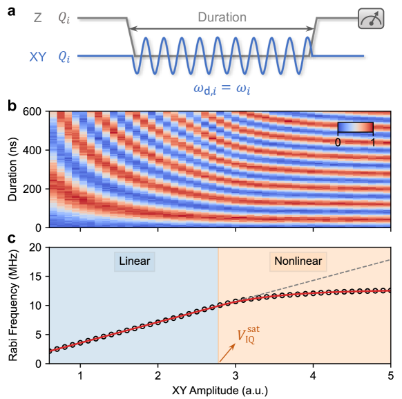
Extended data Fig. 1: Typical experimental data of measuring the relationship between Rabi frequency and XY drive amplitude. a, Experimental pulse sequence. Qubit is detuned from its idle frequency to the operating $\omega_{i}$. Meanwhile, we apply resonant microwave drives on this qubit with scanning XY amplitude $V_{\text{IQ}}$ and measure the vacuum Rabi oscillations shown in b. b, The heatmap of the probabilities of qubit in the state $\ket{1}$ as a function of duration and XY amplitude. c, For each XY drive amplitude, we fit the curve of vacuum Rabi oscillation by using Eq. (16) to obtain the experimental Rabi frequency, denoted as black hollow circle. The red solid line is the result of fitting the experimental Rabi frequencies by using a smooth piecewise function and the grey dashed line implies the linear relationship between Rabi frequency and XY drive amplitude when the drive amplitude is less than $V^{\text{sat}}_{\text{IQ}}$.

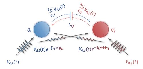
Extended data Fig. 2: Schematic of microwave signal crosstalk. Here, we take two qubits $Q_{i}$ and $Q_{j}$ as an example. Their individual driving voltages $V_{\mathrm{d},i}(t)$ and $V_{\mathrm{d},j}(t)$ induce two types of crosstalk. One type of crosstalk is due to the presence of coupling capacitance $C_{ij}$, which causes the crosstalk only in amplitude. The parameters $\epsilon_{ij}$ and $\epsilon_{ji}$ are explained in Supplementary Section IV, which depends on the coupling capacitance $C_{ij}$ between the two qubits. The other type of crosstalk is caused by the propagation of microwave signals through the medium on the chip. According to electrodynamics, it will lead to the crosstalk both in amplitude and phase. The parameters $\xi$ and $\phi$ are the amplitude attenuation factor and phase retardation of microwave propagation, respectively.

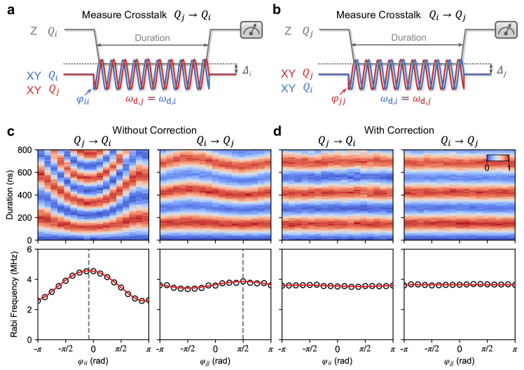
Extended data Fig. 3: Measurement of the microwave crosstalk. a, Experimental pulse sequence for measuring the crosstalk from $Q_{j}$ to $Q_{i}$. b, Experimental pulse sequence for measuring the crosstalk from $Q_{i}$ to $Q_{j}$. The parameters $\varphi_{ii}$ and $\varphi_{jj}$ denote the additional phases added into the XY control lines of $Q_{i}$ and $Q_{j}$, respectively. The detuning between the qubit frequency and XY drive frequency is defined as $\Delta_{q}=\omega_{q}-\omega_{\text{d},q}$, which is usually set to zero. c, Typical experimental data of measuring crosstalk without correction. d, Typical experimental data of measuring crosstalk with correction. The heatmap represents the probabilities of qubit in $\ket{1}$. The black hollow circle denotes the effective Rabi frequency obtained by fitting the Rabi oscillation. The red solid line is the result of fitting the effective Rabi frequency by using Eq. (28). The grey dashed line implies the fitted crosstalk phase.