The Mahler measure of exact polynomials in three variables

Abstract.

We prove that under certain explicit conditions, the Mahler measure of a three-variable exact polynomial can be expressed in terms of elliptic curve $L$-values and values of the Bloch-Wigner dilogarithm, conditionally on Beilinson's conjecture. In some cases, these dilogarithmic values simplify to Dirichlet $L$-values. This generalizes a result of Lalín [Lal15] for the polynomial $z+(x+1)(y+1)$. We apply our method to several other Mahler measure identities conjectured by Boyd and Brunault.

Introduction

Let $P(x_{1},\dots,x_{n})\in\mathbb{C}[x_{1}^{\pm 1},\dots,x_{n}^{\pm 1}]$ be a nonzero Laurent polynomial. The (logarithmic) Mahler measure of $P$ is defined by

(0.0.1) $$\mathrm{m}(P) =\dfrac{1}{(2\pi i)^{n}}\int_{\mathbb{T}^{n}}\log|P(x_{1},\dots,x_{n})|\ \dfrac{dx_{1}}{x_{1}}\wedge\cdots\wedge\dfrac{dx_{n}}{x_{n}},$$

where $\mathbb{T}^{n}:|x_{1}|=\dots=|x_{n}|=1$ is the $n$-dimensional torus. This quantity was firstly introduced by Mahler [Mah] in 1962.

In 1997, Deninger [Den97] linked the Mahler measure of polynomials $P(x_{1},\dots,x_{n})$ under certain conditions to the motivic cohomology of $V_{P}$, where $V_{P}$ is the zero locus of $P$ in $\mathbb{C}^{n}$. This allowed him to place the Mahler measure in the very general framework of Beilinson's conjectures on special values of $L$-functions. More precisely, Deninger defined the following chain

$$\Gamma=\{(x_{1},\dots,x_{n})\in\mathbb{C}^{n}:P(x_{1},\dots,x_{n})=0,|x_{1}|=\dots=|x_{n-1}|=1,|x_{n}|\geq 1\}.$$

He showed that if $\Gamma$ is contained in the regular locus $V_{P}^{\mathrm{reg}}$ of $V_{P}$, then there is a differential $(n-1)$-form $\eta(x_{1},\dots,x_{n})$ on $\mathbb{G}_{m}^{n}$ such that its restriction to $V_{P}$ represents the regulator of the Milnor symbol $\{x_{1},\dots,x_{n}\}$, and we have

(0.0.2) $$\mathrm{m}(P)=\mathrm{m}(\tilde{P})+\dfrac{(-1)^{n}}{(2\pi i)^{n-1}}\int_{\Gamma}\eta(x_{1},\dots,x_{n}),$$

where $\tilde{P}$ is the leading coefficient of $P$ seen as a polynomial in $x_{n}$.

From now on we assume that $P$ has rational coefficients and $\Gamma$ is contained in $V_{P}^{\mathrm{reg}}$. If $\partial\Gamma=\emptyset$, then $\Gamma$ is a cycle. Then Deninger found out that in certain situations, the identity (0.0.2) together with Beilinson's conjecture imply that $\mathrm{m}(P)$ can be expressed in terms of the $L$-function of the motive $H^{n-1}(\overline{V_{P}})$, where $\overline{V_{P}}$ is a smooth compactification of $V_{P}$. As an example, he showed that under the Beilinson conjecture,

(0.0.3) $$\mathrm{m}\left(x+\dfrac{1}{x}+y+\dfrac{1}{y}+1\right)\stackrel{{\scriptstyle?}}{{=}}L^{\prime}(E_{15},0),$$

where $E_{15}$ is the elliptic curve (of conductor 15) defined by $x+1/x+y+1/y+1=0$. In this example, $\partial\Gamma\neq\emptyset$ but a symmetry argument reduces this to the case $\partial\Gamma=\emptyset$. It was completely shown (without assuming the Beilinson conjecture) by Rogers and Zudilin [RZ] in 2014.

Boyd [Boy98] conjectured, based on numerical evidence, that

(0.0.4) $$\mathrm{m}\left(x+\dfrac{1}{x}+y+\dfrac{1}{y}+k\right)\stackrel{{\scriptstyle?}}{{=}}r_{k}\ L^{\prime}(E_{N(k)},0),$$

where $k\in\mathbb{Z}\setminus\{0,\pm 4\}$, $r_{k}\in\mathbb{Q}^{\times}$ and $E_{N(k)}$ is the elliptic curve (of conductor $N(k)$) obtained as a smooth compactification of the zero set of $P_{k}=x+1/x+y+1/y+k$. Until now, the identity (0.0.4) is only proved for a finite number of $k$:

$$k\in\{-4\sqrt{2},-2\sqrt{2},1,2,3,2\sqrt{2},3\sqrt{2},5,8,12,16,i,2i,3i,4i,\sqrt{2}i\},$$

by the works of Brunault, Lalín, Rodriguez-Villegas, Rogers, Samart, and Zudilin (see [Bru16], [Lal10], [LSZ], [LR], [Rod], [RZ]).

The case $\partial\Gamma\neq\emptyset$ is more difficult, Maillot [Mai] suggested we should look at the variety $W_{P}:=V_{P}\cap V_{P^{*}}$, where $P^{*}(x_{1},\dots,x_{n})=\bar{P}(x_{1}^{-1},\dots,x_{n}^{-1})$. If $P$ is an exact polynomial, i.e., $\eta=d\omega$, where $\omega$ is a differential form on $V_{P}^{\mathrm{reg}}$, then Stokes' theorem gives

$$\mathrm{m}(P)=\mathrm{m}(\tilde{P})+\dfrac{(-1)^{n-1}}{(2\pi i)^{n-1}}\int_{\partial\Gamma}\omega.$$

Moreover, $\partial\Gamma$ is contained in $W_{P}$, hence we can hope that $\mathrm{m}(P)$ is related to the cohomology of $W_{P}$. In this direction, Lalín [Lal15] showed the following result. Assume that $P\in\mathbb{Q}[x,y,z]$ is irreducible and satisfies the following conditions:

1. $W_{P}$ is birationally equivalent to an elliptic curve $E$ over $\mathbb{Q}$,

2. $\partial\Gamma$ defines an element of $H_{1}(E(\mathbb{C}),\mathbb{Z})^{+}$, the invariant part of $H_{1}(E(\mathbb{C}),\mathbb{Z})$ under the complex conjugation on $E(\mathbb{C})$,

3. $x\wedge y\wedge z=\sum_{j}f_{j}\wedge(1-f_{j})\wedge g_{j}\text{ in }\bigwedge^{3}\mathbb{Q}(V_{P})^{\times}$, for some functions $f_{j},g_{j}$ on $V_{P}$,

4. $x\wedge y\wedge z=0\text{ in }\bigwedge^{3}\mathbb{Q}(E)^{\times}$,

5. $\sum_{j}v_{p}(g_{j})\{f_{j}(p)\}_{2}=0\text{ in }\mathbb{Z}[\mathbb{P}^{1}_{\bar{\mathbb{Q}}}]/R_{2}(\bar{\mathbb{Q}})\text{ for all }p\in E(\bar{\mathbb{Q}})$,

where $R_{2}(\bar{\mathbb{Q}})$ is the subgroup generated by the five-term relations (cf. Equation (2.1.2)), and $v_{p}(g_{j})$ is the vanishing order at $p$ of $g_{j}$ seen as a function on $E$. Then under Beilinson's conjecture, M. Lalín showed

(0.0.5) $$\mathrm{m}(P)=m(\tilde{P})+a\cdot L^{\prime}(E,-1),\ a\in\mathbb{Q}.$$

Note that the condition (3) implies that $P$ is exact (see Example 4.3).

In this article, we relax Lalín's conditions in order to deal with Mahler measure identities which are more general than (0.0.5), for example, containing also Dirichlet $L$-values. We only assume that $W_{P}$ is of genus 1 and we do not require the conditions (4)-(5) above. Recall [Zag, § 2] that the Bloch-Wigner dilogarithm function $D:\mathbb{P}^{1}(\mathbb{C})\to\mathbb{R}$ is defined by

(0.0.6) $$D(z)=\begin{cases}\mathrm{Im}\left(\sum_{k=1}^{\infty}\frac{z^{k}}{k^{2}}\right)+\arg(1-z)\log|z|&(|z|\leq 1),\\ -D(1/z)&(|z|\geq 1).\end{cases}$$

For any field $F$, we denote by $B(F)$ the Bloch group of $F$ tensored with $\mathbb{Q}$ (see [Zag, §2]). Let $\tau$ be the involution of $\mathbb{G}^{3}_{m}$ given by $(x,y,z)\mapsto(1/x,1/y,1/z)$. Since $P$ has rational coefficients, $\tau$ induces an involution of $W_{P}$. For $A$ is a abelian group, we denote by $A_{\mathbb{Q}}:=A\otimes\mathbb{Q}$. Let us state our main theorem here.

Theorem 0.1.

Assume $P\in\mathbb{Q}[x,y,z]$ is irreducible and that $W_{P}$ is a curve of genus 1. Let $C$ be the normalization of $W_{P}$. Suppose that

(0.0.7) $$x\wedge y\wedge z=\sum_{j}f_{j}\wedge(1-f_{j})\wedge g_{j}\text{ in }\bigwedge^{3}\mathbb{Q}(V_{P})^{\times}_{\mathbb{Q}},$$

for some functions $f_{j},g_{j}$ on $V_{P}$. Let $S$ be the closed subscheme of $C$ consisting of the zeros and poles of the functions $g_{j}$ and $g_{j}\circ\tau$ on $C$ for all $j$. Then for $p\in S$,

$$u_{p}:=\sum_{j}v_{p}(g_{j})\{f_{j}(p)\}_{2}+v_{p}(g_{j}\circ\tau)\{f_{j}\circ\tau(p)\}_{2}$$

defines an element in the Bloch group $B(\mathbb{Q}(p))$, where $\mathbb{Q}(p)$ is the residue field of $C$ at $p$.

Assume that the Deninger chain $\Gamma$ is contained in $V_{P}^{\mathrm{reg}}$ and that its boundary $\partial\Gamma$ is contained in $W_{P}^{\mathrm{reg}}$, then $\partial\Gamma$ defines an element in $H_{1}(C(\mathbb{C}),\mathbb{Z})^{+}$. If $u_{p}=0$ for all $p\in S$, then under Beilinson's conjecture 4.21, we have

$$\mathrm{m}(P)=\mathrm{m}(\tilde{P})+a\cdot L^{\prime}(E,-1),\qquad(a\in\mathbb{Q}),$$

where $E$ is the Jacobian of $C$. Otherwise, let $S^{\prime}$ be the closed subscheme of $S$ consisting of the points $p$ such that $u_{p}\neq 0$. Let $K$ be a splitting field of $S^{\prime}$ in $\mathbb{C}$. Assume that the difference of any two geometric points $p,q\in S^{\prime}(K)$ has finite order diving $N$ in $E(K)$, then under Beilinson's conjecture 4.21,

(0.0.8) $$\mathrm{m}(P)=\mathrm{m}(\tilde{P})+a\cdot L^{\prime}(E,-1)-\dfrac{1}{4N\pi}\sum_{p\in S^{\prime}(K)\setminus\{\mathcal{O}\}}b_{p}\cdot D(u_{p}),\qquad(a\in\mathbb{Q},b_{p}\in\mathbb{Z}),$$

where $\mathcal{O}$ is any given point in $S^{\prime}(K)$, and $u_{p}$ for $p\in S^{\prime}(K)$ are considered in $B(K)$ by the corresponding embedding $\mathbb{Q}(p)\hookrightarrow K$.

We use Theorem 0.1 to investigate several conjectural Mahler measure identities of the following types:

a) Pure identity: $\mathrm{m}(P)\stackrel{{\scriptstyle?}}{{=}}a\cdot L^{\prime}(E,-1)$ for some $a\in\mathbb{Q}^{\times}$. Table 1 consists of pure identities that we prove up to a rational factor and conditionally on Beilinson's conjecture. The identity (3) was studied by M. Lalín [Lal15].

	$P$	$E$	$a$	References
1.	$(1+x)(1+y)(x+y)+z$	$14a4$	-3	[BZ, p. 81]
2.	$1+x+y+z+xy+xz+yz$	$14a4$	-5/2	[Bru20]
3.	$(x+1)(y+1)+z$	15a8	-2	[Boy06]
4.	$(x+1)^{2}+(1-x)(y+z)$	$20a1$	-2	[Boy06], [BZ, p. 81]
5.	$1+(x+1)y+(x-1)z$	$21a1$	-5/4	[Boy06]
6.	$\frac{1}{2}(x+2)+(x^{2}+x+1)y+(x^{2}-1)z$			[LN]
7.	$\frac{1}{2}(x^{2}-2x+2)+(x^{4}-x^{3}+x^{2}-x+1)y+(x^{4}-x^{3}+x-1)z$
8.	$\frac{1}{2}(x^{4}+x+2)+(x^{5}+x^{4}+x+1)y+(x^{5}-1)z$
9.	$(x+1)^{2}(y+1)+z$	$21a4$	-3/2	[Boy06], [BZ, p. 81]
10.	$(1+x)^{2}+y+z$	$24a4$	-1	[Boy06]
11.	$1+x+y+z+xy+xz+yz-xyz$	$36a1$	-1/2	[Bru20]
12.	$(x+1)^{2}+(x-1)^{2}y+z$	$225c2$	-1/48	[Boy06], [Bru20]

Table 1. Pure identities $\mathrm{m}(P)\stackrel{{\scriptstyle?}}{{=}}a\cdot L^{\prime}(E,-1)$.

Notice that the result of Lalín does not apply to the identity (5) as some of the elements $v_{p}(g_{j})\{f_{j}(p)\}_{2}$ are nontrivial. However, this pure identity can be obtained (up to a rational factor) by our main theorem (see Example 5.1(d)). The identities (6), (7) and (8) are conjectured by Lalín and Nair [LN], more precisely, they showed that by some changes of variables the Mahler measure of these polynomials (5), (6), (7) and (8) are equal. Moreover, from Table 1, we have the following relations (under the Beilinson conjecture)

$$\mathrm{m}((1+x)(1+y)(x+y)+z)\stackrel{{\scriptstyle?}}{{\sim}}_{\mathbb{Q}^{\times}}\mathrm{m}(1+x+y+z+xy+xz+yz),$$

$$\mathrm{m}(1+(x+1)y+(x-1)z)\stackrel{{\scriptstyle?}}{{\sim}}_{\mathbb{Q}^{\times}}\mathrm{m}((x+1)^{2}(y+1)+z).$$

In addition, we also give some pure identities that Theorem 0.1 does not apply:

	$P$	$E$	$a$	References
1.	$1+xy+(1+x+y)z$	$90b1$	-1/20	[Bru20]
2.	$(1+x)(1+y)+(1-x-y)z$	$450c1$	1/288

Table 2. Conjectural identities $\mathrm{m}(P)\stackrel{{\scriptstyle?}}{{=}}a\cdot L^{\prime}(E,-1)$.

b) Identity with Dirichlet $L$-values:

(0.0.9) $$\mathrm{m}(P(x,y,z))\stackrel{{\scriptstyle?}}{{=}}a\cdot L^{\prime}(E,-1)+\sum_{\chi}b_{\chi}\cdot L^{\prime}(\chi,-1)\qquad(a\in\mathbb{Q},b_{\chi}\in\mathbb{Q}^{\times}),$$

where $\chi$ are odd quadratic Dirichlet characters. We prove under Beilinson's conjecture that

(0.0.10) $$\mathrm{m}(1+(x^{2}-x+1)y+(x^{2}+x+1)z)\stackrel{{\scriptstyle?}}{{=}}a\cdot L^{\prime}(E_{45a2},-1)+b\cdot L^{\prime}(\chi_{-3},-1)\quad(a\in\mathbb{Q}^{\times},b\in\mathbb{Q}^{\times}).$$

It is conjectured by [Boy06] that $a=-1/6$ and $b=1$. This is an example where $W_{P}$ is a curve of genus 1 and does not have any rational point. We also give some other identities that Theorem 0.1 fails to apply:

	$P$	$E$	$a$	$b_{1}$	$b_{2}$	References
1.	$x^{2}+x+1+(x^{2}+x+1)y+(x-1)^{2}z$	$72a1$	-1/12	3/2	0	[Bru20]
2.	$x^{2}+1+(x+1)^{2}y+(x^{2}-1)z$	$48a1$	-1/10	0	1

Table 3. Conjectural identities $\mathrm{m}(P)\stackrel{{\scriptstyle?}}{{=}}a\cdot L^{\prime}(E,-1)+b_{1}\cdot L^{\prime}(\chi_{-3},-1)+b_{2}\cdot L^{\prime}(\chi_{-4},-1)$.

Moreover, using a method of Lalín [Lal15, Example 4.2], we prove unconditionally the following Mahler measure identities involving only Dirichlet $L$-values.

	$P$	$b_{1}$	$b_{2}$	References
1.	$1+(x+1)(x^{2}+x+1)y+(x+1)^{3}z$	3	0	[Bru20]
2.	$x^{2}+1+(x^{2}+x+1)y+(x+1)^{3}z$	7/2	0
3.	$x^{2}+1+(x+1)(x^{2}+x+1)y+(x+1)^{3}z$
4.	$x^{2}+1+(x+1)(x^{2}+x+1)y+(x-1)(x^{2}-x+1)z$	0	7/3
5.	$(x+1)(x^{2}+1)+(x+1)(x^{2}+x+1)y+(x-1)(x^{2}-x+1)z$
6.	$x^{2}+1+(x+1)^{2}y+(x-1)^{2}z$	0	2
7.	$x^{2}+1+(x+1)^{3}y+(x-1)^{3}z$	0	3
8.	$(x+1)(x^{2}+1)+(x+1)^{3}y+(x-1)^{3}z$

Table 4. $\mathrm{m}(P)=b_{1}\cdot L^{\prime}(\chi_{-3},-1)+b_{2}\cdot L^{\prime}(\chi_{-4},-1)$.

The article contains five sections. In the first three sections, we recall some tools and theories that needed for our constructions. In Section 1, we recall the definitions and some basic properties of Deligne cohomology. In Section 2, we recall the Goncharov polylogarithmic complexes $\Gamma(C,3)$ where $C$ is a curve, and the Goncharov regulator map on this complex. In Section 3, we recall De Jeu's complexes and his construction of a map from $H^{2}(\Gamma(C,3))$ to the motivic cohomology group $H^{2}_{\mathcal{M}}(C,\mathbb{Q}(3))$. In Section 4.1, given an exact polynomial $P$ in $\mathbb{Q}[x,y,z]$, we construct an element in Deligne cohomology of an open subset of the normalization $C$ of $W_{P}$. In Section 4.2, we relate the regulator of this element to the Mahler measure of $P$. In Section 4.3, we construct (under the assumptions of Theorem 0.1) a degree 2 cocycle in $\Gamma(C,3)$, which gives rise to an element of $H^{2}_{\mathcal{M}}(C,\mathbb{Q}(3))$ via De Jeu's map. Then we prove the main theorem in Section 4.6. In the last section, we study the conjectural Mahler measure identities as mentioned above.

Acknowledgement. I would like to express my gratitude to my supervisor, François Brunault, who brought me the idea to work on this subject, and for his generosity in sharing his conjectural identities of Mahler measures. I would like to thank Rob de Jeu for his enlightening explanation in the construction of the map in §3.2 and in computing the regulator integral in §3.4. I also would like to thank Nguyen Xuan Bach for fruitful discussions. This work was performed within the framework of the LABEX MILYON (ANR-10-LABX-0070) of Université de Lyon, within the program "Investissements d'Avenir" (ANR-11-IDEX-0007) operated by the French National Research Agency (ANR).

1. Deligne coholomogy

Let $X$ be a smooth complex algebraic variety of dimension $d$. Deligne cohomology of $X$ is firstly introduced by Deligne in 1972, it is given by the hypercohomology of

(1.0.1) $$0\to\mathbb{Z}(n)\to\mathcal{O}_{X}\to\Omega_{X}^{1}\to\Omega_{X}^{2}\to\dots\to\Omega_{X}^{d-1}\to 0,$$

where $\Omega_{X}^{j}$ is the sheaf of holomorphic $j$-forms on $X$ which is placed in degree $j+1$. Burgos [Bur97] showed that this hypercohomology can be the cohomology of a single complex. In this section, we recall briefly Burgos' construction ([Bur97], [BZ]). Let $(\bar{X},\iota)$ be a good compactification of $X$, means that $\bar{X}$ is a smooth proper variety and $\iota:X\hookrightarrow\bar{X}$ is an open immersion such that $D:=\bar{X}-\iota(X)$ is locally given by $z_{1}\dots z_{m}=0$ for some analytic local coordinates $z_{1},\dots,z_{d}$ on $\bar{X}$ and $m\leq d$.

Definition 1.1 ([Bur97, Proposition 1.1]).

A complex smooth differential form $\omega$ on $X$ is called has logarithmic singularities along $D$ if locally $\omega$ belongs to the algebra generated by the smooth forms on $\bar{X}$ and $\log|z_{i}|,\dfrac{dz_{i}}{z_{i}}$, $\dfrac{d\bar{z}_{i}}{\bar{z}_{i}}$, for $1\leq i\leq m$, where $z_{i}\dots z_{m}=0$ is the local equation of $D$. For $\Lambda\in\{\mathbb{R},\mathbb{C}\}$, $E^{n}_{X,\Lambda}(\log D)$ denotes the space of such $\Lambda$-valued smooth differential forms of degree $n$ on $X$.

We have $E^{n}_{X,\mathbb{C}}(\log D)=\bigoplus_{p+q=n}E^{p,q}_{X,\mathbb{C}}(\log D)$, where $E^{p,q}$ is the subspace of type $(p,q)$-forms. We denote by $\bar{\partial}:E^{p,q}\to E^{p,q+1}$ and $\partial:E^{p,q}\to E^{p+1,q}$ as the usual operators and $d=\partial+\bar{\partial}$. Burgos defined

$$E^{\bullet}_{\log,\Lambda}(X)=\varinjlim_{(\bar{X},\iota)\in\mathcal{I}^{opp}}E^{\bullet}_{X,\Lambda}(\log D),$$

where $\mathcal{I}$ is the category of good compactification of $X$. Then he introduced the following complex.

Definition 1.2.

([Bur97, Theorem 2.6]) For any integers $j,n\geq 0$,

$$E_{j}(X)^{n}:=\begin{cases}(2\pi i)^{j-1}E^{n-1}_{\log,\mathbb{R}}(X)\cap\left(\bigoplus_{p+q=n-1;p,q<j}E^{p,q}_{\log,\mathbb{C}}(X)\right)&\text{if }n\leq 2j-1,\\ (2\pi i)^{j}E^{n}_{\log,\mathbb{R}}(X)\cap\left(\bigoplus_{p+q=n;p,q\geq j}E^{p,q}_{\log,\mathbb{C}}(X)\right)&\text{if }n\geq 2j,\end{cases}$$

$$d^{n}\omega:=\begin{cases}-\text{pr}_{j}(d\omega)&\text{if }n<2j-1,\\ -2\partial\bar{\partial}\omega&\text{if }n=2j-1,\\ d\omega&\text{if }n\geq 2j,\end{cases}$$

where $\text{pr}_{j}$ is the projection $\bigoplus_{p,q}\to\bigoplus_{p,q<j}$.

Definition 1.3 (Deligne Cohomology).

([Bur97, Corollary 2.7]) Let $X$ be a smooth complex algebraic variety. The Deligne cohomology of $X$ is the cohomology of the complex $E_{j}(X)$, that is

$$H^{n}_{\mathcal{D}}(X,\mathbb{R}(j))=H^{n}(E_{j}(X))\quad\text{for }j,n\geq 0.$$

As the canonical map $E^{\bullet}_{X,\mathbb{C}}(\log D)\to E^{\bullet}_{\log,\mathbb{C}}(X)$ is a quasi-isomorphism (cf. [Bur94, Theorem 1.2]), in Definition 1.2 we can use $E^{\bullet}_{X,\Lambda}(\log D)$ for some good compacitification of $X$ instead of $E_{\log,\Lambda}^{\bullet}(X)$.

Remark 1.4.

For the case $j>\dim X\geq 1$ or $j>n$, $H^{n}_{\mathcal{D}}(X,\mathbb{R}(j))$ is canonically isomorphic to de Rham cohomology $H^{n-1}(X,(2\pi i)^{j-1}\mathbb{R})$ by the canonical map which sends a Deligne cohomology class to its de Rham cohomology class (cf. [BZ, Exercise 8.1]).

Definition 1.5.

([Bur97, Remark 6.5]) Let $X$ be a smooth variety over $\mathbb{R}$. The Deligne cohomology of $X$ is defined by

$$H^{n}_{\mathcal{D}}(X,\mathbb{R}(j)):=H^{n}_{\mathcal{D}}(X(\mathbb{C}),\mathbb{R}(j))^{+},$$

where $"+"$ denotes the invariant part under the action of the involution $F_{\text{dR}}(\omega):=F^{*}_{\infty}(\bar{\omega})$, with $F_{\infty}$ is the complex conjugation on the complex points $X(\mathbb{C})$.

Let $X$ be a smooth real or complex variety, there is a cup-product in Deligne-Beilinson cohomology

(1.0.2) $$\cup:H^{n}_{\mathcal{D}}(X,\mathbb{R}(j))\otimes H^{m}_{\mathcal{D}}(X,\mathbb{R}(k))\to H^{n+m}_{\mathcal{D}}(X,\mathbb{R}(j+k)),$$

(see [Bur97, Theorem 3.3]). It is graded commutative (i.e., $\alpha\cup\beta=(-1)^{mn}\beta\cup\alpha$), and associative. In the case $n<2j$, $m<2k$, for $\alpha\in H^{n}_{\mathcal{D}}(X,\mathbb{R}(j))$ and $\beta\in H^{m}_{\mathcal{D}}(X,\mathbb{R}(k))$, we have $\alpha\cup\beta$ is represented by

(1.0.3) $$(-1)^{n}r_{j}(\alpha)\wedge\beta+\alpha\wedge r_{k}(\beta),$$

where $r_{j}(\alpha):=\partial(\alpha^{j-1,n-j})-\bar{\partial}(\alpha^{n-j,j-1})$.

Let $X$ be a smooth variety over $\mathbb{R}$ or $\mathbb{C}$. The Beilinson regulator map, as defined in [Nek], is a $\mathbb{Q}$-linear map

(1.0.4) $$\mathrm{reg}:H^{n}_{\mathcal{M}}(X,\mathbb{Q}(j))\to H^{n}_{\mathcal{D}}(X,\mathbb{R}(j)),$$

where $H^{n}_{\mathcal{M}}(X,\mathbb{Q}(j))$ denotes the motivic cohomology of $X$ (see [VSF, Chapter 5, Section 2]). For example, if $n=j=1$, we have $H^{1}_{\mathcal{M}}(X,\mathbb{Q}(1))=\mathcal{O}(X)^{\times}\otimes\mathbb{Q}$ and the regulator map sends an invertible function $f$ to the class of $\log|f|$ (cf. [BZ, Exercise A.10]). As the regulator map is compatible with taking cup products, we observe that the regulator map sends the Milnor symbol $\{f_{1},\dots,f_{n}\}\in H^{n}_{\mathcal{M}}(X,\mathbb{Q}(n))$ to the class of $\log|f_{1}|\cup\dots\cup\log|f_{n}|$ in $H^{n}_{\mathcal{D}}(X,\mathbb{R}(n))$. When $X$ is defined over $\mathbb{Q}$, the Beilinson regulator map is the composition

(1.0.5) $$H^{n}_{\mathcal{M}}(X,\mathbb{Q}(j))\xrightarrow{\text{base change}}H^{n}_{\mathcal{M}}(X\otimes_{\mathbb{Q}}\mathbb{R},\mathbb{Q}(j))\xrightarrow{\mathrm{reg}}H^{n}_{\mathcal{D}}(X\otimes_{\mathbb{Q}}\mathbb{R},\mathbb{R}(j)).$$

2. Goncharov's polylogarithmic complexes

In 1990s, Goncharov introduced polylogarithmic complexes and regulator maps at level of these complexes. They have beautiful connections with motivic cohomology and the Beilinson regulator map (cf. [Gon95, Gon96, Gon98]). In this section, we recall briefly these constructions of Goncharov that we use in Section 4.3 to construct elements in motivic cohomology.

2.1. Goncharov's complexes

Let $F$ be a field. Goncharov defined $B_{n}(F),n\geq 1$, as the quotient of the $\mathbb{Q}$-vector space $\mathbb{Q}[\mathbb{P}_{F}^{1}]$ by a certain subspace $R_{n}(F)$ (cf. [Gon98, § 2.2]). For example,

(2.1.1) $$R_{1}(F):=\left<\{x\}+\{y\}-\{xy\},x,y\in F^{\times};\{0\};\{\infty\}\right>,\text{ so }B_{1}(F)=F^{\times}_{\mathbb{Q}},$$

(2.1.2) $$R_{2}(F):=\left<\{x\}+\{y\}+\{1-xy\}+\left\{\frac{1-x}{1-xy}\right\}+\left\{\frac{1-y}{1-xy}\right\},x,y\in F^{\times};\{0\};\{\infty\}\right>,$$

here $\{x\}$ is the class of $x$ in $\mathbb{Q}[\mathbb{P}^{1}_{F}]$. Denote by $\{x\}_{k}$ the class of $\{x\}$ in $B_{k}(F)$. Goncharov defined the following complex, called the weight $n$ polylogarithmic complex, in degree 1 to $n$

$$\Gamma(F,n):B_{n}(F)\to B_{n-1}(F)\otimes F^{\times}_{\mathbb{Q}}\to B_{n-2}(F)\otimes\bigwedge^{2}F^{\times}_{\mathbb{Q}}\to\cdots\to B_{2}(F)\otimes\bigwedge^{n-2}F^{\times}_{\mathbb{Q}}\to\bigwedge^{n}F^{\times}_{\mathbb{Q}}.$$

For $n=2$, we have a complex in degree 1 and 2:

$$\Gamma(F,2):\qquad B_{2}(F)\to\bigwedge^{2}F^{\times}_{\mathbb{Q}},\quad\{x\}_{2}\mapsto(1-x)\wedge x.$$

We have $H^{2}(\Gamma(F,2))\simeq H^{2}_{\mathcal{M}}(F,\mathbb{Q}(2))$ by Matsumoto's theorem, and $H^{1}(\Gamma(F,2))\simeq H^{1}_{\mathcal{M}}(F,\mathbb{Q}(2))$ by Sulin [Sul], which is also called Bloch group, denoted by $B(F)$ (see [Zag, § 2]).

For $n=3$, we have the following complex in degree 1 to 3:

(2.1.3)

We have $H^{3}(\Gamma(F,3))\simeq H^{3}_{\mathcal{M}}(F,\mathbb{Q}(3)).$ Generally, we have the following conjecture of Goncharov.

Conjecture 2.1.

[Gon95, Conjecture A, p. 222] $H^{p}(\Gamma(F,n))\simeq H^{p}_{\mathcal{M}}(F,\mathbb{Q}(n))$ for $p,n\geq 1$.

2.2. The residue homomorphism of complexes

For a field $K$ with a discrete valuation $v$ and the corresponding residue field $k_{v}$, Goncharov defined residue homomorphisms on his polylogarithmic complexes (see [Gon98, §  2.3]). In particular, for $n=3$, the residue homomorphism is given by

(2.2.1) $$\partial_{v}:\Gamma(K,3)\to\Gamma(k_{v},2)[-1],$$

where in degree 2, it sends $\{f\}_{2}\otimes g$ to $\mathrm{ord}_{v}(g)\{f_{v}\}_{2}$ with the convention $\{0\}_{2}=\{1\}_{2}=\{\infty\}_{2}=0$ in $B_{2}(k)$.

Let $C$ be a smooth connected curve over a number field $k$ and $F$ be its function field. Denote by $C^{1}$ be the set of closed points of $C$ and $k(x)$ be the residue field of $x\in C^{1}$. The polylogarithmic complex $\Gamma(C,3)$ is defined by the total complex associated to the following bicomplex

$$\bigoplus_{x\in C^{1}}\partial_{x}:\Gamma(F,3)\to\bigoplus_{x\in C^{1}}\Gamma(k(x),2)[-1].$$

By definition, we have the following exact sequence

(2.2.2) $$0\to H^{2}(\Gamma(C,3))\to H^{2}(\Gamma(F,3))\xrightarrow{\partial=\bigoplus\partial_{x}}\bigoplus_{x\in C^{1}}H^{1}(\Gamma(k(x),2)).$$

2.3. Goncharov's regulator maps

In this section, we recall Goncharov's regulator map on $\Gamma(C,3)$, where $C$ be a smooth connected curve over a number field $k$. We denote by $F$ the function field of $C$ and $\mathcal{E}^{j}(\eta_{C}):=\varinjlim_{U\subset C}\mathcal{E}^{j}(U)$ where the limit is taken over the nonempty open subschemes of $C$, and $\mathcal{E}^{j}(U)$ is the space of real smooth $j$-forms on $U(\mathbb{C})$. Goncharov gave explicitly a homomorphism of complexes (cf. [Gon98, §  3.5]):

(2.3.1)

For $f,g,h\in F^{\times}$, $r_{3}(2):\{f\}_{2}\otimes g\mapsto\rho(f,g),$ and $r_{3}(3):f\wedge g\wedge h\mapsto-\eta(f,g,h),$ where

(2.3.2) $$\eta(f,g,h) :=\log|f|\left(\dfrac{1}{3}d\log|g|\wedge d\log|h|-d\arg(g)\wedge d\arg(h)\right)$$

$$\quad+\log|g|\left(\dfrac{1}{3}d\log|h|\wedge d\log|f|-d\arg(h)\wedge d\arg(f)\right)$$

$$\quad+\log|h|\left(\dfrac{1}{3}d\log|f|\wedge d\log|g|-d\arg(f)\wedge d\arg(g)\right),$$

(2.3.3) $$\rho(f,g):=-D(f)\ d\arg g+\dfrac{1}{3}\log|g|(\log|1-f|d\log|f|-\log|f|d\log|1-f|),$$

where $D$ is the Bloch-Wigner dilogarithm function (see (0.0.6)). We thus have

$$d\rho(f,g)=-\eta(1-f,f,g)=\eta(f,1-f,g)\text{ for }f,g\in F^{\times}.$$

The map $r_{3}(2)$ induces a regulator map (cf. [Gon98, § 2.7]), still denoted by $r_{3}(2)$:

(2.3.4) $$r_{3}(i):H^{i}(\Gamma(C,3))\to H^{i}_{\mathcal{D}}(C\otimes_{\mathbb{Q}}\mathbb{R},\mathbb{R}(3))=H^{i-1}(C(\mathbb{C}),\mathbb{R}(2))^{+}.$$

3. De Jeu's map

In this section, we recall briefly some results of De Jeu that we use in the construction of motivic cohomology classes in §  4.3. In [dJ95, dJ96, dJ00], De Jeu introduced polylogarithmic complexes and maps from the cohomology of these complexes to the motivic cohomology. In this article, we only consider the case of polylogarithmic complex of weight 2 and weight 3, in which it gives rise to maps from the cohomology of Goncharov's complexes to motivic cohomology.

3.1. De Jeu's complexes

Let $F$ be a field of characteristic 0. De Jeu ([dJ95, Corollary 3.22, Example 3.24], [dJ00, § 2]) defined $\widetilde{M}_{(j)}(F)$ be a certain $\mathbb{Q}$-vector space generated by symbols $[f]_{j}$ with $f\in F^{\times}\setminus\{0,1\}$ and constructed the following complexes

(3.1.1) $$\widetilde{\mathcal{M}}_{(2)}^{\bullet}(F):\qquad\widetilde{M}_{(2)}(F)\to\bigwedge^{2}F_{\mathbb{Q}},\quad[f]_{2}\mapsto(1-f)\wedge f,$$

and

(3.1.2)

We also have $H^{n}(\widetilde{\mathcal{M}}_{(n)}^{\bullet}(F))\simeq H^{n}_{\mathcal{M}}(F,\mathbb{Q}(n))$ for $n\in\{2,3\}$. If $F$ is a number field, we have

$$\tilde{\varphi}_{(n)}^{1}:H^{1}(\widetilde{\mathcal{M}}_{(n)}^{\bullet}(F))\xrightarrow{\simeq}H^{1}_{\mathcal{M}}(F,\mathbb{Q}(n))$$

for $n\in\{2,3\}$ (see [dJ00, Theorem 2.3]).

Let $C$ be a smooth geometrically connected curve over a number field $k$. Denote by $F$ the function field of $C$ and $k(x)$ the residue field at a closed point $x\in C^{1}$. De Jeu [dJ96, Proposition 5.1] also defined the residue maps

$$\delta:\widetilde{\mathcal{M}}_{(3)}^{\bullet}(F)\to\bigoplus_{x\in C^{1}}\widetilde{\mathcal{M}}_{(2)}^{\bullet}(k(x))[-1].$$

and the complex $\widetilde{\mathcal{M}}_{(3)}^{\bullet}(C)$ like Goncharov as mentioned in 2.2 (see [dJ00, §2] for example).

3.2. De Jeu's maps

De Jeu ([dJ96, p. 529]) constructed the following map for any field $F$ of character 0.

(3.2.1) $$\tilde{\varphi}_{(3)}^{2}:H^{2}(\widetilde{\mathcal{M}}^{\bullet}_{(3)}(F))\to H^{2}_{\mathcal{M}}(F,\mathbb{Q}(3)).$$

Now let $C$ be a smooth geometrically connected curve over a number field $k$. The map $\tilde{\varphi}_{(3)}^{2}$ gives rise to the map below, still denoted by $\tilde{\varphi}_{(3)}^{2}$

$$\tilde{\varphi}_{(3)}^{2}:H^{2}(\widetilde{\mathcal{M}}_{(3)}^{\bullet}(C))\to H^{2}_{\mathcal{M}}(C,\mathbb{Q}(3))+H^{1}(k,\mathbb{Q}(2))\cup F_{\mathbb{Q}}^{\times}.$$

Denote by $F$ the function field and $k(x)$ the residue field of a closed point $x\in C^{1}$. The following lemma of De Jeu was mentioned in [dJ96, Remark 5.3].

Lemma 3.1 (De Jeu).

One can modify $\tilde{\varphi}_{(3)}^{2}$ to get a unique map $\varphi:H^{2}(\widetilde{\mathcal{M}}^{\bullet}_{(3)}(F))\to H^{2}_{\mathcal{M}}(F,\mathbb{Q}(3))$ fitting into the following commutative diagram (up to sign)

(3.2.2) $$\begin{split}\lx@xy@svg{\hbox{\raise 0.0pt\hbox{\kern 38.69902pt\hbox{\ignorespaces\ignorespaces\ignorespaces\hbox{\vtop{\kern 0.0pt\offinterlineskip\halign{\entry@#!@&&\entry@@#!@\cr&\\&\crcr}}}\ignorespaces{\hbox{\kern-26.77225pt\raise 0.0pt\hbox{\hbox{\kern 0.0pt\raise 0.0pt\hbox{\hbox{\kern 3.0pt\raise 0.0pt\hbox{$\textstyle{H^{2}(\widetilde{\mathcal{M}}^{\bullet}_{(3)}(F)))\ignorespaces\ignorespaces\ignorespaces\ignorespaces\ignorespaces\ignorespaces\ignorespaces\ignorespaces}$}}}}}}}\ignorespaces\ignorespaces\ignorespaces\ignorespaces{}{\hbox{\lx@xy@droprule}}\ignorespaces\ignorespaces\ignorespaces{\hbox{\kern-12.6111pt\raise-21.06888pt\hbox{{}\hbox{\kern 0.0pt\raise 0.0pt\hbox{\hbox{\kern 3.0pt\hbox{\hbox{\kern 0.0pt\raise-2.43056pt\hbox{$\scriptstyle{2\delta}$}}}\kern 3.0pt}}}}}}\ignorespaces{\hbox{\kern 0.0pt\raise-30.5pt\hbox{\hbox{\kern 0.0pt\raise 0.0pt\hbox{\lx@xy@tip{1}\lx@xy@tip{-1}}}}}}{\hbox{\lx@xy@droprule}}{\hbox{\lx@xy@droprule}}\ignorespaces\ignorespaces\ignorespaces\ignorespaces{}{\hbox{\lx@xy@droprule}}\ignorespaces\ignorespaces\ignorespaces{\hbox{\kern 48.87611pt\raise 5.1875pt\hbox{{}\hbox{\kern 0.0pt\raise 0.0pt\hbox{\hbox{\kern 3.0pt\hbox{\hbox{\kern 0.0pt\raise-0.8264pt\hbox{$\scriptstyle{\varphi}$}}}\kern 3.0pt}}}}}}\ignorespaces{\hbox{\kern 80.45914pt\raise 0.0pt\hbox{\hbox{\kern 0.0pt\raise 0.0pt\hbox{\lx@xy@tip{1}\lx@xy@tip{-1}}}}}}{\hbox{\lx@xy@droprule}}{\hbox{\lx@xy@droprule}}{\hbox{\kern 80.45914pt\raise 0.0pt\hbox{\hbox{\kern 0.0pt\raise 0.0pt\hbox{\hbox{\kern 3.0pt\raise 0.0pt\hbox{$\textstyle{H^{2}_{\mathcal{M}}(F,\mathbb{Q}(3))\ignorespaces\ignorespaces\ignorespaces\ignorespaces}$}}}}}}}\ignorespaces\ignorespaces\ignorespaces\ignorespaces{}{\hbox{\lx@xy@droprule}}\ignorespaces\ignorespaces\ignorespaces{\hbox{\kern 108.33139pt\raise-21.06888pt\hbox{{}\hbox{\kern 0.0pt\raise 0.0pt\hbox{\hbox{\kern 3.0pt\hbox{\hbox{\kern 0.0pt\raise-3.075pt\hbox{$\scriptstyle{\mathrm{Res}^{\mathcal{M}}\hskip 25.6073pt}$}}}\kern 3.0pt}}}}}}\ignorespaces{\hbox{\kern 108.33139pt\raise-30.5pt\hbox{\hbox{\kern 0.0pt\raise 0.0pt\hbox{\lx@xy@tip{1}\lx@xy@tip{-1}}}}}}{\hbox{\lx@xy@droprule}}{\hbox{\lx@xy@droprule}}{\hbox{\kern-38.69902pt\raise-42.13776pt\hbox{\hbox{\kern 0.0pt\raise 0.0pt\hbox{\hbox{\kern 3.0pt\raise 0.0pt\hbox{$\textstyle{\bigoplus_{x\in C^{1}}H^{1}(\widetilde{\mathcal{M}}^{\bullet}_{(2)}(k(x))\ignorespaces\ignorespaces\ignorespaces\ignorespaces}$}}}}}}}\ignorespaces\ignorespaces\ignorespaces\ignorespaces{}{\hbox{\lx@xy@droprule}}\ignorespaces\ignorespaces\ignorespaces{\hbox{\kern 48.44347pt\raise-37.51463pt\hbox{{}\hbox{\kern 0.0pt\raise 0.0pt\hbox{\hbox{\kern 3.0pt\hbox{\hbox{\kern 0.0pt\raise-1.62312pt\hbox{$\scriptstyle{\simeq}$}}}\kern 3.0pt}}}}}}\ignorespaces\ignorespaces\ignorespaces{\hbox{\kern 45.83235pt\raise-50.64331pt\hbox{{}\hbox{\kern 0.0pt\raise 0.0pt\hbox{\hbox{\kern 3.0pt\hbox{\hbox{\kern 0.0pt\raise-3.00555pt\hbox{$\scriptstyle{\tilde{\varphi}_{(2)}^{1}}$}}}\kern 3.0pt}}}}}}\ignorespaces{\hbox{\kern 62.69902pt\raise-42.13776pt\hbox{\hbox{\kern 0.0pt\raise 0.0pt\hbox{\lx@xy@tip{1}\lx@xy@tip{-1}}}}}}{\hbox{\lx@xy@droprule}}{\hbox{\lx@xy@droprule}}{\hbox{\kern 62.69902pt\raise-42.13776pt\hbox{\hbox{\kern 0.0pt\raise 0.0pt\hbox{\hbox{\kern 3.0pt\raise 0.0pt\hbox{$\textstyle{\bigoplus_{x\in C^{1}}H^{1}_{\mathcal{M}}(k(x),\mathbb{Q}(2)).}$}}}}}}}\ignorespaces}}}}\ignorespaces\end{split} \textstyle{H^{2}(\widetilde{\mathcal{M}}^{\bullet}_{(3)}(F)))\ignorespaces\ignorespaces\ignorespaces\ignorespaces\ignorespaces\ignorespaces\ignorespaces\ignorespaces} \scriptstyle{2\delta} \scriptstyle{\varphi} \textstyle{H^{2}_{\mathcal{M}}(F,\mathbb{Q}(3))\ignorespaces\ignorespaces\ignorespaces\ignorespaces} \scriptstyle{\mathrm{Res}^{\mathcal{M}}\hskip 25.6073pt} \textstyle{\bigoplus_{x\in C^{1}}H^{1}(\widetilde{\mathcal{M}}^{\bullet}_{(2)}(k(x))\ignorespaces\ignorespaces\ignorespaces\ignorespaces} \scriptstyle{\simeq} \scriptstyle{\tilde{\varphi}_{(2)}^{1}} \textstyle{\bigoplus_{x\in C^{1}}H^{1}_{\mathcal{M}}(k(x),\mathbb{Q}(2)).} \textstyle{H^{2}(\widetilde{\mathcal{M}}^{\bullet}_{(3)}(F)))\ignorespaces\ignorespaces\ignorespaces\ignorespaces\ignorespaces\ignorespaces\ignorespaces\ignorespaces} \scriptstyle{2\delta} \scriptstyle{\varphi} \textstyle{H^{2}_{\mathcal{M}}(F,\mathbb{Q}(3))\ignorespaces\ignorespaces\ignorespaces\ignorespaces} \scriptstyle{\mathrm{Res}^{\mathcal{M}}\hskip 25.6073pt} \textstyle{\bigoplus_{x\in C^{1}}H^{1}(\widetilde{\mathcal{M}}^{\bullet}_{(2)}(k(x))\ignorespaces\ignorespaces\ignorespaces\ignorespaces} \scriptstyle{\simeq} \scriptstyle{\tilde{\varphi}_{(2)}^{1}} \textstyle{\bigoplus_{x\in C^{1}}H^{1}_{\mathcal{M}}(k(x),\mathbb{Q}(2)).}$$

Therefore, $\varphi$ induces to a map

$$\varphi:H^{2}(\widetilde{\mathcal{M}}_{(3)}^{\bullet}(C))\to H^{2}_{\mathcal{M}}(C,\mathbb{Q}(3)).$$

Proof.

By [dJ96, Corollary 5.4], we have the following non-commutative diagram

$$\begin{split}\lx@xy@svg{\hbox{\raise 0.0pt\hbox{\kern 38.69902pt\hbox{\ignorespaces\ignorespaces\ignorespaces\hbox{\vtop{\kern 0.0pt\offinterlineskip\halign{\entry@#!@&&\entry@@#!@\cr&&\\&&\crcr}}}\ignorespaces{\hbox{\kern-24.8278pt\raise 0.0pt\hbox{\hbox{\kern 0.0pt\raise 0.0pt\hbox{\hbox{\kern 3.0pt\raise 0.0pt\hbox{$\textstyle{H^{2}(\widetilde{\mathcal{M}}^{\bullet}_{(3)}(F))\ignorespaces\ignorespaces\ignorespaces\ignorespaces\ignorespaces\ignorespaces\ignorespaces\ignorespaces}$}}}}}}}\ignorespaces\ignorespaces\ignorespaces\ignorespaces{}{\hbox{\lx@xy@droprule}}\ignorespaces\ignorespaces\ignorespaces{\hbox{\kern-12.6111pt\raise-21.06888pt\hbox{{}\hbox{\kern 0.0pt\raise 0.0pt\hbox{\hbox{\kern 3.0pt\hbox{\hbox{\kern 0.0pt\raise-2.43056pt\hbox{$\scriptstyle{2\delta}$}}}\kern 3.0pt}}}}}}\ignorespaces{\hbox{\kern 0.0pt\raise-30.5pt\hbox{\hbox{\kern 0.0pt\raise 0.0pt\hbox{\lx@xy@tip{1}\lx@xy@tip{-1}}}}}}{\hbox{\lx@xy@droprule}}{\hbox{\lx@xy@droprule}}\ignorespaces\ignorespaces\ignorespaces\ignorespaces{}{\hbox{\lx@xy@droprule}}\ignorespaces\ignorespaces\ignorespaces{\hbox{\kern 45.13791pt\raise 8.50555pt\hbox{{}\hbox{\kern 0.0pt\raise 0.0pt\hbox{\hbox{\kern 3.0pt\hbox{\hbox{\kern 0.0pt\raise-3.00555pt\hbox{$\scriptstyle{\tilde{\varphi}_{(3)}^{2}}$}}}\kern 3.0pt}}}}}}\ignorespaces{\hbox{\kern 79.07025pt\raise 0.0pt\hbox{\hbox{\kern 0.0pt\raise 0.0pt\hbox{\lx@xy@tip{1}\lx@xy@tip{-1}}}}}}{\hbox{\lx@xy@droprule}}{\hbox{\lx@xy@droprule}}{\hbox{\kern 79.07025pt\raise 0.0pt\hbox{\hbox{\kern 0.0pt\raise 0.0pt\hbox{\hbox{\kern 3.0pt\raise 0.0pt\hbox{$\textstyle{H^{2}_{\mathcal{M}}(F,\mathbb{Q}(3))\ignorespaces\ignorespaces\ignorespaces\ignorespaces}$}}}}}}}\ignorespaces\ignorespaces\ignorespaces\ignorespaces{}{\hbox{\lx@xy@droprule}}\ignorespaces\ignorespaces\ignorespaces{\hbox{\kern 106.9425pt\raise-21.06888pt\hbox{{}\hbox{\kern 0.0pt\raise 0.0pt\hbox{\hbox{\kern 3.0pt\hbox{\hbox{\kern 0.0pt\raise-3.075pt\hbox{$\scriptstyle{\mathrm{Res}^{\mathcal{M}}\hskip 25.6073pt}$}}}\kern 3.0pt}}}}}}\ignorespaces{\hbox{\kern 106.9425pt\raise-30.5pt\hbox{\hbox{\kern 0.0pt\raise 0.0pt\hbox{\lx@xy@tip{1}\lx@xy@tip{-1}}}}}}{\hbox{\lx@xy@droprule}}{\hbox{\lx@xy@droprule}}{\hbox{\kern 175.18599pt\raise 0.0pt\hbox{\hbox{\kern 0.0pt\raise 0.0pt\hbox{\hbox{\kern 3.0pt\raise 0.0pt\hbox{$\textstyle{H:=H^{1}_{\mathcal{M}}(k,\mathbb{Q}(2))\cup F_{\mathbb{Q}}^{\times}\ignorespaces\ignorespaces\ignorespaces\ignorespaces}$}}}}}}}\ignorespaces\ignorespaces\ignorespaces\ignorespaces{\hbox{\kern 175.18599pt\raise 0.0pt\hbox{\hbox{\kern 0.0pt\raise 0.0pt\hbox{\lx@xy@hook{-1}}}}}}{\hbox{\lx@xy@droprule}}\ignorespaces{\hbox{\kern 134.81477pt\raise 0.0pt\hbox{\hbox{\kern 0.0pt\raise 0.0pt\hbox{\lx@xy@tip{1}\lx@xy@tip{-1}}}}}}{\hbox{\lx@xy@droprule}}{\hbox{\lx@xy@droprule}}{\hbox{\kern-38.69902pt\raise-42.13776pt\hbox{\hbox{\kern 0.0pt\raise 0.0pt\hbox{\hbox{\kern 3.0pt\raise 0.0pt\hbox{$\textstyle{\bigoplus_{x\in C^{1}}H^{1}(\widetilde{\mathcal{M}}^{\bullet}_{(2)}(k(x))\ignorespaces\ignorespaces\ignorespaces\ignorespaces}$}}}}}}}\ignorespaces\ignorespaces\ignorespaces\ignorespaces{}{\hbox{\lx@xy@droprule}}\ignorespaces\ignorespaces\ignorespaces{\hbox{\kern 47.74902pt\raise-37.51463pt\hbox{{}\hbox{\kern 0.0pt\raise 0.0pt\hbox{\hbox{\kern 3.0pt\hbox{\hbox{\kern 0.0pt\raise-1.62312pt\hbox{$\scriptstyle{\simeq}$}}}\kern 3.0pt}}}}}}\ignorespaces\ignorespaces\ignorespaces{\hbox{\kern 45.13791pt\raise-50.64331pt\hbox{{}\hbox{\kern 0.0pt\raise 0.0pt\hbox{\hbox{\kern 3.0pt\hbox{\hbox{\kern 0.0pt\raise-3.00555pt\hbox{$\scriptstyle{\tilde{\varphi}_{(2)}^{1}}$}}}\kern 3.0pt}}}}}}\ignorespaces{\hbox{\kern 62.69902pt\raise-42.13776pt\hbox{\hbox{\kern 0.0pt\raise 0.0pt\hbox{\lx@xy@tip{1}\lx@xy@tip{-1}}}}}}{\hbox{\lx@xy@droprule}}{\hbox{\lx@xy@droprule}}{\hbox{\kern 62.69902pt\raise-42.13776pt\hbox{\hbox{\kern 0.0pt\raise 0.0pt\hbox{\hbox{\kern 3.0pt\raise 0.0pt\hbox{$\textstyle{\bigoplus_{x\in C^{1}}H^{1}_{\mathcal{M}}(k(x),\mathbb{Q}(2))}$}}}}}}}{\hbox{\kern 223.72551pt\raise-42.13776pt\hbox{\hbox{\kern 0.0pt\raise 0.0pt\hbox{\hbox{\kern 3.0pt\raise 0.0pt\hbox{$\textstyle{}$}}}}}}}\ignorespaces}}}}\ignorespaces\end{split} \textstyle{H^{2}(\widetilde{\mathcal{M}}^{\bullet}_{(3)}(F))\ignorespaces\ignorespaces\ignorespaces\ignorespaces\ignorespaces\ignorespaces\ignorespaces\ignorespaces} \scriptstyle{2\delta} \scriptstyle{\tilde{\varphi}_{(3)}^{2}} \textstyle{H^{2}_{\mathcal{M}}(F,\mathbb{Q}(3))\ignorespaces\ignorespaces\ignorespaces\ignorespaces} \scriptstyle{\mathrm{Res}^{\mathcal{M}}\hskip 25.6073pt} \textstyle{H:=H^{1}_{\mathcal{M}}(k,\mathbb{Q}(2))\cup F_{\mathbb{Q}}^{\times}\ignorespaces\ignorespaces\ignorespaces\ignorespaces} \textstyle{\bigoplus_{x\in C^{1}}H^{1}(\widetilde{\mathcal{M}}^{\bullet}_{(2)}(k(x))\ignorespaces\ignorespaces\ignorespaces\ignorespaces} \scriptstyle{\simeq} \scriptstyle{\tilde{\varphi}_{(2)}^{1}} \textstyle{\bigoplus_{x\in C^{1}}H^{1}_{\mathcal{M}}(k(x),\mathbb{Q}(2))} \textstyle{H^{2}(\widetilde{\mathcal{M}}^{\bullet}_{(3)}(F))\ignorespaces\ignorespaces\ignorespaces\ignorespaces\ignorespaces\ignorespaces\ignorespaces\ignorespaces} \scriptstyle{2\delta} \scriptstyle{\tilde{\varphi}_{(3)}^{2}} \textstyle{H^{2}_{\mathcal{M}}(F,\mathbb{Q}(3))\ignorespaces\ignorespaces\ignorespaces\ignorespaces} \scriptstyle{\mathrm{Res}^{\mathcal{M}}\hskip 25.6073pt} \textstyle{H:=H^{1}_{\mathcal{M}}(k,\mathbb{Q}(2))\cup F_{\mathbb{Q}}^{\times}\ignorespaces\ignorespaces\ignorespaces\ignorespaces} \textstyle{\bigoplus_{x\in C^{1}}H^{1}(\widetilde{\mathcal{M}}^{\bullet}_{(2)}(k(x))\ignorespaces\ignorespaces\ignorespaces\ignorespaces} \scriptstyle{\simeq} \scriptstyle{\tilde{\varphi}_{(2)}^{1}} \textstyle{\bigoplus_{x\in C^{1}}H^{1}_{\mathcal{M}}(k(x),\mathbb{Q}(2))}$$

satisfying that $(\mathrm{Res}^{\mathcal{M}}\circ\tilde{\varphi}_{(3)}^{2}-\tilde{\varphi}_{(2)}^{1}\circ 2\delta_{1})$ has image in $\mathrm{Res}^{\mathcal{M}}(H).$ As $(\mathrm{Res}^{\mathcal{M}})_{|H}$ is injective, $\varphi$ can be defined uniquely by

$$\varphi:=\tilde{\varphi}_{(3)}^{2}+((\mathrm{Res}^{\mathcal{M}})_{|H})^{-1}(\mathrm{Res}^{\mathcal{M}}\circ\tilde{\varphi}_{(3)}^{2}-\tilde{\varphi}_{(2)}^{1}\circ 2\delta_{1})$$

that makes the diagram (3.2.2) commutes (up to sign). ∎

3.3. Relating to Goncharov's complexes

The map $B_{2}(F)\to\widetilde{M}_{(2)}(F),\ \{x\}_{2}\mapsto[x]_{2}$ fits into the commutative diagram belows (see [dJ00, Lemma 5.2])

(3.3.1)

It gives rise to a map $\psi:H^{2}(\Gamma(F,3))\to H^{2}(\widetilde{\mathcal{M}}^{\bullet}_{(3)}(F)).$ Composing with the map $\varphi:H^{2}(\widetilde{\mathcal{M}}^{\bullet}_{(3)}(F))\to H^{2}_{\mathcal{M}}(F,\mathbb{Q}(3))$ in Lemma 3.1, we have a map

(3.3.2) $$\beta:H^{2}(\Gamma(F,3))\to H^{2}_{\mathcal{M}}(F,\mathbb{Q}(3)),$$

which commutes (up to sign) the diagram below

(3.3.3)

where $\partial$ is the Goncharov's residue map and $\phi$ denotes the ismorphism mentioned in subsection 2.1. It induces a map $\beta:H^{2}(\Gamma(C,3))\to H^{2}_{\mathcal{M}}(C,\mathbb{Q}(3))$ such that the following diagram commutes

(3.3.4)

where the last line is the localization sequence in motivic cohomology (cf. [Wei, V.6.12]).

3.4. Regulator maps

Let $C$ be a proper smooth geometrically connected curve over a number field $k$. Let $\beta:H^{2}(\Gamma(F,3))\to H^{2}_{\mathcal{M}}(F,\mathbb{Q}(3))$ be the map in the previous subsection. In this subsection, we show that the following diagram commutes (up to sign)

(3.4.1)

where $r_{3}(2)$ is Goncharov's regulator map (2.3.4) and $\mathrm{reg}$ is the Beilinson regulator map. This is also mentioned by De Jeu (see [dJ00, Corollary 5.5]). Let us rewrite the following theorem of De Jeu ([dJ00, Theorem 5.4]) but for the map $\beta$.

Lemma 3.2 (De Jeu).

Let $\omega\in\Omega^{1}(C(\mathbb{C}))$. Let $\alpha\in H^{2}(\Gamma(C,3))$, then

(3.4.2) $$\int_{C(\mathbb{C})}\mathrm{reg}(\beta(\alpha))\wedge\bar{\omega}=\pm 2\int_{C(\mathbb{C})}r_{3}(2)(\alpha)\wedge\bar{\omega}.$$

Proof.

Since the regulator integral

$$H^{2}_{\mathcal{M}}(C,\mathbb{Q}(3))\xrightarrow{\mathrm{reg}}H^{1}(C(\mathbb{C}),\mathbb{R}(2))^{+}\xrightarrow{\cdot\mapsto\int\cdot\wedge\bar{\omega}}\mathbb{R}(1)$$

factors through

$$H^{2}_{\mathcal{M}}(C,\mathbb{Q}(3))\to H^{2}_{\mathcal{M}}(F,\mathbb{Q}(3))\to H^{2}_{\mathcal{M}}(F,\mathbb{Q}(3))/(H^{1}_{\mathcal{M}}(k,\mathbb{Q}(2))\cup F_{\mathbb{Q}}^{\times})$$

(see [dJ96, Theorem 4.2]), the modification of $\tilde{\varphi}_{(3)}^{2}$ in Lemma 3.1 does not affect to the regulator integral map, i.e.,

$$\int_{C(\mathbb{C})}\mathrm{reg}(\varphi(u))\wedge\bar{\omega}=\int_{C(\mathbb{C})}\mathrm{reg}(\tilde{\varphi}_{(3)}^{2}(u))\wedge\bar{\omega},\quad\text{for }u\in H^{2}(\widetilde{\mathcal{M}}_{(3)}^{\bullet}(C)).$$

Put $u=\psi(\alpha)$, we have

$$\int_{C(\mathbb{C})}\mathrm{reg}(\beta(\alpha))\wedge\bar{\omega}=\int_{C(\mathbb{C})}\mathrm{reg}(\tilde{\varphi}_{(3)}^{2}(\psi(\alpha)))\wedge\bar{\omega}=\pm 2\int_{C(\mathbb{C})}r_{3}(2)(\alpha)\wedge\bar{\omega}.$$

The last equality is due to [dJ00, Theorem 3.5] and [Gon96, Theorem 3.3]. ∎

Since $C$ is proper, the map

$$H^{1}(C(\mathbb{C}),\mathbb{R}(2))^{+}\to\mathrm{Hom}(\Omega^{1}(C(\mathbb{C})),\mathbb{C}),\qquad\eta\mapsto(\omega\mapsto\int_{C(\mathbb{C})}\eta\wedge\bar{\omega})$$

is injective, the diagram (3.4.1) commutes (up to sign).

3.5. Residues map

Let $C$ be a proper smooth geometrically connected curve over a number field $k$, $Z$ be a closed subset of $C$, and $Y:=C\setminus Z$. Let $F$ be the function field of $C$. We have Mayer-Vietoris sequence (see [BZ, Section 7.2])

(3.5.1)

where the residue map $\mathrm{Res}$ is defined as follow.

Definition 3.3.

[BZ, Definition 7.3] Let $\eta\in H^{1}(Y(\mathbb{C}),\mathbb{R}(2))$. The residue of $\rho$ at $p\in C(\mathbb{C})$ is

(3.5.2) $$\mathrm{Res}_{p}(\eta)=\int_{\gamma_{p}}\eta,$$

where $\gamma_{p}$ is the boundary of any small disc that containing $p$ and avoiding $Z(\mathbb{C})\setminus\{p\}$.

Lemma 3.4.

Let $\alpha=\sum_{j}c_{j}\{f_{j}\}_{2}\otimes g_{j}\in H^{2}(\Gamma(F,3))$. Denote by $Z$ the closed subset of $C$ consisting of zeros and poles of $f_{j},1-f_{j},g_{j}$ for all $j$. Then $r_{3}(2)(\alpha)\in H^{1}(Y(\mathbb{C}),\mathbb{R}(2))^{+}$, where $Y=C\setminus Z$. For all $p\in C(\mathbb{C})$, we have

$$\mathrm{Res}_{p}(r_{3}(2)(\alpha))=-2\pi\sum_{j}c_{j}v_{p}(g_{j})D(f_{j}(p)),$$

where $D$ is the Bloch-Wigner dilogarithm function mentioned in (0.0.6).

Proof.

We have $r_{3}(2)(\alpha)\in H^{1}(U(\mathbb{C}),\mathbb{R}(2))^{+}$ by the construction of Goncharov's map $r_{3}(2)$ in §2.3. Now we compute the residue. Let $f,g\in\mathbb{C}(C)^{\times}$ such that all their zeros and poles are contained in $Z$, and $\gamma_{p}$ be a sufficiently small loop around $p$ and does not surround any point of $Z(\mathbb{C})\setminus\{p\}$. Using the local coordinate $z=re^{i\theta}$, for $r>0$ small and $\theta\in[0,2\pi]$, we have $f(z)=(re^{i\theta})^{v_{p}(f)}F(re^{i\theta})\text{ and }g(z)=(re^{i\theta})^{v_{p}(g)}G(re^{i\theta}),$ where $F$ and $G$ are holomorphic such that $F(0),G(0)\neq 0$. Then

(3.5.3) $$\int_{\gamma_{p}}D(f)d\arg(g) =\int_{0}^{2\pi}D(f(re^{i\theta}))\ d\arg\left((re^{i\theta})^{v_{p}(g)}G(re^{i\theta})\right)$$

$$=\int_{0}^{2\pi}D(f(re^{i\theta}))v_{p}(g)d\theta+\int_{0}^{2\pi}D(f(re^{i\theta}))\ d\arg G(re^{i\theta}).$$

As

$$d\arg G(z) =\dfrac{1}{2i}\left(\dfrac{dG}{G}-\dfrac{d\overline{G}}{\overline{G}}\right) =\dfrac{1}{2i}\left(\dfrac{1}{G}\dfrac{\partial G}{\partial z}dz-\dfrac{1}{\overline{G}}\dfrac{\partial\overline{G}}{\partial\bar{z}}d\bar{z}\right),$$

we have

$$d\arg G(re^{i\theta})=\dfrac{1}{2i}\left(\dfrac{G_{z}}{G}rie^{i\theta}d\theta-\dfrac{\overline{G}_{\bar{z}}}{\overline{G}}r(-i)e^{-i\theta}d\theta\right)=O(r)d\theta,$$

where $G_{z}$ is the differential of $G$ in variable $z$. Then by taking $r\to 0$ in (3.5.3), the limit of $\int_{\gamma_{p}}D(f)d\arg(g)$ as $\gamma_{p}$ shrinks to $p$ is

(3.5.4) $$\int_{0}^{2\pi}D(f(p))v_{p}(g)d\theta=2\pi v_{p}(g)D(f(p)).$$

Moreover, we have

$$d\log|f|=O(r)d\theta\quad\text{and}\quad\log|f|=\log|F(re^{i\theta})|+v_{p}(f)\log r,$$

then

$$\log|g|(\log|1-f|d\log|f|-\log|f|d\log|1-f|)=O(r\log r)\ d\theta\ \to 0\quad\text{ as }r\to 0.$$

We thus have $\mathrm{Res}_{p}(r_{3}(2)(\alpha))=-2\pi\sum_{j}c_{j}v_{p}(g_{j})D(f_{j}(p)).$ ∎

Remark 3.5.

In the previous subsection, we show that if $\alpha\in H^{2}(\Gamma(C,3))$, then $\mathrm{reg}(\beta(\alpha))=\pm 2r_{3}(2)(\alpha)$. In this remark, we show that if $\alpha=\sum_{j}c_{j}\{f_{j}\}_{2}\otimes g_{j}\in H^{2}(\Gamma(F,3))$ (not necessary defines an element in $H^{2}(\Gamma(C,3))$, we still have

$$\int_{\gamma}\mathrm{reg}(\beta(\alpha))=\pm 2\int_{\gamma}r_{3}(2)(\alpha)\qquad\text{ for any cycle }\gamma\subset U,$$

where $U=C\setminus S$ with $S$ is the closed subscheme of $C$ consisting of zeros and poles of $g_{j}$ for all $j$. By definition, $\mathrm{reg}(\beta(\alpha))\pm 2r_{3}(2)(\alpha)\in H^{1}(U(\mathbb{C}),\mathbb{R}(2))^{+}$. Moreover, $\mathrm{reg}(\beta(\alpha))\pm 2r_{3}(2)(\alpha)$ extends to $H^{1}(C(\mathbb{C}),\mathbb{R}(2))^{+}$ as its residues in the localization sequence (3.5.1) vanish. Indeed, for $p\in S$,

$$\mathrm{Res}_{p}(\mathrm{reg}(\beta(\alpha)))=\mathrm{reg}(\mathrm{Res}_{p}^{\mathcal{M}}(\beta(\alpha)))=\pm 2\mathrm{reg}(\phi(\partial_{p}(\alpha)))=\pm 4\pi\sum_{j}c_{j}v_{p}(g_{j})D(f_{j}(p))=\pm 2\mathrm{Res}_{p}(r_{3}(2)(\alpha)),$$

where the second equality is due to the commutative diagram (3.3.3). Hence there exist a differential 1-form $\eta$ on $C(\mathbb{C})$ and a reasonable function $t$ on $U$ such that $\mathrm{reg}(\beta(\alpha))-r_{3}(2)(\alpha)=\eta+dt$ as 1-forms. Now let $\omega\in\Omega^{1}(C(\mathbb{C}))$. We have

$$\int_{C(\mathbb{C})}\eta\wedge\bar{\omega}=\int_{C(\mathbb{C})}(\eta+dt)\wedge\bar{\omega}=\int_{C(\mathbb{C})}(\mathrm{reg}(\beta(\alpha))-r_{3}(2)(\alpha))\wedge\bar{\omega}=0,$$

where the first equality is because $d(t\bar{\omega})=dt\wedge\bar{\omega}$ and $t$ is reasonable, the last equality is due to the same reason as in the proof of Lemma 3.2. Hence $\eta=ds$ for some function $s$ on $C(\mathbb{C})$. So as 1-forms on $U(\mathbb{C})$, $\mathrm{reg}(\beta(\alpha))-r_{3}(2)(\alpha)=d(s+t)$ for some reasonable function $s+t$ on $U$. Hence

$$\int_{\gamma}\mathrm{reg}(\beta(\alpha))=\int_{\gamma}r_{3}(2)(\alpha)\qquad\text{for }\gamma\subset U.$$

4. Main result

In § 4.1 we construct an element in Deligne cohomology and in § 4.2, we connect it to the Mahler measure. In §  4.3 we construct an element in motivic cohomology whose regulator has connection with the Deligne cohomology class constructed in §4.1. This motivic cohomology class is the image of a cohomology class of polylogarithmic complex under the map (3.3.2) of R. de Jeu. In section 4.5, we recall a version of Beilinson's conjecture that we use in the proof of Theorem 0.1 in the last section.

4.1. Constructing an element in Deligne cohomology

Let $P(x,y,z)\in\mathbb{Q}[x,y,z]$ be an irreducible polynomial. We denote by $V_{P}$ the zero locus of $P$ in $(\mathbb{C}^{\times})^{3}$ and $V_{P}^{\mathrm{reg}}$ the smooth part of $V_{P}$. For $f,g,h\in\mathbb{C}(V_{P}^{\mathrm{reg}})^{\times}$, we recall the differential form of Goncharov (2.3.2)

(4.1.1) $$\eta(f,g,h) =\log|f|\left(\dfrac{1}{3}d\log|g|\wedge d\log|h|-d\arg(g)\wedge d\arg(h)\right)$$

$$\quad+\log|g|\left(\dfrac{1}{3}d\log|h|\wedge d\log|f|-d\arg(h)\wedge d\arg(f)\right)$$

$$\quad+\log|h|\left(\dfrac{1}{3}d\log|f|\wedge d\log|g|-d\arg(f)\wedge d\arg(g)\right).$$

This differential form is a bilinear, antisymetric on $V_{P}^{\mathrm{reg}}\setminus S_{f,g,h}$ where $S_{f,g,h}$ is the set of zeros and poles of $f,g$ and $h$. Moreover, $\eta(f,g,h)$ is a closed form on $V_{P}^{\mathrm{reg}}\setminus S_{f,g,h}$ since

$$d\eta(f,g,h)=\mathrm{Re}\left(\dfrac{df}{f}\wedge\dfrac{dh}{h}\wedge\dfrac{dg}{g}\right),$$

which is zero in $V_{P}^{\mathrm{reg}}\setminus S_{f,g,h}$.

Lemma 4.1.

The differential form $\eta(x,y,z)$ defines an element in Deligne-Beilinson $H^{3}_{\mathcal{D}}(\mathbb{G}^{3}_{m},\mathbb{R}(3)).$ Moreover, it represents the class $\mathrm{reg}_{\mathbb{G}^{3}_{m}}(\{x,y,z\})$, where $\mathrm{reg}_{\mathbb{G}^{3}_{m}}:H^{3}_{\mathcal{M}}(\mathbb{G}_{m}^{3},\mathbb{Q}(3))\to H^{3}_{\mathcal{D}}(\mathbb{G}^{3}_{m},\mathbb{R}(3))$ is Beilinson's regulator map and $\{x,y,z\}$ is the Milnor symbol.

Proof.

By definition, $\eta(x,y,z)\in E^{2}_{\log,\mathbb{R}}(\mathbb{G}_{m}^{3})$, and defines an element in $H^{3}_{\mathcal{D}}(\mathbb{G}^{3}_{m},\mathbb{R}(3))$. By the observation at the end of §1, $\mathrm{reg}_{\mathbb{G}^{3}_{m}}(\{x,y,z\})$ is represented by $\log|x|\cup\log|y|\cup\log|z|$. By cup product's formula (1.0.3), we have

$$\log|x|\cup\log|y|\cup\log|z| =(\log|x|\cup\log|y|)\cup\log|z|$$

$$=(-1)^{2}r_{2}(\log|x|\cup\log|y|)\log|z|+(\log|x|\cup\log|y|)\ r_{1}(\log|z|)$$

$$=\left(\partial\left(\dfrac{1}{2}\log|x|\dfrac{dy}{y}-\dfrac{1}{2}\log|y|\dfrac{dx}{x}\right)-\bar{\partial}\left(\dfrac{1}{2}\log|y|\dfrac{d\bar{x}}{\bar{x}}-\dfrac{1}{2}\log|x|\dfrac{d\bar{y}}{\bar{y}}\right)\right)\log|z|$$

$$\quad+i\cdot(\log|x|d\arg y-\log|y|d\arg(x))\wedge(\partial\log|z|-\bar{\partial}\log|z|)$$

$$=\left(\dfrac{1}{2}\dfrac{dx}{x}\wedge\dfrac{dy}{y}+\dfrac{1}{2}\dfrac{d\bar{x}}{\bar{x}}\wedge\dfrac{d\bar{y}}{\bar{y}}\right)\log|z|-(\log|x|d\arg y-\log|y|d\arg x)\wedge d\arg z$$

$$=\log|z|\left(d\log|x|\wedge d\log|y|-d\arg(x)\wedge d\arg y\right)$$

$$\quad-\log|y|\ d\arg(z)\wedge d\arg x-\log|x|\ d\arg(y)\wedge d\arg z.$$

Therefore,

$$\eta(x,y,z)-\log|x|\cup\log|y|\cup\log|z|$$

$$=\dfrac{1}{3}\log|x|\mathrm{d}\log|y|\wedge\mathrm{d}\log|z|+\dfrac{1}{3}\log|y|\mathrm{d}\log|z|\wedge\mathrm{d}\log|x|-\dfrac{2}{3}\log|z|\mathrm{d}\log|x|\wedge\mathrm{d}\log|y|$$

$$=-\dfrac{1}{3}\mathrm{d}(\log|x|\log|z|\ \mathrm{d}\log|y|)+\dfrac{1}{3}\mathrm{d}(\log|y|\log|z|\ \mathrm{d}\log|x|),$$

which is an exact form, hence $\mathrm{reg}_{\mathbb{G}^{3}_{m}}(\{x,y,z\})$ is represented by $\eta(x,y,z)$. ∎

Consequently, pulling back $\eta(x,y,z)$ by the embedding $V_{P}^{\mathrm{reg}}\xhookrightarrow{i}\mathbb{G}^{3}_{m}$, the differential form $\eta(x,y,z)_{|_{V_{P}^{\mathrm{reg}}}}$ represents for $\mathrm{reg}_{V_{P}^{\mathrm{reg}}}(\{x,y,z\})$ in $H^{3}_{\mathcal{D}}(V_{P}^{\mathrm{reg}},\mathbb{R}(3)).$ We come to the definition of exact polynomials.

Definition 4.2 (Exact polynomial).

A polynomial $P(x,y,z)$ is called exact if $\mathrm{reg}_{V_{P}^{\mathrm{reg}}}(\{x,y,z\})$ is represented by an exact differential form on $V_{P}^{\mathrm{reg}}$, i.e., $\eta(x,y,z)$ is an exact form on $V_{P}^{\mathrm{reg}}$.

Remark 4.3.

If $P$ satisfies LaLín's condition (cf. [Lal15, p. 6]):

(4.1.2) $$x\wedge y\wedge z=\sum_{j}f_{j}\wedge(1-f_{j})\wedge g_{j}\quad\text{in }\bigwedge^{3}\mathbb{Q}(V_{P})^{\times}_{\mathbb{Q}}.$$

then $P$ is exact because $\eta(x,y,z)=\sum_{j}\eta(f_{j},1-f_{j},g_{j})=\sum_{j}d\rho(f_{j},g_{j})=d(\sum_{j}\rho(f_{j},g_{j}))$, where $\rho(f,g)$ is the differential form defined in (2.3.3). In particular, the polynomial $P(x,y,z)=A(x)+B(x)y+C(x)z$, where $A(x),B(x),C(x)$ are products of cyclotomic polynomials, is exact. Indeed, we have

(4.1.3) $$x\wedge y\wedge z =x\wedge y\wedge\dfrac{A(x)+B(x)y}{C(x)}$$

$$=x\wedge y\wedge\left(\dfrac{A(x)}{C(x)}\cdot\dfrac{A(x)+B(x)y}{A(x)}\right)$$

$$=x\wedge y\wedge\dfrac{A(x)}{C(x)}+x\wedge y\wedge\left(1+\dfrac{B(x)y}{A(x)}\right)$$

$$=x\wedge y\wedge\dfrac{A(x)}{C(x)}+x\wedge\dfrac{B(x)y}{A(x)}\wedge\left(1+\dfrac{B(x)y}{A(x)}\right)-x\wedge\dfrac{B(x)}{A(x)}\wedge\left(1+\dfrac{B(x)y}{A(x)}\right).$$

For cyclotomic polynomials $\Phi(x)$, we have

$$x\wedge y\wedge\Phi_{n}(x) =x\wedge y\wedge\dfrac{x^{n}-1}{\prod_{d|n,d\neq n}\Phi_{d}(x)}$$

$$=x\wedge y\wedge(x^{n}-1)-\sum_{d|n,d\neq n}x\wedge y\wedge\Phi_{d}(x)$$

$$=-\dfrac{1}{n}x^{n}\wedge(1-x^{n})\wedge y-\sum_{d|n,d\neq n}x\wedge y\wedge\Phi_{d}.$$

For $n=1$, $x\wedge y\wedge(x+1)=-x\wedge(1+x)\wedge y$. So we get (4.1.2) by induction on $n$.

From now on, let assume our polynomial $P$ satisfies the condition (4.1.2). Then we get

(4.1.4) $$\eta(x,y,z)=d\left(\sum_{j}\rho(f_{j},g_{j})\right).$$

We consider the involution

(4.1.5) $$\tau:\mathbb{G}^{3}_{m}\to\mathbb{G}^{3}_{m},(x,y,z)\mapsto(1/x,1/y,1/z),$$

which maps $V_{P}$ to $V_{P^{*}}$, where $P^{*}(x,y,z):=\bar{P}(1/x,1/y,1/z)=P(1/x,1/y,1/z)$. Let $W_{P}$ be the curve defined by

(4.1.6) $$\begin{cases}P(x,y,z)=0,\\ P(1/x,1/y,1/z)=0.\end{cases}$$

The restriction $\tau_{|_{W_{P}}}:W_{P}\to W_{P}$ is an isomorphism. Le $C$ the normalization of $W_{P}$ and $\iota:W_{P}^{\mathrm{reg}}\hookrightarrow C$ be the embedding. We have

(4.1.7) $$x\wedge y\wedge z=\sum_{j}f_{j}\wedge(1-f_{j})\wedge g_{j}\quad\text{ in }\bigwedge^{3}\mathbb{Q}(C)^{\times}_{\mathbb{Q}}.$$

Definition 4.4.

Let $F=\mathbb{Q}(C)$ be the function field of $C$. We set

(4.1.8) $$\xi:=\sum_{j}\{f_{j}\}_{2}\otimes g_{j},\qquad\xi^{*}:=\sum_{j}\{f_{j}\circ\tau\}_{2}\otimes(g_{j}\circ\tau),\qquad\lambda:=\xi+\xi^{*},$$

which are elements in $B_{2}(F)\otimes F^{\times}_{\mathbb{Q}}$. Denote by $Y=C\setminus Z$, where $Z$ is a closed subscheme of $C$ defined by

(4.1.9) $$\{\text{zeros and poles of }f_{j},1-f_{j},g_{j},f_{j}\circ\tau,1-f_{j}\circ\tau,g_{j}\circ\tau\text{ for all }j\}\cup(C\setminus\iota(W_{P}^{\mathrm{reg}})).$$

We define the following differential 1-forms on $Y(\mathbb{C})$

(4.1.10) $$\rho(\xi):=\sum_{j}\rho(f_{j},g_{j}),\qquad\rho(\xi^{*}):=\sum_{j}\rho(f_{j}\circ\tau,g_{j}\circ\tau),\qquad\rho(\lambda):=\rho(\xi)+\rho(\xi^{*}),$$

where $\rho(f,g)$ is mentioned in $\eqref{bb}$.

Lemma 4.5.

The element $\lambda$ defines a class in $H^{2}(\Gamma(F,3))$.

Proof.

We recall the polylogarithmic complex of Goncharov

We have

$$\alpha_{3}(2)(\xi)=\sum_{j}\alpha_{3}(2)(\{f_{j}\}_{2}\otimes g_{j})=\sum_{j}(1-f_{j})\wedge f_{j}\wedge g_{j}=-x\wedge y\wedge z,$$

and

$$\alpha_{3}(2)(\xi^{*})=\sum_{j}\alpha_{3}(2)\left(\{f_{j}\circ\tau\}_{2}\otimes(g_{j}\circ\tau)\right) =\sum_{j}(1-f\circ\tau)\wedge(f_{j}\circ\tau)\wedge(g_{j}\circ\tau)$$

$$=\tau^{*}\left(\sum_{j}(1-f_{j})\wedge f_{j}\wedge g_{j}\right)$$

$$=\tau^{*}(-x\wedge y\wedge z)$$

$$=-\dfrac{1}{x}\wedge\dfrac{1}{y}\wedge\dfrac{1}{z}$$

$$=x\wedge y\wedge z,$$

so $\alpha_{3}(2)(\lambda)=\alpha_{3}(2)(\xi)+\alpha_{3}(2)(\xi^{*})=0$. ∎

Remark 4.6.

We have the following exact sequence (cf. § 2.2):

(4.1.11) $$0\to H^{2}(\Gamma(Y,3))\to H^{2}(\Gamma(F,3))\xrightarrow{\oplus\partial_{p}}\bigoplus_{p\in Y^{1}}H^{1}(\Gamma(\mathbb{Q}(p),2)),$$

where $Y^{1}$ is the set of closed points of $Y$ and $\partial_{p}:\{f\}_{2}\otimes g\mapsto v_{p}(g)\{f(p)\}_{2}$ for $f,g\in F^{\times}$. The residue of $\lambda$ at $p$ is given by

(4.1.12) $$u_{p}:=\partial_{p}(\lambda)=\sum_{j}v_{p}(g_{j})\{f_{j}(p)\}_{2}+v_{p}(g_{j}\circ\tau)\{f_{j}\circ\tau(p)\}_{2},$$

which defines an element in the Bloch group $B(\mathbb{Q}(p))$. Let

(4.1.13) $$S=\{\text{zeros and poles of }g_{j},g_{j}\circ\tau\text{ for all }j\}.$$

We have $u_{p}=0$ for every point $p\notin S$ as $S\subset Z$. Hence $\lambda$ defines an element in $H^{2}(\Gamma(Y,3))$. In the case all the residues $u_{p}$ are trivial for all $p\in S$, then $\lambda$ defines an element in $H^{2}(\Gamma(C,3))$ by the following exact sequence

$$0\to H^{2}(\Gamma(C,3))\to H^{2}(\Gamma(F,3))\xrightarrow{\oplus\partial_{p}}\bigoplus_{p\in S}H^{1}(\Gamma(\mathbb{Q}(p),2)).$$

Lemma 4.7.

The differential 1-form $\rho(\lambda)$ defines an element in $H^{2}_{\mathcal{D}}(Y,\mathbb{R}(3))$.

Proof.

By definition, $\rho(\lambda)$ represents $r_{3}(2)(\lambda)$, where $r_{3}(2)$ is the following map (see §2.3)

$$r_{3}(2):H^{2}(\Gamma(Y,3))\to H^{2}_{\mathcal{D}}(Y,\mathbb{R}(3))$$

By Remark 4.6, it defines an element in $H^{2}_{\mathcal{D}}(Y,\mathbb{R}(3))$. ∎

By Lemma 3.4, we have the following lemma, which computes the residues of $\rho(\lambda)$ at points of $Z$.

Lemma 4.8.

For any point $p\in C(\mathbb{C})$, we have

(4.1.14) $$\mathrm{Res}_{p}(\rho(\lambda))=-2\pi\left(\sum_{j}v_{p}(g_{j})D(f_{j}(p))+v_{p}(g_{j}\circ\tau)D(f_{j}\circ\tau)(p)\right),$$

where $D$ is the Bloch-Wigner dilogarithm function.

Remark 4.9.

We have Mayer-Vietoris sequence

(4.1.15)

If the residues $\mathrm{Res}_{p}(\rho(\lambda))=0$ for all $p\in S$, then $\rho(\lambda)$ comes from an element in $H^{1}(C,\mathbb{R}(2))^{+}=H^{2}_{\mathcal{D}}(C,\mathbb{Q}(3))$.

4.2. Relate the Mahler measure to the element in Deligne cohomology

In this section, we connect $\rho(\lambda)\in H^{2}_{\mathcal{D}}(Y,\mathbb{R}(3))$ to the Mahler measure of $P$. We still keep the notation as the previous section. Recall that the Deninger chain associated to $P$ is defined by

(4.2.1) $$\Gamma=\{(x,y,z)\in(\mathbb{C}^{\times})^{3}:P(x,y,z)=0,|x|=|y|=1,|z|\geq 1\}.$$

Its orientation induced from $\mathbb{T}^{2}$ : for each $(x_{0},y_{0})\in\mathbb{T}^{2}$ we obtain a finite number of values of $z\in\mathbb{C}$ such that $|z|\geq 1$ and $P(x_{0},y_{0},z)=0$, then by letting $(x,y)$ runs on the torus $\mathbb{T}^{2}$ along the usual orientation, we get the orientation of $\Gamma$. Its boundary is given by

$$\partial\Gamma=\{(x,y,z)\in(\mathbb{C}^{\times})^{3}:P(x,y,z)=0,|x|=|y|=|z|=1\}.$$

Deninger [Den97, Proposition 3.3] showed that if $\Gamma$ is contained in $V_{P}^{\mathrm{reg}}$ then we get the following formula

(4.2.2) $$\mathrm{m}(P)=\mathrm{m}(\tilde{P})-\dfrac{1}{(2\pi)^{2}}\int_{\Gamma}\eta(x,y,z),$$

where $\tilde{P}(x,y)$ the leading coefficient of $P(x,y,z)$ considered as a polynomial in $z$. If furthermore, $\partial\Gamma=\emptyset$, then $[\Gamma]\in H_{2}(V_{P}^{\mathrm{reg}},\mathbb{Z})$ and

$$\mathrm{m}(P)=\mathrm{m}(\tilde{P})-\dfrac{1}{(2\pi)^{2}}\langle[\Gamma],\mathrm{reg}_{V_{P}^{\mathrm{reg}}}\{x,y,z\}\rangle.$$

Since $P(x,y,z)$ has rational coefficients, we can write

$$\partial\Gamma=\{P(x,y,z)=P(1/x,1/y,1/z)=0\}\cap\{|x|=|y|=|z|=1\},$$

which is contained in $W_{P}$, and may contain some singularities of $W_{P}$. We have the following lemma.

Lemma 4.10.

Assume that $\Gamma$ is contained in $V_{P}^{\mathrm{reg}}$, and that $\partial\Gamma$ is contained in $W_{P}^{\mathrm{reg}}$. Then $\partial\Gamma$ defines an element in the singular homology group $H_{1}(C(\mathbb{C}),\mathbb{Q})^{+}$, where $"+"$ denotes the invariant part by the complex conjugation. Moreover, if $\Gamma$ does not contain points of $Z$, we have

(4.2.3) $$\mathrm{m}(P)=\mathrm{m}(\tilde{P})-\dfrac{1}{8\pi^{2}}\int_{\partial\Gamma}\rho(\lambda).$$

Proof.

Since $\partial\Gamma$ is contained in $W_{P}^{\mathrm{reg}}$, we have the following sequence

So $\partial\Gamma$ defines an element in $H_{1}(C(\mathbb{C}),\mathbb{Q})$. Now we show that $\partial\Gamma$ is invariant under the complex conjugation. Notice that the complex conjugation on $\partial\Gamma$ is actually the involution $\tau:\partial\Gamma\to\partial\Gamma,(x,y,z)\mapsto\left(1/x,1/y,1/z\right).$ So it suffices to show that $\partial\Gamma$ is fixed under $\tau$. Clearly, $\tau(\partial\Gamma)=\partial\Gamma$ as a set. And $\tau$ preserves the orientation of $\partial\Gamma$ because the orientation of $\partial\Gamma$ is induced from $\Gamma$, whose orientation comes from $\mathbb{T}^{2}$ and

(4.2.4) $$\tau:\mathbb{T}^{2}\to\mathbb{T}^{2},(x,y)\mapsto(1/x,1/y),$$

preserves the orientation of $\mathbb{T}^{2}$. If we assume further that $\Gamma$ does not contain zeros and poles of $f_{j}$ and $g_{j}$ then by Stokes' theorem, we get

(4.2.5) $$\mathrm{m}(P)=\mathrm{m}(\tilde{P})-\dfrac{1}{(2\pi)^{2}}\int_{\partial\Gamma}\rho(\xi).$$

We have

$$\int_{\partial\Gamma}\rho(\xi)=\int_{\tau(\partial\Gamma)}\tau^{*}\rho(\xi)=\int_{\partial\Gamma}\tau^{*}\rho(\xi)=\int_{\partial\Gamma}\rho(\xi^{*}),$$

where the second equality is because $\tau$ preserves the orientation of $\partial\Gamma$. Then by equation 4.2.5

$$\mathrm{m}(P)-\mathrm{m}(\tilde{P})=-\dfrac{1}{4\pi^{2}}\int_{\partial\Gamma}\rho(\xi)=-\dfrac{1}{8\pi^{2}}\int_{\partial\Gamma}\rho(\xi)+\rho(\xi^{*})=-\dfrac{1}{8\pi^{2}}\int_{\partial\Gamma}\rho(\lambda).$$

∎

4.3. Construct an element in motivic cohomology

In the previous subsection, we constructed an element $\lambda$ that defines a class in $H^{2}(\Gamma(Y,3))$ and its regulator is represented by the differential 1-form $\rho(\lambda)$. In this subsection, we construct an element in $H^{2}(\Gamma(C,3))$ such that its regulator has connection to $\rho(\lambda)$. It then gives rise to an element in motivic cohomology $H^{2}_{\mathcal{M}}(C,\mathbb{Q}(3))$ via De Jeu's map.

As discussed in Remark 4.6, if all the residue $u_{p}$ vanish, $\lambda$ defines an element in $H^{2}(\Gamma(C,3))$. When the residues are not trivial, we modify $\lambda$ to get a new class in $H^{2}(\Gamma(C_{K},3))$, where $K$ is a number field, such that it descents to $H^{2}(\Gamma(C,3))$. This method is inspired by a Bloch's trick (cf. [Bloch], [Nek]). Let $S^{\prime}$ be the closed subscheme of $S$ consisting of the points $p$ such that $u_{p}\neq 0$. Let $K$ be the splitting field of $S^{\prime}$, this is the smallest Galois extension $K/\mathbb{Q}$ that contains all the residue fields $\mathbb{Q}(p)$ for closed points $p$ of $S^{\prime}$. For $q:\mathbb{Q}(p)\hookrightarrow K$ is a geometric point over a closed point $p$ of $S^{\prime}$, we define by $u_{q}$ the image of $u_{p}$ under the embedding $B_{2}(\mathbb{Q}(p))\xhookrightarrow{q}B_{2}(K)$. Then for $q\in S^{\prime}(K)$, $u_{q}$ defines an element in the Bloch group $B(K)$. It is compatible with the Galois action, i.e., $\sigma(u_{q})=u_{\sigma(q)}$ for $q\in S^{\prime}(K)$ and $\sigma\in\mathrm{Gal}(K/\mathbb{Q})$,

(4.3.1)

Notice that the set of geometric points $S^{\prime}(K)$ is the same as the set of closed points of the base change $S^{\prime}_{K}$, we have the following commutative diagram

where the left vertical map is induced from the embedding $\mathbb{Q}\hookrightarrow K$ and the right vertical map sends $\oplus_{p\in S^{\prime}}u_{p}$ to $\oplus_{q\in S^{\prime}(K)}u_{q}$.

We assume that the difference of any two geometric points $p,q\in S^{\prime}(K)$ in the Jacobian of $C$ is torsion of order dividing a fixed integer $N$. Fix $\mathcal{O}\in S^{\prime}(K)$. Then for any point $p\in S^{\prime}(K)-\{\mathcal{O}\}$, there is a rational function $f_{p}\in K(C)^{\times}$ such that

(4.3.2) $$\mathrm{div}(f_{p})=N(\mathcal{O})-N(p)$$

in $C_{K}$. And we set $f_{\mathcal{O}}=1$.

Definition 4.11.

We set

(4.3.3) $$\lambda^{\prime}:=\lambda+\sum_{p\in S^{\prime}(K)-\{\mathcal{O}\}}\dfrac{1}{N}(u_{p}\otimes f_{p}),$$

which defines an element in $B_{2}(K(C))\otimes K(C)_{\mathbb{Q}}^{\times}$.

Lemma 4.12.

The element $\lambda^{\prime}$ defines a class in $H^{2}(\Gamma(K(C),3))$.

Proof.

For $p\in S^{\prime}(K)$, recall that we have the following Goncharov's complex (2.2.1):

(4.3.4)

We have $\alpha_{3}(2)(\lambda)=0$ (see Lemma 4.5). For $p\in S^{\prime}(K)$, we have $\delta_{2}(u_{p})=0$ as $u_{p}$ defines an element in $B(K)$. We thus have $\alpha_{3}(2)\left(u_{p}\otimes f_{p}\right)=\delta_{2}(u_{p})\wedge f_{p}=0$. This implies that

$$\alpha_{3}(2)(\lambda^{\prime})=\alpha_{3}(2)(\lambda)+\dfrac{1}{N}\sum_{p\in S^{\prime}(K)-\{\mathcal{O}\}}\alpha_{3}(2)(u_{p}\otimes f_{p})=0,$$

hence $\lambda^{\prime}$ defines an element in $H^{2}(\Gamma(K(C),3))$. ∎

Notice that $\lambda^{\prime}$ depends on the choice of rational function $f_{p}\in K(C)^{\times}$. However, the following lemma is sufficient for us.

Lemma 4.13.

The image of $\lambda^{\prime}$ under De Jeu's map (3.3.2)

(4.3.5) $$\beta:H^{2}(\Gamma(K(C),3))\to H^{2}_{\mathcal{M}}(K(C),\mathbb{Q}(3)),$$

does not depend on the choice of $f_{p}\in K(C)^{\times}$.

Proof.

Let $f_{p}^{\prime}\in K(C)^{\times}$ be another rational function such that $\mathrm{div}(f_{p}^{\prime})=N(\mathcal{O})-N(p)$. Then $\mathrm{div}(f_{p}/f^{\prime}_{p})=0$, hence $f_{p}/f^{\prime}_{p}$ defines an element in a finite field extension of $K$, denoted by $L$. Then $u_{p}\otimes(f_{p}/f_{p}^{\prime})$ defines an element in $B_{2}(L)\otimes L^{\times}$. In the proof of Lemma 4.12, we showed that $\alpha_{3}(2)(u_{p}\otimes f_{p})=0$, this implies that

$$\alpha_{3}(2)(u_{p}\otimes(f_{p}/f_{p}^{\prime})=\alpha_{3}(2)(u_{p}\otimes f_{p})-\alpha_{3}(2)(u_{p}\otimes f_{p}^{\prime})=0,$$

hence $u_{p}\otimes(f_{p}/f_{p}^{\prime})$ defines a class in $H^{2}(\Gamma(L,3))$. We consider De Jeu's map

$$\beta:H^{2}(\Gamma(L,3))\to K_{4}(L)_{\mathbb{Q}}.$$

By Borel's theorem, $K_{4}$ group is torsion for a number field, so $K_{4}(L)_{\mathbb{Q}}=0$. This implies that the images of $u_{p}\otimes(f_{p}/f^{\prime}_{p})$ under the map $\beta$ in $K_{4}(L)_{\mathbb{Q}}$ all vanish. Hence the motivic cohomology class $\beta(\lambda^{\prime})$ does not depend on the choice of $f_{p}$. ∎

Lemma 4.14.

The element $\lambda^{\prime}$ comes from a class in $H^{2}(\Gamma(C_{K},3))$ in the following localization sequence

$$0\to H^{2}(\Gamma(C_{K},3))\to H^{2}(\Gamma(K(C),3))\xrightarrow{\oplus\partial_{p}}\bigoplus_{p\in S^{\prime}(K)}H^{1}(\Gamma(K,2)),$$

Hence $\beta(\lambda^{\prime})$ comes from a class in $H^{2}_{\mathcal{M}}(C_{K},\mathbb{Q}(3))$ in the localization sequence in motivic cohomology.

Proof.

For $q\in S^{\prime}(K)$, we have

$$\partial_{q}(\lambda^{\prime}) =\partial_{q}(\lambda)+\sum_{p\in S^{\prime}(K)-\{\mathcal{O}\}}\dfrac{1}{N}\ \partial_{q}(u_{p}\otimes f_{p})$$

$$=u_{q}+\sum_{p\in S^{\prime}(K)-\{\mathcal{O}\}}\dfrac{1}{N}\cdot v_{q}(f_{p})\cdot u_{p}$$

$$=\begin{cases}u_{q}+\dfrac{1}{N}\cdot v_{q}(f_{q})\cdot u_{q}=u_{q}-u_{q}=0&\text{if }q\neq\mathcal{O},\\ u_{\mathcal{O}}+\sum_{p\in S^{\prime}(K)-\{\mathcal{O}\}}\dfrac{1}{N}\cdot v_{\mathcal{O}}(f_{p})\cdot u_{p}=\sum_{p\in S^{\prime}(K)}u_{p}&\text{if }q=\mathcal{O}.\end{cases}$$

Now let $\pi:C_{K}\to\mathrm{Spec\ }K$ and $i:\mathrm{Spec\ }K\to C_{K}$. We have the following commutative diagram (see diagram (3.3.4))

(4.3.6)

where $\Sigma$ is the trace map, which sends $(u_{p})_{p\in S^{\prime}(K)}$ to $\sum_{p\in S^{\prime}(K)}u_{p}$. Then we have $\sum_{p\in S^{\prime}(K)}u_{p}=0$ by the commutativity of the bottom triangle. This shows that $\partial_{q}(\lambda^{\prime})=0$ for all $q\in C_{K}$, then $\lambda^{\prime}$ comes from a class in $H^{2}(\Gamma(C_{K},3))$. It implies that $\beta(\lambda^{\prime})$ defines a class $H^{2}_{\mathcal{M}}(C_{K},\mathbb{Q}(3))$. ∎

Lemma 4.15.

The element $\beta(\lambda^{\prime})$ is $\mathrm{Gal}(K/\mathbb{Q})$-invariant.

Proof.

Let $\sigma\in\mathrm{Gal}(K/\mathbb{Q})$, we have

$$\sigma(\lambda^{\prime}) =\sigma(\lambda)+\sum_{p\in S^{\prime}(K)-\{\mathcal{O}\}}\dfrac{1}{N}\ \sigma(u_{p}\otimes f_{p})=\lambda+\sum_{p\in S^{\prime}(K)-\{\mathcal{O}\}}\dfrac{1}{N}\ u_{\sigma(p)}\otimes\sigma(f_{p}),$$

because $\lambda\in B_{2}(\mathbb{Q}(C))\otimes\mathbb{Q}(C)^{\times}$ and $\sigma(u_{p})=u_{\sigma(p)}$ (see the diagram (4.3.1). Since $\mathrm{div}(f_{p})=N(\mathcal{O})-N(p)$ for $p\in S^{\prime}(K)-\{\mathcal{O}\}$, we have $\mathrm{div}(\sigma(f_{p}))=N(\sigma(\mathcal{O}))-N(\sigma(p)).$ And by definition of $f_{\sigma(p)}$, we have $\mathrm{div}(f_{\sigma(p)})=N(\mathcal{O})-N(\sigma(p))$. Hence

(4.3.7) $$\mathrm{div}(\sigma(f_{p}))=\mathrm{div}(f_{\sigma(p)})-N(\mathcal{O})+N(\sigma(\mathcal{O}))=\mathrm{div}(f_{\sigma(p)})-\mathrm{div}(f_{\sigma(\mathcal{O})})=\mathrm{div}(f_{\sigma(p)}/f_{\sigma(\mathcal{O})}).$$

Write $\mathcal{O}^{\prime}=\sigma^{-1}(\mathcal{O})\in S^{\prime}(K)$, we have

$$\hskip 14.22636pt\lambda+\sum_{p\in S^{\prime}(K)-\{\mathcal{O}\}}\dfrac{1}{N}u_{\sigma(p)}\otimes\dfrac{f_{\sigma(p)}}{f_{\sigma(\mathcal{O})}}$$

$$=\lambda+\sum_{p\in S^{\prime}(K)-\{\mathcal{O},\mathcal{O}^{\prime}\}}\dfrac{1}{N}\ u_{\sigma(p)}\otimes\dfrac{f_{\sigma(p)}}{f_{\sigma(\mathcal{O})}}+\dfrac{1}{N}\ u_{\mathcal{O}}\otimes\dfrac{f_{\mathcal{O}}}{f_{\sigma(\mathcal{O})}}$$

$$=\lambda+\sum_{p\in S^{\prime}(K)-\{\mathcal{O},\mathcal{O}^{\prime}\}}\dfrac{1}{N}\ u_{\sigma(p)}\otimes\dfrac{f_{\sigma(p)}}{f_{\sigma(\mathcal{O})}}-\dfrac{1}{N}\ u_{\mathcal{O}}\otimes f_{\sigma(\mathcal{O})}\quad(\text{as }f_{\mathcal{O}}=1)$$

$$=\lambda+\sum_{p\in S^{\prime}(K)-\{\mathcal{O},\mathcal{O}^{\prime}\}}\dfrac{1}{N}\ u_{\sigma(p)}\otimes f_{\sigma(p)}-\sum_{p\in S^{\prime}(K)-\{\mathcal{O},\mathcal{O}^{\prime}\}}\dfrac{1}{N}\ u_{\sigma(p)}\otimes f_{\sigma(\mathcal{O})}-\dfrac{1}{N}\ u_{\mathcal{O}}\otimes f_{\sigma(\mathcal{O})}$$

$$=\lambda+\sum_{p\in S^{\prime}(K)-\{\mathcal{O},\mathcal{O}^{\prime}\}}\dfrac{1}{N}\ u_{\sigma(p)}\otimes f_{\sigma(p)}-\sum_{p\in S^{\prime}(K)-\{\mathcal{O}\}}\dfrac{1}{N}\ u_{\sigma(p)}\otimes f_{\sigma(\mathcal{O})}$$

$$=\lambda+\sum_{p\in S^{\prime}(K)-\{\mathcal{O},\mathcal{O}^{\prime}\}}\dfrac{1}{N}\ u_{\sigma(p)}\otimes f_{\sigma(p)}+\dfrac{1}{N}\ u_{\sigma(\mathcal{O})}\otimes f_{\sigma(\mathcal{O})}\quad(\text{as }\sum_{p\in S^{\prime}(K)}u_{p}=0)$$

$$=\lambda+\sum_{p\in S^{\prime}(K)-\{\mathcal{O}^{\prime}\}}\dfrac{1}{N}u_{\sigma(p)}\otimes f_{\sigma(p)}$$

$$=\lambda^{\prime}.$$

Hence by Lemma 4.13, $\beta(\sigma(\lambda^{\prime}))=\beta(\lambda^{\prime})$ for all $\sigma\in\mathrm{Gal}(K/\mathbb{Q})$. Since the map of De Jeu $\beta$ is functorial, it compatible with the Galois action, then we have $\sigma(\beta(\lambda^{\prime}))=\beta(\lambda^{\prime})$ for all $\sigma\in\mathrm{Gal}(K/\mathbb{Q})$. ∎

Consequently, $\beta(\lambda^{\prime})$ defines a class in $H^{2}_{\mathcal{M}}(C_{K},\mathbb{Q}(3))^{\mathrm{Gal}(K/\mathbb{Q})}$. Then by Galois descent of motivic cohomology (cf. [DS, Theorem 1.3])

$$H^{2}_{\mathcal{M}}(C,\mathbb{Q}(3))\simeq H^{2}_{\mathcal{M}}(C_{K},\mathbb{Q}(3))^{\mathrm{Gal}(K/\mathbb{Q})},$$

$\beta(\lambda^{\prime})$ actually comes from $H^{2}_{\mathcal{M}}(C,\mathbb{Q}(3))$.

4.4. Chow motives of smooth projective genus one curves

Let $C$ be a smooth projective curve of genus 1 over a number field $k$ (not necessary contain a rational point) and $E$ be its Jacbobian. We give explicitly the isomorphisms between Chow motives $h^{1}(C)$ and $h^{1}(E)$ (for the definitions of Chow motives, we refer to [MNP]). In fact, this result can be deduced directly from the following equivalence of categories (see the proof of [MNP, Theorem 2.7.2(b)])

$$M^{\prime\prime}_{\mathbb{Q}}\xrightarrow{\simeq}\{\text{category of Jacobian of curves}\}\otimes\mathbb{Q},$$

where $M^{\prime\prime}_{\mathbb{Q}}$ is the full subcategory of $\mathrm{CHM}_{\mathbb{Q}}(k)$ (the category of Chow motives with coefficients in $\mathbb{Q}$) of motives isomorphic to $h^{1}(C)$ for some smooth projective curve $C$.

Lemma 4.16.

Let $C$ be a smooth projective curve of genus 1 over number field $k$ and $E$ be its Jacobian, then $h(C)\simeq h(E)$ and $h^{1}(C)\simeq h^{1}(E)$.

Proof.

Fix a point $x_{0}\in C(\bar{k})$. We consider the morphism $\phi:C_{\bar{k}}\to E_{\bar{k}},$ which maps $x\in C(\bar{k})$ to the divisor $N(x)-\sum_{\sigma}\left(\sigma(x_{0})\right)$, where $\sigma$ runs through all the embeddings $k(x_{0})\hookrightarrow\bar{k}$ and $N$ is the number of these embeddings. This map is well-defined as $N(x)-\sum_{\sigma}(\sigma(x_{0}))$ is a divisor of degree 0. Denote by $\Gamma_{\phi}$ and ${}^{t}\Gamma_{\phi}$ the graph of $\phi$ and its transpose. We set

$$\phi_{*}:=[\Gamma_{\phi}]\in\mathrm{CH}^{1}(C_{\bar{k}}\times_{\bar{k}}E_{\bar{k}})=\mathrm{Hom}_{\mathrm{CHM}_{\mathbb{Q}}(\bar{k})}(h(C_{\bar{k}}),h(E_{\bar{k}})),$$

$$\phi^{*}:=[^{t}\Gamma_{\phi}]\in\mathrm{CH}^{1}(E_{\bar{k}}\times_{\bar{k}}C_{\bar{k}})=\mathrm{Hom}_{\mathrm{CHM}_{\mathbb{Q}}(\bar{k})}(h(E_{\bar{k}}),h(C_{\bar{k}})).$$

By [MNP, §  2.3], we have

$$\phi_{*}\circ\phi^{*}=\deg(\phi)[\Delta_{E_{\bar{k}}}]=N^{2}[\Delta_{E_{\bar{k}}}],$$

where $\Delta_{Y}$ is the graph of the diagonal map. Conversely, we have

$$\phi^{*}\circ\phi_{*}\stackrel{{\scriptstyle\mathrm{def}}}{{=}}\mathrm{pr}_{13*}((\Gamma_{\phi}\times C_{\bar{k}})\cdot(C_{\bar{k}}\times{{}^{t}}\Gamma_{\phi})).$$

As sets, we observe that

$$(\Gamma_{\phi}\times C_{\bar{k}})\cap(C_{\bar{k}}\times{{}^{t}}\Gamma_{\phi}) =\{(x,\phi(x),y)|x,y\in C(\bar{k})\}\cap\{(z,\phi(t),t)|z,t\in C(\bar{k})\}$$

$$=\{(x,\phi(x),y)|x,y\in C(\bar{k}),\phi(x)=\phi(y)\}$$

$$=\{(x,\phi(x),y)|x,y\in C(\bar{k}),N(x)-N(y)=0\text{ in }E(\bar{k})\}$$

$$=\{(x,\phi(x),x+p)|x\in C(\bar{k}),p\in E_{\bar{k}}[N]\},$$

where $E_{\bar{k}}[N]$ is the set of $N$-torsion points of $E(\bar{k})$ and $"+"$ is the canonical action of $E_{\bar{k}}$ on $C_{\bar{k}}$. So

$$\phi^{*}\circ\phi_{*}=\sum_{p\in E_{\bar{k}}[N]}[\Gamma_{\varphi_{p}}]=N^{2}[\Delta_{C_{\bar{k}}}],$$

where $\varphi_{p}:C_{\bar{k}}\to C_{\bar{k}},\ x\mapsto x+p$, and the last equality is due to the fact that $\Gamma_{\varphi_{p}}$ is rational equivalent to $\Delta_{C_{\bar{k}}}$ for $p\in E_{\bar{k}}[N]$. We thus obtain that $\phi_{*}:h(C_{\bar{k}})\to h(E_{\bar{k}})$ is an isomorphism in the category $\mathrm{CHM}_{\mathbb{Q}}(\bar{k})$. For $\alpha\in\mathrm{Gal}(\bar{k}/k)$ and $x\in C(\bar{k})$,

$$(\alpha\circ\phi)(x)=\alpha(N((x))-\sum_{\sigma}(\alpha\circ\sigma(x_{0}))=N(\alpha(x))-\sum_{\sigma}(\sigma(x_{0}))=(\phi\circ\alpha)(x),$$

this implies that $\Gamma_{\phi}$ and ${}^{t}\Gamma_{\phi}$ are $\mathrm{Gal}(\bar{k}/k)$-invariant. Hence by Galois descent (cf. [DS, Theorem 1.3(6)])

$$\mathrm{CH}^{1}(C_{\bar{k}}\times_{\bar{k}}J_{\bar{k}})^{\mathrm{Gal}(\bar{k}/k)}\simeq\mathrm{CH}^{1}(C\times_{k}E),\ \mathrm{CH}^{1}(E_{\bar{k}}\times_{\bar{k}}C_{\bar{k}})^{\mathrm{Gal}(\bar{k}/k)}\simeq\mathrm{CH}^{1}(E\times_{k}C),$$

$\phi_{*}$ defines an isomorphism from $h(C)$ to $h(E)$ in the category $\mathrm{CHM}_{\mathbb{Q}}(k)$.

Denote by $A$ the positive zero-cycle of degree $N$ corresponding to $x_{0}$. We set $p_{0}(C):=\frac{1}{N}[A\times C]$, $p_{2}:=\frac{1}{N}[C\times A]$, and $p_{1}(C):=\Delta_{C}-p_{0}(C)-p_{2}(C)$. And $h^{i}(C):=(C,p_{i}(C),0)\in\mathrm{CHM}_{\mathbb{Q}}(k)$. By [MNP, §2.3], we have

$$h(C)=h^{0}(C)\oplus h^{1}(C)\oplus h^{2}(C).$$

Let $\mathcal{O}$ be the trivial element in $E(k)$, we set $p_{0}(E):=\mathcal{O}\times E$, $p_{2}(E)=E\times\mathcal{O}$, and $p_{1}(E):=\Delta_{E}-p_{0}(E)-p_{2}(E)$. Similarly, by setting $h^{i}(E):=(E,p_{i}(C),0)\in\mathrm{CHM}_{\mathbb{Q}}(k)$, we have

$$h(E)=h^{0}(E)\oplus h^{1}(E)\oplus h^{2}(E).$$

Now we show that $p_{1}(E)\circ\phi_{*}\circ p_{1}(C)$ and $p_{1}(C)\circ\phi^{*}\circ p_{1}(E)$ define isomorphisms from $h^{1}(C)$ to $h^{1}(E)$ and inverse, respectively. We have

$$\phi^{*}\circ p_{1}(E)\circ\phi_{*}=\phi^{*}\circ(\phi_{*}-p_{0}(E)\circ\phi_{*}-p_{2}(E)\circ\phi_{*}) =N^{2}[\Delta_{C}]-\phi^{*}\circ p_{0}(E)\circ\phi_{*}-\phi^{*}p_{2}(E)\circ\phi_{*}$$

$$=N^{2}[\Delta_{C}]-N^{2}p_{0}(C)-N^{2}p_{2}(C)$$

$$=N^{2}p_{1}(C).$$

We thus have

$$p_{1}(C)\circ\phi^{*}\circ p_{1}(E)\circ p_{1}(E)\circ\phi_{*}\circ p_{1}(C)=p_{1}(C)\circ\phi^{*}\circ p_{1}(E)\circ\phi_{*}=N^{2}p_{1}(C).$$

Similarly, we have

$$p_{1}(E)\circ\phi_{*}\circ p_{1}(C)\circ p_{1}(C)\circ\phi^{*}\circ p_{1}(E)=N^{2}p_{1}(E).$$

∎

4.5. Beilinson's conjecture

In this section, we recall a version of the Beilinson conjecture that we use in the next following sections ([Nek, § 6], [dJ96, § 4]). Let us recall the definition of $L$-function attached to the pure motive $h^{i}(X)$, for $X$ is a smooth projective variety over $\mathbb{Q}$.

Definition 4.17.

[Nek, § 1.4] Let $p$ be a prime number. For $0\leq i\leq 2n$, we set

$$L_{p}(h^{i}(X),s)=\det(1-\mathrm{Frob}_{p}p^{-s}|h^{i}_{\ell}(X)^{I_{p}})^{-1},$$

where $\ell\neq p$ is a prime number, $\mathrm{Frob_{p}}\in\mathrm{Gal}(\bar{\mathbb{Q}}/\mathbb{Q})$ is a Frobenius element at $p$, acting on the étale realization

$$h^{i}_{\ell}(X):=H^{i}_{\textnormal{\'{e}t}}(X_{\bar{\mathbb{Q}}},\mathbb{Q}_{\ell}),$$

and $I_{p}$ is the inertia group at $p$.

Remark 4.18.

If $X$ has good reduction at $p$, then $L_{p}(h^{i}(X),s)$ does not depend on the choice of $\ell$ ([Nek, § 1.4]). And it is conjectured by Serre that if $X$ has bad reduction at $p$, then $L_{p}(h^{i}(X),s)$ is independent of the choice of $\ell$ and has integer coefficients (cf. [Kah, Conjecture 5.45]). This conjecture holds if $i\in\{0,1,2n,2n-1,2n\}$ (cf. [Kah, Theorem 5.46]). In particular, it holds when $X$ is a curve.

Definition 4.19 ($L$-function).

([Nek, § 1.5]) The $L$-function associated to $h^{i}(X)$ is defined by

$$L(h^{i}(X),s)=\prod_{p\ \mathrm{prime}}L_{p}(h^{i}(X),s).$$

Example 4.20.

Let $C/\mathbb{Q}$ be a smooth projective curve of genus 1, and $E$ be its Jacobian. By Lemma 4.16, we have $L(h^{1}(C),s)=L(h^{1}(E),s)$. We thus have $L(h^{1}(C),s)=L(E,s)$ the Hasse-Weil zeta function.

We thus have the following version of Beilinson's conjecture.

Conjecture 4.21.

[Nek, § 6], [dJ96, § 4] Let $C$ be a smooth projective curve over $\mathbb{Q}$ of genus 1. For any nontrivial element $\alpha\in H^{2}_{\mathcal{M}}(C,\mathbb{Q}(3))$, we have

$$\dfrac{1}{(2\pi i)^{2}}\int_{\gamma_{C}^{+}}\mathrm{reg}(\alpha)=a\cdot L^{\prime}(E,-1),\qquad(a\in\mathbb{Q}^{\times}),$$

where $\mathrm{reg}:H^{2}_{\mathcal{M}}(C,\mathbb{Q}(3))\to H^{1}(C(\mathbb{C}),\mathbb{R}(2))^{+}$ is Beilinson's regulator map, $\gamma_{C}^{+}$ is a generator of $H_{1}(C(\mathbb{C}),\mathbb{Q})^{+}$, and $E$ is the Jacobian of $C$.

4.6. Proof of Theorem 0.1

In this section, we keep the notations as in Section 4.3. To prove the main theorem, we relate the regulator of the motivic cohomolgy class constructed in section 4.3 to the Deligne cohomology class constructed in §  4.1.

First, as mentioned in Remark 4.6, $u_{p}$ defines an element in $B(\mathbb{Q}(p))$ for $p\in S$. By Remarks 4.9 and 4.6, if all the $u_{p}=0$, then $\beta(\lambda)$ and $\rho(\lambda)$ defines class in motivic cohomology $H^{2}_{\mathcal{M}}(C,\mathbb{Q}(3))$ and Deligne cohomology $H^{1}(C,\mathbb{R}(2))^{+}$, respectively. We have the following commutative diagram (see the diagram (3.4.1))

(4.6.1)

Then $\mathrm{reg}(\beta(\lambda))=2r_{3}(2)(\lambda)=2\rho(\lambda)$. Apply Beilinson's conjecture 4.21 to $\beta(\lambda)\in H^{2}_{\mathcal{M}}(C,\mathbb{Q}(3))$ and $\partial\Gamma\in H_{1}(C(\mathbb{C}),\mathbb{Q})^{+}$ (see Lemma 4.10), we have

$$\dfrac{1}{2\pi^{2}}\int_{\partial\Gamma}\rho(\lambda)=a\cdot L^{\prime}(E,-1),\qquad(a\in\mathbb{Q}^{\times}).$$

Recall that by Lemma 4.10,

$$\mathrm{m}(P)-\mathrm{m}(\tilde{P})=-\dfrac{1}{8\pi^{2}}\int_{\partial\Gamma}\rho(\lambda).$$

We thus have

$$\mathrm{m}(P)-\mathrm{m}(\tilde{P})=a\cdot L^{\prime}(E,-1),\qquad(a\in\mathbb{Q}^{\times}).$$

When the residues $u_{p}$ are not trivial for $p\in S^{\prime}$, we consider $u_{p}$ for $p\in S^{\prime}(K)$ as in Section 4.3, where $K$ is the splitting field of $S^{\prime}$ and define the element $\lambda^{\prime}\in B_{2}(K(C))\otimes K(C)_{\mathbb{Q}}^{\times}$ as in Definition 4.11. We also have the following commutative diagram

where the right square commutes by the functorial property of Beilinson regulator map and the left triangle comes from the diagram (3.4.1). Recall that $\lambda^{\prime}$ defines a class in $H^{2}(\Gamma(C_{K},3))$ (see Lemma 4.14) and $\beta(\lambda^{\prime})$ belongs to $H^{2}_{\mathcal{M}}(C,\mathbb{Q}(3))$ (see Section 4.3). We thus have

(4.6.2) $$\mathrm{reg}_{C}(\beta(\lambda^{\prime})) =2r_{3}(2)(\lambda^{\prime})$$

$$=2\rho(\lambda)+\dfrac{2}{N}\sum_{p}r_{3}(2)(u_{p}\otimes f_{p})$$

$$=2\rho(\lambda)-\dfrac{2}{N}\sum_{p}\left(\sum_{j}v_{p}(g_{j})D(f_{j}(p))+v_{p}(g_{j}\circ\tau)D(f_{j}\circ\tau(p))\right)d\arg f_{p}$$

$$=2\rho(\lambda)-\dfrac{2}{N}\sum_{p}D(u_{p})d\arg f_{p},$$

where $p$ runs through the set $S^{\prime}(K)$ minus any fixed point $\mathcal{O}$ as in the definition of $\lambda^{\prime}$. We thus have

$$\mathrm{m}(P)-\mathrm{m}(\tilde{P}) =-\dfrac{1}{8\pi^{2}}\int_{\partial\Gamma}\rho(\lambda)=-\dfrac{1}{16\pi^{2}}\int_{\partial\Gamma}\mathrm{reg}_{C}(\beta(\lambda^{\prime}))-\dfrac{1}{8N\pi^{2}}\sum_{p}D(u_{p})\int_{\partial\Gamma}d\arg f_{p}.$$

By Beilinson's conjecture, we obtain that

$$\mathrm{m}(P)-\mathrm{m}(\tilde{P}) =a\cdot L^{\prime}(E,-1)-\dfrac{1}{4N\pi}\sum_{p\in S^{\prime}(K)\setminus\{\mathcal{O}\}}b_{p}\cdot D(u_{p}),$$

where $a\in\mathbb{Q}$ and $b_{p}=\frac{1}{2\pi}\int_{\partial\Gamma}d\arg f_{p}$. We will show that for $f\in\bar{\mathbb{Q}}(C)^{\times}$ and $\gamma:[0,1]\to C(\mathbb{C})$ is a loop, the integral $\int_{\gamma}d\arg f$ is a multiple of $2\pi$. In face, we can always find a partition

$$0=a_{0}<a_{1}<\cdots<a_{n-1}<a_{n}=1,$$

such that $\gamma$ is the union of $\gamma_{j}:[a_{j},a_{j+1}]\to C(\mathbb{C})$ for $j=0,\dots,n-1$ and $\gamma_{j}([a_{j},a_{j+1}])$ is contained in a local coordinate chart of $C(\mathbb{C})$. Then

$$\int_{\gamma}d\arg f =\sum_{j=0}^{n-1}\int_{\gamma_{j}}d\arg f$$

$$=\sum_{j=0}^{n-1}\arg f(\gamma_{j}(a_{j+1}))-\arg f(\gamma_{j}(a_{j}))$$

$$=-\arg f(\gamma_{0}(0))+\arg f(\gamma_{n-1}(1))+\sum_{j=0}^{n-2}\arg f(\gamma_{j}(a_{j+1}))-\arg f(\gamma_{j+1}(a_{j+1}))$$

$$=2\pi k,$$

for some integer $k$ since $\gamma_{0}(0)=\gamma(0)=\gamma(1)=\gamma_{n-1}(1)$ and $\gamma_{j}(a_{j+1})=\gamma_{j+1}(a_{j+1})$ for $j=0,\dots,n-2$. In particular, we get $\int_{\partial\Gamma}d\arg f=2\pi k$, for some $k\in\mathbb{Z}$.

Remark 4.22.

1. By Lemma 4.8, we have

   $$\mathrm{m}(P)=\mathrm{m}(\tilde{P})+a\cdot L^{\prime}(E,-1)+\dfrac{1}{8N\pi^{2}}\sum_{p\in S^{\prime}(K)-\{\mathcal{O}\}}b_{p}\cdot\mathrm{Res}_{p}(\rho(\lambda)).$$

2. In some cases, $D$-values on Bloch group's elements can relate to Dirichlet $L$-values. Let $\chi$ be a primitive character of conductor $f$, we have

   $$L(\chi,2)=\dfrac{1}{G(\bar{\chi})}\sum_{k=1}^{f}\bar{\chi}(k)\ Li_{2}(e^{2\pi ik/f}),$$

   where $G(\bar{\chi})=\sum_{k=1}^{f}\bar{\chi}(k)e^{2\pi ik/f}$ is the Gauss sum of $\chi$. In particular, we have

   $$L(\chi_{-f},2)=\dfrac{1}{\sqrt{f}}\sum_{k=1}^{f}\chi_{-f}(k)\ D(e^{2\pi ik/f}).$$

   Then

   $$L^{\prime}(\chi_{-f},-1)=\dfrac{f^{3/2}}{4\pi}L(\chi_{-f},2)=\dfrac{f}{4\pi}\sum_{k=1}^{f}\chi_{-f}(k)\ D(e^{2\pi ik/f}).$$

   We then have, for example,

   $$L^{\prime}(\chi_{-3},-1)=\dfrac{3}{2\pi}D(e^{2\pi i/3})=\dfrac{1}{\pi}D(e^{i\pi/3}),\quad L^{\prime}(\chi_{-4},-1)=\dfrac{2}{\pi}D(e^{i\pi/2}).$$

5. Examples

In this section, we explained several identities of the Mahler measure and their link with special values of $L$-functions. We also brought here some polynomials that our main theorem can not apply but it still has relation with $L$-functions. They are all numerically conjectured by Boyd and Brunault.

5.1. Pure identity

In this subsection, we will give you some applications of Theorem 0.1 in studying pure identities of Mahler measure

$$\mathrm{m}(P)\sim_{\mathbb{Q}^{\times}}L^{\prime}(E,-1),$$

where the notation $a\sim_{\mathbb{Q}^{\times}}b$ means $a/b\in\mathbb{Q}^{\times}$. Besides, we also give some examples of exact three-variable polynomials that our theorem does not apply but we still have Mahler measure identities. Notice that most of polynomials in this section are of the form considered in Remark 4.3

(5.1.1) $$P(x,y,z)=A(x)+B(x)y+C(x)z,$$

where $A,B,C$ are products of cyclotomic polynomials. In those cases, we have $\mathrm{m}(\tilde{P})=0$ and $\mathrm{m}(P)\neq 0$. A typical example of pure identity is the Mahler measure of $P=z+(x+1)(y+1)$, which is conjectured by D. Boyd

$$\mathrm{m}(z+(x+1)(y+1))=-2L^{\prime}(E_{15},-1).$$

It was proved under Beilinson's conjecture (up to a rational factor) by LaLín [Lal15, § 4.1] and then completely proven by Brunault [Bru23]. It also satisfies our main theorem, so we will not discuss about it here but focus on other examples.

a) We prove the following conjectural identity [BZ, p. 81] conditionally on Beilinson's conjecture

(5.1.2) $$\mathrm{m}((1+x)(1+y)(x+y)+z)\stackrel{{\scriptstyle?}}{{\sim}}_{\mathbb{Q}^{\times}}L^{\prime}(E_{14},-1),$$

which is first pure identity mentioned in Table 1. In this case, $P$ is not of the form (5.1.1), but we still have $\mathrm{m}(\tilde{P})=0$ and the following decomposition

$$x\wedge y\wedge z=-x\wedge(1+x)\wedge y\ +\ y\wedge(1+y)\wedge x\ +\ \dfrac{y}{x}\wedge\left(1+\dfrac{y}{x}\right)\wedge x.$$

Hence

$$f_{1}=-g_{2}=-g_{3}=-x,\quad f_{2}=-g_{1}=-y,\quad f_{3}=-y/x.$$

The curve $W_{P}$ is given by

$$(xy+x+y)(1+x+y)((x+1)y^{2}+(x^{2}+x+1)y+x^{2}+x)=0,$$

which is the union of lines $L_{1}:xy+x+y=0$, $L_{2}:1+x+y=0$ and a curve

$$C:(x+1)y^{2}+(x^{2}+x+1)y+x^{2}+x=0,$$

which is a non-singular curve of genus 1. The figure below describes $\Gamma:\{|x|=|y|=|(1+x)(1+y)(x+y)|\geq 1\},$ and its boundary in polar coordinates $x=e^{it}$ and $y=e^{is}$ for $t,s\in[-\pi,\pi]$.

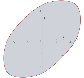
Figure 1. The Deninger chain $\Gamma$.

We obtain that $\partial\Gamma$ is contained completely in $C$, hence defines a cycle in $H_{1}(C(\mathbb{C}),\mathbb{Q}(2))^{+}$. By the following change of variables

$$x=-\dfrac{Y+X^{2}+1}{X(X-1)},\quad y=-\dfrac{Y}{X(X+X)}-\dfrac{1}{X},$$

we get the Jacobian of $C$ is given by

$$E/\mathbb{Q}:Y^{2}+XY+Y=X^{3}-X,$$

which is an elliptic curve of type $14a4$. Its torsion subgroup is $\mathbb{Z}/6\mathbb{Z}=\left<A\right>$ with $A=(-1,2)$. With the help of Magma [BCP], we have

$$\mathrm{div}(x)=-(5A)+(A)-(4A)+(2A),\quad\mathrm{div}(y)=(\mathcal{O})+(A)-(4A)-(3A).$$

Denote by $S$ the closed subscheme of $E$ consisting of all points in supports of above divisors. The values of $f_{j}$ and $f_{j}\circ\tau$ at $p\in S$ are either $0,1$ or $\infty$ for all $j$, then the elements $v_{p}(g_{j})\{f_{j}(p)\}_{2}$ and $v_{p}(g_{j}\circ\tau)\{f_{j}\circ\tau(p)\}_{2}$ are all trivial in $B_{2}(\mathbb{Q})$ for all $j$ and $p\in S$. Then by Theorem 0.1, we have the pure identity 5.1.2 condiationally on Beilinson's conjecture.

b) We study the pure identity (2) in Table 1

(5.1.3) $$\mathrm{m}(1+x+y+z+xy+xz+yz)\stackrel{{\scriptstyle?}}{{\sim}}_{\mathbb{Q}^{\times}}L^{\prime}(E_{14},-1).$$

First we notice that

$$\mathrm{m}(1+x+y+xy+z(1+x+y))=\mathrm{m}(1+x+y+z(1+x+y+xy)),$$

so it suffices to work on the following identity

(5.1.4) $$\mathrm{m}(1+x+y+z(1+x+y+xy))\stackrel{{\scriptstyle?}}{{\sim}}_{\mathbb{Q}^{\times}}L^{\prime}(E_{14},-1).$$

We have $\mathrm{m}(\tilde{P})=\mathrm{m}(1+x+y+xy)=\mathrm{m}(x+1)\mathrm{m}(y+1)=0$. We have the following decomposition

$$x\wedge y\wedge z =x\wedge(1+x)\wedge y\ -\ y\wedge(1+y)\wedge x\ +\ (x+y)\wedge(1+x+y)\wedge x$$

$$\quad-\ (x+y)\wedge(1+x+y)\wedge y\ -\ \dfrac{x}{y}\wedge(1+\dfrac{x}{y})\wedge(1+x+y),$$

so

$$f_{1}=-x,\quad f_{2}=-y,\quad f_{3}=f_{4}=-(x+y),\quad f_{5}=-x/y,\quad g_{1}=g_{4}=y,\quad g_{2}=g_{3}=x,\quad g_{5}=1+x+y.$$

The curve $W_{P}$ in this case is

$$x(x^{2}+1)y^{2}+(x^{2}+x+1)y+x+1=0,$$

and by using the following change of variable,

$$x=-\dfrac{Y+X^{2}+1}{X(X-1)},\quad y=\dfrac{Y}{X(X+1)},$$

its Jacobian is

$$E/\mathbb{Q}:Y^{2}+XY+Y=X^{3}-X,$$

which is the same elliptic curve as section (a). We have

$$\mathrm{div}(x)=-(5A)+(A)-(4A)+(2A),$$

$$\mathrm{div}(y)=(\mathcal{O})+(5A)-(2A)-(3A),$$

$$\mathrm{div}(1+x+y)=2(\mathcal{O})-(5A)+2(A)-(4A)-(2A)-(3A),$$

$$\mathrm{div}(1+1/a+1/b)=-(\mathcal{O})+2(4A)-(2A)+2(3A)-(5A)-(A).$$

With the same reason as the section (a), we get pure identity 5.1.4 conditionally on Beilinson's conjecture. Moreover, as mentioned in the introduction, we have

$$\mathrm{m}((1+x)(1+y)(x+y)+z)\stackrel{{\scriptstyle?}}{{\sim}}_{\mathbb{Q}^{\times}}\mathrm{m}(1+x+y+z+xy+xz+yz),$$

because they are rational multiples of the same elliptic curve $L$-value $L^{\prime}(E_{14},-1)$.

c) By the same method as in the previous section, we get the identity (11) in Table 1

$$\mathrm{m}(1+x+y+z+xy+xz+yz-xyz)\stackrel{{\scriptstyle?}}{{\sim}}_{\mathbb{Q}^{\times}}L^{\prime}(E_{36},-1).$$

This identity is interesting because this is the only case have been found with CM elliptic curve.

d) Similarly, we can prove most of pure identities in Table 1, excepted the identities (5),(6),(7) and (8). It suffices to consider identity (5) as Lalín and Nair showed that the polynomials in identities (5), (6), (7), and (8) share the same Mahler measure (see [LN]). We consider the identity (5):

(5.1.5) $$\mathrm{m}(1+(x+1)y+(x-1)z)\stackrel{{\scriptstyle?}}{{\sim}}_{\mathbb{Q}^{\times}}L^{\prime}(E_{21},-1),$$

where $P$ is of the form (5.1.1). We have the following decomposition

$$x\wedge y\wedge z=x\wedge(1-x)\wedge y+(x+1)y\wedge(1+(x+1)y)\wedge x-x\wedge(1+x)\wedge(1+(x+1)y),$$

so

$$f_{1}=-f_{3}=g_{2}=x,\quad f_{2}=-(x+1)y,\quad g_{1}=y,\quad g_{3}=1+(x+1)y,\quad f_{2}\circ\tau=-\dfrac{x+1}{xy},\quad g_{3}\circ\tau=\dfrac{xy+x+1}{xy}.$$

We have $W_{P}$ is given by $x(x+1)y^{2}+(2x^{2}+x+2)y+1+x=0,$ which is a non-singular curve of genus 1. Using the following change of variables

$$x=-\dfrac{X^{2}-6X+3Y}{X(X-6)},\quad y=\dfrac{Y-3X-3}{X(X+1)},$$

we get an equation for the Jacobian of $W_{P}$

$$E/\mathbb{Q}:Y^{2}-3XY-3Y=X^{3}-5X^{2}-6X$$

which is an elliptic curve of type $21a1$. Its torsion subgroup is $\mathbb{Z}/2\mathbb{Z}\times\mathbb{Z}/4\mathbb{Z}=\left<A\right>\times\left<B\right>$ with $A=(-1,0)$, and $B=(0,0)$. With the help of Magma [BCP], we have

$$\mathrm{div}(x)=-(A+B)+(A+3B)-(3B)+(B),$$

$$\mathrm{div}(y)=(\mathcal{O})+(A+B)-(B)-(A),$$

$$\mathrm{div}(1+(x+1)y)=2(2B)-(3B)-(B),$$

$$\mathrm{div}(xy+x+1)=(\mathcal{O})+2(A+2B)-(A+B)-(3B)-(A).$$

Let $S$ be the closed subscheme of $E$ consisting of all the points above. We have

$$\sum_{j}v_{B}(g_{j})\{f_{j}(B)\}_{2}+v_{B}(g_{j}\circ\tau)\{f_{j}\circ\tau(B)\}_{2} =v_{B}(g_{2})\{f_{2}(B)\}_{2}+v_{B}(g_{2}\circ\tau)\{f_{2}\circ\tau(B)\}_{2}$$

$$=\{\infty\}_{2}-\{1/2\}_{2}=\{2\}_{2},$$

which is nontrivial in $B_{2}(\mathbb{Q})$. As $S$ consists of points in $E_{\mathrm{tors}}$, we can choose $N$ in Theorem 0.1 equals to $\#E_{\mathrm{tors}}=8$. Since all the points of $S$ have rational coordinates, then the Bloch-Wigner dilogarithmic values in identity (0.0.8) all vanish. The Deninger chain and its boundary are described in polar coordinate $x=e^{it}$, $y=e^{it}$ for $s,t\in[-\pi,\pi]$ as follows

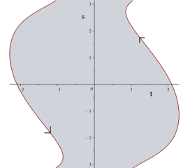
Figure 2. The Deninger chain $\Gamma$.

The boundary $\partial\Gamma$ consists of 2 loops and does not contain any zeros and poles of $f_{j},g_{j}$. Hence by Theorem 0.1, we get pure identities (5.1.5) conditionally on Beilinson's conjecture. In particular, under Beilinson's conjecture, we have

$$\mathrm{m}(1+(x+1)y+(x-1)z)\stackrel{{\scriptstyle?}}{{\sim}}_{\mathbb{Q}^{\times}}\mathrm{m}((x+1)^{2}(y+1)+z),$$

as they are rational multiples of $L^{\prime}(E_{21},-1)$.

e) There is an interesting remark on the identities (4) and (10) of Table 1. By some trivial change of variables, we obtain

$$\mathrm{m}((x+1)^{2}+(1-x)(y+z))=\mathrm{m}((x+1)(y+1)+(x-1)^{2}z).$$

We can apply theorem 0.1 to the the polynomial $P=(x+1)^{2}+(1-x)(y+z)$. However, it does not apply to $P=(x+1)(y+1)+(x-1)^{2}z$. Indeed, in this case, $W_{P}$ is given by

$$(-x^{3}-2x^{2}-x)y^{2}+(x^{4}-6x^{3}+2x^{2}-6x+1)y-x^{3}-2x^{2}-x=0,$$

which is an irreducible curve and has a singularity at $(1,-1)$. The figure below describes the Deninger chain $\Gamma$ (the shaded region) and the boundary $\partial\Gamma$ in polar coordinates $x=e^{it},y=e^{is}$ for $t,s\in[-\pi,\pi]$, which passes the singular point of $W_{P}$ (indicated by the marked points in the figure). Using Magma [BCP], we can check that it is no longer a loop on the normalization of $W_{P}$.

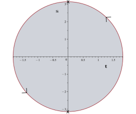
Figure 3. The Deinger chain $\Gamma$.

The same situation happens with the identity (10),

$$\mathrm{m}((1+x)^{2}+y+z)=\mathrm{m}(1+y+(1+x)^{2}z),$$

where we can apply Theorem 0.1 to the first polynomial but not to the second one.

f) Theorem 0.1 does not apply to the identity (1) in Table 2

$$\mathrm{m}(1+xy+(1+x+y)z)\stackrel{{\scriptstyle?}}{{\sim}}_{\mathbb{Q}^{\times}}L^{\prime}(E_{90},-1),$$

because there some $u_{p}$ are nontrivial and it violates the $N$-torsion condition in Theorem 0.1. First let us write the decomposition

$$x\wedge y\wedge z=xy\wedge(1+xy)\wedge x-(x+y)\wedge(1+x+y)\wedge x+(x+y)\wedge(1+x+y)\wedge y+\dfrac{-x}{y}\wedge\left(1+\dfrac{x}{y}\right)\wedge(1+x+y),$$

hence

$$f_{1}=-xy,\quad f_{2}=f_{3}=-(x+y),\quad f_{4}=-x/y,$$

$$g_{1}=g_{2}=x,\quad g_{3}=y,\quad g_{4}=1+x+y.$$

The curve $W_{P}$ is given by

$$(-x^{2}+x+1)y^{2}+(x^{2}+x+1)y+x^{2}+x-1=0,$$

which is an irreducible curve of genus 1 and does not contain any rational points. The figure below describes the Deninger chain and its boundary in polar coordinates. We find that $\partial\Gamma$ does not contain any singular points of $W_{P}$.

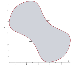
Figure 4. The Deninger chain $\Gamma$.

By Magma [BCP], we obtain that Jacobian of $C$ is given by

$$E/\mathbb{Q}:Y^{2}+XY+Y=X^{3}-X^{2}-8X+11,$$

which is an elliptic curve of type $90b1$. Its torsion subgroup is $\mathbb{Z}/6\mathbb{Z}=\left<A\right>$, with $A=(3,1)$. Denote by $K=\mathbb{Q}(\alpha)$ where $\alpha\in\mathbb{C}$ such that $\alpha^{2}+\alpha-1=0$. Let $B_{1}=(6\alpha+9,-24\alpha-35)$, $B_{2}=(-4\alpha+1,12\alpha-3)$, $B_{3}=(\frac{9}{5},\frac{24\alpha-23}{25})$, $B_{4}=(2,-\alpha-2)$, $B_{5}=(-6\alpha+3,-18\alpha+7)$, $B_{6}=(4\alpha+5,8\alpha+9)$ and we denote by $(B_{i})$ the divisor in $E$ corresponding to the point $B_{i}$. We have the following divisors in $E/K$

$$\mathrm{div}(x)=(4A)+(B_{1})-(A)-(B_{2}),$$

$$\mathrm{div}(y)=(\mathcal{O})+(B_{3})-(B_{4})-(3A),$$

$$\mathrm{div}(1+x+y)=2(2A)+2(B5)-(A)-(B_{4})-(3A)-(B_{2}),$$

$$\mathrm{div}(1+1/x+1/y)=-(\mathcal{O})+2(5A)+2(B_{6})-(B_{3})-(4A)-(B_{1}).$$

Denote by $S$ the closed subscheme of $E$ consisting of all these points. We have

$$\sum_{j}v_{B_{1}}(g_{j})\{f_{j}(B_{1})\}_{2}+v_{B_{1}}(g_{j}\circ\tau)\{f_{j}\circ\tau(B_{1})\}_{2} =v_{B_{1}}(g_{1})\{0\}_{2}+v_{B_{1}}(g_{1}\circ\tau)\{\infty\}_{2}$$

$$\quad+v_{B_{1}}(g_{2})\{-\alpha\}_{2}+v_{B_{1}}(g_{2}\circ\tau)\{\infty\}_{2}+v_{B_{1}}(g_{4}\circ\tau)\{\infty\}_{2}$$

$$=\{-\alpha\}_{2},$$

which is nontrivial in $B_{2}(K)$. The torsion condition in Theorem 0.1 does not satisfy since $B_{1}$ has infinite order in $E(K)$.

For the same reason as before, we fail to apply the main theorem to the identity (2) of Table 2

$$\mathrm{m}((1+x)(1+y)+(1-x-y)z)\stackrel{{\scriptstyle?}}{{\sim}}_{\mathbb{Q}^{\times}}L^{\prime}(E_{450},-1).$$

5.2. Identities with Dirichlet character

In this subsection, we investigate identities of the form

$$\mathrm{m}(P)\stackrel{{\scriptstyle?}}{{=}}a\cdot L^{\prime}(E,-1)+\sum_{\chi}b_{\chi}\cdot L^{\prime}(\chi,-1),$$

where $a\in\mathbb{Q},b_{\chi}\in\mathbb{Q}^{\times}$, $E$ is an elliptic curve and $\chi$ are odd quadratic Dirichlet characters.

a) We prove the identity (0.0.10) conditionally on Beilinson's conjecture. The polynomial $P$ is of the form (5.1.1), and we have the following decomposition on $V_{P}$

$$x\wedge y\wedge z =-\frac{1}{3}x^{3}\wedge(1-x^{3})\wedge y\ +\ x\wedge(1-x)\wedge y\ +\ (x^{2}-x+1)y\wedge(1+(x^{2}-x+1)y)\wedge x$$

$$\quad-\frac{1}{3}x^{3}\wedge(1+x^{3})\wedge(1+(x^{2}-x+1)y)\ +\ x\wedge(1+x)\wedge(1+(x^{2}-x+1)y).$$

We have

$$f_{1}=x^{3},\ f_{2}=x,\ f_{3}=-(x^{2}-x+1)y,\ f_{4}=-x^{3},f_{5}=-x,$$

$$g_{1}=g_{2}=y,\ g_{3}=x,\ g_{4}=g_{5}=1+(x^{2}-x+1)y.$$

The curve $W_{P}$ is defined by $x^{2}(x^{2}-x+1)y^{2}-x(4x^{2}-x+4)y+x^{2}-x+1=0,$ which is a non-singular curve of genus 1 and does not contain any non-singular rational point. By the change of variables $x=X,y=Y/X,$ we get a new equation

$$(X^{2}-X+1)Y^{2}-(4X^{2}-X+4)Y+X^{2}-X+1=0.$$

By Pari/GP [PARI], its Jacbian is given by the following Weierstrass form

$$E/\mathbb{Q}:v^{2}+uv=u^{3}-u^{2}-45u-104,$$

which is an elliptic of type $45a2$. We denote by $k=\mathbb{Q}(\alpha)$ with $\alpha^{2}-\alpha+1=0$. A base change of $E$ over $k$ can be given by

$$E_{k}:V^{2}+3UV+3V=U^{3}-U^{2}-9U,$$

by using the following change of variables

$$x =\dfrac{(2-\alpha)V+\alpha U^{2}-3(\alpha-1)U+3}{U^{2}+(4\alpha-2)U-3\alpha}$$

$$y =\dfrac{((1-\alpha)U^{2}-(\alpha+4)U+(\alpha+4))V+2\alpha U^{3}-(8\alpha-3)U^{2}+(3\alpha-12)U+12}{U^{4}-(4\alpha+1)U^{3}+(15\alpha-7)U^{2}-(17\alpha-13)U+6(\alpha-1)}.$$

The torsion subgroup of $E_{k}$ is $\mathbb{Z}/2\mathbb{Z}\times\mathbb{Z}/4\mathbb{Z}=\left<A\right>\times\left<B\right>$ with $A=(-3,3)$ and $B=(0,0)$. Let $K$ be the number field $\mathbb{Q}(\alpha,r,s)$ with

$$r^{2}-2(2\alpha-1)r+3(\alpha-1)=0,\text{ and }s^{2}+2(2\alpha-1)s-3\alpha=0.$$

We set $P_{1}=(r,\alpha r-2\alpha-2),\text{ and }P_{2}=(s,(1-\alpha)s+2\alpha-4)$ be points in $E(K)$ and denote by $(P_{i})$ the divisor corresponding to $P_{i}$ in $E_{k}$. We have the following divisors in $E_{k}$

$$\mathrm{div}(g_{3})=\mathrm{div}(x)=(P_{1})-(P_{2}),$$

$$\mathrm{div}(g_{1})=\mathrm{div}(g_{2})=\mathrm{div}(y)=(\mathcal{O})+(A+3B)-(A+B)+(P_{2})-(2B)-(P_{1}),$$

$$\mathrm{div}(g_{4})=\mathrm{div}(g_{5})=\mathrm{div}(1+(x^{2}-x+1)y)=2(3B)+2(A)-(P_{1})-(P_{2}),$$

$$\mathrm{div}(g_{4}\circ\tau)=\mathrm{div}(g_{5}\circ\tau)=\mathrm{div}(1+(1/x^{2}-1/x+1)(1/y))=2(B)+2(A+2B)-(P_{1})-(P_{2}).$$

The values of $f_{j}$ and $f_{j}\circ\tau$ at $P_{1},P_{2}$ and their conjugates are either 0 or $\infty$, so we only concern about the other points. We obtain that

$$u_{A} =v_{A}(g_{4})\{f_{4}(A)\}_{2}+v_{A}(g_{5})\{f_{5}(A)\}_{2}=\{-1\}_{2}+\{1/\alpha\}_{2}=-\{\alpha\}_{2},$$

$$u_{B} =v_{B}(g_{4}\circ\tau)\{f_{4}\circ\tau(B)\}_{2}+v_{B}(g_{5}\circ\tau)\{f_{5}\circ\tau(B)\}_{2}$$

$$=2\{-1\}_{2}+2\{\alpha\}_{2}=2\{\alpha\}_{2},$$

$$u_{2B} =v_{2B}(g_{1})\{f_{1}(2B)\}_{2}+v_{2B}(g_{1}\circ\tau)\{f_{1}\circ\tau(2B)\}_{2}+v_{2B}(g_{2})\{f_{2}(2B)\}_{2}+v_{2B}(g_{2}\circ\tau)\{f_{2}\circ\tau(2B)\}_{2}$$

$$=-\{-1\}_{2}+\{-1\}_{2}-\{1/\alpha\}_{2}+\{\alpha\}_{2}=2\{\alpha\}_{2},$$

$$u_{3B} =v_{3B}(g_{4})\{f_{4}(3B)\}_{2}+v_{3B}(g_{5})\{f_{5}(3B)\}_{2}=2\{-1\}_{2}+2\{\alpha\}_{2}=2\{\alpha\}_{2},$$

$$u_{A+B} =v_{A+B}(g_{1})\{f_{1}(A+B)\}_{2}+v_{A+B}(g_{1}\circ\tau)\{f_{1}\circ\tau(A+B)\}_{2}$$

$$\quad+v_{A+B}(g_{2})\{f_{2}(A+B)\}_{2}+v_{A+B}(g_{2}\circ\tau)\{f_{2}\circ\tau(A+B)\}_{2}$$

$$=-\{-1\}_{2}+\{-1\}_{2}-\{\alpha\}_{2}+\{1/\alpha\}_{2}=-2\{\alpha\}_{2},$$

$$u_{A+2B} =v_{A+2B}(g_{4}\circ\tau)\{f_{4}\circ\tau(A+2B)\}_{2}=2\{-1\}_{2}+2\{1/\alpha\}_{2}=-2\{\alpha\}_{2}$$

$$u_{A+3B} =v_{A+3B}(g_{1})\{f_{1}(A+3B)\}_{2}+v_{A+3B}(g_{1}\circ\tau)\{f_{1}\circ\tau(A+3B)\}_{2}$$

$$\quad+v_{A+3B}(g_{2})\{f_{2}(A+3B)\}_{2}+v_{A+3B}(g_{2}\circ\tau)\{f_{2}\circ\tau(A+3B)\}_{2}$$

$$=\{-1\}_{2}-\{-1\}_{2}+\{1/\alpha\}_{2}-\{\alpha\}_{2}=-2\{\alpha\}_{2},$$

which are nontrivial in $B_{2}(K)$. Notice that $P_{1},P_{2}$ have order 8 in $E(K)$ and all the other points belong to the torsion subgroup of $E_{k}$, hence we choose $N$ in Theorem 0.1 equals to 8. The following figure indicates the Deninger chain (the shaded region) and its (oriented) boundary in polar coordinates $x=e^{it},y=e^{is}$ for $s,t\in[-\pi,\pi]$.

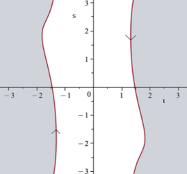
Figure 5. The Deninger chain $\Gamma$.

The boundary $\partial\Gamma$ consists of 2 loops, and does not contain any zeros and poles of $f_{j},g_{j}$. Moreover, by the equation (4.2.3), we have $\mathrm{m}(P)=-\dfrac{1}{8\pi^{2}}\int_{\partial\Gamma}\rho(\lambda),$ so $\partial\Gamma$ must be nontrivial as otherwise $m(P)$ vanishes. Hence $\partial\Gamma$ defines a generator of $H_{1}(C(\mathbb{C}),\mathbb{Z})^{+}$. Then by Theorem 0.1, we get

$$\mathrm{m}(1+(x^{2}-x+1)y+(x^{2}+x+1)z)\stackrel{{\scriptstyle?}}{{=}}a\cdot L^{\prime}(E_{45},-1)+\dfrac{b}{32\pi}\cdot D(\alpha),\ a\in\mathbb{Q}^{\times},b\in\mathbb{Z}\setminus\{0\},$$

under Belinson's conjecture. We are unable to determine the coefficient $b$ as computing the integrals $\int_{\partial\Gamma}\ d\arg f_{p}$ for $p\in S$ is difficult. By Remark 4.22, we have

$$D(\alpha)=\dfrac{3\sqrt{3}}{4}L(\chi_{-3},2)=\pi L^{\prime}(\chi_{-3},-1).$$

Finally, we get

$$\mathrm{m}(1+(x^{2}-x+1)y+(x^{2}+x+1)z)\stackrel{{\scriptstyle?}}{{=}}a\cdot L^{\prime}(E_{45},-1)+\dfrac{b}{32}\cdot L^{\prime}(\chi_{-3},-1),\ a\in\mathbb{Q}^{\times},b\in\mathbb{Z}\setminus\{0\}.$$

b) Using a method of Lalín [Lal15, § 4.2], we prove unconditionally the following identity involving only the $L$-value of Dirichlet character $\chi_{-4}$

$$\mathrm{m}(x^{2}+1+(x+1)^{2}y+(x-1)^{2}z)=2L^{\prime}(\chi_{-4},-1).$$

which is the identity (6) of Table 4. We have $\mathrm{m}(\tilde{P})=0$. We have the following decomposition on $V_{P}$

$$x\wedge y\wedge z =-\dfrac{1}{2}x^{2}\wedge(1+x^{2})\wedge y+2x\wedge(1-x)\wedge y+x\wedge\dfrac{(x+1)^{2}y}{x^{2}+1}\wedge\left(1+\dfrac{(x+1)^{2}y}{x^{2}+1}\right)$$

$$\quad-2x\wedge(1+x)\wedge\left(1+\dfrac{(x+1)^{2}y}{x^{2}+1}\right)+\dfrac{1}{2}x^{2}\wedge(1+x^{2})\wedge\left(1+\dfrac{(x+1)^{2}y}{x^{2}+1}\right).$$

We have

$$\rho(\xi) =-\dfrac{1}{2}\rho(-x^{2},y)+2\rho(x,y)+\rho\left(\dfrac{-(x+1)^{2}y}{x^{2}+1},x\right)-2\rho\left(-x,1+\dfrac{(x+1)^{2}y}{x^{2}+1}\right)+\dfrac{1}{2}\rho\left(-x^{2},1+\dfrac{(x+1)^{2}y}{x^{2}+1}\right),$$

where

$$\rho(f,g)=-D(f)d\arg g+\dfrac{1}{3}\log|g|(\log|1-f|d\log|f|-\log|f|d\log|1-f|).$$

We have $W_{P}$ is given by

$$(x^{2}+1)((x+1)^{2}y^{2}+(x^{2}+8x+1)y+(x+1)^{2})=0,$$

which is the union of $L:x^{2}+1=0$ and the curve $C:(x+1)^{2}y^{2}+(x^{2}+8x+1)y+(x+1)^{2}=0$. The figure below describes the Deninger chain $\Gamma$ in polar coordinates

$$\Gamma:\left|\dfrac{x^{2}+1+(x+1)^{2}y}{(x-1)^{2}}\right|\geq 1,x=e^{it},y=e^{is},s,t\in[-\pi,\pi].$$

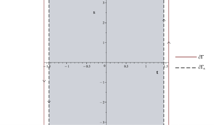
Figure 6. The integration domain.

Its boundary $\partial\Gamma$ consists of 2 loops $\gamma=\{t=\pi/2,-\pi\leq s\leq\pi\}\text{ and }\delta=\{t=-\pi/2,-\pi\leq s\leq\pi\}$ (with orientations as shown in the figure), which are contained in $L$. As $\partial\Gamma$ contains poles of $\rho(\xi)$, we do not have (4.2.5) directly. We adjust the Deninger chain as follows, for $\varepsilon>0$

$$\Gamma_{\varepsilon}:\left|\dfrac{x^{2}+1+(x+1)^{2}y}{(x-1)^{2}}\right|\geq 1,x=e^{i(1+\varepsilon)t},y=e^{is},\text{ for }s,t\in[-\pi,\pi],$$

which is the shaded region in Figure 6 with the boundary $\partial\Gamma_{\varepsilon}=\gamma_{\varepsilon}\cup\delta_{\varepsilon}$, where

$$\gamma_{\varepsilon}=\{t=\dfrac{\pi}{2(1+\varepsilon)},-\pi\leq s\leq\pi\},\quad\delta_{\varepsilon}=\{t=-\dfrac{\pi}{2(1+\varepsilon)},-\pi\leq s\leq\pi\}.$$

Recall differential forms $\eta$ and $\rho(\lambda)$ defined in equation (4.1.1) and Definition 4.4 respectively. We have

(5.2.1) $$\int_{\Gamma_{\varepsilon}}\eta=\int_{\partial\Gamma_{\varepsilon}}\rho(\xi)=\dfrac{1}{2}\int_{\partial\Gamma_{\varepsilon}}\rho(\lambda),$$

where the first equality is obtained by using Stokes's theorem and the second equality can be proven as in the proof of Lemma 4.10. As $\rho(\lambda)$ is a closed differential form, we can take the limit of equation (5.2.1) as $\varepsilon\to 0$ without changing the value of the integration, and so that

$$\mathrm{m}(P)=-\dfrac{1}{4\pi^{2}}\lim_{\varepsilon\to 0}\int_{\partial\Gamma_{\varepsilon}}\rho(\xi).$$

We have

$$\int_{\partial\Gamma_{\varepsilon}}\rho(\xi) =\int_{\partial\Gamma_{\varepsilon}}-\dfrac{1}{2}\rho(-x^{2},y)+2\rho(x,y)+\rho\left(\dfrac{-(x+1)^{2}y}{x^{2}+1},x\right)$$

$$\hskip 56.9055pt-2\rho\left(-x,1+\dfrac{(x+1)^{2}y}{x^{2}+1}\right)+\dfrac{1}{2}\rho\left(-x^{2},1+\dfrac{(x+1)^{2}y}{x^{2}+1}\right)$$

$$=\int_{\gamma_{\varepsilon}\cup\delta_{\varepsilon}}2\rho(x,y)-2\rho\left(-x,1+\dfrac{(x+1)^{2}y}{x^{2}+1}\right)$$

$$=\int_{\gamma_{\varepsilon}\cup\delta_{\varepsilon}}-2D(x)d\arg(y)+2D(-x)d\arg\left(1+\dfrac{(x+1)^{2}y}{x^{2}+1}\right)$$

$$=\left(-2D(e^{\frac{i\pi}{2(1+\varepsilon)}})\int_{\gamma_{\varepsilon}}d\arg(y)-2D(e^{-\frac{i\pi}{2(1+\varepsilon)}})\int_{\delta_{\varepsilon}}d\arg(y)\right)$$

$$\quad+\left(2D(-e^{\frac{i\pi}{2(1+\varepsilon)}})\int_{\gamma_{\varepsilon}}d\arg\left(1+\dfrac{(x+1)^{2}y}{x^{2}+1}\right)\right)+2D(-e^{-\frac{i\pi}{2(1+\varepsilon)}})\int_{\delta_{\varepsilon}}d\arg\left(1+\dfrac{(x+1)^{2}y}{x^{2}+1}\right).$$

We have

$$\int_{\gamma_{\varepsilon}}d\arg(y)=\int_{-\pi}^{\pi}ds=2\pi,\quad\int_{\delta_{\varepsilon}}d\arg y=\int_{\pi}^{-\pi}ds=-2\pi.$$

And

$$\int_{\gamma_{\varepsilon}}d\arg\left(1+\dfrac{(x+1)^{2}y}{x^{2}+1}\right)=2\pi,\quad\int_{\delta_{\varepsilon}}d\arg\left(1+\dfrac{(x+1)^{2}y}{x^{2}+1}\right)=-2\pi,$$

by looking at the figure below and the fact that $\left|\frac{(x+1)^{2}}{x^{2}+1}\right|>1$.

Figure 7. The argument of $1+ay$ with $|a|>1$.

Then we have $\lim_{\varepsilon\to 0}\int_{\partial\Gamma_{\varepsilon}}\rho(\xi)=-16\pi D(e^{i\pi/2})$. Hence

$$\mathrm{m}(P)=\dfrac{4}{\pi}D(e^{i\pi/2})=2L^{\prime}(\chi_{-4},-1).$$

We can do same with identities (4), (5), (7), (8) of Table 4.

c) Let study the identity (1) of Table 4, which involves only the $L$-value of Dirichlet character $\chi_{-3}$

$$\mathrm{m}(1+(x+1)(x^{2}+x+1)y+(x+1)^{3}z)=3L^{\prime}(\chi_{-3},-1).$$

We have $W_{P}$ is given by $(x^{2}+x+1)((x^{4}+x^{3})y^{2}+(-2x^{3}-5x^{2}-2x)y+x+1)=0$, which consists of the line $L:x^{2}+x+1=0$ and the curve $C:(x^{4}+x^{3})y^{2}+(-2x^{3}-5x^{2}-2x)y+x+1=0$. The figure below describes the integration domain in local coordinates $x=e^{it}$ and $y=e^{is}$ for $s,t\in[-\pi,\pi]$. The shaded region indicates the adjusted Denginger chain $\Gamma_{\varepsilon}$.

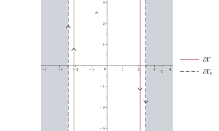
Figure 8. The integration domain.

We obtain that $\partial\Gamma=\gamma\cup\delta$ with

$$\gamma=\{t=2\pi/3,-\pi\leq s\leq\pi\}\text{ and }\delta=\{t=-2\pi/3,-\pi\leq s\leq\pi\},$$

which are contained in $L$. The differential $\rho(\xi)$ is not well-defined on $\partial\Gamma$. By the same computation as in the example (b), we have

$$\mathrm{m}(P)=-\dfrac{1}{4\pi^{2}}\lim_{\varepsilon\to 0}\int_{\partial\Gamma_{\varepsilon}}\rho(\xi)=3L^{\prime}(\chi_{-3},-1).$$

And this situation also happens with the identities (2) and (3) of Table 4.

d) Theorem 0.1 does not apply to identity (1) in Table 3

$$\mathrm{m}(x^{2}+x+1+(x^{2}+x+1)y+(x-1)^{2})\stackrel{{\scriptstyle?}}{{=}}-\dfrac{1}{12}L^{\prime}(E_{72},-1)+\dfrac{3}{2}L^{\prime}(\chi_{3},-1),$$

because of the same reason as the example 5.1(e). Indeed, the curve $W_{P}$ is given by

$$(x^{2}+x+1)^{2}y^{2}+(x^{4}+8x^{3}+8x+1)y+(x^{2}+x+1)^{2}=0,$$

which is irreducible and singular at $(1,-1)$. And $\partial\Gamma$ passes this singular point (indicated by the marked points in the following figure).

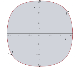
Figure 9. The Deninger chain $\Gamma$.

Using [BCP], we see that $\partial\Gamma$ is no longer a loop in the normalization of $W_{P}$.

e) We study the identity (2) of Table 3

$$\mathrm{m}(x^{2}+1+(x+1)^{2}y+(x^{2}-1)z)\stackrel{{\scriptstyle?}}{{=}}-\dfrac{1}{10}L^{\prime}(E_{48},-1)+L^{\prime}(\chi_{-4},-1),$$

We will show that this identity does not satisfy some conditions in Theorem 0.1, but we can still give some evidence to expect that this conjecture identity holds. We have

$$x\wedge y\wedge z =-\dfrac{1}{2}x^{2}\wedge(1+x^{2})\wedge y\ +\ \dfrac{1}{2}x^{2}\wedge(1-x^{2})\wedge y\ +\ \dfrac{(x+1)^{2}y}{x^{2}+1}\wedge\left(1+\dfrac{(x+1)^{2}y}{x^{2}+1}\right)\wedge x$$

$$\quad-2x\wedge(1+x)\wedge\left(1+\dfrac{(x+1)^{2}y}{x^{2}+1}\right)\ +\ \dfrac{1}{2}x^{2}\wedge(1+x^{2})\wedge\left(1+\dfrac{(x+1)^{2}y}{x^{2}+1}\right).$$

Then

$$\rho(\xi)=-\dfrac{1}{2}\rho(-x^{2},y)+\dfrac{1}{2}\rho(x^{2},y)+\rho\left(-\dfrac{(x+1)^{2}y}{x^{2}+1},x\right)-2\rho\left(-x,1+\dfrac{(x+1)^{2}y}{x^{2}+1}\right)+\dfrac{1}{2}\rho\left(-x^{2},1+\dfrac{(x+1)^{2}y}{x^{2}+1}\right).$$

The $W_{P}$ is given by

$$(x^{2}+1)((x+1)^{2}y^{2}+(3x^{2}+4x+3)y+(x+1)^{2})=0,$$

which is the union of $L:x^{2}+1=0$ and the curve $C:(x+1)^{2}y^{2}+(3x^{2}+4x+3)y+(x+1)^{2}=0,$ which is a nonsingular curve of genus 1. The following figure describes the Deninger chain $\Gamma$ and its boundary $\partial\Gamma$ in polar coordinate $x=e^{it}$ and $y=e^{is}$ for $t,s\in[-\pi,\pi]$.

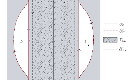
Figure 10. The Deninger chain $\Gamma$.

We have $\Gamma=\Gamma_{1}\cup\Gamma_{2}$, where $\Gamma_{1}$ is the shaded region in the center with the boundary

$$\partial\Gamma_{1}=\{t=-\pi/2,-\pi\leq s\leq\pi\}\cup\{t=\pi/2,-\pi\leq s\leq\pi\},$$

and $\Gamma_{2}$ is the shaded region with the boundary $\partial\Gamma_{2}$ as in the figure. We observe that $\partial\Gamma_{1}$ is contained in $L$ and $\partial\Gamma_{2}$ is contained in $C$. We have

$$\mathrm{m}(P)=m_{1}+m_{2},$$

where $m_{1}$ can be computed by the same method as the example (b):

$$m_{1}=-\dfrac{1}{4\pi^{2}}\int_{\Gamma_{1}}\eta=-\dfrac{1}{4\pi^{2}}\lim_{\varepsilon\to 0}\int_{\Gamma_{1,\varepsilon}}\eta=-\dfrac{1}{4\pi^{2}}\lim_{\varepsilon\to 0}\int_{\partial\Gamma_{1,\varepsilon}}\rho(\xi)=L^{\prime}(\chi_{-4},-1),$$

and

$$m_{2}=-\dfrac{1}{4\pi^{2}}\int_{\Gamma_{2}}\eta=-\dfrac{1}{4\pi^{2}}\int_{\partial\Gamma_{2}}\rho(\xi).$$

Let us explain how Theorem 0.1 does not apply to compute $m_{2}$. By the following change of variables

$$x=-\dfrac{2Y+X^{2}}{X^{2}-2X-4},\quad y=-\dfrac{2}{X+2},$$

the Jacobian of $C$ is given by

$$E/\mathbb{Q}:Y^{2}=X^{3}+X^{2}-4X-4,$$

which an elliptic curve of type $48a1$. Its torsion subgroup is $\mathbb{Z}/2\mathbb{Z}\times\mathbb{Z}/2\mathbb{Z}=\left<A\right>\times\left<B\right>$ where $A=(2,0)$ and $B=(-1,0)$. Set $K=\mathbb{Q}(\alpha,\beta)$ where $\alpha^{2}-2\alpha-4=0$ and $\beta^{2}+4=0$. Write

$$P_{1}=(\alpha,\alpha+2),P_{2}=(\alpha,-\alpha-2),P_{3}=(0,s,1).$$

We have

$$\mathrm{div}(x)=-(P_{1})+(P_{2}), \mathrm{div}\left(\frac{1+(1+x)^{2}y}{x^{2}+1}\right) =2(A)+2(A+B)-2(P_{3}),$$

$$\mathrm{div}(y)=2(\mathcal{O})-2(A+B), \mathrm{div}\left(\frac{x^{2}y+x^{2}+2x+y+1}{y(x^{2}+1)}\right) =2(\mathcal{O})+2(B)-2(R).$$

We have $u_{A}=u_{B}=u_{A+B}=0$ and $u_{P_{3}}=-2\{-\beta/2\}_{2}-2\{\beta/2\}_{2}=-2\{i\}_{2}+2\{i\}_{2}=0.$ And

$$u_{P_{1}} =-\{(-\alpha+4)/2\}_{2}+\{(\alpha+2)/2\}_{2}=2\{(\alpha+2)/2\}_{2},$$

$$\quad u_{P_{2}} =\{(-\alpha+4)/2\}_{2}-\{(\alpha+2)/2\}_{2}=-2\{(\alpha+2)/2\}_{2},$$

which are nontrivial in Bloch group. Using Magma, we obtain that $P_{1},P_{2}$ have infinite order in $E(K)$. Thus it violates the $N$-torsion condition in Theorem 0.1. Finally, we have

$$\mathrm{m}(P)=L^{\prime}(\chi_{-4},-1)+m_{2}.$$

References

- [Bloch] S. Bloch, Lectures on algebraic cycles, Cambridge University Press, second edition, 2010.
- [BCP] W. Bosma, J. Cannon, C. Playoust, The Magma algebra system I. The user language, J. Symbolic Comput., 24 (1997), 235–265.
- [Boy98] D. W. Boyd, Mahler’s measure and special values of -functions, Experiment. Math. 7 (1998), 37–82.
- [Boy06] D. W. Boyd, Conjectural explicit formulas for the Mahler measure of some three variable polynomials, unpublished notes, 2006.
- [Bur94] J. I. Burgos, A logarithmic Dolbeault complex, Compositio Math. 92 (1994), no. 1, 61–86.
- [Bur97] J. I. Burgos, Arithmetic Chow rings and Deligne–Beilinson cohomology, J. Algebraic Geom. 6 (1997), no. 2, 335–377.
- [Bru16] F. Brunault, Regulators of Siegel units and applications, Journal of Number Theory, Volume 163, 2016, Pages 542-569, ISSN 0022-314X.
- [Bru20] F. Brunault, Unpublished list of conjectural identities for 3-variable Mahler measures, 2020.
- [Bru22] F. Brunault, On the group of modular curves, arXiv:2009.07614.
- [Bru23] F. Brunault, On the Mahler measure of , arXiv:2305.02992.
- [BZ] F. Brunault, W. Zudilin, Many Variations of Mahler Measures, A Lasting Symphony, Cambridge University Press, 2020.
- [dJ95] R. De Jeu, Zagier’s conjecture and wedge complexes in algebraic -theory, Compositio Math. 96 (1995), no. 2, 197–247.
- [dJ96] R. De Jeu, On of curves over number fields, Invent. Math. 125 (1996), no. 3, 523–556.
- [dJ00] R. De Jeu, Towards regulator formulae for the -theory of curves over number fields, Compositio Math. 124 (2000), no. 2, 137–194.
- [Den97] C. Deninger, Deligne periods of mixed motives, K-theory and the entropy of certain -actions, J. Amer. Math. Soc. 10 (1997), no. 2, 259–281.
- [DS] C. Deninger, A. J. Scholl, The Beilinson conjecture, Cambridge University Press, 1991, 173-210.
- [FG] Eric M. Friedlander, Daniel R. Grayson, Handbook of -theory, Springer-Verlag Berlin Heidelberg 2005.
- [Gon95] A. B. Goncharov, Geometry of configuration, polylogarithms and motivic cohomomogy, Adv. in Math 114, (1995). 197-318.
- [Gon96] A. B. Goncharov, Deninger’s conjecture on L-functions of elliptic curves at , J. Math. Sci. (N. Y.) 81 (1996), no. 3, 2631–2656.
- [Gon98] A. B. Goncharov, Explicit regulator maps on polylogarithmic motivic complexes, Motives, polylogarithms and Hodge theory, Part I (Irvine, CA, 1998), 245–276, Int. Press Lect. Ser., 3, I, Int. Press, Somerville, MA, 2002. math.AG/0003086.
- [Kah] B. Kahn, Zeta and -Functions of Varieties and Motives, Cambridge University Press 462, 2020.
- [Lal10] M. N. Lalín, On a conjecture by Boyd, Int. J. Number Theory 6 (2010), no. 3, 705–711.
- [Lal15] M. N. Lalín, Mahler measure and elliptic curve -function at , J. Reine Angew. Math. 709 (2015), 201-218.
- [LR] M. N. Lalín and M. D. Rogers, Functional equations for Mahler measures of genus-one curves, Algebra Number Theory 1 (2007), no. 1, 87–117.
- [LN] M. N. Lalín and S. S. Nair, An invariant property of Mahler measure, Bull. Lond. Math. Soc. 55, (2023), no. 3, 1129–1142
- [LSZ] M. Lalín, D. Samart and W. Zudilin, Further explorations of Boyd's conjectures and a conductor 21 elliptic curve, J. Lond. Math. Soc., 93(2):341–360, 2016.
- [Mah] K. Mahler, On some iqualities for polynomials in several variables, Journal London Math. Soc. 37, 1962, 341-344.
- [Mai] V. Maillot, Mahler measure in Arakelov geometry, workshop lecture at "The many aspects of Mahler's measure", Banff International Research Station, Banff 2003.
- [MNP] Jacob P. Murre, Jan Nagel, Chris A. M. Peters, Lectures on the Theory of Pure Motives, AMS, University Lecture Series 61.
- [Nek] J. Nekovár̆, Beilinson's conjectures, in Motives (Seattle, WA, 1991), Proc. Sympos. Pure Math. 55 (Amer. Math. Soc., Providence, RI, 2013).
- [PARI] The PARI Group, PARI/GP version 2.16.0, Univ. Bordeaux, 2022, http://pari.math.u-bordeaux.fr/.
- [Rod] F. Rodriguez-Villegas, Modular Mahler measures I, in: Topics in number theory, (University Park 1997), Math. 467, Kluwer Academic, Dordrecht (1999), 17–48.
- [RZ] M. Rogers and W. Zudilin, On the Mahler measure of , Int. Math. Res. Not. IMRN, 9, 2305-2326, 2014.
- [Sul] A. Sulin, group of a field and the Bloch group, In Proceedings of the Steklov Math. Institute, 1991.
- [VSF] V. Voevodsky, A. Suslin, M. Friedlander, Cycles, Transfers and Motivic homology theories, Annals of Mathematics Studies 143, Princeton University Press, Princeton 2000.
- [Wei] C. Weibel, The -book: An introduction to algebraic -theory, Graduate Studies in Math. 145, AMS, 2013.
- [Zag] D. Zagier, Polylogarithms, Dedekind Zeta functions, and the Algebraic -theory of Fields, Arithmetic algebraic geometry (Texel, 1989), 391–430, Progr. Math., 89, Birkhuser Boston, Boston, MA, 1991.