Training-free linear image inversion via flows

Abstract

Training-free linear inversion involves the use of a pretrained generative model and—through appropriate modifications to the generation process—solving inverse problems without any finetuning of the generative model. While recent prior methods have explored the use of diffusion models, they still require the manual tuning of many hyperparameters for different inverse problems. In this work, we propose a training-free method for image inversion using pretrained flow models, leveraging the simplicity and efficiency of Flow Matching models, using theoretically-justified weighting schemes and thereby significantly reducing the amount of manual tuning. In particular, we draw inspiration from two main sources: adopting prior gradient correction methods to the flow regime, and a solver scheme based on conditional Optimal Transport paths. As pretrained diffusion models are widely accessible, we also show how to practically adapt diffusion models for our method. Empirically, our approach requires no problem-specific tuning across an extensive suite of noisy linear image inversion problems on high-dimensional datasets, ImageNet-64/128 and AFHQ-256, and we observe that our flow-based method for image inversion significantly improves upon closely-related diffusion-based linear inversion methods.

1 Introduction

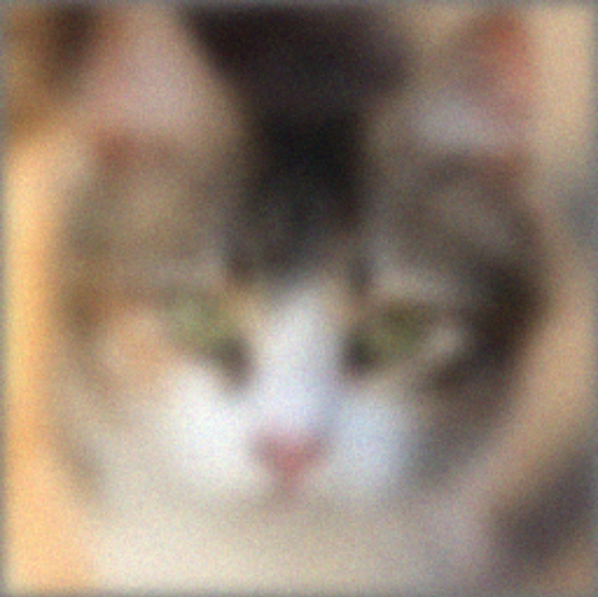
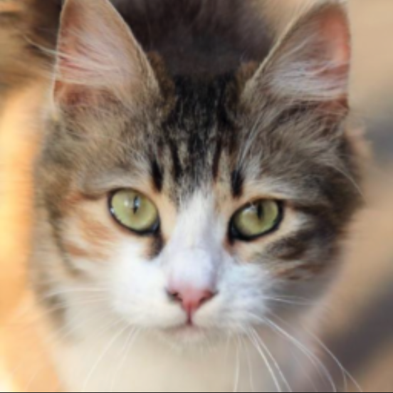
(a) Gaussian deblur

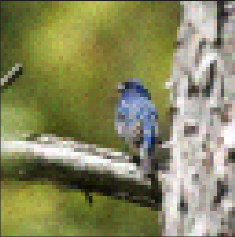
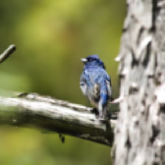
(b) $2\times$ Super-resolution

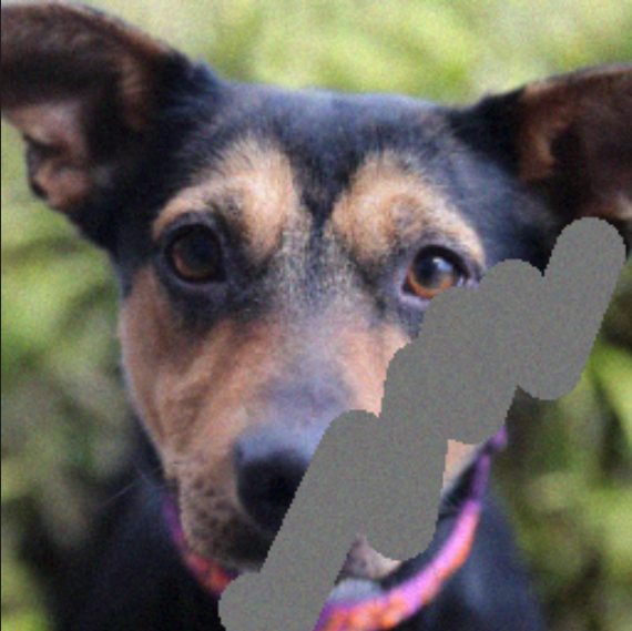
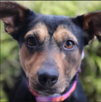
(c) Inpainting

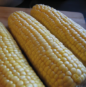
(d) Inpainting

Figure 1: Corrected images by solving linear inverse problems with flow models. For each pair of images, we show the noisy measurement (left) and the reconstruction (right).

The problem of image inversion involves recovering a clean image from noisy measurements generated by a known degradation model. Many interesting image processing tasks can be cast as image inversion. Some instances of these problems are super-resolution, inpainting, deblurring, colorization, denoising etc. Diffusion models or score-based generative models (Sohl-Dickstein et al., 2015; Ho et al., 2020; Song & Ermon, 2019; Song et al., 2021c) have emerged as a leading family of generative models for solving image inversion problems (Saharia et al., 2022b; a; Wang et al., 2022; Chung et al., 2022a; Song et al., 2022; Mardani et al., 2023). However, sampling with diffusion models is known to be slow, and the quality of generated images is affected by the curvature of SDE/ODE solution trajectories (Karras et al., 2022). While Karras et al. (2022) observed ODE sampling for image generation could produce better results, sampling via SDE is still common for image inversion, whereas ODE sampling has been rarely considered, perhaps due to the use of diffusion probability paths.

Continuous Normalizing Flow (CNF) (Chen et al., 2018) trained with Flow Matching (Lipman et al., 2022) has been recently proposed as a powerful alternative to diffusion models. CNF (hereafter denoted flow model) has the ability to model arbitrary probability paths, and includes diffusion probability paths as a special case. Of particular interest to us are Gaussian probability paths that correspond to optimal transport (OT) displacement (McCann, 1997). Recent works (Lipman et al., 2022; Albergo & Vanden-Eijnden, 2022; Liu et al., 2022; Shaul et al., 2023) have shown that these conditional OT probability paths are straighter than diffusion paths, which results in faster training and sampling with these models. Due to these properties, conditional OT flow models are an appealing alternative to diffusion models for solving image inversion problems.

In this work, we introduce a training-free method to utilize pretrained flow models for image inversion tasks. Our approach adds a correction term to the vector field that takes into account knowledge from the degradation model. Specifically, we introduce an algorithm that incorporates $\Pi$GDM (Song et al., 2022) gradient correction to flow models. Given the wide availability of pretrained diffusion models, we also present a way to convert these models to arbitrary paths for our sampling procedure. Empirically, we observe images restored via a conditional OT path consistently exhibit perceptual quality better than that achieved by the model’s original diffusion path as well as recently proposed diffusion approaches, such as $\Pi$GDM (Song et al., 2022) and RED-Diff (Mardani et al., 2023), across all linear image inversion tasks. To summarize, our key contributions are:

• We present a training-free algorithm for image inversion with pretrained conditional OT flow models that adapts the $\Pi$GDM correction, proposed for diffusion models, to flow sampling.

• We offer a way to convert between flow models and diffusion models, enabling the use of pretrained continuous-time diffusion models for conditional OT sampling, and vice versa.

• We demonstrate images restored via our algorithm using conditional OT probability paths have perceptual quality that is on par with, or better than that achieved by diffusion probability paths, and other recent methods like $\Pi$GDM and RED-Diff.

2 Preliminaries

We introduce relevant background knowledge and notation from conditional diffusion and flow modeling, as well as training-free inference with diffusion models.

Notation.

Both diffusion and flow models consider two distinct processes indexed by time between $[0,1]$ that convert data to noise and noise to data. Here, we follow the temporal notation used in prior work (Lipman et al., 2022) where the distribution at $t=1$ is the data distribution and $t=0$ is a standard Gaussian distribution. Note that this is opposite of the prevalent notation used in diffusion model literature (Song & Ermon, 2019; Ho et al., 2020; Song et al., 2021a; c). We let ${\bm{x}}_{t}$ denote the value at time $t$, without regard to which process (i.e., diffusion or flow) it was drawn from. The probability density for the data to noise process is denoted $q$ and the parameterized probability density for the noise to data process is denoted $p_{\theta}$. Expectations with respect to $q$ are denoted via $\mathbb{E}_{q}$. We generally keep function arguments of $t$ implicit (i.e. $f({\bm{x}}_{t},t)$ is informally written as $f({\bm{x}}_{t})$.)

Conditional diffusion models.

Conditional diffusion uses a limited class of processes $q$, and defines data to noise process $p_{\theta}$ as a Markov process that in continuous time obeys a stochastic differential equation (SDE) (Song & Ermon, 2019; Ho et al., 2020; Song et al., 2021c). The parameters of $p_{\theta}$ are learned via minimizing a regression loss with respect to $\widehat{{\bm{x}}_{1}}$

$$L_{\text{diffusion}}(\widehat{{\bm{x}}_{1}},q)=\int_{0}^{1}w(t)\mathbb{E}_{q}[(\widehat{{\bm{x}}_{1}}({\bm{x}}_{t},{\bm{y}})-{\bm{x}}_{1})^{2}]dt$$ (1)

where $w(t)$ are positive weights (Kingma et al., 2021; Song et al., 2021b; Kingma & Gao, 2023), ${\bm{y}}$ is conditioning (i.e. a noisy image), and ${\bm{x}}_{1}$ is noiseless data. The optimal solution for $\widehat{{\bm{x}}_{1}}$ is $\mathbb{E}_{q}[{\bm{x}}_{1}|{\bm{x}}_{t},{\bm{y}}]$, and hence we refer to $\widehat{{\bm{x}}_{1}}$ as a denoiser. Many equivalent parameterizations exist and have known conversions to denoising. Sampling using $p_{\theta}$ proceeds via starting from ${\bm{x}}_{0}\sim p_{\theta}({\bm{x}}_{0}|{\bm{y}})$ and integrating the SDE to $t=1$. If $p_{\theta}({\bm{x}}_{0}|{\bm{y}})=q({\bm{x}}_{0}|{\bm{y}})$, the SDE is integrated exactly, and $\widehat{{\bm{x}}_{1}}=\mathbb{E}_{q}[{\bm{x}}_{1}|{\bm{x}}_{t},{\bm{y}}]$, the resulting ${\bm{x}}_{1}\sim q({\bm{x}}_{1}|{\bm{y}})$.

Conditional flow models

Alternatively, continuous normalizing flow models (Chen et al., 2018) define the data generation process through an ODE. This leads to simpler formulations and does not introduce extra noise during intermediate steps of sample generation. Recently, simulation-free training algorithms have been designed specifically for such models (Lipman et al., 2022; Liu et al., 2022; Albergo & Vanden-Eijnden, 2022), an example being the Conditional Flow Matching loss (Lipman et al., 2022),

$$L_{\text{cfm}}(\widehat{{\bm{v}}},q)=\int_{0}^{1}\mathbb{E}_{q}\left[\left(\widehat{{\bm{v}}}({\bm{x}}_{t},{\bm{y}})-\mathbb{E}_{q}\left[\frac{d{\bm{x}}_{t}}{dt}|{\bm{x}}_{t},{\bm{y}},{\bm{x}}_{1}\right]\right)^{2}\right]dt.$$ (2)

where $\widehat{{\bm{v}}}({\bm{x}}_{t},{\bm{y}})$ denotes a parameterized vector field defining the ODE

$$\frac{d{\bm{x}}_{t}}{dt}=\widehat{{\bm{v}}}({\bm{x}}_{t},{\bm{y}}).$$ (3)

If trained perfectly, the marginals distribution of ${\bm{x}}_{t}$, denoted $p_{\theta}({\bm{x}}_{t}|{\bm{y}})$, will match the marginal distributions of $q({\bm{x}}_{t}|{\bm{y}})$. Hence sampling from $q({\bm{x}}_{t}|{\bm{y}})$ involves starting from an initial value ${\bm{x}}_{t^{\prime}}\sim q({\bm{x}}_{t^{\prime}}|{\bm{y}})$ and integrating the ODE from $t^{\prime}$ to $t$. Typically, one samples from $t^{\prime}=0$ since $q({\bm{x}}_{0}|{\bm{y}})$ is a tractable distribution. Furthermore, for general Gaussian probability paths $q({\bm{x}}_{t}|{\bm{x}}_{1},{\bm{y}})=\mathcal{N}(\mu_{t}({\bm{y}},{\bm{x}}_{1}),\sigma_{t}({\bm{y}},{\bm{x}}_{1})^{2}{\bm{I}})$, one can set (Lipman et al., 2022)

$$\mathbb{E}_{q}\left[\frac{d{\bm{x}}_{t}}{dt}\bigg{|}{\bm{x}}_{t},{\bm{y}},{\bm{x}}_{1}\right]=\frac{d\mu_{t}}{dt}+\frac{d\sigma_{t}}{dt}\left(\frac{{\bm{x}}_{t}-\mu_{t}}{\sigma_{t}}\right).$$ (4)

Gaussian probability paths.

The time-dependent distributions $q({\bm{x}}_{t}|{\bm{y}},{\bm{x}}_{1})$ are referred to as conditional probability paths. We focus on the class of affine Gaussian probability paths of the form

$$q({\bm{x}}_{t}|{\bm{y}},{\bm{x}}_{1})=q({\bm{x}}_{t}|{\bm{x}}_{1})=\mathcal{N}(\alpha_{t}{\bm{x}}_{1},\sigma_{t}^{2}{\bm{I}})$$ (5)

where non-negative $\alpha_{t}$ and $\sigma_{t}$ are monotonically increasing and decreasing respectively. This class includes the probability paths for conditional diffusion as well as the conditional Optimal Transport (OT) path (Lipman et al., 2022), where $\alpha_{t}=t$ and $\sigma_{t}=1-t$. The conditional OT path used by flow models has been demonstrated to have good empirical properties, including faster inference and better sampling in practice, and has theoretical support in high-dimensions (Shaul et al., 2023). As emphasized in Lin et al. (2023), a desirable property for probability paths, obeyed by conditional OT but not commonly used diffusion paths, is to ensure $q({\bm{x}}_{0}|{\bm{y}})$ is known (i.e. $\mathcal{N}(0,{\bm{I}})$), as otherwise one cannot exactly sample ${\bm{x}}_{0}$ which can add substantial error.

Training-free conditional inference using unconditional diffusion.

Given pretrained unconditional diffusion models that are trained to approximate $\mathbb{E}_{q}[{\bm{x}}_{1}|{\bm{x}}_{t}]$, training-free approaches aim to approximate $\mathbb{E}_{q}[{\bm{x}}_{1}|{\bm{x}}_{t},{\bm{y}}]$. Under Gaussian probability paths, the two terms are related as Tweedie’s identity (Robbins, 1992) expresses $\mathbb{E}_{q}[{\bm{x}}_{1}|{\bm{x}}_{t},{\bm{y}}]=({\bm{x}}_{t}+\sigma_{t}^{2}\nabla_{{\bm{x}}_{t}}\ln q({\bm{x}}_{t}|{\bm{y}}))/\alpha_{t}$. Applying this identity (twice for both $\mathbb{E}_{q}[{\bm{x}}_{1}|{\bm{x}}_{t},{\bm{y}}]$ and $\mathbb{E}_{q}[{\bm{x}}_{1}|{\bm{x}}_{t}]$) and simplifying gives

$$\mathbb{E}_{q}[{\bm{x}}_{1}|{\bm{x}}_{t},{\bm{y}}]=\mathbb{E}_{q}[{\bm{x}}_{1}|{\bm{x}}_{t}]+\frac{\sigma_{t}^{2}}{\alpha_{t}}\nabla_{{\bm{x}}_{t}}\ln q({\bm{y}}|{\bm{x}}_{t}).$$ (6)

Following Eq. 6, past approaches (e.g., Chung et al. (2022a); Song et al. (2022)) have used the pretrained model for the first term and approximated the second intractable term to produce an approximate $\widehat{{\bm{x}}_{1}}({\bm{x}}_{t},{\bm{y}})$. Diffusion posterior sampling (DPS) (Chung et al., 2022a) proposed to approximate $q({\bm{y}}|{\bm{x}}_{t})$ via $q({\bm{y}}|{\bm{x}}_{1}=\widehat{{\bm{x}}_{1}}({\bm{x}}_{t}))$. Later, Pseudo-inverse Guided Diffusion Models ($\Pi$GDM) (Song et al., 2022) improved upon DPS for linear noisy observations where ${\bm{y}}={\bm{A}}{\bm{x}}+\sigma_{y}\epsilon$ and $\epsilon\sim\mathcal{N}(0,{\bm{I}})$ by approximating $q({\bm{y}}|{\bm{x}}_{t})$ as $\mathcal{N}({\bm{A}}\widehat{{\bm{x}}_{1}}({\bm{x}}_{t}),\sigma_{\bm{y}}^{2}{\bm{I}}+r_{t}^{2}{\bm{A}}{\bm{A}}^{T})$, derived via first approximating $q({\bm{x}}_{1}|{\bm{x}}_{t})$ as $\mathcal{N}(\widehat{{\bm{x}}_{1}}({\bm{x}}_{t}),r_{t}^{2}{\bm{I}})$. $\Pi$GDM also suggested adaptive weighting, replacing $\sigma_{t}^{2}/\alpha_{t}$ with another function of time to account for the approximation.

3 Training-free Image Inversion via Flows

We consider the standard setup of linear inversion where we observe measurements ${\bm{y}}\in\mathbb{R}^{n}$ such that

$${\bm{y}}={\bm{A}}{\bm{x}}_{1}+\epsilon$$ (7)

where ${\bm{x}}_{1}\in\mathbb{R}^{m}$ is drawn from an unknown data distribution $q({\bm{x}}_{1})$, ${\bm{A}}\in\mathbb{R}^{n\times m}$ is a known measurement matrix, and $\epsilon\sim\mathcal{N}(0,\sigma_{y}^{2}{\bm{I}})$ is unknown i.i.d. Gaussian noise with known standard deviation $\sigma_{y}$. Given pretrained flow model with $\widehat{{\bm{v}}}({\bm{x}}_{t})$ that can sample from $q({\bm{x}}_{1})$, and measurements ${\bm{y}}$, our goal is to produce clean samples from the posterior $q({\bm{x}}_{1}|{\bm{y}})\propto q({\bm{y}}|{\bm{x}}_{1})q({\bm{x}}_{1})$ without training a problem-specific conditional flow model defined by $\widehat{{\bm{v}}}({\bm{x}}_{t},{\bm{y}})$. Proofs are in Appendix A.

3.1 Converting between diffusion models and flow models

While our proposed algorithm is based on flow models, this poses no limitation on needing pretrained flow models. We first take a brief detour outside image inversion to demonstrate continuous-time diffusion models parameterized by $\widehat{{\bm{x}}_{1}}$ can be converted to flow models $\widehat{{\bm{v}}}$ that have Gaussian probability paths described by Eq. 5. We separate training and sampling such that one can train with Gaussian probability path $q^{\prime}$ and then perform sampling with a different Gaussian probability path $q$. Equivalent expressions to this subsection have been derived in Karras et al. (2022), leveraging a more general conversion from SDE to probability flow ODE from Song et al. (2021c). Karras et al. (2022) similarly separate training and sampling for Gaussian probability paths, and demonstrate that using alternative sampling paths was beneficial. Our derivations avoid the SDE via a flow perspective and exposes a subtlety when swapping probability paths using pretrained models.

[category=conversion]lemma For Gaussian probability path $q$ given by Eq. 5, the optimal solution for $\widehat{{\bm{v}}}({\bm{x}}_{t},{\bm{y}})$ is known given $\mathbb{E}_{q}[{\bm{x}}_{1}|{\bm{x}}_{t},{\bm{y}}]$, and vice versa.

Inserting Gaussian probability paths defined by Eq. 5 into Eq. 4 gives

$$\mathbb{E}_{q}\left[\frac{d{\bm{x}}_{t}}{dt}\bigg{|}{\bm{x}}_{t},{\bm{y}},{\bm{x}}_{1}\right]=\frac{d\alpha_{t}}{dt}{\bm{x}}_{1}+\frac{d\sigma_{t}}{dt}\left(\frac{{\bm{x}}_{t}-\alpha_{t}{\bm{x}}_{1}}{\sigma_{t}}\right).$$ (8)

So we reparameterize vector field $\widehat{{\bm{v}}}({\bm{x}}_{t},{\bm{y}})=\frac{d\alpha_{t}}{dt}\widehat{{\bm{x}}_{1}}({\bm{x}}_{t},{\bm{y}})+\frac{d\sigma_{t}}{dt}\left(\frac{{\bm{x}}_{t}-\alpha_{t}\widehat{{\bm{x}}_{1}}({\bm{x}}_{t},{\bm{y}})}{\sigma_{t}}\right)$. Inserting these expressions into the Conditional Flow Matching loss gives

$$\int_{0}^{1}\left(\alpha_{t}\frac{d\ln(\alpha_{t}/\sigma_{t})}{dt}\right)^{2}\mathbb{E}_{q}[(\widehat{{\bm{x}}_{1}}-{\bm{x}}_{1})^{2}]dt,$$ (9)

recovering the denoising loss with particular $w(t)$. The optimal solution does not depend on the weights and is $\mathbb{E}_{q}[{\bm{x}}_{1}|{\bm{x}}_{t},{\bm{y}}]$.

In particular, a diffusion model’s denoiser $\widehat{{\bm{x}}_{1}}({\bm{x}}_{t},{\bm{y}})$ trained using Gaussian probability path $q$ can be interchanged with a flow model’s $\widehat{{\bm{v}}}({\bm{x}}_{t},{\bm{y}})$ with the same $q$ via

$$\widehat{{\bm{v}}}=\left(\alpha_{t}\frac{d\ln(\alpha_{t}/\sigma_{t})}{dt}\right)\widehat{{\bm{x}}_{1}}+\frac{d\ln\sigma_{t}}{dt}{\bm{x}}_{t}.$$ (10)

Furthermore, $\widehat{{\bm{x}}_{1}}({\bm{x}}_{t},{\bm{y}})$ trained under $q^{\prime}$ can be used for another Gaussian $q$ during sampling.

[category=conversion]lemmaConsider two Gaussian probability paths $q$ and $q^{\prime}$ defined by Eq. 5 with $\alpha_{t}$, $\sigma_{t}$ and $\alpha^{\prime}_{t}$, $\sigma^{\prime}_{t}$ respectively. Define $t^{\prime}(t)$ as the unique solution to $\frac{\sigma_{t}}{\alpha_{t}}=\frac{\sigma^{\prime}_{t^{\prime}}}{\alpha^{\prime}_{t^{\prime}}}$ when it exists for given $t$. Then

$$\mathbb{E}_{q}[{\bm{x}}_{1}|{\bm{x}}_{t},{\bm{y}}]=\mathbb{E}_{q^{\prime}}[{\bm{x}}_{1}|{\bm{X}}^{\prime}_{t^{\prime}(t)}=\alpha^{\prime}_{t^{\prime}(t)}{\bm{x}}_{t}/\alpha_{t},{\bm{y}}].$$ (11)

We first note that $q$ and $q^{\prime}$ share $q({\bm{x}}_{1}|{\bm{y}})=q^{\prime}({\bm{x}}_{1}|{\bm{y}})$. Then algebraically for Gaussian distributions $q$ and $q^{\prime}$, $q({\bm{X}}_{t}={\bm{x}}_{t}|{\bm{x}}_{1},{\bm{y}})=q^{\prime}({\bm{X}}^{\prime}_{t^{\prime}(t)}=\alpha^{\prime}_{t^{\prime}(t)}{\bm{x}}_{t}/\alpha_{t}|{\bm{x}}_{1},{\bm{y}})$ when $t^{\prime}(t)$ exists. The solution for $t^{\prime}(t)$ is unique due to the monotonicity requirements of both $\alpha$ and $\sigma$. Since the joint densities are therefore identical, $\mathbb{E}_{q}[{\bm{x}}_{1}|{\bm{x}}_{t},{\bm{y}}]=\mathbb{E}_{q^{\prime}}[{\bm{x}}_{1}|{\bm{X}}^{\prime}_{t^{\prime}(t)}=\alpha^{\prime}_{t^{\prime}(t)}{\bm{x}}_{t}/\alpha_{t},,{\bm{y}}]$.

So if $\widehat{{\bm{x}}_{1}}$ was trained under $q^{\prime}$ it can be used for sampling under $q$ via evaluating at $\widehat{{\bm{x}}_{1}}(\alpha^{\prime}_{t^{\prime}(t)}{\bm{x}}_{t}/\alpha_{t},t^{\prime}(t),{\bm{y}})$ (with explicit time for clarity) whenever $t^{\prime}(t)$ exists. In particular, if pre-trained denoiser was trained with $q^{\prime}$ and we perform conditional OT sampling, we utilize

$$t^{\prime}(t)=\text{SNR}_{q^{\prime}}^{-1}(\text{SNR}_{q}(t)))=\text{SNR}_{q^{\prime}}^{-1}\left(\frac{t}{1-t}\right).$$ (12)

where signal-to-noise ratio $\text{SNR}(t)=\alpha_{t}/\sigma_{t}$. The main avenue for non-existence for $t^{\prime}(t)$ is if the model under $q^{\prime}$ is trained using a minimum SNR above zero, which induces a minimum $t$ for which $t^{\prime}(t)$ exists. When a minimum $t$ exists, we can only perform sampling with $q$ starting from ${\bm{x}}_{t}\sim q({\bm{x}}_{t}|{\bm{y}})$. Approximating this sample is entirely analogous to approximating ${\bm{x}}_{0}\sim q^{\prime}({\bm{x}}_{0}|{\bm{y}})$. This error already exists for $q^{\prime}$ because $q^{\prime}({\bm{x}}_{0}|{\bm{y}})$ is not $\mathcal{N}(0,{\bm{I}})$ unless $q^{\prime}$ is trained to zero SNR. An initialization problem cannot be avoided if $q^{\prime}$ has limited SNR range by switching paths to $q$.

3.2 Correcting the vector field of flow models

To tackle training-free linear inversion using flow models, we derive an expression similar to Eq. 6 that relates conditional vector fields under Gaussian probability paths to unconditional vector fields.

[category=conversion]theorem Let $q$ be a Gaussian probability path described by Eq. 5. Assume we observe ${\bm{y}}\sim q({\bm{y}}|{\bm{x}}_{1})$ for arbitrary $q({\bm{y}}|{\bm{x}}_{1})$ and $v({\bm{x}}_{t})$ is a vector field enabling sampling ${\bm{x}}_{t}\sim q({\bm{x}}_{t})$. Then a vector field $v({\bm{x}}_{t},{\bm{y}})$ enabling sampling ${\bm{x}}_{t}\sim q({\bm{x}}_{t}|{\bm{y}})$ can be written

$$v({\bm{x}}_{t},{\bm{y}})=v({\bm{x}}_{t})+\sigma_{t}^{2}\frac{d\ln(\alpha_{t}/\sigma_{t})}{dt}\nabla_{{\bm{x}}_{t}}\ln q({\bm{y}}|{\bm{x}}_{t}).$$ (13)

The optimal $v({\bm{x}}_{t},{\bm{y}})$ for the Conditional Flow Matching loss is $\mathbb{E}_{q}[\frac{d{\bm{x}}_{t}}{dt}|{\bm{x}}_{t},{\bm{y}}]$ and for Gaussian probability paths described by Eq. 5 can be written using Eq. 8 as

$$v({\bm{x}}_{t},{\bm{y}})=\frac{d\alpha_{t}}{dt}\mathbb{E}_{q}[{\bm{x}}_{1}|{\bm{x}}_{t},{\bm{y}}]+\frac{d\sigma_{t}}{dt}\left(\frac{{\bm{x}}_{t}-\alpha_{t}\mathbb{E}_{q}[{\bm{x}}_{1}|{\bm{x}}_{t},{\bm{y}}]}{\sigma_{t}}\right),$$ (14)

where the identical expression without ${\bm{y}}$ holds for $v({\bm{x}}_{t})$. Inserting the result from Eq. 6 and simplifying gives Eq. 13.

We turn Theorem 3.2 into an algorithm for training-free linear inversion using flows via adapting ${\Pi}$GDM’s approximation. In particular, given $\widehat{{\bm{v}}}({\bm{x}}_{t})$ (or $\widehat{{\bm{x}}_{1}}({\bm{x}}_{t})$), our approximation will be

$$\widehat{{\bm{v}}}({\bm{x}}_{t},{\bm{y}})=\widehat{{\bm{v}}}({\bm{x}}_{t})+\sigma_{t}^{2}\frac{d\ln(\alpha_{t}/\sigma_{t})}{dt}\gamma_{t}\nabla_{{\bm{x}}_{t}}\ln q^{app}({\bm{y}}|{\bm{x}}_{t}),$$ (15)

where following ${\Pi}$GDM terminology, we refer to $\gamma_{t}=1$ as unadaptive and other choices as adaptive weights. In general, we view adaptive weights $\gamma_{t}\neq 1$ as an adjustment for error in $q^{app}({\bm{y}}|{\bm{x}}_{t})$.

For $q^{app}({\bm{y}}|{\bm{x}}_{t})$, we generalize ${\Pi}$GDM to any Gaussian probability path described by Eq. 5 via updating $r_{t}^{2}$. We still have $q^{app}({\bm{y}}|{\bm{x}}_{t})$ is $\mathcal{N}({\bm{A}}\widehat{{\bm{x}}_{1}}({\bm{x}}_{t}),\sigma^{2}_{y}I+r^{2}_{t}{\bm{A}}{\bm{A}}^{\top})$ when $q({\bm{x}}_{1}|{\bm{x}}_{t})$ is approximated as $\mathcal{N}(\widehat{{\bm{x}}_{1}}({\bm{x}}_{t}),r_{t}^{2}I)$. We choose $r_{t}^{2}$ by following ${\Pi}$GDM’s derivation, noting that if $q({\bm{x}}_{1})$ is $\mathcal{N}(0,{\bm{I}})$ and $q({\bm{x}}_{t}|{\bm{x}}_{1})$ is $\mathcal{N}(\alpha_{t}{\bm{x}}_{1},\sigma_{t}^{2}I)$, then

$$r_{t}^{2}=\frac{\sigma_{t}^{2}}{\sigma_{t}^{2}+\alpha_{t}^{2}}.$$ (16)

When $\alpha_{t}=1$, we recover ${\Pi}$GDM’s $r_{t}^{2}$ as expected under their Variance-Exploding path specification.

Starting flow sampling at time $t$ > 0.

Initializing conditional diffusion model sampling at $t>0$ has been proposed by Chung et al. (2022c). For flows, we similarly want ${\bm{x}}_{t}\sim q({\bm{x}}_{t}|{\bm{y}})$ at initialization time $t$. In our experiments, we examine (approximately) initializing at different times $t>0$ using

$${\bm{x}}_{t}=\alpha_{t}{\bm{y}}+\sigma_{t}\epsilon$$ (17)

for $\epsilon\sim\mathcal{N}(0,{\bm{I}})$ when ${\bm{y}}$ is the correct shape. For super-resolution, we use nearest-neighbor interpolation on ${\bm{y}}$ instead. We also consider using ${\bm{A}}^{\dagger}y$ as an ablation in the Appendix C (where ${\bm{A}}^{\dagger}$ is the pseudo-inverse of ${\bm{A}}$ (Song et al., 2022)). We may be forced to use this initialization for flow sampling due to converting a diffusion model not trained to zero SNR. However as shown in (Chung et al., 2022c) for diffusion, this initialization can improve results more generally. Conceptually, if the resulting ${\bm{x}}_{t}$ is closer to ${\bm{x}}_{t}\sim q({\bm{x}}_{t}|{\bm{y}})$ than achieved via starting from an earlier time $t^{\prime}$ and integrating, then this initialization can result in less overall error.

Algorithm summary.

Putting this altogether, our proposed approach using flow sampling and conditional OT probability paths is succinctly summarized in Algorithm 1, derived via inserting $\alpha_{t}=t$ and $\sigma_{t}=1-t$. Unlike $\Pi$GDM, we propose unadaptive weights $\gamma_{t}=1$. By default, we set initialization time $t=0.2$. The algorithm therefore has no additional hyperparameters to tune over traditional diffusion or flow sampling. In Appendix B, we detail our algorithm for other Gaussian probability paths, and the equivalent formulation when a pretrained vector field is available instead.

Algorithm 1 Training-free image inversion via flows using conditional OT probability path

1:Pretrained denoiser $\widehat{{\bm{x}}_{1}}({\bm{x}}_{t})$ converted to conditional OT probability path using Section 3.1, noisy measurement ${\bm{y}}$, measurement matrix ${\bm{A}}$, initial time $t$, and std $\sigma_{y}$

2:Initialize ${\bm{x}}_{t}=t{\mathbf{y}}+(1-t)\epsilon$, where $\epsilon\sim\mathcal{N}(0,{\bm{I}})$ $\triangleright$ Initialize ${\bm{x}}_{t}$, Eq. 17

3:${\bm{z}}_{t}={\bm{x}}_{t}$

4:for each time step $t^{\prime}$ of ODE integration do $\triangleright$ Integrate ODE from $t^{\prime}=t$ to $1$.

5:     $r_{t^{\prime}}^{2}=\frac{(1-{t^{\prime}})^{2}}{{t^{\prime}}^{2}+(1-{t^{\prime}})^{2}}$ $\triangleright$ Value of $r_{t}^{2}$ from Eq. 16

6:     $\widehat{{\bm{v}}}=\frac{\widehat{{\bm{x}}_{1}}({\bm{z}}_{t^{\prime}})-{\bm{z}}_{t^{\prime}}}{1-t^{\prime}}$ $\triangleright$ Convert $\widehat{{\bm{x}}_{1}}$ to vector field, Eq. 10

7:     ${\bm{g}}=({\bm{y}}-{\bm{A}}\widehat{{\bm{x}}_{1}})^{\top}(r_{t^{\prime}}^{2}{\bm{A}}{\bm{A}}^{\top}+\sigma_{y}^{2}{\bm{I}})^{-1}{\bm{A}}\frac{\partial\widehat{{\bm{x}}_{1}}}{\partial{\bm{z}}_{t^{\prime}}}$ $\triangleright$ $\Pi$GDM correction

8:     $\widehat{{\bm{v}}}_{\text{corrected}}=\widehat{{\bm{v}}}+\frac{1-{t^{\prime}}}{{t^{\prime}}}{\bm{g}}$ $\triangleright$ Correct unconditional vector field $\widehat{{\bm{v}}}$, Eq. 15

9:end for

4 Experiments

Datasets.

We verify the effectiveness of our proposed approach on three datasets: face-blurred ImageNet $64\times 64$ and $128\times 128$ (Deng et al., 2009; Yang et al., 2022), and AnimalFacesHQ (AFHQ) $256\times 256$ (Choi et al., 2020). We report our results on $10$K randomly sampled images from validation split of ImageNet, and $1500$ images from validation split of AFHQ.

Tasks.

We report results on the following image inversion tasks: inpainting (center-crop), Gaussian deblurring, super-resolution, and denoising. The exact details of the measurement operators are: 1) For inpainting, we use centered mask of size $20\times 20$ for ImageNet-64, $40\times 40$ for ImageNet-128, and $80\times 80$ for AFHQ. In addition, for images of size $256\times 256$, we also use free-form masks simulating brush strokes similar to the ones used in Saharia et al. (2022a); Song et al. (2022). 2) For super-resolution, we apply bicubic interpolation to downsample images by $4\times$ for datasets that have images with resolution $256\times 256$ and downsample images by $2\times$ otherwise. 3) For Gaussian deblurring, we apply Gaussian blur kernel of size $61\times 61$ with intensity value $1$ for ImageNet-$64$ and ImageNet-$128$, and $61\times 61$ with intensity value $3$ for AFHQ. 4) For denoising, we add i.i.d. Gaussian noise with $\sigma_{y}=0.05$ to the images. For tasks besides denoising, we consider i.i.d. Gaussian noise with $\sigma_{y}=0$ and $0.05$ to the images. Images ${\bm{x}}_{1}$ are normalized to range $[-1,1]$.

Implementation details.

We trained our own continuous-time conditional VP-SDE model, and conditional Optimal Transport (conditional OT) flow model from scratch on the above datasets following the hyperparameters and training procedure outlined in Song et al. (2021c) and Lipman et al. (2022). These models are conditioned on class labels, not noisy images. All derivations hold with class label $c$ since $q({\bm{y}}|c,{\bm{x}}_{1})=q({\bm{y}}|{\bm{x}}_{1})$ (i.e. the noisy image is independent of class label given the image). We use the open-source implementation of the Euler method provided in torchdiffeq library (Chen, 2018) to solve the ODE in our experiments. Our choice of Euler is intentionally simple, as we focus on flow sampling with the conditional OT path, and not on the choice of ODE solver.

Metrics.

We follow prior works (Chung et al., 2022a; Kawar et al., 2022) and report Fréchet Inception Distance (FID) (Heusel et al., 2017), Learned Perceptual Image Patch Similarity (LPIPS) (Zhang et al., 2018), peak signal-to-noise ratio (PSNR), and structural similarity index (SSIM). We use open-source implementations of these metrics in the TorchMetrics library (Detlefsen et al., 2022).

Methods and baselines.

We use our two pretrained model checkpoints— a conditional OT flow model and continuous VP-SDE diffusion model, and perform flow sampling with both conditional OT and Variance-Preserving (VP) paths, labeling our methods as OT-ODE and VP-ODE respectively. Because qualitative results are identical and quantitative results similar, we only include the VP-SDE diffusion model in the main text, and include the conditional OT flow model in the Appendix. We compare our OT-ODE and VP-ODE methods against $\Pi$GDM (Song et al., 2022) and RED-Diff (Mardani et al., 2023) as relevant baselines. We consider these baselines as they achieve state-of-the-art performance at linear image inversion with diffusion models. The code for both baseline methods is available on github, and we make minimal changes while reimplementing these methods in our codebase. A fair comparison between methods requires considering the number of function evaluations (NFEs) used during sampling. We utilize at most $100$ NFEs for our OT-ODE and VP-ODE sampling (see Appendix D), and utilize $100$ for $\Pi$GDM as recommended in Song et al. (2022). We allow RED-Diff $1000$ NFEs since it does not require gradients of $\widehat{{\bm{x}}_{1}}$. For OT-ODE following Algorithm 1, we use $\gamma_{t}=1$ and initial $t=0.2$ for all datasets and tasks. For VP-ODE following Algorithm 2 in the Appendix, we use $\gamma_{t}=\sqrt{\frac{\alpha_{t}}{\alpha_{t}^{2}+\sigma_{t}^{2}}}$ and initial $t=0.4$ for all datasets and tasks. Ablations of these mildly tuned hyperparameters are shown in Appendix C. We extensively tuned hyperparameters for RED-Diff and $\Pi$GDM as described in Appendix E, including different hyperparameters per dataset and task.

4.1 Experimental Results

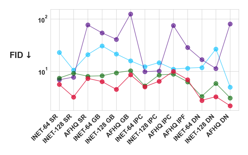
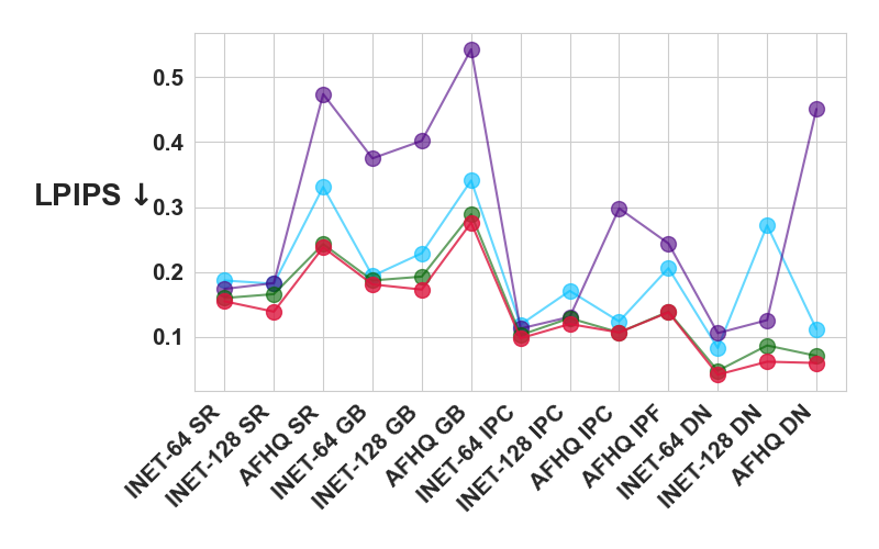
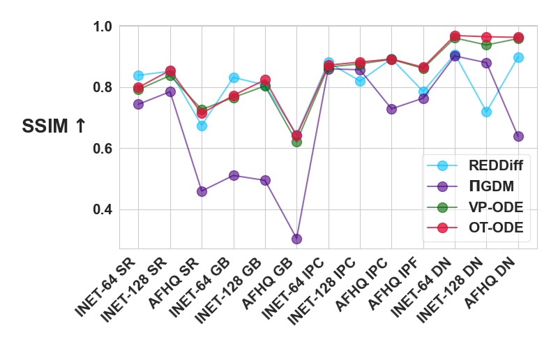
Figure 2: Quantitative evaluation of pretrained VP-SDE model for image inversion on super-resolution (SR), gaussian deblurring (GB), inpainting with centered (IPC) and freeform mask (IPF), and denoising (DN) with $\sigma_{y}=0.05$. We present results on face-blurred ImageNet-64 (INET-64), face-blurred ImageNet-128 (INET-128), and AFHQ.

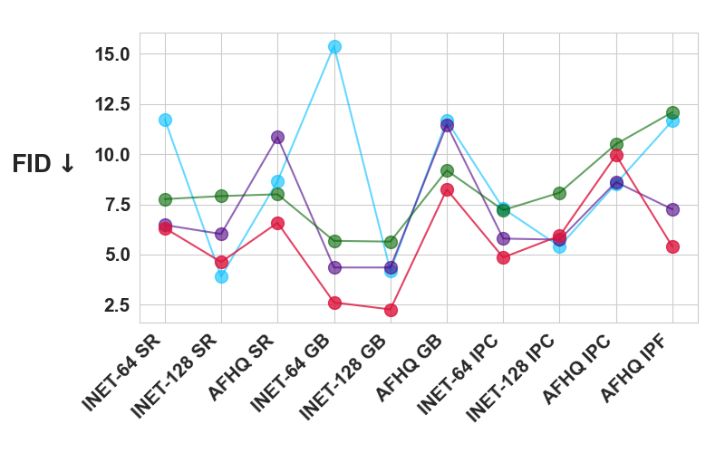
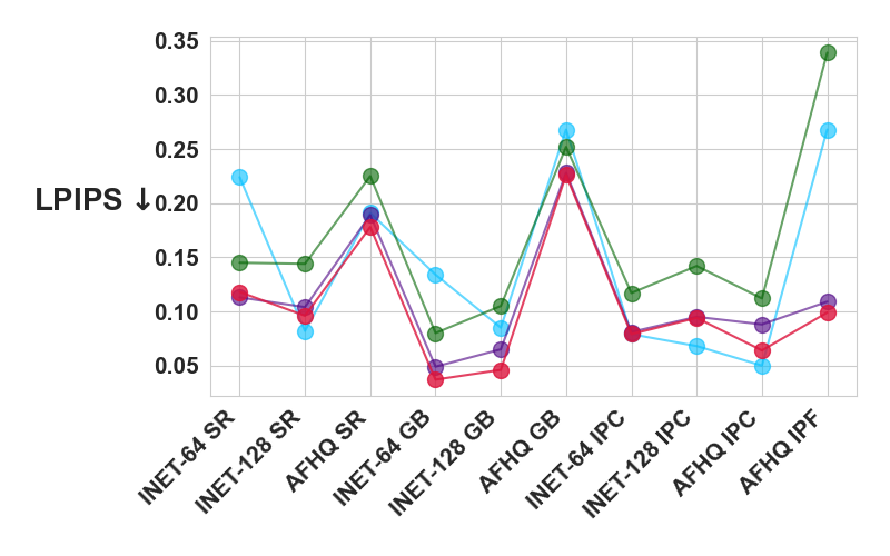
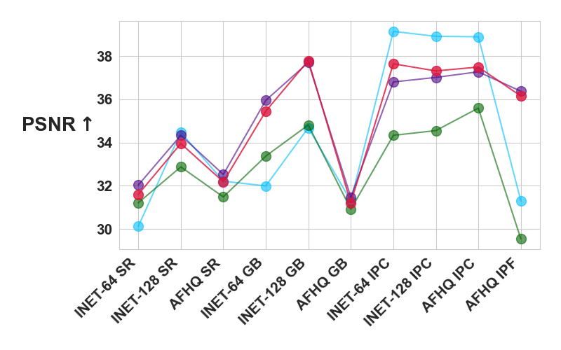
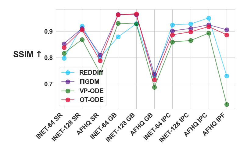
Figure 12: Quantitative evaluation of pretrained VP-SDE model for image inversion on super-resolution (SR), gaussian deblurring (GB), image inpainting - centered mask (IPC) and inpainting - free-form (IPF) with $\sigma_{y}=0$. We show results on face-blurred ImageNet-64 (INET-64), face-blurred ImageNet-128 (INET-128), and AFHQ-256 (AFHQ).

We report quantitative results for the VP-SDE model, across all datasets and linear measurements, in Figure 2 for $\sigma_{y}=0.05$, and in Figure 12 within Sec. D.1 for $\sigma_{y}=0$. Additionally, we report results for the conditional OT flow model in Figure 14 and Figure 13 for $\sigma_{y}=0.05$ and $\sigma_{y}=0$, respectively, in Sec. D.1. Exact numerical values for all the metrics across all datasets and tasks can be found in Appendix D.

Gaussian Deblurring.

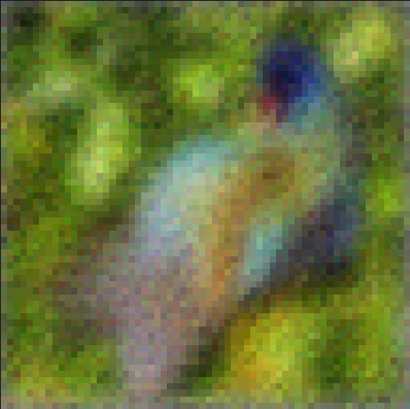
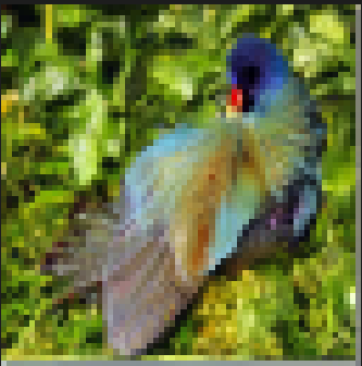
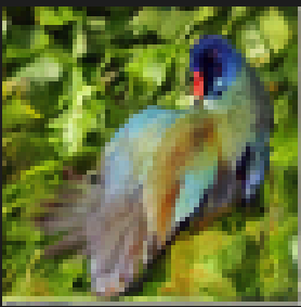
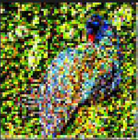
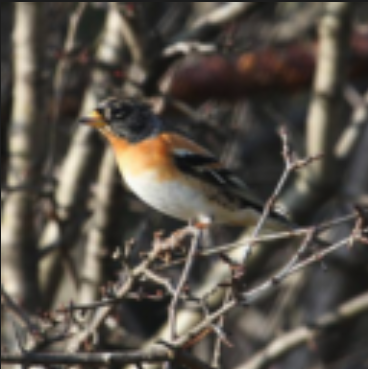
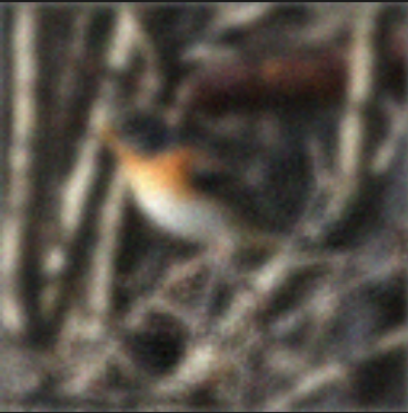
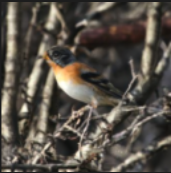
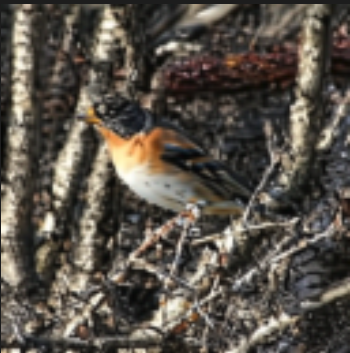
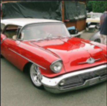
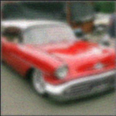
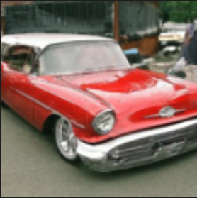
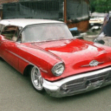
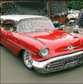
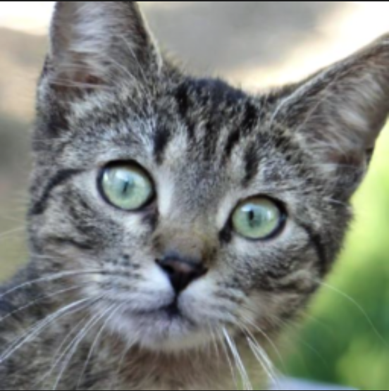
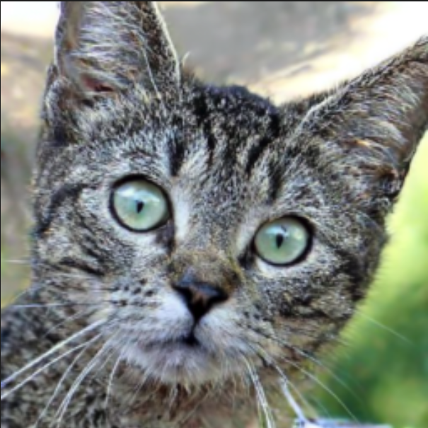
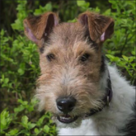
(a) Reference

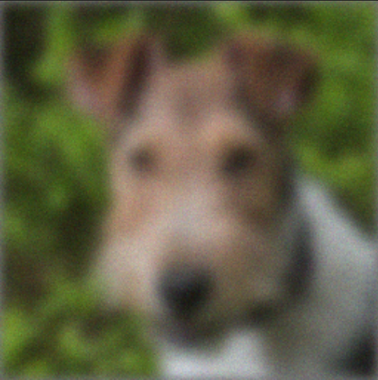
(b) Distorted

(c) OT-ODE

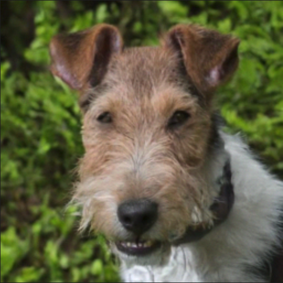
(d) VP-ODE

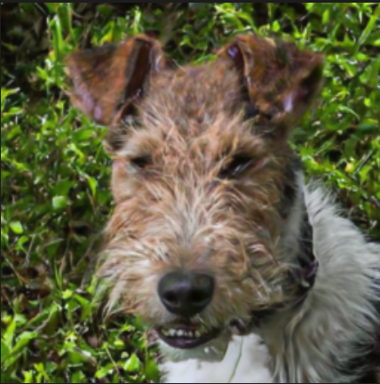
(e) $\Pi$GDM

Figure 15: Image inversion for Gaussian-deblur with conditional OT model and $\sigma_{y}=0.05$ for (first row) ImageNet-64, (second and third row) ImageNet-128, and ( fourth and fifth row) AFHQ.

We report qualitative results for the VP-SDE model in Figure 3 and for the conditional OT flow (cond-OT) model in Figure 15. We observe that for both the VP-SDE model and the cond-OT model, OT-ODE and VP-ODE outperform $\Pi$GDM and RED-Diff, both qualitatively and quantitatively, across all datasets for both $\sigma_{y}=0.05$ and $\sigma_{y}=0$. As shown in Figure 3 and 15, $\Pi$GDM tends to sharpen the images, which sometimes results in unnatural textures in the images. Further, we also observe some unnatural textures and background noise with RED-Diff for $\sigma_{y}=0.05$.

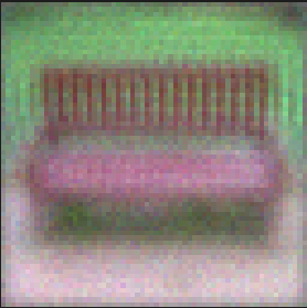
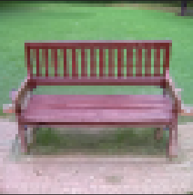
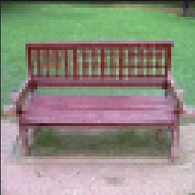
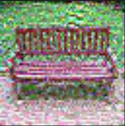
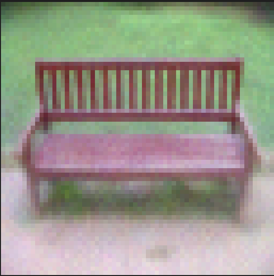
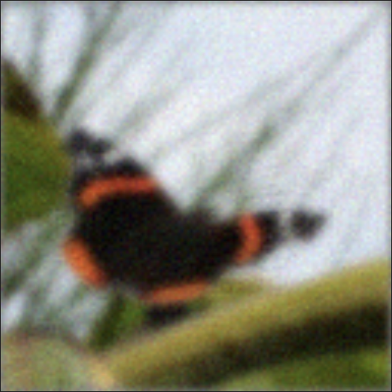
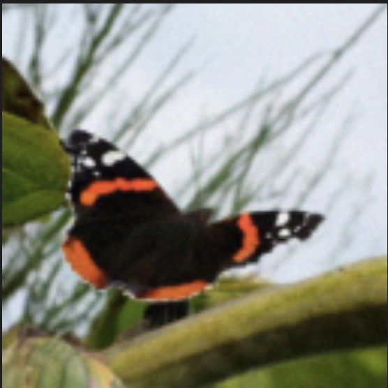
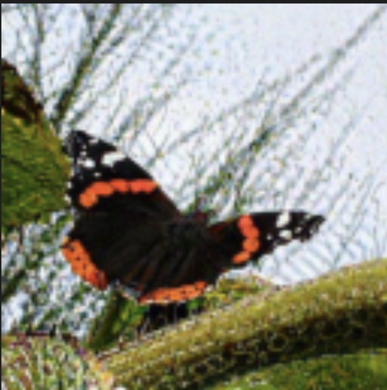
(a) Reference

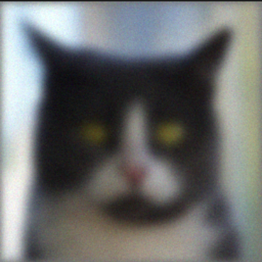
(b) Distorted

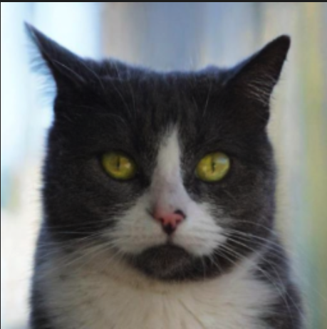
(c) OT-ODE

(d) VP-ODE

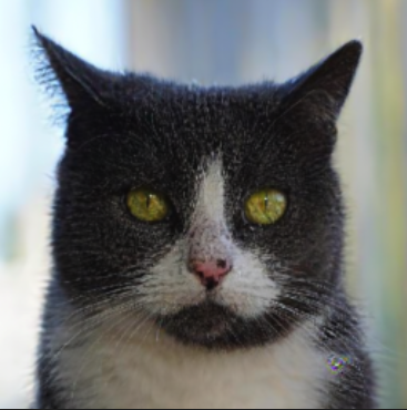
(e) $\Pi$GDM

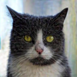
(f) REDDiff

Figure 3: Image inversion for Gaussian deblurring with VP-SDE model and $\sigma_{y}=0.05$ for (first row) ImageNet-64, (second row) ImageNet-128, and (third row) AFHQ.

Super-resolution.

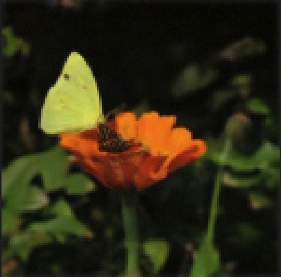
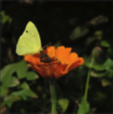
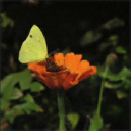
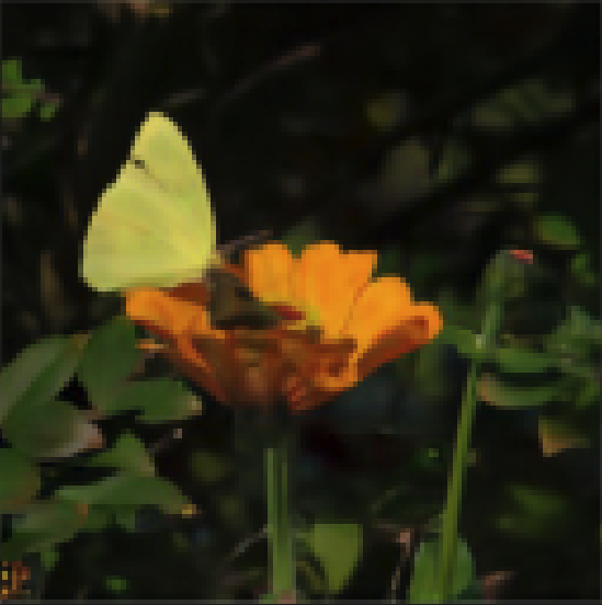
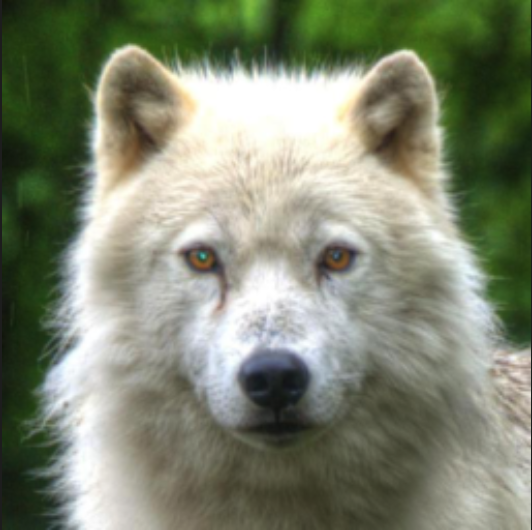
(a) Reference

(b) Distorted

(c) OT-ODE

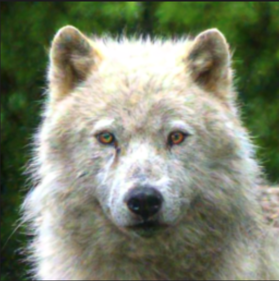
(d) VP-ODE

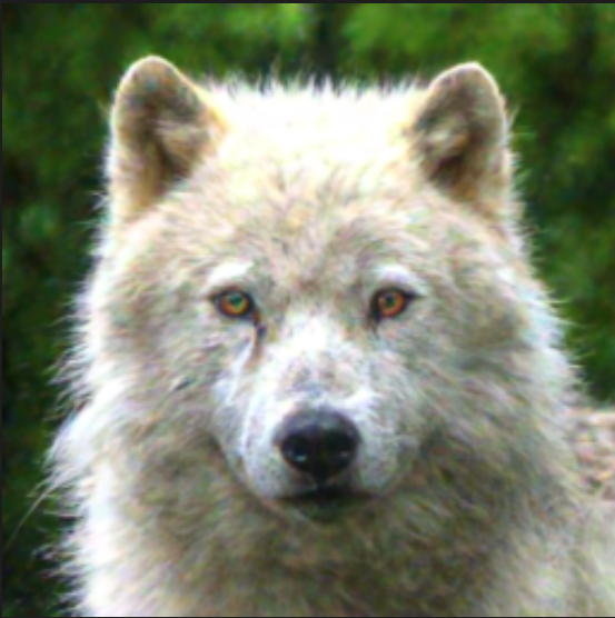
(e) $\Pi$GDM

Figure 16: Image inversion for super-resolution with conditional OT model and $\sigma_{y}=0.05$ for (first row) ImageNet-64 $2\times$, (second row) ImageNet-128 $2\times$, and (third row) AFHQ $4\times$.

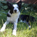
(a) Reference

(b) Distorted

(c) OT-ODE

(d) VP-ODE

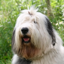
(e) $\Pi$GDM

Figure 22: Image inversion for super-resolution with conditional OT model and $\sigma_{y}=0$ for (first row) ImageNet-64, (second row) ImageNet-128 and (third row) AFHQ.

We report qualitative results for the VP-SDE model in Figure 4 and for the cond-OT model in Figure 16. OT-ODE sampling consistently achieves better FID, LPIPS and PSNR metrics compared to other methods with both VP-SDE model and cond-OT model for $\sigma_{y}=0.05$. Similar to Gaussian deblurring, $\Pi$GDM tends to produce sharper edges. This is certainly desirable to achieve good super-resolution, but sometimes this results in unnatural textures in the images (See Figure 4). RED-Diff for $\sigma_{y}=0.05$ gives slightly blurry images. In our experiments, we observe RED-Diff is sensitive to the values of $\sigma_{y}$, and we get good quality inversion for smaller values of $\sigma_{y}$, but the performance deteriorates with increase in value of $\sigma_{y}$. For noiseless case, as shown in Figure 22 and Figure 25, all the methods achieve comparable performance.

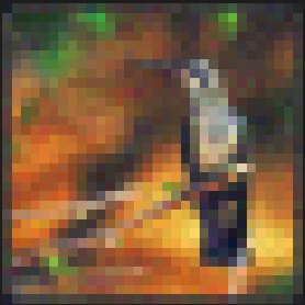
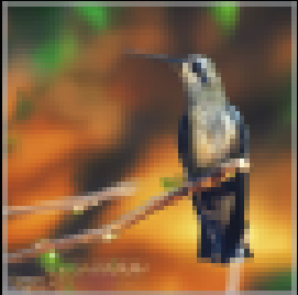
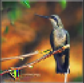
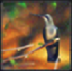
(a) Reference

(b) Distorted

(c) OT-ODE

(d) VP-ODE

(e) $\Pi$GDM

(f) REDDiff

Figure 4: Image inversion for super-resolution with VP-SDE model and $\sigma_{y}=0.05$ for (first row) ImageNet-64 $2\times$, (second row) ImageNet-128 $2\times$, and (third row) AFHQ $4\times$.

Inpainting.

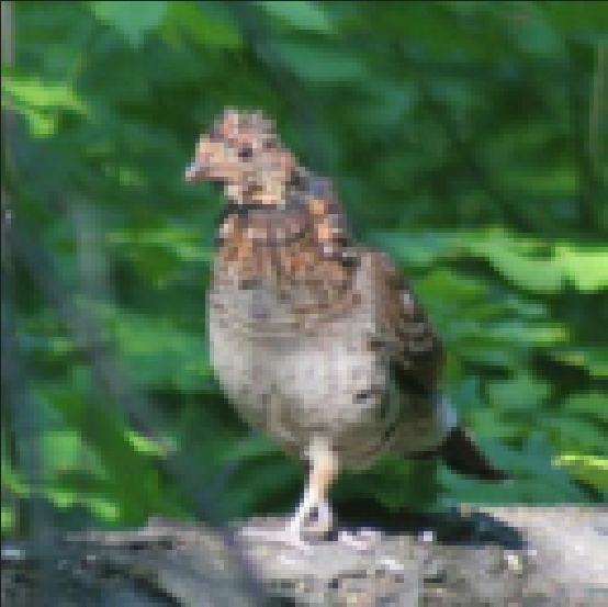
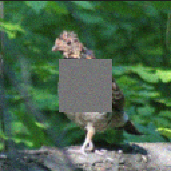
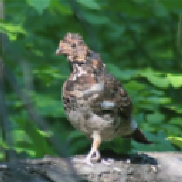
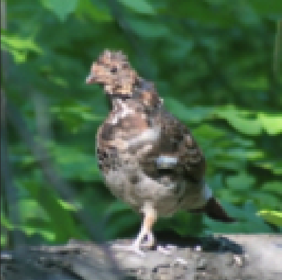
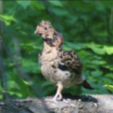
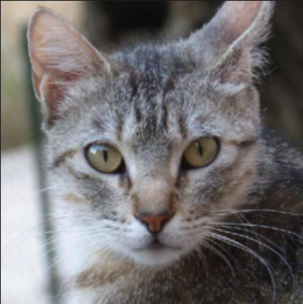
(a) Reference

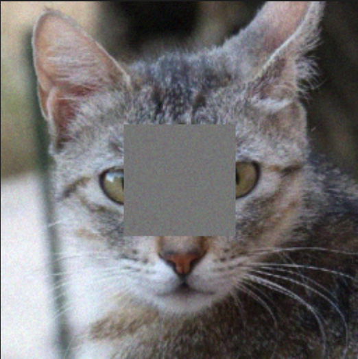
(b) Distorted

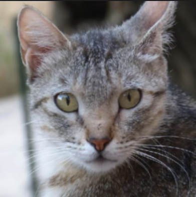
(c) OT-ODE

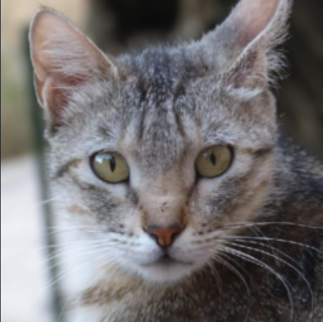
(d) VP-ODE

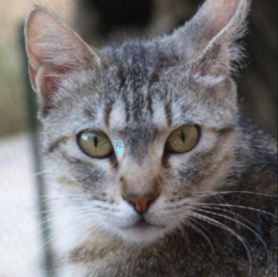
(e) $\Pi$GDM

Figure 17: Image inversion for inpainting (Center mask) with conditional OT model and $\sigma_{y}=0.05$ for (first row) ImageNet-64, (second row) ImageNet-128, and (third row) AFHQ.

For centered mask inpainting, OT-ODE sampling outperforms $\Pi$GDM and RED-Diff in terms of LPIPS, PSNR and SSIM across all datasets at $\sigma_{y}=0.05$ for both the VP-SDE and cond-OT model. Regarding FID, OT-ODE performs comparably to or better than VP-SDE (See Figure 14 and 2). Similar observations hold true for inpainting with freeform mask on AFHQ. We present qualitative results for the VP-SDE model in Figure 5 and the cond-OT model in Figure 17. As evident in these images, OT-ODE sampling results in more semantically meaningful inpainting (for instance, the shape of bird’s neck, and shape of hot-dog bread in Figure 5). In contrast, the inpainted regions generated by RED-Diff tend be blurry and less semantically meaningful. Empirically, we observe that performance of RED-Diff improves as $\sigma_{y}$ decreases. In the noiseless case, RED-Diff achieves higher PSNR and SSIM, but performs worse than OT-ODE in terms of FID and LPIPS (Refer to Figure 12 and 13). Both $\Pi$GDM and OT-ODE achieve similar performance on noiseless inpainting. We further note that noiseless inpainting for OT-ODE can be improved by incorporating null-space decomposition (Wang et al., 2022), which results in improved performance across all datasets. We describe this adjustment in Sec. C.1.

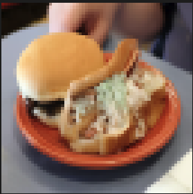
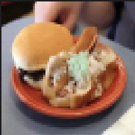
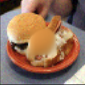
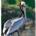
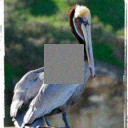
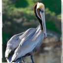
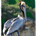
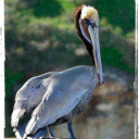
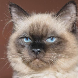
(a) Reference

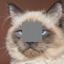
(b) Distorted

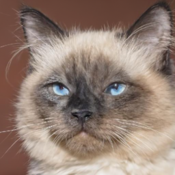
(c) OT-ODE

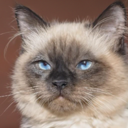
(d) VP-ODE

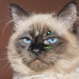
(e) $\Pi$GDM

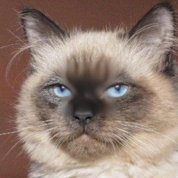
(f) REDDiff

Figure 5: Image inversion for Inpainting (centered mask) with VP-SDE model and $\sigma_{y}=0.05$ for (first row) ImageNet-64, (second row) ImageNet-128, and (third row) AFHQ.

5 Related Work

Training-free noisy linear inversion has been tackled in many ways, often with other solution concepts than posterior sampling (Elad et al., 2023). Utilizing a diffusion model has a host of recent research that we build upon. Our state-of-the-art baselines $\Pi$GDM (Song et al., 2022) and RED-Diff (Mardani et al., 2023) correspond to lines of research in gradient-based corrections and variational inference.

Earlier gradient-based corrections that approximate $\nabla_{{\bm{x}}_{t}}\ln q({\bm{y}}|{\bm{x}}_{t})$ in various ways include Diffusion Posterior Sampling (DPS) (Chung et al., 2022a), Manifold Constrained Gradient (Chung et al., 2022b), and an annealed approximation (Jalal et al., 2021). $\Pi$GDM out-performs earlier methods combining adaptive weights and Gaussian posterior approximation with discrete-time denoising diffusion implicit model (DDIM) sampling (Song et al., 2021a). Here we adapt $\Pi$GDM to all Gaussian probability paths and to flow sampling. Our results show adaptive weights are unnecessary for strongly performing conditional OT flow sampling. Denoising Diffusion Null Models (DDNM) (Wang et al., 2022) proposed an alternative approximation of $\mathbb{E}_{q}[{\bm{x}}_{1}|{\bm{x}}_{t},{\bm{y}}]$ using a null-space decomposition specific to linear inversion, explored in combination with our method in Appendix C.1.

RED-Diff (Mardani et al., 2023) approximates intractable $q({\bm{x}}_{1}|{\bm{y}})$ directly using variational inference, solving for parameters via optimization. RED-Diff was reported to have mode-seeking behavior confirmed by our results where RED-Diff performed better for noiseless inference. Another earlier variational inference method is Denoising Diffusion Restoration Models (DDRM) (Kawar et al., 2022). DDRM showed SVD can be memory-efficient for image applications, and we adapt their SVD implementations for super-resolution and blur. DDRM incorporates noiseless method ILVR Choi et al. (2021), and leverages a measurement-dependent forward process (i.e. $q({\bm{x}}_{t}|{\bm{y}},{\bm{x}}_{1})\neq q({\bm{x}}_{t}|{\bm{x}}_{1})$) like earlier SNIPS (Kawar et al., 2021). SNIPS collapses in special cases to variants proposed in (Song & Ermon, 2019; Song et al., 2021c; Kadkhodaie & Simoncelli, 2020) for linear inversion.

6 Discussion, Limitations, and Future work

We have presented a training-free linear image inversion algorithm using flows that can leverage either pretrained diffusion or flow models. The algorithm is simple, stable, and requires no hyperparameter tuning when used with conditional OT probability paths. Our method combines past ideas from diffusion including $\Pi$GDM and early starting with the conditional OT probability path from flows, and our results demonstrate that this combination provides high quality image inversion for both noisy and noiseless tasks across a variety of datasets. Our algorithm using the conditional OT path (OT-ODE) produced results superior to the VP path (VP-ODE) and also to $\Pi$GDM and REDDiff for noisy inversion. For noiseless inversion, the perceptual quality from OT-ODE is on par with $\Pi$GDM.

One important limitation, shared with most past related research, is a restriction to linear observations with scalar variance. Our method can extend to arbitrary covariance, but non-linear observations are more complex. Non-linear observations occur with image inversion tasks when utilizing latent, not pixel-space, diffusion or flow models. Applying our approach to such measurements requires devising an alternative $q^{app}({\bm{y}}|{\bm{x}}_{t})$. Another shared limitation is that we consider the non-blind setting with known ${\bm{A}}$ and $\sigma_{y}$.

Future research could tackle these limitations. For non-linear observations, we could perhaps build upon (Rout et al., 2023) that uses a latent diffusion model for linear inversion. For the blind setting, we might start from blind extensions to DPS and DDRM (Chung et al., 2023; Murata et al., 2023). As demonstrated here, we may be able to adapt and possibly improve these approaches via conversion to flow sampling using conditional OT paths.

Appendix A Proofs

For clarity, we restate Theorems and Lemmas from the main text before giving their proof.

[conversion]

Appendix B Our method for any Gaussian probability path

Algorithm 1 in the main text is specific to conditional OT probability paths. Here we provide Algorithm 2 for any Gaussian probability path specified by Eq. 5. Algorithm 1 and Algorithm 2 are written assuming a denoiser $\widehat{{\bm{x}}_{1}}({\bm{x}}_{t})$ is provided from a pretrained diffusion model. For completeness, we also include equivalent Algorithm 3 that assumes $\widehat{{\bm{v}}}({\bm{x}}_{t})$ is provided from a pretrained flow model. In all cases, the vector field or denoiser is evaluated only once per iteration.

Our VP-ODE sampling results correspond to $\alpha_{t}$ and $\sigma_{t}$ given from the Variance-Preserving path, which can be found in (Lipman et al., 2022).

Algorithm 2 Training-free image inversion via flows with given pre-trained denoiser

1:Pretrained denoiser $\widehat{{\bm{x}}_{1}}({\bm{x}}_{t})$ converted to Gaussian probability path with $\alpha_{t}$ and $\sigma_{t}$ using Section 3.1, noisy measurement ${\bm{y}}$, measurement matrix ${\bm{A}}$, initial time $t$, adaptive weights $\gamma_{t}$, and std $\sigma_{y}$

2:Initialize ${\bm{x}}_{t}=\alpha_{t}{\mathbf{y}}+\sigma_{t}\epsilon$, where $\epsilon\sim\mathcal{N}(0,{\bm{I}})$ $\triangleright$ Initialize ${\bm{x}}_{t}$, Eq. 17

3:${\bm{z}}_{t}={\bm{x}}_{t}$

4:for each time step $t^{\prime}$ of ODE integration do $\triangleright$ Integrate ODE from $t^{\prime}=t$ to $1$.

5:     $r_{t^{\prime}}^{2}=\frac{\sigma_{t^{\prime}}^{2}}{\sigma_{t^{\prime}}^{2}+\alpha_{t^{\prime}}^{2}}$ $\triangleright$ Value of $r_{t}^{2}$ from Eq. 16

6:     $\widehat{{\bm{v}}}=\left(\alpha_{t}\frac{d\ln(\alpha_{t}/\sigma_{t})}{dt}\right)\widehat{{\bm{x}}_{1}}+\frac{d\ln\sigma_{t}}{dt}{\bm{z}}_{t}$ $\triangleright$ Convert $\widehat{{\bm{x}}_{1}}$ to vector field, Eq. 10

7:     ${\bm{g}}=({\bm{y}}-{\bm{A}}\widehat{{\bm{x}}_{1}})^{\top}(r_{t^{\prime}}^{2}{\bm{A}}{\bm{A}}^{\top}+\sigma_{y}^{2}{\bm{I}})^{-1}{\bm{A}}\frac{\partial\widehat{{\bm{x}}_{1}}}{\partial{\bm{z}}_{t^{\prime}}}$ $\triangleright$ $\Pi$GDM correction

8:     $\widehat{{\bm{v}}}_{\text{corrected}}=\widehat{{\bm{v}}}+\sigma_{t}^{2}\frac{d\ln(\alpha_{t}/\sigma_{t})}{dt}\gamma_{t}{\bm{g}}$ $\triangleright$ Correct unconditional vector field $\widehat{{\bm{v}}}$, Eq. 15

9:end for

Algorithm 3 Training-free image inversion via flows with given pre-trained vector field

1:Pretrained vector field $\widehat{{\bm{v}}}({\bm{x}}_{t})$ converted to Gaussian probability path with $\alpha_{t}$ and $\sigma_{t}$ using Section 3.1, noisy measurement ${\bm{y}}$, measurement matrix ${\bm{A}}$, initial time $t$, adaptive weights $\gamma_{t}$, and std $\sigma_{y}$

2:Initialize ${\bm{x}}_{t}=\alpha_{t}{\mathbf{y}}+\sigma_{t}\epsilon$, where $\epsilon\sim\mathcal{N}(0,{\bm{I}})$ $\triangleright$ Initialize ${\bm{x}}_{t}$, Eq. 17

3:${\bm{z}}_{t}={\bm{x}}_{t}$

4:for each time step $t^{\prime}$ of ODE integration do $\triangleright$ Integrate ODE from $t^{\prime}=t$ to $1$.

5:     $\widehat{{\bm{v}}}=\widehat{{\bm{v}}}({\bm{z}}_{t^{\prime}})$ $\triangleright$ ${\bm{z}}_{t^{\prime}}$ is value of ${\bm{x}}_{t}$ at time $t^{\prime}$ during ODE integration

6:     $r_{t^{\prime}}^{2}=\frac{\sigma_{t^{\prime}}^{2}}{\sigma_{t^{\prime}}^{2}+\alpha_{t^{\prime}}^{2}}$ $\triangleright$ Value of $r_{t}^{2}$ from Eq. 16

7:     $\widehat{{\bm{x}}_{1}}=\left(\alpha_{t}\frac{d\ln(\alpha_{t}/\sigma_{t})}{dt}\right)^{-1}\left(\widehat{{\bm{v}}}-\frac{d\ln\sigma_{t}}{dt}{\bm{z}}_{t}\right)$ $\triangleright$ Convert vector field to $\widehat{{\bm{x}}_{1}}$, Eq. 10

8:     ${\bm{g}}=({\bm{y}}-{\bm{A}}\widehat{{\bm{x}}_{1}})^{\top}(r_{t^{\prime}}^{2}{\bm{A}}{\bm{A}}^{\top}+\sigma_{y}^{2}{\bm{I}})^{-1}{\bm{A}}\frac{\partial\widehat{{\bm{x}}_{1}}}{\partial{\bm{z}}_{t^{\prime}}}$ $\triangleright$ $\Pi$GDM correction

9:     $\widehat{{\bm{v}}}_{\text{corrected}}=\widehat{{\bm{v}}}+\sigma_{t}^{2}\frac{d\ln(\alpha_{t}/\sigma_{t})}{dt}\gamma_{t}{\bm{g}}$ $\triangleright$ Correct unconditional vector field $\widehat{{\bm{v}}}$, Eq. 15

10:end for

Appendix C Ablation Study

Choice of initialization.

We initialize the flow at time $t>0$ as ${\bm{x}}_{t}=\alpha_{t}{\bm{y}}+\sigma_{t}\epsilon$ (y-init) where $\epsilon\sim\mathcal{N}(0,{\bm{I}})$. Another choice of initialization is to use ${\bm{x}}_{t}=\alpha_{t}{\bm{A}}^{\dagger}{\bm{y}}+\sigma_{t}\epsilon$. However, empirically we find that this initialization performs worse that y-init on cond-OT model with OT-ODE sampling. We summarize the results of our ablation study in Table 1. We find that on Gaussian deblurring, initialization with ${\bm{A}}^{\dagger}{\bm{y}}$ does worse than y-init, while the performance of both the initializations is comparable for super-resolution. In all our experiments, we use y-init, due to its better performance on Gaussian deblurring.

Table 1: Quantitative evaluation of choice of initialization for conditional OT flow model with OT-ODE sampling on AFHQ dataset. We find that y-init outperforms ${\bm{A}}^{\dagger}{\bm{y}}$ on Gaussian deblurring.

Initialization	Start time	NFEs $\downarrow$	Gaussian deblur, $\sigma_{y}=0.05$				SR 4$\times$, $\sigma_{y}=0.05$
			FID $\downarrow$	LPIPS $\downarrow$	PSNR $\uparrow$	SSIM $\uparrow$	FID $\downarrow$	LPIPS $\downarrow$	PSNR $\uparrow$	SSIM $\uparrow$
y init	0.2	100	7.57	0.268	30.28	0.626	6.03	0.219	31.12	0.739
${\bm{A}}^{\dagger}{\bm{y}}$	0.1	100	41.22	0.449	28.79	0.392	12.93	0.292	30.46	0.664
${\bm{A}}^{\dagger}{\bm{y}}$	0.2	100	56.42	0.554	28.11	0.249	6.09	0.219	31.12	0.739

Ablation over $\gamma_{t}$ for VP-ODE sampling.

We compare the performance of $\gamma_{t}=1$ against $\gamma_{t}=\sqrt{\frac{\alpha_{t}}{\alpha_{t}^{2}+\sigma_{t}^{2}}}$. We show results of VP-ODE sampling with VP-SDE model in Table 2 and Table 3. As seen our choice of $\gamma_{t}$ outperform $\gamma_{t}=1$ across all the metrics on face-blurred ImageNet-128.

Table 2: Quantitative evaluation of value of $\gamma_{t}$ in VP-ODE sampling with VP-SDE model on face-blurred ImageNet-$128$ dataset.

$\gamma_{t}$	Start time	NFEs $\downarrow$	SR 2$\times$, $\sigma_{y}=0.05$				Gaussian deblur, $\sigma_{y}=0.05$
			FID $\downarrow$	LPIPS $\downarrow$	PSNR $\uparrow$	SSIM $\uparrow$	FID $\downarrow$	LPIPS $\downarrow$	PSNR $\uparrow$	SSIM $\uparrow$
$1$	0.4	60	32.66	0.371	29.06	0.530	29.31	0.346	29.12	0.554
$\sqrt{\frac{\alpha_{t}}{\alpha_{t}^{2}+\sigma_{t}^{2}}}$	0.4	60	9.14	0.167	32.06	0.838	10.14	0.196	31.59	0.800

Table 3: Quantitative evaluation of value of $\gamma_{t}$ in VP-ODE sampling with VP-SDE model on face-blurred ImageNet-$128$ dataset.

$\gamma_{t}$	Start time	NFEs $\downarrow$	Inpainting-Center, $\sigma_{y}=0.05$				Denoising, $\sigma_{y}=0.05$
			FID $\downarrow$	LPIPS $\downarrow$	PSNR $\uparrow$	SSIM $\uparrow$	FID $\downarrow$	LPIPS $\downarrow$	PSNR $\uparrow$	SSIM $\uparrow$
$1$	0.3	70	53.03	0.285	31.55	0.737	28.37	0.238	31.63	0.786
$\sqrt{\frac{\alpha_{t}}{\alpha_{t}^{2}+\sigma_{t}^{2}}}$	0.3	70	8.47	0.129	34.43	0.876	5.83	0.087	35.85	0.938

Variation of performance with NFEs.

We analyze the variation in performance of OT-ODE, VP-ODE and $\Pi$GDM linear inversion procedures as NFEs are varied. The results have been summarized in Figure 6. We observe that OT-ODE consistently outperforms VP-ODE and $\Pi$GDM across all measurements in terms of FID and LPIPS metrics, even for NFEs as small as $20$. We also note that the choice of starting time matters to achieve good performance with OT-ODE. For instance, starting at $t=0.4$ outperforms $t=0.2$ when NFEs are small, but eventually as NFEs is increased, $t=0.2$ performs better. We also note that $\Pi$GDM achieves higher values of PSNR and SSIM at smaller NFEs for super-resolution but has inferior FID and LPIPS compared to OT-ODE linear inversion.

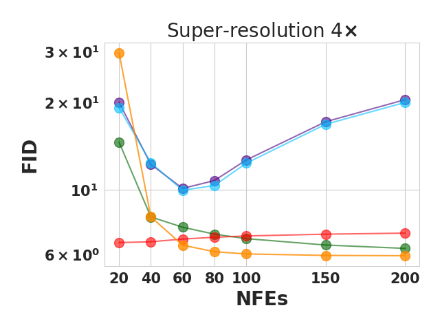
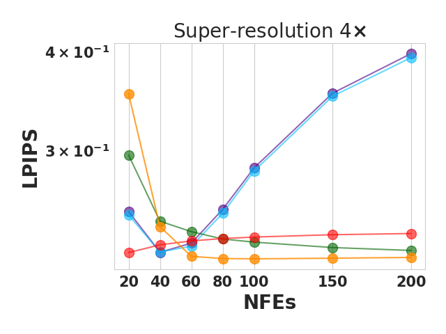
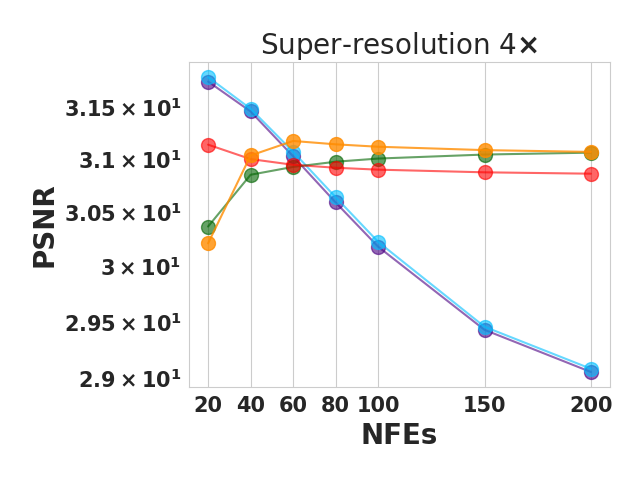
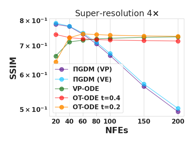
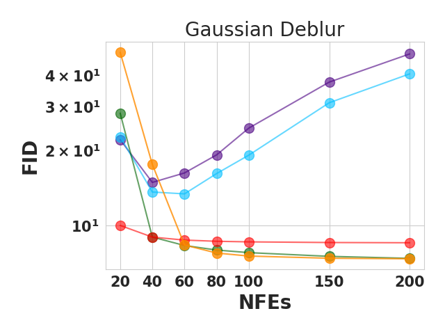
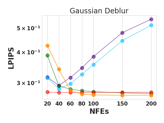
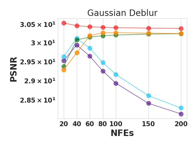
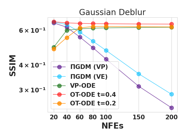
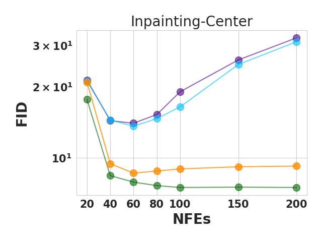
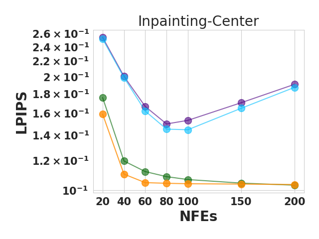
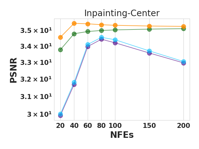
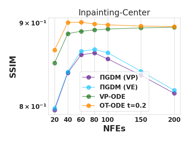
Figure 6: Performance of different linear inversion procedures with variation in NFEs on AFHQ dataset. We use pretrained conditional OT model and set $\sigma_{y}=0.05$. The legends VP and VE indicate the choice of $r_{t}^{2}$ used in $\Pi$GDM (See Sec. E.1). Time $t=0.2$ and $0.4$ indicates the starting time of sampling with OT-ODE.

Choice of starting time.

We plot the variation in performance of OT-ODE and VP-ODE sampling with change in start times for conditional OT model and VP-SDE model on AFHQ dataset in Figure 7 and Figure 8, respectively. We note that in general, OT-ODE sampling achieves optimal performance across all measurements and all metrics at $t=0.2$ while VP-ODE sampling achieves optimal performance between start times of $t=0.3$ and $0.4$. In this work, for all the experiments, we use $t=0.2$ for OT-ODE sampling and $t=0.4$ for VP-ODE sampling.

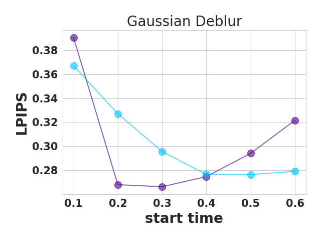
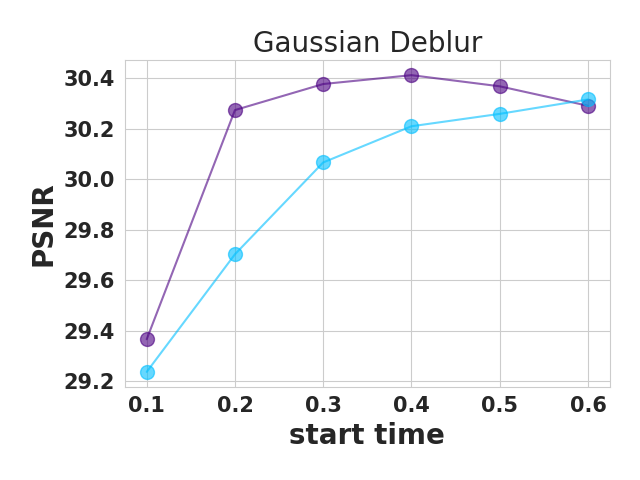
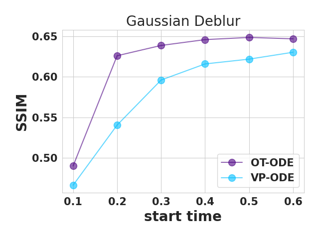
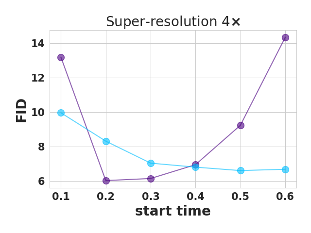
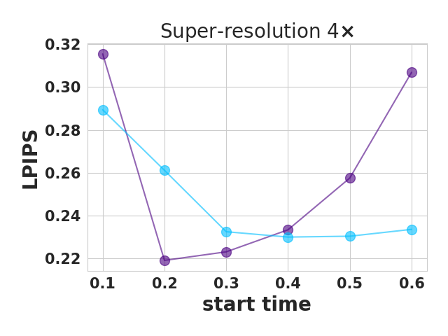
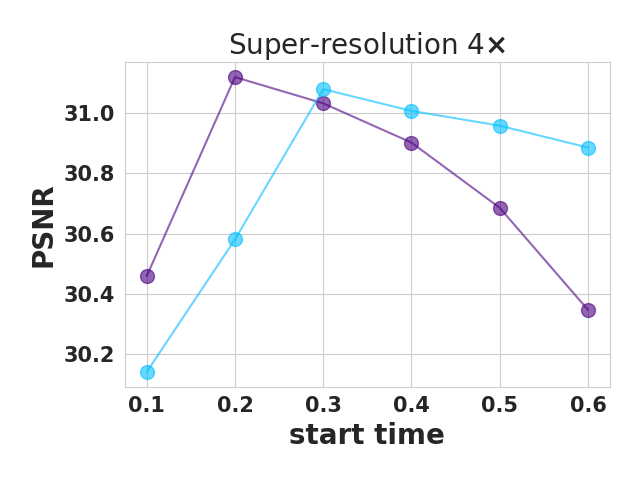
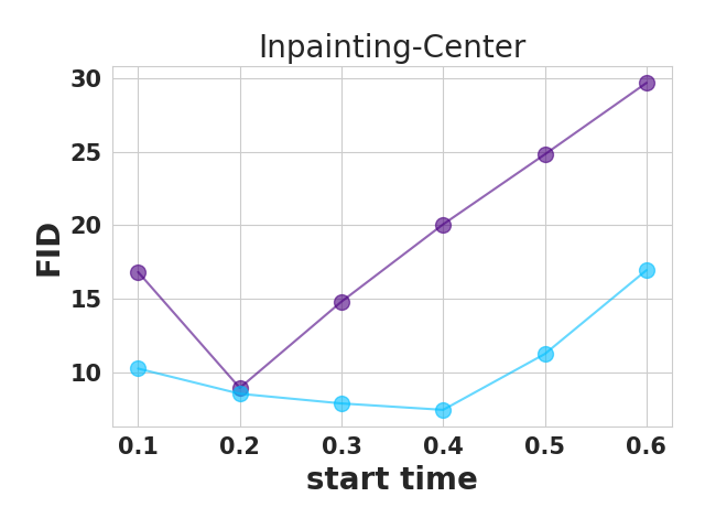
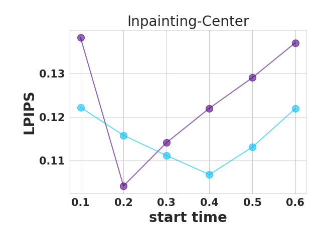
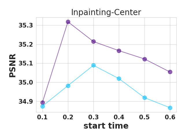
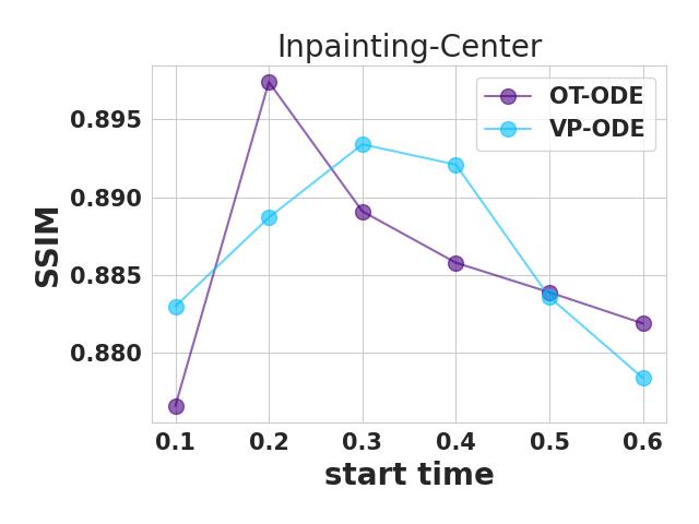
Figure 7: Performance of OT and VP-ODE sampling with variation in start times on AFHQ dataset. We use pretrained cond-OT model and set $\sigma_{y}=0.05$.

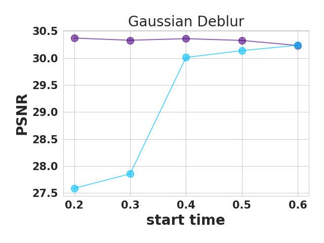
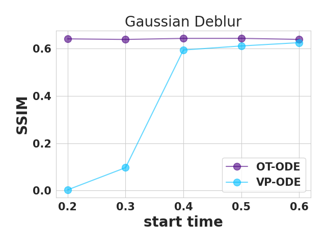
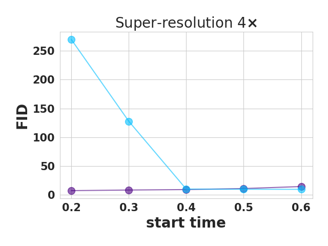
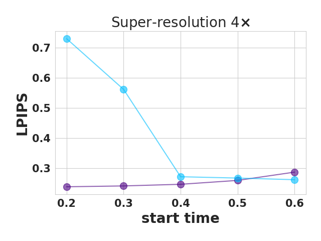
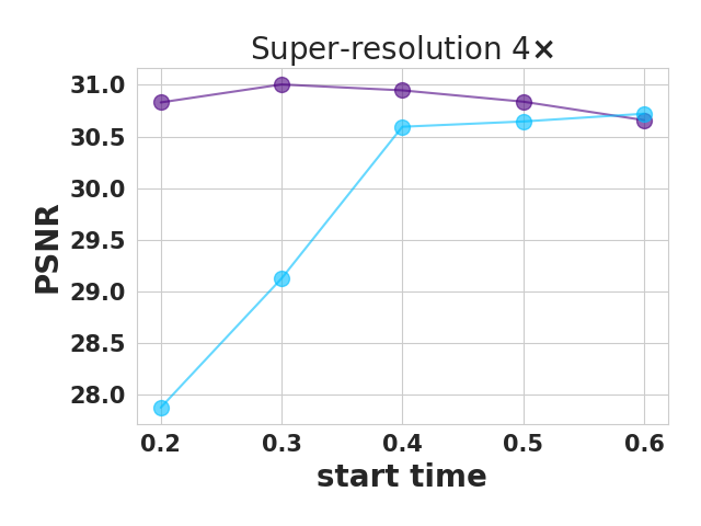
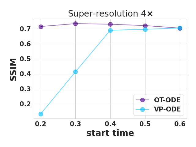
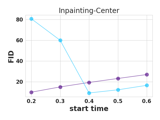
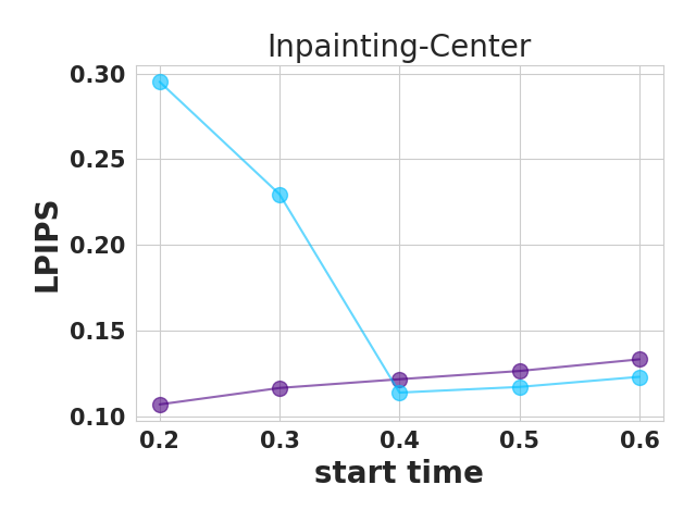
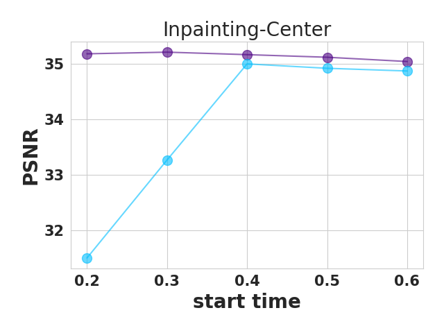
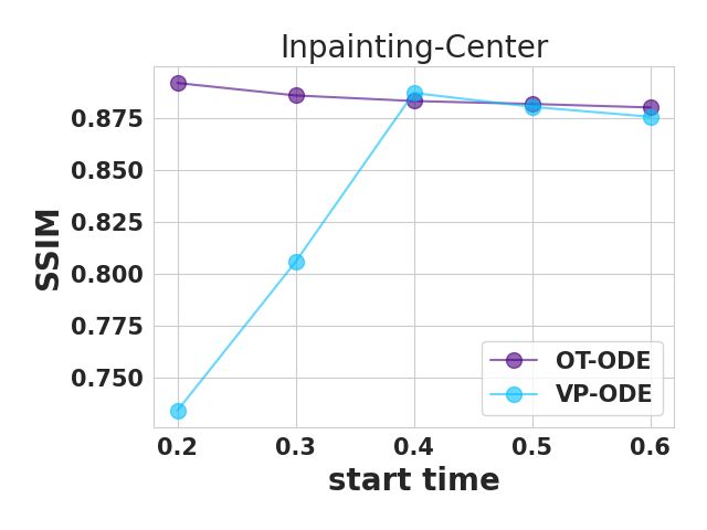
Figure 8: Performance of OT and VP-ODE sampling with variation in start times on AFHQ dataset. We use pretrained VP-SDE model and set $\sigma_{y}=0.05$.

C.1 Noiseless null and range space decomposition

When $\sigma_{y}^{2}=0$, we can produce a vector field approximation with even lower Conditional Flow Matching loss by applying a null-space and range-space decomposition motivated by DDNM (Wang et al., 2022). In particular, when ${\bm{y}}={\bm{A}}{\bm{x}}_{1}$, we have that ${\bm{A}}^{\dagger}{\bm{y}}={\bm{A}}^{\dagger}{\bm{A}}{\bm{x}}_{1}$ (where ${\bm{A}}^{\dagger}$ is the pseudo-inverse of ${\bm{A}}$) and so

$$\mathbb{E}_{q}[{\bm{x}}_{1}|{\bm{x}}_{t},{\bm{y}}]=\mathbb{E}_{q}[{\bm{A}}^{\dagger}{\bm{A}}{\bm{x}}_{1}+({\bm{I}}-{\bm{A}}^{\dagger}{\bm{A}}){\bm{x}}_{1}|{\bm{x}}_{t},{\bm{y}}]={\bm{A}}^{\dagger}{\bm{y}}+({\bm{I}}-{\bm{A}}^{\dagger}{\bm{A}})\mathbb{E}_{q}[{\bm{x}}_{1}|{\bm{x}}_{t},{\bm{y}}].$$ (18)

So when $\sigma_{\bm{y}}^{2}=0$, it is only necessary to approximate the second term, as the first term is known through ${\bm{y}}$. The regression loss is minimized for the first term automatically and $\widehat{{\bm{x}}_{1}}({\bm{x}}_{t},{\bm{y}})$ is only responsible for predicting the second term.

In our experiments, we find that null space decomposition helps in inpainting but not other measurements. We summarize the results in Table 4, 5, 7, 6, 8 and 9.

Table 4: Comparison of performance OT-ODE sampling and OT-ODE sampling with null and range space decomposition (NRSD) on face-blurred ImageNet-$64\times 64$. For inpainting, OT-ODE sampling with null and range space decomposition outperforms simple OT-ODE sampling.

Model	Inference	NFEs $\downarrow$	Inpainting-Center, $\sigma_{y}=0$
			FID $\downarrow$	LPIPS $\downarrow$	PSNR $\uparrow$	SSIM $\uparrow$
OT	OT-ODE	80	4.94	0.080	37.42	0.885
OT	OT-ODE-NRSD	80	3.84	0.072	38.23	0.888
OT	VP-ODE	80	7.85	0.120	34.24	0.858
VP-SDE	OT-ODE	80	4.85	0.079	37.64	0.887
VP-SDE	OT-ODE-NRSD	80	3.77	0.072	38.24	0.888
VP-SDE	VP-ODE	80	7.21	0.117	34.33	0.860

Table 5: Comparison of performance OT-ODE sampling and OT-ODE sampling with null and range space decomposition (NRSD) on face-blurred ImageNet-$64\times 64$. For tasks like super-resolution and Gaussian deblurring, OT-ODE sampling without null and range space decomposition outperforms other methods.

Model	Inference	NFEs $\downarrow$	SR 2$\times$, $\sigma_{y}=0$				Gaussian deblur, $\sigma_{y}=0$
			FID $\downarrow$	LPIPS $\downarrow$	PSNR $\uparrow$	SSIM $\uparrow$	FID $\downarrow$	LPIPS $\downarrow$	PSNR $\uparrow$	SSIM $\uparrow$
OT	OT-ODE	80	6.46	0.119	31.59	0.839	2.59	0.038	35.31	0.961
OT	OT-ODE-NRSD	80	7.37	0.134	31.05	0.799	3.05	0.044	35.19	0.956
OT	VP-ODE	80	8.29	0.147	31.20	0.817	6.13	0.083	33.31	0.929
VP-SDE	OT-ODE	80	6.32	0.118	31.60	0.839	2.61	0.037	35.45	0.963
VP-SDE	OT-ODE-NRSD	80	7.13	0.133	31.06	0.798	2.99	0.044	35.24	0.956
VP-SDE	VP-ODE	80	7.76	0.145	31.21	0.817	5.68	0.080	33.37	0.931

Table 6: Comparison of performance OT-ODE sampling and OT-ODE sampling with null and range space decomposition (NRSD) on face-blurred ImageNet-$128\times 128$.

Model	Inference	NFEs $\downarrow$	SR 2$\times$, $\sigma_{y}=0$				Gaussian deblur, $\sigma_{y}=0$
			FID $\downarrow$	LPIPS $\downarrow$	PSNR $\uparrow$	SSIM $\uparrow$	FID $\downarrow$	LPIPS $\downarrow$	PSNR $\uparrow$	SSIM $\uparrow$
OT	OT-ODE	70	4.46	0.097	33.88	0.903	2.09	0.048	37.49	0.961
OT	OT-ODE-NRSD	70	3.62	0.099	33.24	0.876	1.42	0.036	38.35	0.969
OT	VP-ODE	70	7.69	0.144	32.93	0.871	6.02	0.108	34.73	0.925
VP-SDE	OT-ODE	70	4.62	0.096	33.95	0.906	2.26	0.046	37.79	0.967
VP-SDE	OT-ODE-NRSD	70	3.44	0.098	33.28	0.877	1.36	0.035	38.44	0.969
VP-SDE	VP-ODE	70	7.91	0.144	32.87	0.869	5.64	0.105	34.81	0.928

Table 7: Comparison of performance OT-ODE sampling and OT-ODE sampling with null and range space decomposition (NRSD) on face-blurred ImageNet-$128\times 128$

Model	Inference	NFEs $\downarrow$	Inpainting-Center, $\sigma_{y}=0$
			FID $\downarrow$	LPIPS $\downarrow$	PSNR $\uparrow$	SSIM $\uparrow$
OT	OT-ODE	70	5.88	0.095	37.06	0.894
OT	OT-ODE-NRSD	70	3.95	0.074	38.27	0.906
OT	VP-ODE	70	8.63	0.144	34.48	0.864
VP-SDE	OT-ODE	70	5.93	0.094	37.31	0.898
VP-SDE	OT-ODE-NRSD	70	3.84	0.073	38.27	0.906
VP-SDE	VP-ODE	70	8.08	0.142	34.55	0.865

Table 8: Comparison of performance OT-ODE sampling and OT-ODE sampling with null and range space decomposition (NRSD) on AFHQ-$256\times 256$

Model	Inference	NFEs $\downarrow$	SR 4$\times$, $\sigma_{y}=0$				Gaussian deblur, $\sigma_{y}=0$
			FID $\downarrow$	LPIPS $\downarrow$	PSNR $\uparrow$	SSIM $\uparrow$	FID $\downarrow$	LPIPS $\downarrow$	PSNR $\uparrow$	SSIM $\uparrow$
OT	OT-ODE	100	5.75	0.169	32.25	0.792	6.63	0.213	31.29	0.722
OT	OT-ODE-NRSD	100	5.73	0.179	31.69	0.753	7.32	0.237	30.72	0.665
OT	VP-ODE	100	6.14	0.194	31.93	0.773	7.38	0.231	31.10	0.705
VP-SDE	OT-ODE	100	6.58	0.178	32.18	0.789	8.24	0.226	31.21	0.717
VP-SDE	OT-ODE-NRSD	100	6.99	0.195	31.65	0.752	10.19	0.255	30.66	0.662
VP-SDE	VP-ODE	100	8.00	0.225	31.48	0.742	9.19	0.252	30.91	0.688

Table 9: Comparison of performance OT-ODE sampling and OT-ODE sampling with null and range space decomposition (NRSD) on AFHQ-$256\times 256$

Model	Inference	NFEs $\downarrow$	Inpainting-Center, $\sigma_{y}=0$				Inpainting-Free-form, $\sigma_{y}=0$
			FID $\downarrow$	LPIPS $\downarrow$	PSNR $\uparrow$	SSIM $\uparrow$	FID $\downarrow$	LPIPS $\downarrow$	PSNR $\uparrow$	SSIM $\uparrow$
OT	OT-ODE	100	8.87	0.061	37.45	0.921	4.98	0.097	36.15	0.889
OT	OT-ODE-NRSD	100	7.95	0.046	38.01	0.921	4.12	0.083	36.62	0.890
OT	VP-ODE	100	9.18	0.106	35.63	0.898	6.92	0.135	34.72	0.869
VP-SDE	OT-ODE	100	9.95	0.064	37.49	0.918	5.39	0.099	36.15	0.887
VP-SDE	OT-ODE-NRSD	100	10.96	0.052	37.95	0.916	4.87	0.089	36.52	0.884
VP-SDE	VP-ODE	100	10.50	0.112	35.59	0.893	7.36	0.139	34.65	0.865

(a) Reference

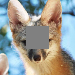
(b) Distorted

(c) OT-ODE

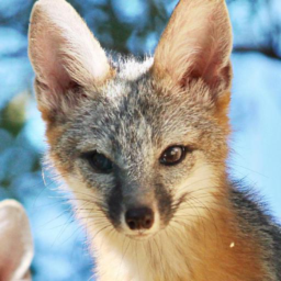
(d) OT-ODE-NRSD

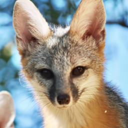
(e) $\Pi$GDM

Figure 9: Comparison of inpainting (center mask) via OT-ODE sampling with and without null and range space decomposition (NRSD). We use conditional OT model and $\sigma_{y}=0$ for (first and second row) face-blurred ImageNet-64, (third row) face-blurred ImageNet-128, and (fourth row) AFHQ.

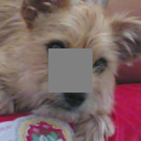
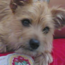
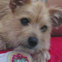
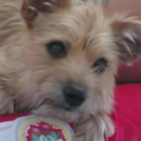
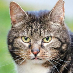
(a) Reference

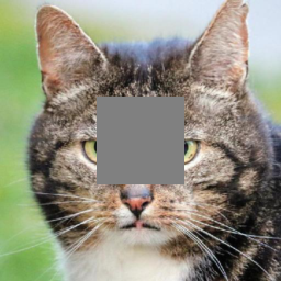
(b) Distorted

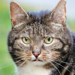
(c) OT-ODE

(d) OT-ODE-NRSD

(e) $\Pi$GDM

Figure 10: Comparison of inpainting (center mask) via OT-ODE sampling with and without null and range space decomposition (NRSD) for (first row) face-blurred ImageNet-64, (second row) face-blurred ImageNet-128, and (third row) AFHQ. We use VP-SDE model and $\sigma_{y}=0$.

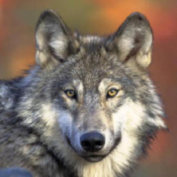
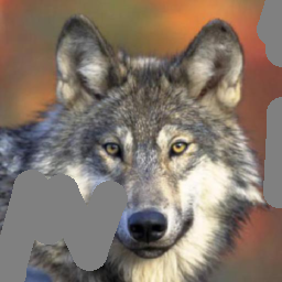
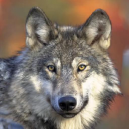
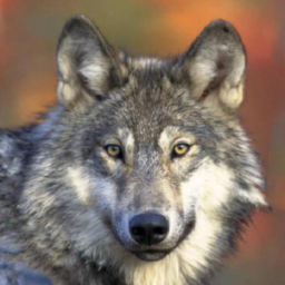
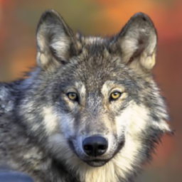
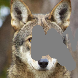
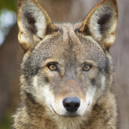
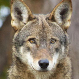
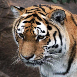
(a) Reference

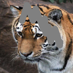
(b) Distorted

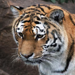
(c) OT-ODE

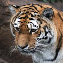
(d) OT-ODE-NRSD

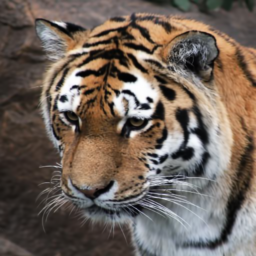
(e) $\Pi$GDM

Figure 11: Comparison of inpainting (free-form mask) via OT-ODE sampling with and without null and range space decomposition (NRSD) for AFHQ. We use conditional OT model and $\sigma_{y}=0$.

Appendix D Additional Empirical Results

D.1 Figures for conditional OT flow matching model

The main text includes figures produced with the denoiser from the continuous-time VP-SDE diffusion model. Here we provide the same figures using our pre-trained conditional OT flow matching model using Algorithm 3 instead. To save compute, here we only include our $\Pi$GDM baseline as REDDiff required extensive hyperparameter tuning. The qualitative and quantitative results using the flow model instead of diffusion model checkpoint are identical, where we observe the best performance at linear image inversion with OT-ODE inference. We provide plots of various metrics across all datasets and tasks for the cond-OT model in Figure 14 for $\sigma_{y}=0.05$ and Figure 13 for $\sigma_{y}=0$, respectively.

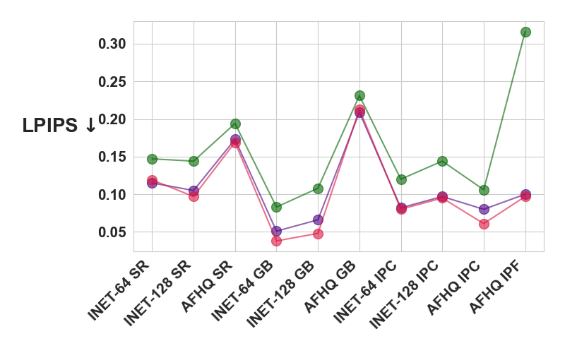
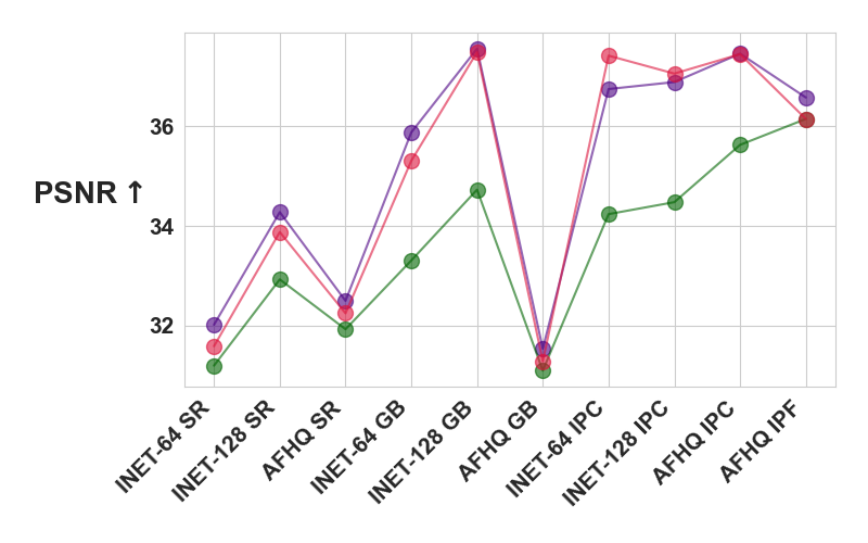
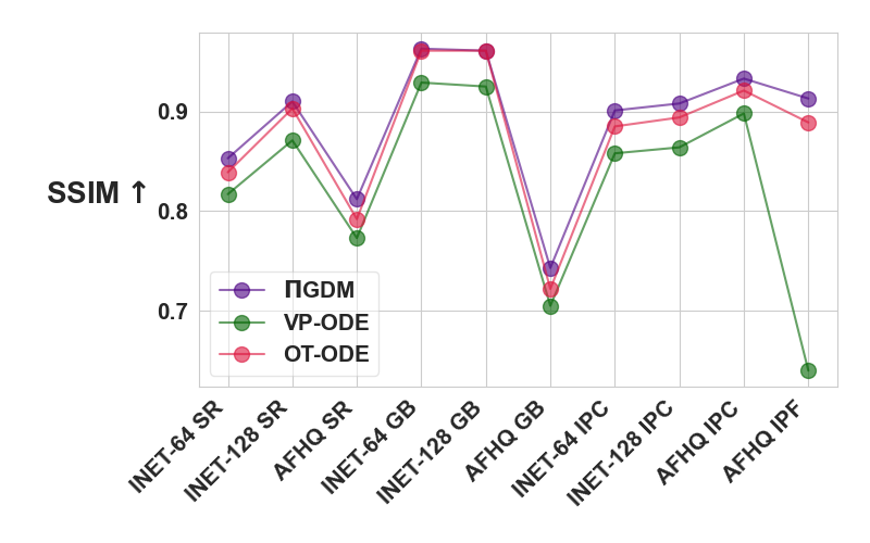
Figure 13: Quantitative evaluation of pretrained conditional OT model for image inversion on super-resolution (SR), gaussian deblurring (GB), image inpainting - centered mask (IPC) and inpainting - freeform (IPF) with $\sigma_{y}=0$. We show results on face-blurred ImageNet-64 (INET-64), face-blurred ImageNet-128 (INET-128), and AFHQ-256 (AFHQ).

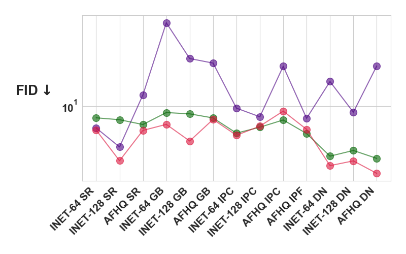
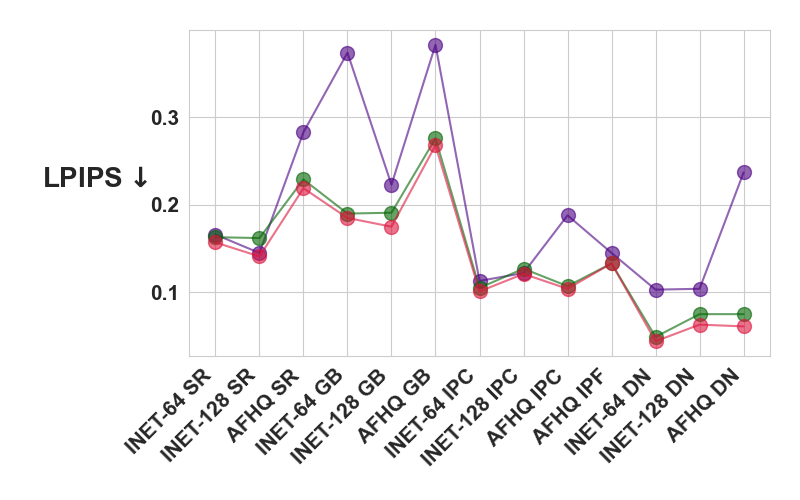
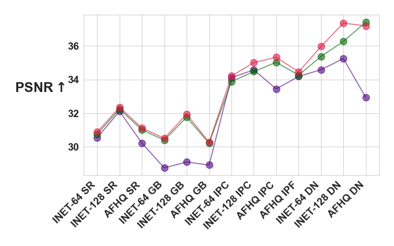
Figure 14: Quantitative evaluation of pretrained conditional OT model for image inversion on super-resolution (SR), gaussian deblurring (GB), image inpainting - centered mask(IPC) and denoising (DN) with $\sigma_{y}=0.05$. We show results on face-blurred ImageNet-64 (INET-64), face-blurred ImageNet-128 (INET-128), and AFHQ-256 (AFHQ).

Table 10: Quantitative evaluation of linear inverse problems on face-blurred ImageNet-$64\times 64$

Model	Inference	NFEs $\downarrow$	SR 2$\times$, $\sigma_{y}=0.05$				Gaussian deblur, $\sigma_{y}=0.05$
			FID $\downarrow$	LPIPS $\downarrow$	PSNR $\uparrow$	SSIM $\uparrow$	FID $\downarrow$	LPIPS $\downarrow$	PSNR $\uparrow$	SSIM $\uparrow$
OT	OT-ODE	80	6.07	0.157	30.88	0.799	6.83	0.185	30.51	0.773
OT	VP-ODE	80	7.82	0.163	30.75	0.792	8.72	0.190	30.40	0.765
OT	$\Pi$GDM	100	6.52	0.168	30.54	0.753	55.19	0.374	28.74	0.516
VP-SDE	OT-ODE	80	5.57	0.155	30.88	0.799	6.33	0.181	30.52	0.773
VP-SDE	VP-ODE	80	7.40	0.160	30.75	0.792	8.16	0.187	30.42	0.766
VP-SDE	$\Pi$GDM	100	6.84	0.174	30.48	0.743	54.77	0.376	28.74	0.511
VP-SDE	RED-Diff	1000	23.02	0.187	31.22	0.839	51.20	0.236	30.19	0.776

Table 11: Quantitative evaluation of linear inverse problems on face-blurred ImageNet-$64\times 64$

Model	Inference	NFEs $\downarrow$	Inpainting-Center, $\sigma_{y}=0.05$				Denoising, $\sigma_{y}=0.05$
			FID $\downarrow$	LPIPS $\downarrow$	SSIM $\uparrow$	PSNR $\uparrow$	FID $\downarrow$	LPIPS $\downarrow$	SSIM $\uparrow$	PSNR $\uparrow$
OT	OT-ODE	80	5.45	0.101	34.21	0.870	2.91	0.044	35.96	0.968
OT	VP-ODE	80	5.70	0.105	33.87	0.865	3.54	0.049	35.37	0.960
OT	$\Pi$GDM	100	9.25	0.111	34.13	0.863	16.59	0.102	34.60	0.906
DDPM	OT-ODE	80	5.03	0.098	34.25	0.872	2.76	0.042	36.02	0.969
VP-SDE	VP-ODE	80	5.26	0.103	33.93	0.866	3.29	0.048	35.45	0.961
VP-SDE	$\Pi$GDM	100	9.75	0.113	34.03	0.860	17.19	0.107	34.25	0.901
VP-SDE	RED-Diff	1000	12.18	0.119	33.97	0.881	6.02	0.041	35.64	0.964

Table 12: Quantitative evaluation of linear inverse problems on face-blurred ImageNet-$64\times 64$

Model	Inference	NFEs $\downarrow$	SR 2$\times$, $\sigma_{y}=0.01$				Gaussian deblur, $\sigma_{y}=0.01$
			FID $\downarrow$	LPIPS $\downarrow$	PSNR $\uparrow$	SSIM $\uparrow$	FID $\downarrow$	LPIPS $\downarrow$	PSNR $\uparrow$	SSIM $\uparrow$
OT	OT-ODE	80	5.39	0.114	31.64	0.838	4.68	0.097	32.09	0.891
OT	VP-ODE	80	5.90	0.120	31.45	0.832	5.58	0.103	31.90	0.884
OT	$\Pi$GDM	100	8.14	0.167	30.01	0.765	26.65	0.223	29.10	0.726
VP-SDE	OT-ODE	80	5.11	0.113	31.64	0.838	4.49	0.094	32.11	0.892
VP-SDE	VP-ODE	80	5.61	0.119	31.46	0.831	5.27	0.101	31.92	0.885
VP-SDE	$\Pi$GDM	100	9.08	0.182	29.82	0.746	26.31	0.238	28.99	0.712
VP-SDE	RED-Diff	1000	12.78	0.131	32.26	0.884	30.65	0.194	31.29	0.832

Table 13: Quantitative evaluation of linear inverse problems on face-blurred ImageNet-$64\times 64$

Model	Inference	NFEs $\downarrow$	Inpainting-Center, $\sigma_{y}=0.01$				Denoising, $\sigma_{y}=0.01$
			FID $\downarrow$	LPIPS $\downarrow$	PSNR $\uparrow$	SSIM $\uparrow$	FID $\downarrow$	LPIPS $\downarrow$	PSNR $\uparrow$	SSIM $\uparrow$
OT	OT-ODE	80	3.86	0.070	37.60	0.894	0.57	0.007	45.21	0.994
OT	VP-ODE	80	4.64	0.085	36.12	0.884	1.96	0.026	39.62	0.981
OT	$\Pi$GDM	100	31.14	0.233	29.73	0.744	61.19	0.298	28.88	0.703
VP-SDE	OT-ODE	80	3.75	0.069	37.77	0.896	0.62	0.006	46.02	0.995
VP-SDE	VP-ODE	80	4.34	0.083	36.19	0.885	1.85	0.025	39.77	0.981
VP-SDE	$\Pi$GDM	100	37.87	0.284	29.32	0.671	69.57	0.382	28.47	0.573
VP-SDE	RED-Diff	1000	7.52	0.083	38.32	0.921	0.63	0.004	45.89	0.995

Table 14: Quantitative evaluation of linear inverse problems on face-blurred ImageNet-$128\times 128$

Model	Inference	NFEs $\downarrow$	SR 2$\times$, $\sigma_{y}=0.05$				Gaussian deblur, $\sigma_{y}=0.05$
			FID $\downarrow$	LPIPS $\downarrow$	PSNR $\uparrow$	SSIM $\uparrow$	FID $\downarrow$	LPIPS $\downarrow$	PSNR $\uparrow$	SSIM $\uparrow$
OT	OT-ODE	70	3.22	0.141	32.35	0.820	4.84	0.175	31.94	0.821
OT	VP-ODE	70	7.52	0.162	32.24	0.847	8.49	0.191	31.76	0.809
OT	$\Pi$GDM	100	4.38	0.148	32.07	0.831	30.30	0.328	29.96	0.606
VP-SDE	OT-ODE	70	3.21	0.139	32.40	0.855	4.49	0.173	32.02	0.824
VP-SDE	VP-ODE	70	9.14	0.166	32.06	0.838	9.35	0.193	31.66	0.804
VP-SDE	$\Pi$GDM	100	7.55	0.183	31.61	0.785	55.61	0.463	28.57	0.414
VP-SDE	RED-Diff	1000	10.54	0.182	31.82	0.852	21.43	0.229	31.41	0.807

Table 15: Quantitative evaluation of linear inverse problems on face-blurred ImageNet-$128\times 128$

Model	Inference	NFEs $\downarrow$	Inpainting-Center, $\sigma_{y}=0.05$				Denoising, $\sigma_{y}=0.05$
			FID $\downarrow$	LPIPS $\downarrow$	PSNR $\uparrow$	SSIM $\uparrow$	FID $\downarrow$	LPIPS $\downarrow$	PSNR $\uparrow$	SSIM $\uparrow$
OT	OT-ODE	70	6.58	0.121	35.00	0.881	3.21	0.063	37.35	0.964
OT	VP-ODE	70	6.44	0.127	34.47	0.871	3.98	0.075	36.26	0.948
OT	$\Pi$GDM	100	7.99	0.122	34.57	0.867	9.60	0.107	35.11	0.903
VP-SDE	OT-ODE	70	6.39	0.120	35.04	0.882	3.25	0.062	37.41	0.965
VP-SDE	VP-ODE	70	8.47	0.129	34.43	0.876	5.83	0.087	35.85	0.938
VP-SDE	$\Pi$GDM	100	9.75	0.130	34.45	0.858	10.69	0.124	34.72	0.882
VP-SDE	RED-Diff	1000	14.63	0.171	32.42	0.820	9.19	0.105	33.52	0.895

Table 16: Quantitative evaluation of linear inverse problems on AFHQ-$256\times 256$

Model	Inference	NFEs $\downarrow$	SR 4$\times$, $\sigma_{y}=0.05$				Gaussian deblur, $\sigma_{y}=0.05$
			FID $\downarrow$	LPIPS $\downarrow$	PSNR $\uparrow$	SSIM $\uparrow$	FID $\downarrow$	LPIPS $\downarrow$	PSNR $\uparrow$	SSIM $\uparrow$
OT	OT-ODE	100	6.03	0.219	31.12	0.739	7.57	0.268	30.27	0.626
OT	VP-ODE	100	6.81	0.229	31.01	0.728	7.80	0.276	30.21	0.616
OT	$\Pi$GDM	100	12.69	0.285	30.18	0.665	24.60	0.383	28.93	0.429
VP-SDE	OT-ODE	100	7.28	0.238	30.83	0.714	8.53	0.276	30.37	0.641
VP-SDE	VP-ODE	100	8.02	0.243	30.96	0.727	10.21	0.289	30.21	0.621
VP-SDE	$\Pi$GDM	100	77.49	0.469	29.34	0.469	116.42	0.535	28.49	0.313
VP-SDE	RED-Diff	1000	20.84	0.331	29.97	0.675	15.81	0.341	30.15	0.645

Table 17: Quantitative evaluation of linear inverse problems on AFHQ-$256\times 256$

Model	Inference	NFEs $\downarrow$	Inpainting-Center, $\sigma_{y}=0.05$				Denoising, $\sigma_{y}=0.05$
			FID $\downarrow$	LPIPS $\downarrow$	PSNR $\uparrow$	SSIM $\uparrow$	FID $\downarrow$	LPIPS $\downarrow$	PSNR $\uparrow$	SSIM $\uparrow$
OT	OT-ODE	100	8.98	0.104	35.32	0.897	2.48	0.061	37.18	0.965
OT	VP-ODE	100	7.48	0.107	35.02	0.892	3.38	0.075	37.41	0.954
OT	$\Pi$GDM	100	19.09	0.153	34.20	0.855	22.87	0.237	32.93	0.823
VP-SDE	OT-ODE	100	9.93	0.107	35.18	0.892	2.17	0.060	37.95	0.963
VP-SDE	VP-ODE	100	8.78	0.107	35.12	0.891	3.08	0.071	37.68	0.959
VP-SDE	$\Pi$GDM	100	57.46	0.239	32.40	0.773	81.15	0.451	29.62	0.639
VP-SDE	RED-Diff	1000	11.02	0.124	34.97	0.893	4.93	0.112	34.18	0.899

Table 18: Quantitative evaluation of linear inverse problems on face-blurred ImageNet-$64\times 64$

Model	Inference	NFEs $\downarrow$	SR 2$\times$, $\sigma_{y}=0$				Gaussian deblur, $\sigma_{y}=0$
			FID $\downarrow$	LPIPS $\downarrow$	PSNR $\uparrow$	SSIM $\uparrow$	FID $\downarrow$	LPIPS $\downarrow$	PSNR $\uparrow$	SSIM $\uparrow$
OT	OT-ODE	80	6.46	0.119	31.59	0.839	2.59	0.038	35.31	0.961
OT	VP-ODE	80	8.29	0.147	31.20	0.817	6.13	0.083	33.31	0.929
OT	$\Pi$GDM	100	6.89	0.115	32.02	0.853	4.53	0.051	35.88	0.963
VP-SDE	OT-ODE	80	6.32	0.118	31.60	0.839	2.61	0.037	35.45	0.963
VP-SDE	VP-ODE	80	7.76	0.145	31.21	0.817	5.68	0.080	33.37	0.931
VP-SDE	$\Pi$GDM	100	6.47	0.113	32.03	0.853	4.35	0.049	35.95	0.964
VP-SDE	RED-Diff	1000	11.74	0.224	30.12	0.798	15.39	0.134	31.99	0.879

Table 19: Quantitative evaluation of linear inverse problems on face-blurred ImageNet-$64\times 64$

Model	Inference	NFEs $\downarrow$	Inpainting-Center, $\sigma_{y}=0$
			FID $\downarrow$	LPIPS $\downarrow$	PSNR $\uparrow$	SSIM $\uparrow$
OT	OT-ODE	80	4.94	0.080	37.42	0.885
OT	VP-ODE	80	7.85	0.120	34.24	0.858
OT	$\Pi$GDM	100	6.09	0.082	36.75	0.901
VP-SDE	OT-ODE	80	4.85	0.079	37.64	0.887
VP-SDE	VP-ODE	80	7.21	0.117	34.33	0.860
VP-SDE	$\Pi$GDM	100	5.79	0.081	36.81	0.902
VP-SDE	RED-Diff	1000	7.29	0.079	39.14	0.925

Table 20: Quantitative evaluation of linear inverse problems on face-blurred ImageNet-$128\times 128$

Model	Inference	NFEs $\downarrow$	Inpainting-Center, $\sigma_{y}=0$
			FID $\downarrow$	LPIPS $\downarrow$	PSNR $\uparrow$	SSIM $\uparrow$
OT	OT-ODE	70	5.88	0.095	37.06	0.894
OT	VP-ODE	70	8.63	0.144	34.48	0.864
OT	$\Pi$GDM	100	5.82	0.097	36.89	0.908
VP-SDE	OT-ODE	70	5.93	0.094	37.31	0.898
VP-SDE	VP-ODE	70	8.08	0.142	34.55	0.865
VP-SDE	$\Pi$GDM	100	5.74	0.095	37.01	0.911
VP-SDE	RED-Diff	1000	5.40	0.068	38.91	0.928

Table 21: Quantitative evaluation of linear inverse problems on face-blurred ImageNet-$128\times 128$

Model	Inference	NFEs $\downarrow$	SR 2$\times$, $\sigma_{y}=0$				Gaussian deblur, $\sigma_{y}=0$
			FID $\downarrow$	LPIPS $\downarrow$	PSNR $\uparrow$	SSIM $\uparrow$	FID $\downarrow$	LPIPS $\downarrow$	PSNR $\uparrow$	SSIM $\uparrow$
OT	OT-ODE	70	4.46	0.097	33.88	0.903	2.09	0.048	37.49	0.961
OT	VP-ODE	70	7.69	0.144	32.93	0.871	6.02	0.108	34.73	0.925
OT	$\Pi$GDM	100	6.09	0.105	34.28	0.910	4.28	0.066	37.56	0.961
VP-SDE	OT-ODE	70	4.62	0.096	33.95	0.906	2.26	0.046	37.79	0.967
VP-SDE	VP-ODE	70	7.91	0.144	32.87	0.869	5.64	0.105	34.81	0.928
VP-SDE	$\Pi$GDM	100	6.02	0.104	34.33	0.911	4.35	0.065	37.70	0.963
VP-SDE	RED-Diff	1000	3.90	0.082	34.47	0.92	4.19	0.085	34.68	0.929

Table 22: Quantitative evaluation of linear inverse problems on AFHQ-$256\times 256$

Model	Inference	NFEs $\downarrow$	SR 4$\times$, $\sigma_{y}=0$				Gaussian deblur, $\sigma_{y}=0$
			FID $\downarrow$	LPIPS $\downarrow$	PSNR $\uparrow$	SSIM $\uparrow$	FID $\downarrow$	LPIPS $\downarrow$	PSNR $\uparrow$	SSIM $\uparrow$
OT	OT-ODE	100	5.75	0.169	32.25	0.792	6.63	0.213	31.29	0.722
OT	VP-ODE	100	6.14	0.194	31.93	0.773	7.38	0.231	31.10	0.705
OT	$\Pi$GDM	100	8.89	0.173	32.57	0.812	9.78	0.209	31.54	0.743
VP-SDE	OT-ODE	100	6.58	0.178	32.18	0.789	8.24	0.226	31.21	0.717
VP-SDE	VP-ODE	100	8.00	0.225	31.48	0.742	9.19	0.252	30.91	0.688
VP-SDE	$\Pi$GDM	100	10.85	0.189	32.52	0.811	11.46	0.228	31.47	0.738
VP-SDE	RED-Diff	1000	8.65	0.191	32.21	0.801	11.67	0.268	31.30	0.731

Table 23: Quantitative evaluation of linear inverse problems on AFHQ-$256\times 256$

Model	Inference	NFEs $\downarrow$	Inpainting-Center, $\sigma_{y}=0$				Inpainting-Free-form, $\sigma_{y}=0$
			FID $\downarrow$	LPIPS $\downarrow$	PSNR $\uparrow$	SSIM $\uparrow$	FID $\downarrow$	LPIPS $\downarrow$	PSNR $\uparrow$	SSIM $\uparrow$
OT	OT-ODE	100	8.87	0.061	37.45	0.921	4.98	0.097	36.15	0.889
OT	VP-ODE	100	9.18	0.106	35.63	0.898	6.92	0.135	34.72	0.869
OT	$\Pi$GDM	100	7.36	0.080	37.45	0.933	6.52	0.100	36.58	0.913
VP-SDE	OT-ODE	100	9.95	0.064	37.49	0.918	5.39	0.099	36.15	0.887
VP-SDE	VP-ODE	100	10.50	0.112	35.59	0.893	7.36	0.139	34.65	0.865
VP-SDE	$\Pi$GDM	100	8.61	0.088	37.27	0.925	7.25	0.109	36.37	0.906
VP-SDE	RED-Diff	1000	8.53	0.050	38.89	0.951	7.27	0.090	36.88	0.892

D.2 Additional qualitative results

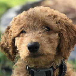
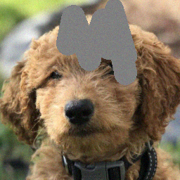
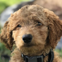
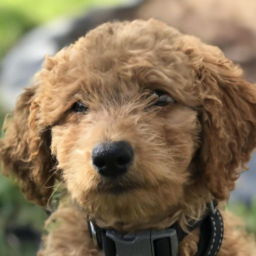
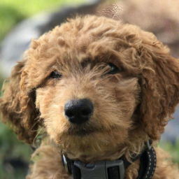
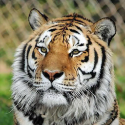
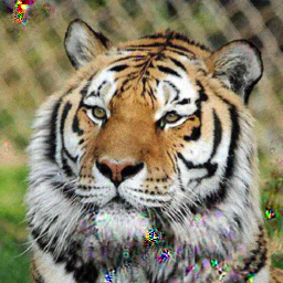
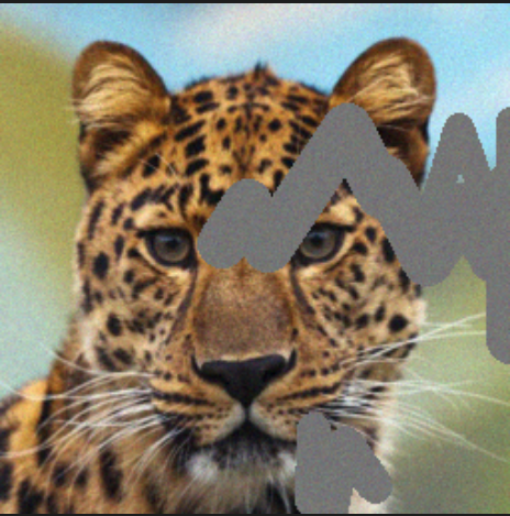
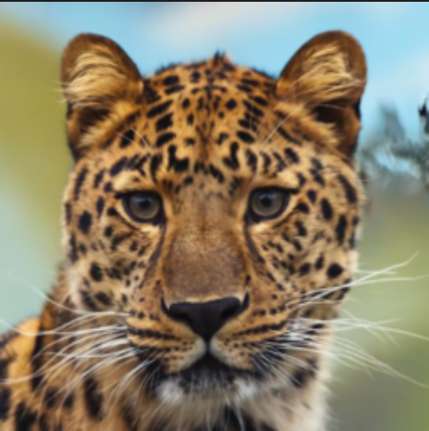
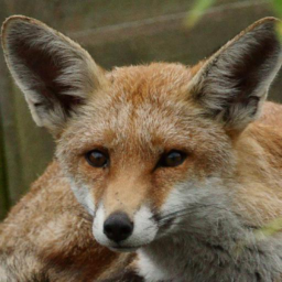
(a) Reference

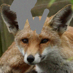
(b) Distorted

(c) OT-ODE

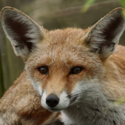
(d) VP-ODE

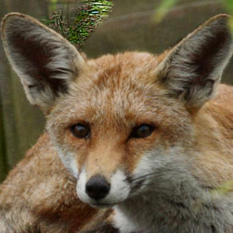
(e) $\Pi$GDM

Figure 18: Image inversion for inpainting (Free-form mask) with conditional OT model and $\sigma_{y}=0.05$ for AFHQ.

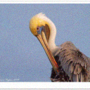
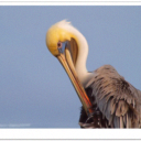
(a) Reference

(b) Distorted

(c) OT-ODE

(d) VP-ODE

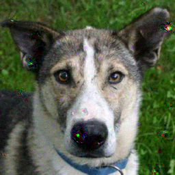
(e) $\Pi$GDM

Figure 19: Image inversion for denoising with conditional OT model and $\sigma_{y}=0.05$ for (first row) ImageNet-64, (second row) ImageNet-128, and (third row) AFHQ.

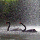
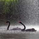
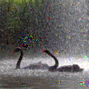
(a) Reference

(b) Distorted

(c) OT-ODE

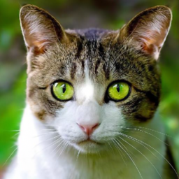
(d) VP-ODE

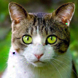
(e) $\Pi$GDM

(f) RED-Diff

Figure 20: Denoising with pretrained VP-SDE model and $\sigma_{y}=0.05$ for (first row) ImageNet-64, (second row) ImageNet-128, and (third row) AFHQ.

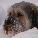
(a) Reference

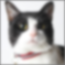
(b) Distorted

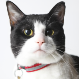
(c) OT-ODE

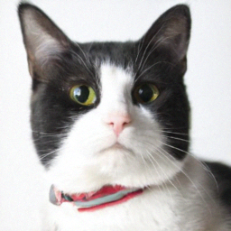
(d) VP-ODE

(e) $\Pi$GDM

Figure 21: Gaussian deblurring with conditional OT model and $\sigma_{y}=0$ for (first row) ImageNet-64, (second row) ImageNet-128 and (third row) AFHQ.

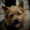
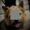
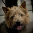
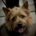
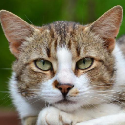
(a) Reference

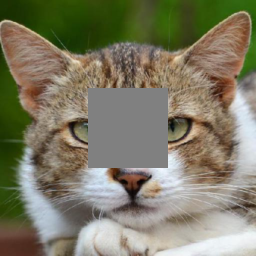
(b) Distorted

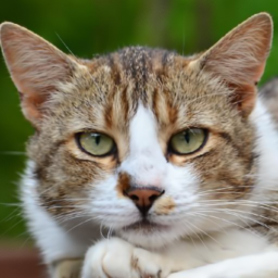
(c) OT-ODE

(d) VP-ODE

(e) $\Pi$GDM

Figure 23: Image inversion for inpainting (centered mask) with conditional OT model and $\sigma_{y}=0$ for (first row) ImageNet-64, (second row) ImageNet-128 and (third row) AFHQ.

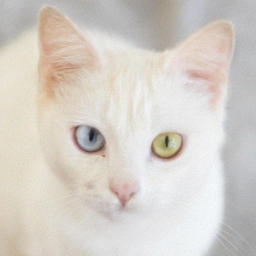
(a) Reference

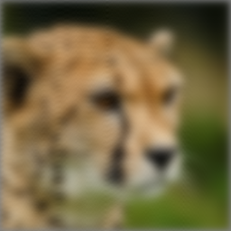
(b) Distorted

(c) OT-ODE

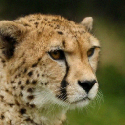
(d) VP-ODE

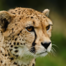
(e) $\Pi$GDM

(f) RED-Diff

Figure 24: Image inversion for Gaussian deblurring with VP-SDE model and $\sigma_{y}=0$ for (first row) ImageNet-64, (second row) ImageNet-128 and (third and fourth row) AFHQ.

(a) Reference

(b) Distorted

(c) OT-ODE

(d) VP-ODE

(e) $\Pi$GDM

(f) RED-Diff

Figure 25: Image inversion for super-resolution with VP-SDE model and $\sigma_{y}=0$ for (first row) ImageNet-64, (second row) ImageNet-128 and (third row) AFHQ.

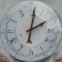
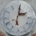
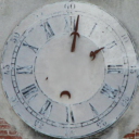
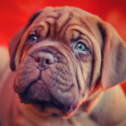
(a) Reference

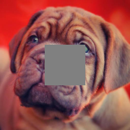
(b) Distorted

(c) OT-ODE

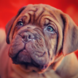
(d) VP-ODE

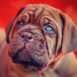
(e) $\Pi$GDM

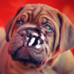
(f) RED-Diff

Figure 26: Image inversion for inpainting (centered mask) with VP-SDE model and $\sigma_{y}=0$ for (first and second row) ImageNet-64, (third row) ImageNet-128 and (fourth row) AFHQ.

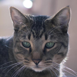
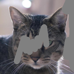
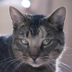
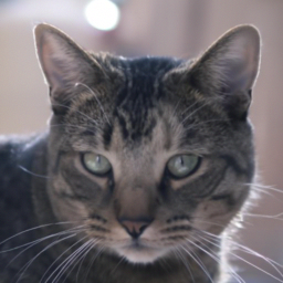
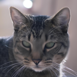
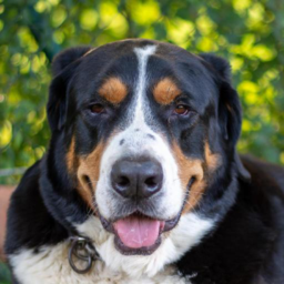
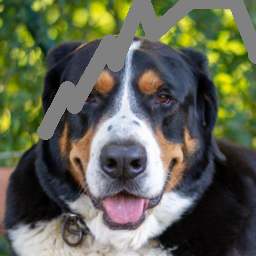
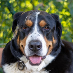
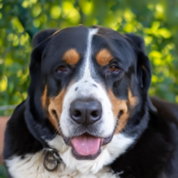
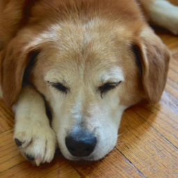
(a) Reference

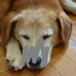
(b) Distorted

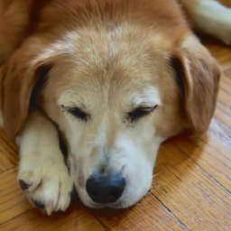
(c) OT-ODE

(d) VP-ODE

(e) $\Pi$GDM

(f) RED-Diff

Figure 27: Image inversion for inpainting (freeform mask) with VP-SDE model and $\sigma_{y}=0$ for AFHQ.

Appendix E Baselines

E.1 $\Pi$GDM

Implementation details.

We closely follow the official code available on github while implementing $\Pi$GDM. For noisy case, we closely follow the Algorithm 1 in the appendix of Song et al. (2022). We use adaptive weighted guidance for both noiseless and noisy cases as in the original work. We always use uniform spacing while iterating the timestep over $100$ steps. We use ascending time from $0$ to $1$. Note that the original paper uses descending time from $T$ to $0$. According to the notational convention used in this paper, this is equivalent to ascending time from $0$ to $1$. For the choice of $r_{t}^{2}$, we consider the values derived from both variance exploding formulation and variance preserving formulation.

Value of $r_{t}^{2}$.

$\Pi$GDM sets the value of $r_{t}^{2}=\frac{\sigma_{1-t}^{2}}{1+\sigma_{1-t}^{2}}$ for VE-SDE, where $q({\bm{x}}_{t}|{\bm{x}}_{1})=\mathcal{N}({\bm{x}}_{1},\sigma_{1-t}^{2}{\bm{I}})$. We can follow the same procedure as outlined in Song et al. (2022), and solve for $r_{t}^{2}$ in closed form for VP-SDE. We know for that VP-SDE, $q({\bm{x}}_{t}|{\bm{x}}_{1})=\mathcal{N}(\alpha_{1-t}{\bm{x}}_{1},(1-\alpha_{1-t}^{2}){\bm{I}})$, where $\alpha_{t}=e^{-\frac{1}{2}T(t)}$, $T(t)=\int_{0}^{t}\beta(s)ds$, and $\beta(s)$ is the noise scale function. Using equation 16 for VP-SDE gives $r_{t}^{2}=1-\alpha_{1-t}^{2}$. We can also obtain an alternate $r_{t}^{2}$ by plugging in value of $\sigma_{t}^{2}$ for VP-SDE into the expression of $r_{t}^{2}$ derived for VE-SDE, which evaluates to $r_{t}^{2}=\frac{1-\alpha_{1-t}^{2}}{2-\alpha_{1-t}^{2}}$. Empirically, we find that $r_{t}^{2}$ for VE-SDE marginally outperforms VP-SDE. We report performance of $\Pi$GDM with both choices of $r_{t}^{2}$ in Table 24, 25 and 26.

Table 24: Relative performance of $\Pi$GDM on ImageNet-$64$ with VE and VP derived $r_{t}^{2}$ with $\sigma_{y}=0.05$

Measurement	Model	VP				VE
		FID $\downarrow$	LPIPS $\downarrow$	PSNR $\uparrow$	SSIM $\uparrow$	FID $\downarrow$	LPIPS $\downarrow$	PSNR $\uparrow$	SSIM $\uparrow$
SR 2$\times$	OT	6.52	0.168	30.54	0.753	5.91	0.160	30.60	0.762
Gaussian deblur	OT	55.19	0.374	28.74	0.516	39.36	0.326	29.00	0.572
Inpainting-Center	OT	9.25	0.111	34.13	0.863	8.70	0.109	34.17	0.864
Denoising	OT	16.59	0.102	34.60	0.906	16.44	0.101	34.64	0.907
SR 2$\times$	VP-SDE	6.84	0.174	30.48	0.743	6.11	0.166	30.54	0.753
Gaussian deblur	VP-SDE	54.77	0.376	28.74	0.511	39.14	0.329	28.99	0.567
Inpainting-Center	VP-SDE	9.75	0.113	34.03	0.860	9.36	0.112	34.06	0.862
Denoising	VP-SDE	17.19	0.107	34.25	0.901	15.54	0.102	34.41	0.906

Table 25: Relative performance of $\Pi$GDM on ImageNet-$128$ with VE and VP derived $r_{t}^{2}$ with $\sigma_{y}=0.05$

Measurement	Model	VP				VE
		FID $\downarrow$	LPIPS $\downarrow$	PSNR $\uparrow$	SSIM $\uparrow$	FID $\downarrow$	LPIPS $\downarrow$	PSNR $\uparrow$	SSIM $\uparrow$
SR 2$\times$	OT	4.38	0.148	32.07	0.831	4.26	0.145	32.12	0.834
Gaussian deblur	OT	30.30	0.328	29.96	0.606	22.42	0.296	30.17	0.642
Inpainting-Center	OT	7.99	0.122	34.57	0.867	7.64	0.120	34.61	0.869
Denoising	OT	9.60	0.107	35.11	0.903	9.30	0.104	35.21	0.906
SR 2$\times$	VP-SDE	7.55	0.183	31.61	0.785	6.14	0.168	31.79	0.803
Gaussian deblur	VP-SDE	55.61	0.463	28.57	0.414	41.69	0.404	28.98	0.493
Inpainting-Center	VP-SDE	9.75	0.130	34.45	0.858	9.46	0.129	34.49	0.859
Denoising	VP-SDE	10.69	0.124	34.72	0.882	10.11	0.119	34.92	0.886

Table 26: Relative performance of $\Pi$GDM on AFHQ with VE and VP derived $r_{t}^{2}$ with $\sigma_{y}=0.05$

Measurement	Model	VP				VE
		FID $\downarrow$	LPIPS $\downarrow$	PSNR $\uparrow$	SSIM $\uparrow$	FID $\downarrow$	LPIPS $\downarrow$	PSNR $\uparrow$	SSIM $\uparrow$
SR $4\times$	OT	12.69	0.285	30.18	0.665	12.31	0.282	30.23	0.672
Gaussian deblur	OT	24.60	0.383	28.93	0.429	19.66	0.355	29.16	0.475
Inpainting-Center	OT	19.09	0.153	34.20	0.855	16.51	0.145	34.40	0.863
Denoising	OT	11.20	0.159	34.49	0.876	10.92	0.153	34.78	0.883
SR $4\times$	VP-SDE	77.49	0.469	29.34	0.469	54.12	0.413	29.73	0.549
Gaussian deblur	VP-SDE	116.42	0.535	28.49	0.313	95.09	0.493	28.74	0.368
Inpainting-Center	VP-SDE	57.46	0.239	32.40	0.773	56.86	0.238	32.42	0.775
Denoising	VP-SDE	81.15	0.451	29.62	0.639	35.33	0.278	31.72	0.776

Choice of starting time.

For OT-ODE sampling and VP-ODE sampling, we observe that starting at time $t>0$ improves the performance. We therefore perform an ablation study on $\Pi$GDM baseline, and vary the start time to verify whether starting at $t>0$ helps to improve the performance. We plot the metrics for three different measurements in  Figure 28. We observe that starting later at time $t>0$ consistently leads to worse performance compared to starting at time $t=0$. Therefore, for all our experiments with $\Pi$GDM, we always start at time $t=0$.

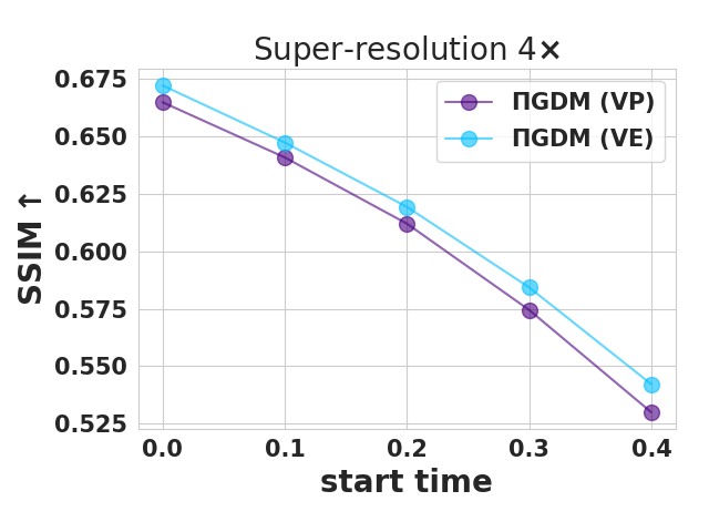
Figure 28: Variation in performance $\Pi$GDM sampling with variation in start times on AFHQ dataset. We use pretrained conditional OT model and set $\sigma_{y}=0.05$. We observe similar trends with VP-SDE checkpoint. We plot metrics for both choices of $r_{t}^{2}$ that can be derived from variance preserving and variance exploding formulations.

E.2 RED-Diff

Implementation details.

We use VP-SDE model for all experiments with RED-Diff. We closely follow the official code available on github while implementing RED-Diff. Similar to (Mardani et al., 2023), we always use uniform spacing while iterating the timestep over $1000$ steps. We use ascending time from $0$ to $1$. Note that the original paper uses descending time from $T$ to $0$. According to the notational convention used in this paper, this is equivalent to ascending time from $0$ to $1$. We use Adam optimizer and use the momentum pair $(0.9,0.99)$ similar to the original work. Further, we use initial learning rate of $0.1$ for AFHQ and ImageNet-128, as used in the original work, and learning rate of $0.01$ for ImageNet-64. We use batch size of $1$ for all the experiments. Finally, we extensively tuned the regularization hyperparameter $\lambda$ to find the value that results in optimal performance across all metrics. We summarize the results of our experiments in Table 27, 28, 29, 30, 31 and 32. We note that more extensive tuning may be able to find better performing hyperparameters but this goes against the intent of a training-free algorithm.

Table 27: Hyperparameter search for RED-Diff on face blurred ImageNet-$64\times 64$ with $\sigma_{y}=0.05$. We use learning rate of $0.01$.

$\lambda$	SR $2\times$, $\sigma_{y}=0.05$				Gaussian deblur, $\sigma_{y}=0.05$
	FID $\downarrow$	LPIPS $\downarrow$	PSNR $\uparrow$	SSIM $\uparrow$	FID $\downarrow$	LPIPS $\downarrow$	PSNR $\uparrow$	SSIM $\uparrow$
0.1	34.09	0.224	30.12	0.798	46.76	0.254	29.29	0.715
0.25	28.45	0.206	30.40	0.814	51.20	0.236	30.19	0.776
0.75	23.02	0.187	31.22	0.839	73.76	0.287	30.47	0.750
1.5	32.35	0.243	30.80	0.792	82.26	0.335	30.29	0.705
2.0	40.33	0.284	30.41	0.750	86.48	0.358	30.17	0.683

$\lambda$	Inpainting-Center, $\sigma_{y}=0.05$				Denoising, $\sigma_{y}=0.05$
	FID $\downarrow$	LPIPS $\downarrow$	PSNR $\uparrow$	SSIM $\uparrow$	FID $\downarrow$	LPIPS $\downarrow$	PSNR $\uparrow$	SSIM $\uparrow$
0.1	15.71	0.155	31.74	0.840	12.47	0.085	32.24	0.907
0.25	15.56	0.155	31.73	0.839	11.80	0.083	32.36	0.908
0.75	13.31	0.139	32.65	0.857	8.43	0.062	33.65	0.932
1.5	12.18	0.119	33.97	0.881	6.11	0.041	35.34	0.958
2.0	12.87	0.119	34.19	0.886	6.02	0.041	35.64	0.964

Table 28: Hyperparameter search for RED-Diff on face blurred ImageNet-$64\times 64$ with $\sigma_{y}=0$. We use learning rate of $0.01$.

$\lambda$	SR $2\times$, $\sigma_{y}=0$				Gaussian deblur, $\sigma_{y}=0$
	FID $\downarrow$	LPIPS $\downarrow$	PSNR $\uparrow$	SSIM $\uparrow$	FID $\downarrow$	LPIPS $\downarrow$	PSNR $\uparrow$	SSIM $\uparrow$
0.1	11.74	0.224	30.12	0.798	15.39	0.134	31.99	0.879
0.25	12.65	0.130	32.34	0.886	29.56	0.236	30.19	0.776
0.75	20.36	0.187	31.22	0.839	55.43	0.287	30.47	0.750
1.5	33.13	0.243	30.80	0.792	71.64	0.335	30.29	0.705
2.0	41.56	0.288	30.46	0.752	78.55	0.358	30.22	0.685

$\lambda$	Inpainting-Center, $\sigma_{y}=0$
	FID $\downarrow$	LPIPS $\downarrow$	PSNR $\uparrow$	SSIM $\uparrow$
0.1	7.29	0.079	39.14	0.925
0.25	7.40	0.155	31.73	0.839
0.75	8.47	0.083	38.59	0.922
1.5	10.75	0.095	37.42	0.916
2.0	12.54	0.119	34.19	0.886

Table 29: Hyperparameter search for RED-Diff on face blurred ImageNet-$128\times 128$ with $\sigma_{y}=0.05$. We use learning rate of $0.1$.

$\lambda$	SR 2$\times$, $\sigma_{y}=0.05$				Gaussian deblur, $\sigma_{y}=0.05$
	FID $\downarrow$	LPIPS $\downarrow$	PSNR $\uparrow$	SSIM $\uparrow$	FID $\downarrow$	LPIPS $\downarrow$	PSNR $\uparrow$	SSIM $\uparrow$
0.1	23.25	0.272	30.12	0.731	37.83	0.42	28.54	0.473
0.75	14.56	0.224	30.71	0.782	21.43	0.229	31.41	0.807
1.5	10.54	0.182	31.82	0.852	22.85	0.247	31.65	0.809
2.0	11.65	0.187	31.93	0.859	24.71	0.259	31.61	0.802

$\lambda$	Inpainting-Center, $\sigma_{y}=0.05$				Denoising, $\sigma_{y}=0.05$
	FID $\downarrow$	LPIPS $\downarrow$	PSNR $\uparrow$	SSIM $\uparrow$	FID $\downarrow$	LPIPS $\downarrow$	PSNR $\uparrow$	SSIM $\uparrow$
0.1	19.68	0.191	31.75	0.795	12.83	0.134	32.27	0.854
0.75	19.03	0.202	31.36	0.779	12.69	0.14	32.09	0.846
1.5	16.33	0.189	31.81	0.794	10.67	0.121	32.89	0.874
2.0	14.63	0.171	32.42	0.819	9.19	0.105	33.52	0.895

Table 30: Hyperparameter search for RED-Diff on face blurred ImageNet-$128\times 128$ with $\sigma_{y}=0$. We use learning rate of $0.1$.

$\lambda$	SR 2$\times$, $\sigma_{y}=0$				Gaussian deblur, $\sigma_{y}=0$
	FID $\downarrow$	LPIPS $\downarrow$	PSNR $\uparrow$	SSIM $\uparrow$	FID $\downarrow$	LPIPS $\downarrow$	PSNR $\uparrow$	SSIM $\uparrow$
0.1	3.90	0.082	34.47	0.922	4.19	0.085	34.68	0.929
0.75	6.52	0.105	33.54	0.905	12.59	0.177	32.71	0.864
1.5	10.46	0.142	32.98	0.894	19.29	0.225	32.15	0.831
2.0	13.08	0.165	32.65	0.884	22.57	0.245	31.94	0.816

$\lambda$	Inpainting-Center, $\sigma_{y}=0$				Inpainting-Freeform, $\sigma_{y}=0$
	FID $\downarrow$	LPIPS $\downarrow$	PSNR $\uparrow$	SSIM $\uparrow$	FID $\downarrow$	LPIPS $\downarrow$	PSNR $\uparrow$	SSIM $\uparrow$
0.1	5.39	0.068	38.91	0.928	8.94	0.162	35.54	0.830
0.75	5.52	0.073	38.11	0.924	9.26	0.166	35.05	0.826
1.5	6.09	0.079	37.32	0.920	10.13	0.172	34.58	0.821
2.0	6.68	0.083	36.87	0.917	10.87	0.176	34.30	0.818

Table 31: Hyperparameter search for RED-Diff on AFHQ with $\sigma_{y}=0.5$. We use learning rate of $0.1$.

$\lambda$	SR $4\times$, $\sigma_{y}=0.05$				Gaussian deblur, $\sigma_{y}=0.05$
	FID $\downarrow$	LPIPS $\downarrow$	PSNR $\uparrow$	SSIM $\uparrow$	FID $\downarrow$	LPIPS $\downarrow$	PSNR $\uparrow$	SSIM $\uparrow$
0.1	21.59	0.385	29.51	0.607	17.36	0.379	29.95	0.639
0.25	22.47	0.374	29.66	0.635	15.81	0.341	30.15	0.645
0.75	20.84	0.331	29.97	0.675	25.41	0.366	29.76	0.588
1.5	22.46	0.355	29.68	0.642	38.66	0.409	29.34	0.525
2.0	25.02	0.376	29.49	0.618	45.01	0.427	29.18	0.500

$\lambda$	Inpainting-Center, $\sigma_{y}=0.05$				Denoising, $\sigma_{y}=0.05$
	FID $\downarrow$	LPIPS $\downarrow$	PSNR $\uparrow$	SSIM $\uparrow$	FID $\downarrow$	LPIPS $\downarrow$	PSNR $\uparrow$	SSIM $\uparrow$
0.1	28.39	0.216	31.53	0.756	8.32	0.159	32.18	0.827
0.25	28.85	0.217	31.51	0.755	8.35	0.161	32.16	0.826
0.75	28.80	0.218	31.64	0.759	7.94	0.156	32.35	0.833
1.5	28.74	0.205	32.19	0.784	6.63	0.138	33.12	0.862
2.0	28.55	0.190	32.63	0.802	5.71	0.124	33.70	0.882
2.5	28.71	0.177	32.99	0.818	4.93	0.111	34.18	0.899

Table 32: Hyperparameter search for RED-Diff on AFHQ with $\sigma_{y}=0$. We use learning rate (lr) of $0.1$ unless mentioned otherwise.

$\lambda$	SR $4\times$, $\sigma_{y}=0$				Gaussian deblur, $\sigma_{y}=0$
	FID $\downarrow$	LPIPS $\downarrow$	PSNR $\uparrow$	SSIM $\uparrow$	FID $\downarrow$	LPIPS $\downarrow$	PSNR $\uparrow$	SSIM $\uparrow$
0.005	11.67	0.197	32.93	0.837	14.69	0.278	31.73	0.760
0.05	8.65	0.191	32.21	0.801	11.67	0.268	31.30	0.731
0.1	9.65	0.204	31.84	0.781	11.53	0.273	31.05	0.711
0.25	11.65	0.222	31.53	0.768	13.22	0.293	30.63	0.675
0.75	14.98	0.274	30.72	0.726	23.34	0.351	29.91	0.598
1.5	19.40	0.332	29.95	0.665	36.96	0.402	29.39	0.529
2.0	22.72	0.361	29.65	0.632	43.64	0.422	29.22	0.504

$\lambda$	Inpainting-Center, $\sigma_{y}=0$, lr=$0.01$				Inpainting-Freeform, $\sigma_{y}=0$
	FID $\downarrow$	LPIPS $\downarrow$	PSNR $\uparrow$	SSIM $\uparrow$	FID $\downarrow$	LPIPS $\downarrow$	PSNR $\uparrow$	SSIM $\uparrow$
0.005	8.53	0.050	38.89	0.951	7.22	0.091	36.89	0.892
0.05	8.53	0.050	38.89	0.951	7.27	0.090	36.88	0.892
0.1	8.53	0.050	38.88	0.951	7.23	0.091	36.82	0.891
0.25	8.53	0.050	38.83	0.950	7.32	0.094	36.69	0.889
0.75	8.88	0.056	38.60	0.948	7.74	0.102	36.26	0.884
1.5	10.32	0.071	38.04	0.942	8.41	0.112	35.69	0.877
2.0	11.62	0.084	37.54	0.937	8.76	0.119	35.37	0.872

References

- Albergo & Vanden-Eijnden (2022) Michael S Albergo and Eric Vanden-Eijnden. Building normalizing flows with stochastic interpolants. arXiv preprint arXiv:2209.15571, 2022.
- Chen (2018) Ricky T. Q. Chen. torchdiffeq, 2018. URL https://github.com/rtqichen/torchdiffeq.
- Chen et al. (2018) Ricky TQ Chen, Yulia Rubanova, Jesse Bettencourt, and David K Duvenaud. Neural ordinary differential equations. Advances in neural information processing systems, 31, 2018.
- Choi et al. (2021) Jooyoung Choi, Sungwon Kim, Yonghyun Jeong, Youngjune Gwon, and Sungroh Yoon. Ilvr: Conditioning method for denoising diffusion probabilistic models. arXiv preprint arXiv:2108.02938, 2021.
- Choi et al. (2020) Yunjey Choi, Youngjung Uh, Jaejun Yoo, and Jung-Woo Ha. Stargan v2: Diverse image synthesis for multiple domains. In Proceedings of the IEEE Conference on Computer Vision and Pattern Recognition, 2020.
- Chung et al. (2022a) Hyungjin Chung, Jeongsol Kim, Michael T Mccann, Marc L Klasky, and Jong Chul Ye. Diffusion posterior sampling for general noisy inverse problems. arXiv preprint arXiv:2209.14687, 2022a.
- Chung et al. (2022b) Hyungjin Chung, Byeongsu Sim, Dohoon Ryu, and Jong Chul Ye. Improving diffusion models for inverse problems using manifold constraints. arXiv preprint arXiv:2206.00941, 2022b.
- Chung et al. (2022c) Hyungjin Chung, Byeongsu Sim, and Jong Chul Ye. Come-closer-diffuse-faster: Accelerating conditional diffusion models for inverse problems through stochastic contraction. In Proceedings of the IEEE/CVF Conference on Computer Vision and Pattern Recognition, pp. 12413–12422, 2022c.
- Chung et al. (2023) Hyungjin Chung, Jeongsol Kim, Sehui Kim, and Jong Chul Ye. Parallel diffusion models of operator and image for blind inverse problems. In Proceedings of the IEEE/CVF Conference on Computer Vision and Pattern Recognition (CVPR), pp. 6059–6069, June 2023.
- Deng et al. (2009) Jia Deng, Wei Dong, Richard Socher, Li-Jia Li, Kai Li, and Li Fei-Fei. Imagenet: A large-scale hierarchical image database. In 2009 IEEE conference on computer vision and pattern recognition, pp. 248–255. Ieee, 2009.
- Detlefsen et al. (2022) Nicki Skafte Detlefsen, Jiri Borovec, Justus Schock, Ananya Harsh Jha, Teddy Koker, Luca Di Liello, Daniel Stancl, Changsheng Quan, Maxim Grechkin, and William Falcon. Torchmetrics-measuring reproducibility in pytorch. Journal of Open Source Software, 7(70):4101, 2022.
- Elad et al. (2023) Michael Elad, Bahjat Kawar, and Gregory Vaksman. Image denoising: The deep learning revolution and beyond—a survey paper. SIAM Journal on Imaging Sciences, 16(3):1594–1654, 2023.
- Heusel et al. (2017) Martin Heusel, Hubert Ramsauer, Thomas Unterthiner, Bernhard Nessler, and Sepp Hochreiter. Gans trained by a two time-scale update rule converge to a local nash equilibrium. Advances in neural information processing systems, 30, 2017.
- Ho et al. (2020) Jonathan Ho, Ajay Jain, and Pieter Abbeel. Denoising diffusion probabilistic models. Neural Information Processing Systems (NeurIPS), 2020.
- Jalal et al. (2021) Ajil Jalal, Marius Arvinte, Giannis Daras, Eric Price, Alexandros G Dimakis, and Jon Tamir. Robust compressed sensing mri with deep generative priors. Advances in Neural Information Processing Systems, 34:14938–14954, 2021.
- Kadkhodaie & Simoncelli (2020) Zahra Kadkhodaie and Eero P Simoncelli. Solving linear inverse problems using the prior implicit in a denoiser. arXiv preprint arXiv:2007.13640, 2020.
- Karras et al. (2022) Tero Karras, Miika Aittala, Timo Aila, and Samuli Laine. Elucidating the design space of diffusion-based generative models. Advances in Neural Information Processing Systems, 35:26565–26577, 2022.
- Kawar et al. (2021) Bahjat Kawar, Gregory Vaksman, and Michael Elad. Snips: Solving noisy inverse problems stochastically. Advances in Neural Information Processing Systems, 34:21757–21769, 2021.
- Kawar et al. (2022) Bahjat Kawar, Michael Elad, Stefano Ermon, and Jiaming Song. Denoising diffusion restoration models. Advances in Neural Information Processing Systems, 35:23593–23606, 2022.
- Kingma et al. (2021) Diederik Kingma, Tim Salimans, Ben Poole, and Jonathan Ho. Variational diffusion models. Advances in neural information processing systems, 34:21696–21707, 2021.
- Kingma & Gao (2023) Diederik P. Kingma and Ruiqi Gao. Vdm++: Variational diffusion models for high-quality synthesis, 2023.
- Lin et al. (2023) Shanchuan Lin, Bingchen Liu, Jiashi Li, and Xiao Yang. Common diffusion noise schedules and sample steps are flawed. arXiv preprint arXiv:2305.08891, 2023.
- Lipman et al. (2022) Yaron Lipman, Ricky TQ Chen, Heli Ben-Hamu, Maximilian Nickel, and Matt Le. Flow matching for generative modeling. arXiv preprint arXiv:2210.02747, 2022.
- Liu et al. (2022) Xingchao Liu, Chengyue Gong, and Qiang Liu. Flow straight and fast: Learning to generate and transfer data with rectified flow. arXiv preprint arXiv:2209.03003, 2022.
- Mardani et al. (2023) Morteza Mardani, Jiaming Song, Jan Kautz, and Arash Vahdat. A variational perspective on solving inverse problems with diffusion models. arXiv preprint arXiv:2305.04391, 2023.
- McCann (1997) Robert J McCann. A convexity principle for interacting gases. Advances in mathematics, 128(1):153–179, 1997.
- Murata et al. (2023) Naoki Murata, Koichi Saito, Chieh-Hsin Lai, Yuhta Takida, Toshimitsu Uesaka, Yuki Mitsufuji, and Stefano Ermon. Gibbsddrm: A partially collapsed gibbs sampler for solving blind inverse problems with denoising diffusion restoration, 2023.
- Robbins (1992) Herbert E Robbins. An empirical bayes approach to statistics. In Breakthroughs in Statistics: Foundations and basic theory, pp. 388–394. Springer, 1992.
- Rout et al. (2023) Litu Rout, Negin Raoof, Giannis Daras, Constantine Caramanis, Alexandros G Dimakis, and Sanjay Shakkottai. Solving linear inverse problems provably via posterior sampling with latent diffusion models. arXiv preprint arXiv:2307.00619, 2023.
- Saharia et al. (2022a) Chitwan Saharia, William Chan, Huiwen Chang, Chris Lee, Jonathan Ho, Tim Salimans, David Fleet, and Mohammad Norouzi. Palette: Image-to-image diffusion models. In ACM SIGGRAPH 2022 Conference Proceedings, pp. 1–10, 2022a.
- Saharia et al. (2022b) Chitwan Saharia, Jonathan Ho, William Chan, Tim Salimans, David J Fleet, and Mohammad Norouzi. Image super-resolution via iterative refinement. IEEE Transactions on Pattern Analysis and Machine Intelligence, 45(4):4713–4726, 2022b.
- Shaul et al. (2023) Neta Shaul, Ricky TQ Chen, Maximilian Nickel, Matthew Le, and Yaron Lipman. On kinetic optimal probability paths for generative models. In International Conference on Machine Learning, pp. 30883–30907. PMLR, 2023.
- Sohl-Dickstein et al. (2015) Jascha Sohl-Dickstein, Eric Weiss, Niru Maheswaranathan, and Surya Ganguli. Deep unsupervised learning using nonequilibrium thermodynamics. In International Conference on Machine Learning (ICML), 2015.
- Song et al. (2021a) Jiaming Song, Chenlin Meng, and Stefano Ermon. Denoising diffusion implicit models. In International Conference on Learning Representations (ICLR), 2021a.
- Song et al. (2022) Jiaming Song, Arash Vahdat, Morteza Mardani, and Jan Kautz. Pseudoinverse-guided diffusion models for inverse problems. In International Conference on Learning Representations, 2022.
- Song & Ermon (2019) Yang Song and Stefano Ermon. Generative modeling by estimating gradients of the data distribution. Neural Information Processing Systems (NeurIPS), 2019.
- Song et al. (2021b) Yang Song, Conor Durkan, Iain Murray, and Stefano Ermon. Maximum likelihood training of score-based diffusion models. Advances in Neural Information Processing Systems, 34:1415–1428, 2021b.
- Song et al. (2021c) Yang Song, Jascha Sohl-Dickstein, Diederik P Kingma, Abhishek Kumar, Stefano Ermon, and Ben Poole. Score-based generative modeling through stochastic differential equations. In International Conference on Learning Representations (ICLR), 2021c.
- Wang et al. (2022) Yinhuai Wang, Jiwen Yu, and Jian Zhang. Zero-shot image restoration using denoising diffusion null-space model. arXiv preprint arXiv:2212.00490, 2022.
- Yang et al. (2022) Kaiyu Yang, Jacqueline H Yau, Li Fei-Fei, Jia Deng, and Olga Russakovsky. A study of face obfuscation in imagenet. In International Conference on Machine Learning, pp. 25313–25330. PMLR, 2022.
- Zhang et al. (2018) Richard Zhang, Phillip Isola, Alexei A Efros, Eli Shechtman, and Oliver Wang. The unreasonable effectiveness of deep features as a perceptual metric. In CVPR, 2018.