Joint inversion of Time-Lapse Surface Gravity and Seismic Data for Monitoring of 3D CO₂ Plumes via Deep Learning

Abstract.

We introduce a fully 3D, deep learning-based approach for the joint inversion of time-lapse surface gravity and seismic data for reconstructing subsurface density and velocity models. The target application of this proposed inversion approach is the prediction of subsurface CO₂ plumes as a complementary tool for monitoring CO₂ sequestration deployments. Our joint inversion technique outperforms deep learning-based gravity-only and seismic-only inversion models, achieving improved density and velocity reconstruction, accurate segmentation, and higher R-squared coefficients. These results indicate that deep learning-based joint inversion is an effective tool for CO₂ storage monitoring. Future work will focus on validating our approach with larger datasets, simulations with other geological storage sites, and ultimately field data.

1. Introduction

Reducing CO₂ concentration in the atmosphere is critical to control climate change. These efforts involve implementing various technologies, such as efficient fossil-based fuel consumption, expanding absorption sources through afforestation/reforestation, and adopting CO₂ capture, utilization, and storage (CCUS) techniques.

Among the CCUS technologies currently deployed worldwide, CO₂ geological storage has emerged as a promising approach. This technology involves capturing CO₂ from fixed sources or directly from air, then injecting it into underground formations.

Injecting CO₂ is just part of the process; during and after injection, ensuring the integrity of these geological sites necessitates ongoing monitoring. Regulatory authorities mandate the demonstration of storage volume containment and the detection of any potential CO₂ leakage or unwanted migration. Given the time scales involved in monitoring CO₂ storage sites, traditional monitoring techniques based on borehole sensors or surface seismic monitoring may not be practical or economically viable. Remote sensing by other modes, such as gravity, might be economically viable and technically feasible if combined with traditional seismic approaches.

Once data from the field is recorded, geophysical inversion techniques are deployed. These widely used techniques for interpreting data sets and recovering subsurface physical models can be crucial in monitoring CO₂ storage sites (Fawad and Mondol, 2021; Alyousuf et al., 2022). The recovered models, which encompass parameters such as velocity, density, resistivity, or saturation, provide essential information about the structural and compositional characteristics of the subsurface.

Integrating multiple datasets collected over the same area is known as geophysical inversion (Hu et al., 2023; Sun et al., 2020). This approach enhances the reconstruction of subsurface structures and facilitates the identification of changes or anomalies associated with activities like CO₂ storage (Um et al., 2022). However, effectively integrating the information embedded in multiple geophysical datasets presents a practical challenge from a computational point of view (i.e., storage, memory, and compute time), which compounds the inherent difficulties of solving nonlinear inversion problems (Tarantola and Valette, 1981). These challenges especially become apparent when working with realistic 3D synthetic or field data.

In this work, we develop an effective supervised 3D deep learning (DL)-based inversion method to recover high-resolution subsurface CO₂ plumes from both surface gravity and seismic data. To the best of our knowledge, this is the first fully 3D approach for the joint inversion of surface gravity and seismic data, which is tested on realistic, physics-simulated CO₂ plumes.

2. Previous Work

Conventional inversion methods find a model with the minimum possible structure and whose forward response fits the observed data (De Groot-Hedlin and Constable, 1990; Li and Oldenburg, 1998; Nabighian et al., 2005). The minimum structure is achieved by minimizing model roughness through a least squares regression, resulting in a smooth model. While the least squares regression produces smooth subsurface models, the predicted models are often larger and exhibit smaller density values than the actual model (Boulanger and Chouteau, 2001; Rezaie et al., 2017).

DL is an emerging alternative to traditional geophysical inversion (Jin et al., 2017; Araya-Polo et al., 2018; Kim and Nakata, 2018; Yang and Ma, 2019). Over the last several years, deep convolutional neural networks (CNNs) have achieved state-of-the-art results in various computer vision applications such as image classification, segmentation, and generation (Deng et al., 2009; Bakas et al., 2018; Karras et al., 2019). CNNs have recently been used for inversion of seismic (Adler et al., 2021; Chen et al., 2020; Li et al., 2020), electromagnetic imaging (Colombo et al., 2020; Oh et al., 2020), electrical resistivity (Liu et al., 2020; Shahriari et al., 2020), and time-lapse surface gravity data (Yang et al., 2022; Yu-Feng et al., 2021; Huang et al., 2021; Celaya et al., 2023b). However, these works focus solely on inverting a single modality and do not explore joint inversion with multiphysical data.

Using simulated CO₂ plumes from the onshore Kimberlina site, Um et al. developed a 2D DL architecture to perform a joint inversion with seismic, electromagnetic, and gravity data (Um et al., 2022). Additionally, they use a modified version of their architecture to invert their imaging data types individually. In each case, their DL-based approach can recover CO₂ plumes. However, their approach still does not perform DL-based inversion in a fully 3D setting. Hu et al. present a physics-informed DL-based approach for inverting electromagnetic and seismic data for recovering subsurface anomalies (Hu et al., 2023). While their approach successfully reconstructs the anomalies, this approach also uses 2D data and does not consider 3D data or the computational cost of implementing physics-informed inversion for such data; as opposed to our work, which implements fully 3D joint inversion with seismic and surface gravity data.

3. Problem Statement

Classical inversion techniques aim to minimize a cost function that measures the difference between the forward response of a given subsurface model and the observed data. Let $F$ be our forward operator, $\mathbf{m}$ be a subsurface model, and $\mathbf{d}_{\text{obs}}$ be the observed data. Then the classical inversion problem can be written as

(1) $$\min_{\mathbf{m}}||F(\mathbf{m})-\mathbf{d}_{\text{obs}}||_{2}^{2}.$$

Note that this problem takes a single input (i.e., $\mathbf{d}_{\text{obs}}$) and produces a single predicted subsurface model.

In contrast, joint inversion is an extension of the classical formulation given by (1) that maps multiple inputs (i.e., gravity, seismic, and electromagnetic data) to multiple outputs (i.e., density, velocity, and resistivity models). For a given number of inputs $\mathbf{d}_{\text{obs}}^{1},\dots,\mathbf{d}_{\text{obs}}^{n}$ and appropriate forward operators $F_{1},\dots,F_{n}$, our joint problem is given by

(2) $$\min_{\mathbf{m}^{1},\dots\mathbf{m}^{n}}\sum_{i=1}^{n}||F_{i}(\mathbf{m}^{i})-\mathbf{d}_{\text{obs}}^{i}||_{2}^{2}+\alpha\sum_{i\neq j}\Phi(\mathbf{m}^{i},\mathbf{m}^{j}),$$

where $\Phi$ is a coupling function used to link different physical models via known petrophysical relations or other metrics like SSIM, and $\alpha$ is a parameter controlling the contribution of the coupling term (Moorkamp et al., 2011; Lelièvre et al., 2012). Joint inversion is much more time-consuming than independent inversions because of the additional terms in the cost function and the need to exchange information between different models via the coupling terms (Hu et al., 2023). There also is a need to determine or adjust the weighting parameter $\alpha$, which adds another layer of complexity to the standard joint inversion method (Hu et al., 2023).

Our goal is to train a CNN that can accurately predict the changes in subsurface density and velocity given corresponding variations in surface gravity and seismic data.

4. Data Preparation

Located 60km off the western coast of Norway, the Johansen formation is a promising CO₂ storage site with a theoretical capacity exceeding 1Gt of CO₂. The formation encompasses an aquifer with an approximate thickness of 100m, spans 100km in the north-south direction and 60km from east to west, and is at a depth that ranges from 2,200m to 3,100m below sea level. This setting provides optimal pressure and temperature conditions for injecting CO₂ in a supercritical state.

We generate data based on the Johansen formation using the process described in (Celaya et al., 2023b). That is, we generate a number of distinct geological realizations that vary in porosity and permeability. We conduct a fluid flow simulation that assumes a 100-year injection period followed by a 400-year migration period. This process produces subsurface changes in density. To convert these density models to $V_{p}$ models for forward seismic modeling, we use the following conversion:

(3) $$V_{p}(\mathbf{r})=\sqrt{\frac{\kappa+\frac{4}{3}\mu}{\rho(\mathbf{r})}},$$

where $\mathbf{r}$ is the spatial coordinate in our model, $\kappa=8.14$GPa is the bulk modulus, $\mu=1.36$GPa is the shear modulus, and $\rho$ is the density value (Hoek and Bray, 1981; Pariseau, 2017). Here, we assume that the formation comprises 80% shale and 20% sandstone to get the values for $\kappa$ and $\mu$ (Sundal et al., 2016; Eigestad et al., 2009). Using this process, we generate 180 density/velocity pairs. For preprocessing, we resample each density and velocity model from their original resolution of 440$\times$530$\times$145 to 256$\times$256$\times$128.

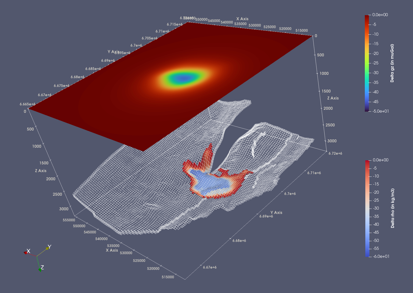
Figure 1. Illustration of a change in surface gravity for a given density perturbation in the subsurface (Celaya et al., 2023b).

4.1. Modeling Gravity

Given a density perturbation $\Delta\rho$ observed between the current and original (i.e., base) acquisition, the gravity field recorded at a station located at $\mathbf{r^{\prime}}$ can be expressed as:

(4) $$\mathbf{g}(\mathbf{r^{\prime}})=\gamma\iiint_{V}\frac{\mathbf{r}-\mathbf{r^{\prime}}}{||\mathbf{r}-\mathbf{r^{\prime}}||_{2}^{3}}\Delta\rho(\mathbf{r})dV$$

where $V$ is the volume of the reservoir, and $\gamma$ is Newton’s gravitational constant. For more details on gravity modeling, see (Celaya et al., 2023b). Assuming that gravity sensors are placed in a uniform grid every 500m, our surface gravity maps are size 88$\times$106. An illustration of a change in surface gravity for a given density permutation in the subsurface is shown in Figure 1.

4.2. Forward Seismic Modeling

Forward seismic modeling approximates the behavior of seismic waves propagating through a mechanical medium $\mathbf{m}$ and is given by the elastic wave equation:

(5) $$\frac{\partial^{2}u}{\partial t^{2}}-\mathbf{V}_{p}^{2}\nabla(\nabla\cdot u)-\mathbf{V}_{s}^{2}\Delta u=\mathbf{f},$$

where $\mathbf{u}=\mathbf{u}(x,y,z,t)$, is the seismic wave displacement, $\mathbf{V}_{p}$ is P-wave velocity (compression/rarefaction), $\mathbf{V}_{s}$ is S-wave velocity (shear stress), and $\mathbf{f}$ is the perturbation source (i.e., shot) function (Gelboim et al., 2022). While (5) more accurately describes seismic wave propagation, it is often preferred (as in this work) to approximate the solution $\mathbf{u}$ by the acoustic wave equation, which assumes only P-waves and requires less computational resources and parameters, as compared to solving (5) (Gelboim et al., 2022).

3D seismic data consumes a large amount of memory and storage, up to dozens of TB for the raw data in our case. We compute spatial decimation evenly, but temporal, which in seismic signals represents depth, decimation favors samples that convey information in the area of interest (i.e., the reservoir). Further, we collapse our seismic data by adding the recorded data from each shot and then boost the later time signals by multiplying by a monotonically increasing function. This method is fully described in (Gelboim et al., 2022). Finally, we resize each collapsed and boosted seismic cube from its original resolution of 167$\times$154$\times$941 to 256$\times$256$\times$512 by first taking every other slice (i.e., time step) in the z-direction and then linearly interpolating to the final resolution.

Like forward gravity modeling, we look at the differences between the original or base seismic data and the current data. Figure 2 illustrates an example of the change in seismic data from the original and current acquisitions.

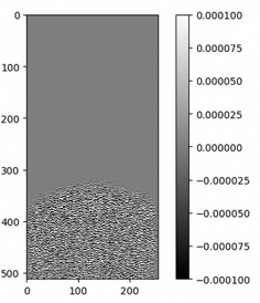
Figure 2. Example of seismic difference cube.

5. Methods

5.1. Network Architecture

We use a modified 3D U-Net architecture to map 2D surface gravity maps and 3D seismic cubes to subsurface changes in density and velocity. Each input is fed into a dedicated encoder branch. The first step for the surface gravity encoder branch is to resize the input to match the reservoir geometry via linear interpolation. Then the 2D features are converted into a 3D volume using a pointwise convolution, where the number of channels equals the subsurface model’s depth (i.e., the output). This resulting 3D volume is the input to the first 3D encoder branch of the network. The seismic encoder branch starts with a 3D seismic cube as input. However, the seismic cubes are larger in the depth dimension than the network output. To address this, we use two convolutional layers with strides 1$\times$1$\times$2 to reduce the depth dimension of the seismic cube from 512 to 128. The resulting resized seismic features are the input to the second encoder branch of our architecture. In each resolution level of our encoder branch, we apply two convolutional layers and downsampling via max pooling four times. A convolutional layer consists of two convolutions, each followed by batch normalization and a ReLU non-linearity.

At the bottleneck of our architecture, we concatenate the encoded seismic and gravity features and apply two convolutional layers to merge the individual features. We also apply autoencoder regularization. However, because we have two inputs, we separately decode the seismic and gravity features (before concatenation and convolution) to reconstruct their respective inputs.

Our decoder branch upsamples the combined features and concatenates them with the corresponding features from the encoder branches in the skip connections. Like with the network proposed by (Celaya et al., 2023b), we split the output of the decoder branch into three separate outputs: two regression branches to predict density and velocity and one for segmenting the plume. Figure 3 shows a detailed sketch of our proposed architecture.

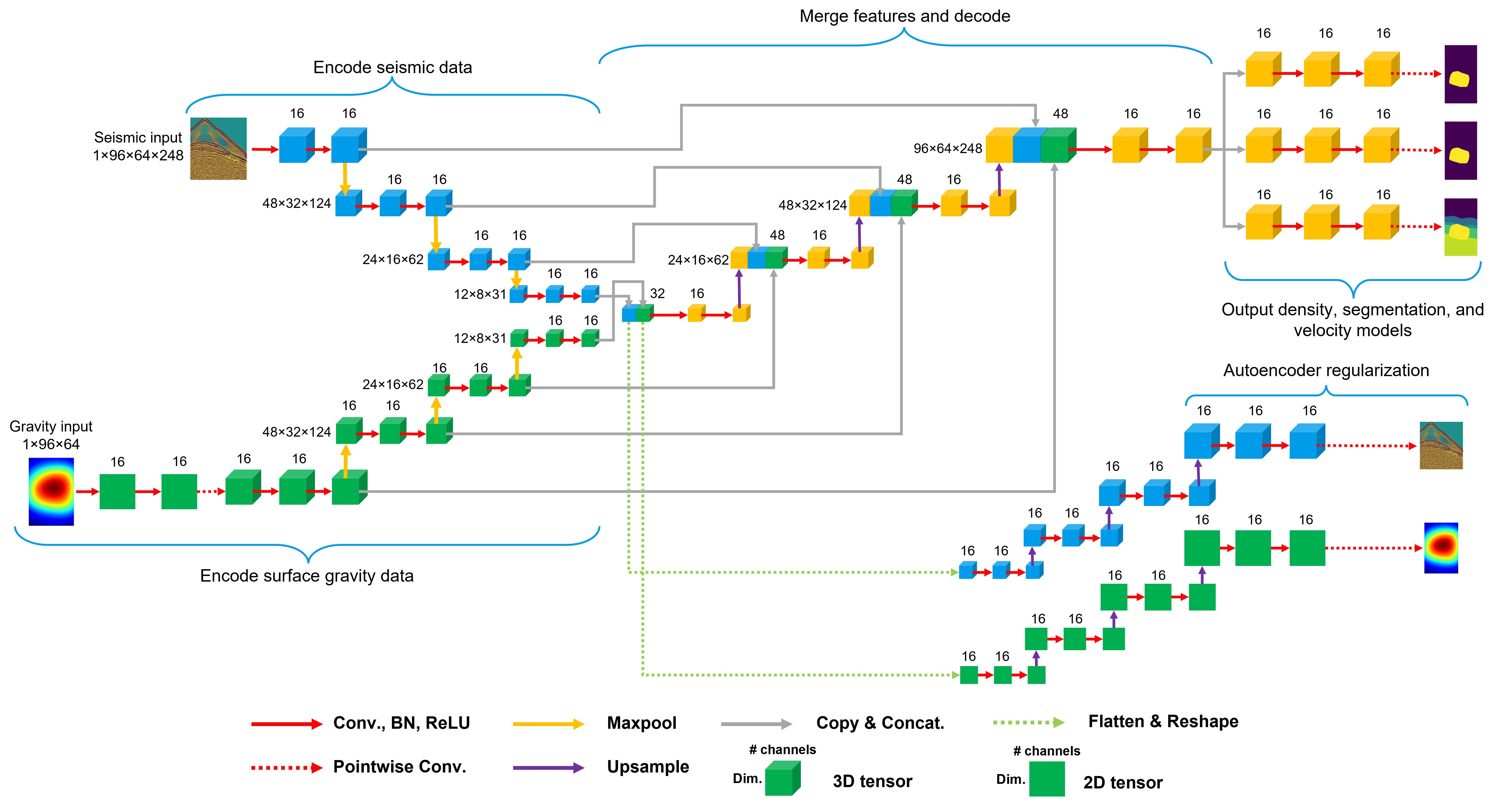
Figure 3. Detailed sketch of our proposed architecture for jointly inverting surface gravity and seismic data. Our architecture uses two separate encoder branches for each input and decodes them jointly. The output of the decoder branch splits into three separate outputs: two regression branches to predict density and velocity and one for segmenting the plume. Additionally, this architecture uses autoencoder regularization.

5.2. Loss Function

Our loss function consists of three components - segmentation, regression, autoencoder losses.

The segmentation loss is the Generalized Dice Loss (GDL) proposed by Sudre et al. (Sudre et al., 2017). Unlike the original Dice loss proposed by (Milletari et al., 2016), the GDL uses weighting terms to account for class imbalance. This loss function is given by

(6) $$\mathcal{L}_{gdl}=\frac{\sum_{k=1}^{C}w_{k}||T^{k}-P^{k}||_{2}^{2}}{\sum_{k=1}^{C}w_{k}\left(||T^{k}||_{2}^{2}+||P^{k}||_{2}^{2}\right)},$$

where $C$ denotes the number of segmentation classes, $P^{k}$ is the $k$-th class in the predicted mask, and $T^{k}$ is the same for the ground truth. The term $w_{k}$ is the weighting term for the $k^{th}$ class and is given by $w_{k}=\left(\frac{1}{\sum_{j=1}^{C}\frac{1}{N_{j}}}\right)\frac{1}{N_{k}}$. Here, $N_{k}$ is the total number of pixels belonging to the class $k$ over the entire dataset. Note that the weights $w_{k}$ are pre-computed and remain constant throughout training. In our case, the number of segmentation classes equals two; background and foreground. The computed class weights are approximately 0.0015 and 0.9985 for the background and foreground classes, respectively.

The regression and autoencoder losses use the mean squared error loss for their respective inputs. For a general input pair $(T,P)$, this loss is given by $\frac{1}{N}||T-P||_{2}^{2}$. For the regression tasks (i.e., density and velocity reconstruction) the inputs to this loss function are the true and predicted density and velocity models. For the autoencoder branches, the inputs to this loss function are the true and reconstructed gravity and seismic inputs.

Our overall loss function is a weighted convex combination of the previously described components and is given by

(7) $$\mathcal{L}=0.375\mathcal{L}_{\rho}+0.2\mathcal{L}_{gdl}+0.375\mathcal{L}_{v}+\frac{0.05}{2}\left(\mathcal{L}_{ae}^{grav}+\mathcal{L}_{ae}^{seis}\right),$$

where $\mathcal{L}_{\rho}$, $\mathcal{L}_{gdl}$, $\mathcal{L}_{v}$, $\mathcal{L}_{ae}^{grav}$, and $\mathcal{L}_{ae}^{seis}$ are the density model, segmentation, velocity model, gravity autoencoder, and seismic autoencoder losses, respectively. Note that we select these weights via a partial grid search.

5.3. Training and Testing Protocols

To train our neural networks, we use the Adam optimizer (Kingma and Ba, 2014) with an initial learning rate of 0.001 and a cosine decay schedule with restarts (Loshchilov and Hutter, 2017). We train our model to convergence ($\approx 400$ epochs) with a batch size of 8. We use 80% of our dataset as a training set, use 10% of the training data as a validation set, and use the remaining 20% of the data as a test set. To compare the effect of joint inversion vs. inversion with only gravity or seismic data, we use the architecture described in (Celaya et al., 2023b) for the portions of our dataset corresponding to either gravity or seismic inversion. Note that the models used for individual inversion only output the properties corresponding to that particular inversion problem. For example, the network used for purely seismic inversion only produces a velocity model as a prediction.

To evaluate the validity of our predicted inversions, we utilize the following metrics: mean squared error in kg/m³ between the true and predicted density models, mean squared error in m/s between the true and predicted velocity models, mean squared error in $\mu$Gals between the observed data and the gravity response of the predicted density model, the R-squared coefficient between the true and predicted models (for density and velocity), and the Dice coefficient between the non-zero masks of the true and predicted plume geometry.

Our models are implemented in Python using PyTorch (v2.0.1) and trained on four NVIDIA A100 GPUs (Paszke et al., 2019). At test time, our DL-based methods produce predictions of size 256$\times$256$\times$128. We resample this output to the original grid resolution of 440$\times$530$\times$145 via linear interpolation to produce our final prediction. Given the sample size, we develop a data parallelism approach by using PyTorch’s Distributed Data Parallel implementation. The in-node scalability is nearly ideal, with epochs taking 190 seconds running on 1 GPU and ending up in 45 seconds when running on 4 GPUs.

Method	MSE (kg/m3)	MSE (m/s)	MSE ($\mu$Gal)	Dice	R-Squared
					Density	Velocity
Gravity	0.311 (0.215)	-	0.601 (1.185)	0.589 (0.034)	0.769 (0.12)	-
Seismic	-	0.121 (0.100)	-	0.579 (0.096)	-	0.715 (0.175)
Joint	0.268 (0.174)	0.084 (0.057)	0.634 (1.241)	0.621 (0.038)	0.801 (0.095)	0.800 (0.095)

Table 1. Joint inversion vs. inversion with only gravity or seismic data. Here, we see that our proposed joint inversion generally outperforms gravity and seismic-only inversion for all metrics except for the mean squared error between the observed data and the gravity response of the predicted density model, where the results vs. the gravity-only model are comparable.

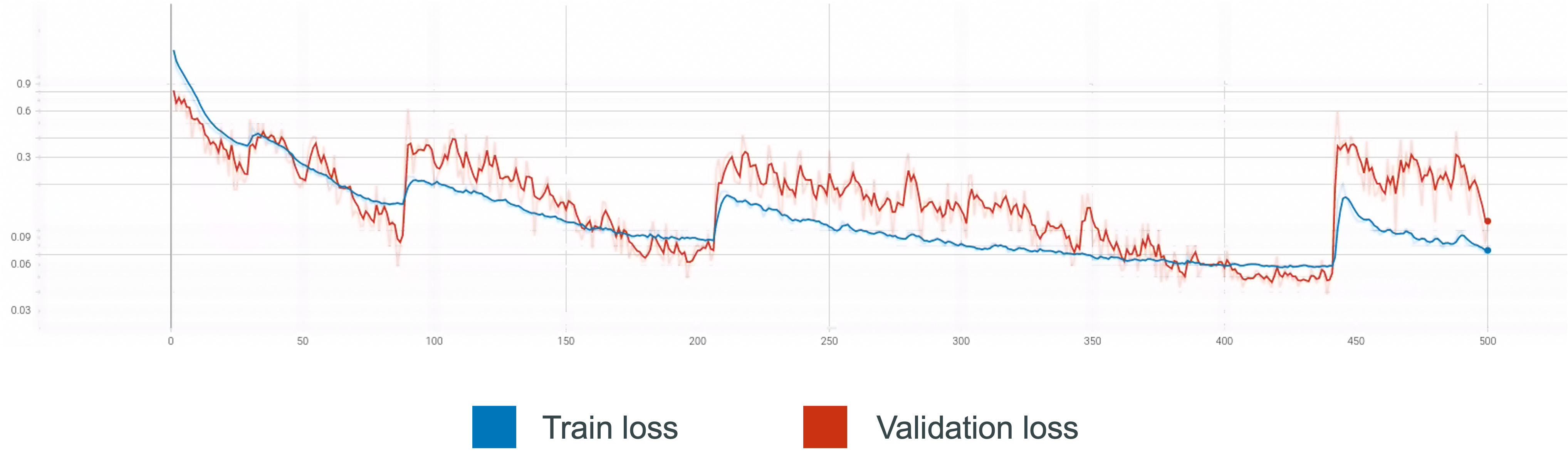
Figure 4. Training and validation loss curves on a logarithmic scale for our DL-based joint inversion. Here, both losses converge, indicating that our proposed joint inversion architecture successfully learns a mapping from our surface gravity and seismic data to 3D subsurface density and velocity models.

6. Results

We train our joint inversion model using the methods described in Section 5. Figure 4 shows the training and validation loss curves on a logarithmic scale. This figure shows that both losses converge, indicating that our proposed joint inversion architecture successfully learns a mapping from our surface gravity and seismic data to 3D subsurface density and velocity models.

In Table 1, we see that our proposed joint inversion generally outperforms gravity and seismic-only inversion for all metrics except for the mean squared error between the observed data and the gravity response of the predicted density model, where the results vs. the gravity only model are comparable. Figure 5 shows a 2D cross-section slice from predictions from each model. Visually, the density models produced by the gravity-only and our joint architectures are similar. However, visual differences exist between the seismic-only reconstructed velocity model and the velocity model produced from our joint architecture (i.e., top right corner); those can also be observed in Figure 6 for a different sample (i.e., at different times of plume’s migration).

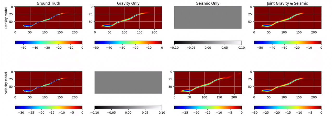
Figure 5. From left to right 2D cross-section slice from ground truth, gravity-only, seismic-only, and joint models. The top row shows density models, and the bottom row shows velocity models. Visually, the density models produced by the gravity-only and our joint architectures are similar. However, visual differences exist between the seismic-only reconstructed velocity model and the velocity model produced from our joint architecture (i.e., top right corner).

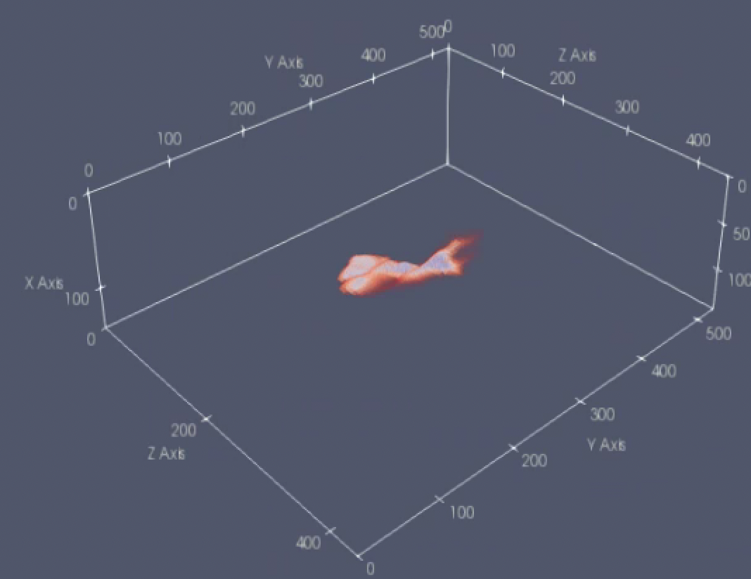
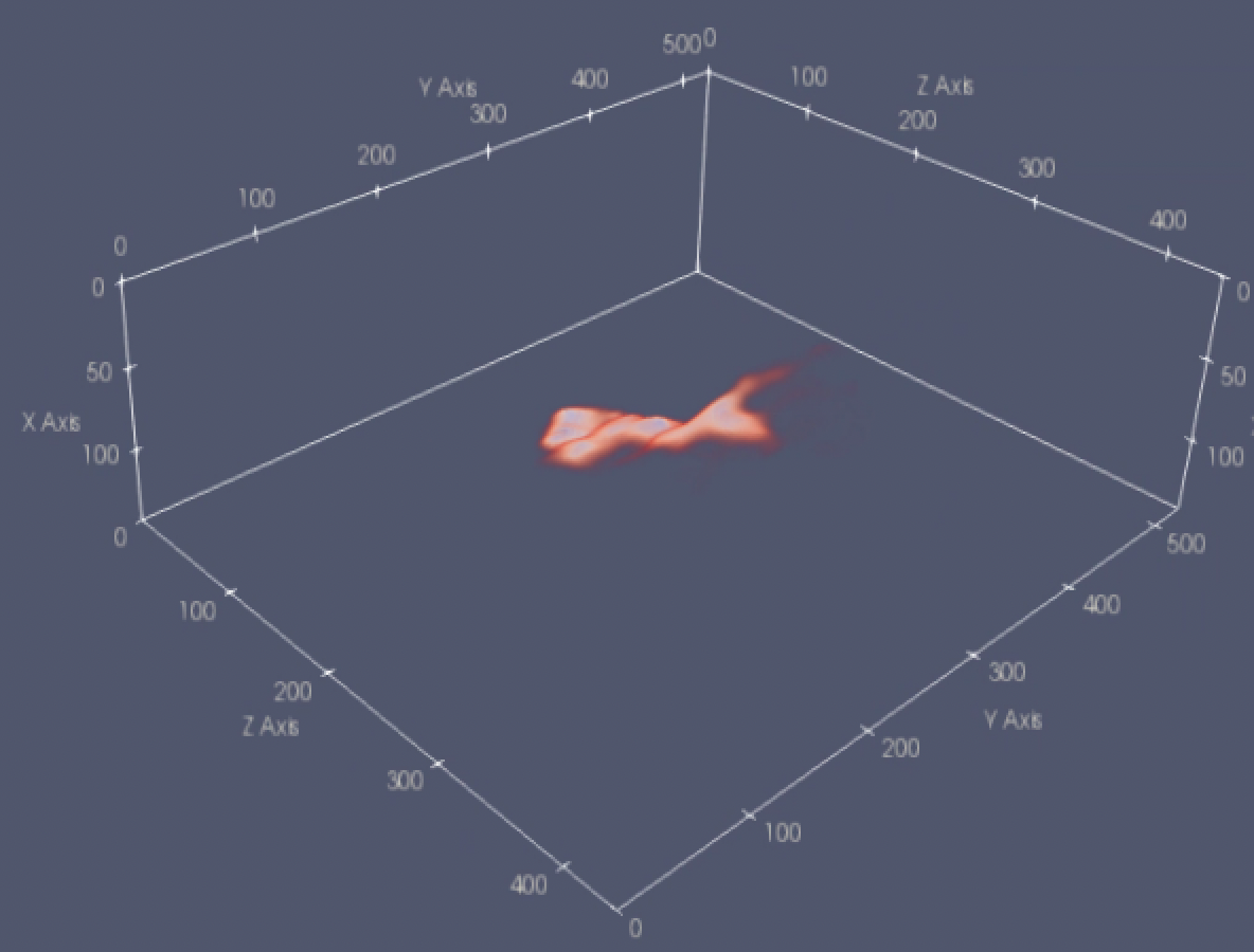
Figure 6. 3D view of label (top) -prediction (bottom) pair of velocity variation given the CO₂ plume location.

7. Discussion

Our results demonstrate the potential benefits of DL-based joint inversion. The joint inversion model consistently outperforms DL-based gravity-only and seismic-only inversion models across various evaluation metrics. This performance suggests that the fusion of surface gravity and seismic data can lead to more accurate subsurface models. The improved performance of the joint inversion model in terms of density and velocity reconstruction, segmentation accuracy, and R-squared coefficients indicates the effectiveness of the proposed approach in capturing the complexity of subsurface CO₂ plumes.

The benefits of DL-based joint inversion are limited from a computational perspective because combining two different datasets requires more memory and time during training. Our joint inversion model takes roughly 45s per epoch on 4 A100 GPUs with a batch size of 8. In contrast, DL-based gravity inversion takes roughly 20s per epoch, and DL-based seismic inversion takes roughly 30s per epoch for the same number of GPUs and batch size. Additionally, joint inversion takes just over 400 epochs to converge to a solution vs. 200 for both the gravity and seismic-only approaches. The greater number of epochs is possibly explained by the more complex relationship our joint inversion approach has to resolve vs. the single mode methods. Regarding inference, our joint model is comparable to the gravity and seismic-only models, producing predictions in less than one second on a single A100 GPU.

We utilize the PocketNet approach proposed by (Celaya et al., 2023a) in our joint architecture. This approach takes advantage of the similarity between the U-Net architecture and geometric multigrid methods to drastically reduce the number of parameters (Celaya et al., 2023a; He and Xu, 2019). Additionally, we replace the transposed convolution with trilinear upsampling. With these modifications, we reduce the number of parameters from roughly 33,000,000 to 349,000, yielding a roughly 40% decrease in the time per epoch. Additionally, these modifications allow us to use a larger batch size (8 instead of 4).

While developing our joint inversion model, we observe that the optimization landscape is tricky, with some local minimums corresponding to good values for density model misfit and R-squared and vice versa for velocity models. Adding a coupling term like in the classical joint inversion formulation given by 2 may help avoid getting trapped in local minimums during training. Future work will focus on formulating and testing a term based on the Dice score. The intuition here is to enforce via our modified loss function that the plumes occupy the same physical space.

Our data comes from simulations of a single geologic formation (Johansen). Further work is needed to test the generalization capability of our joint inversion model to other datasets based on simulations of other CO₂ storage sites (i.e., Snohvit and Kimberlina (Alumbaugh et al., 2023)) and on field data. However, time-lapse CCUS monitoring with gravity (and other non-seismic methods) is a data-poor field. Sufficiently detailed reservoir models for CCUS, especially field data, are hard to come by, and access is limited (Celaya et al., 2023b; Alumbaugh et al., 2023).

8. Conclusions

We developed an effective DL-based joint inversion method to recover high-resolution, subsurface CO₂ density and velocity models from surface gravity and seismic data. We train our joint DL architecture on realistic, physics-simulated CO₂ plumes, surface gravity, and seismic data. This training approach mirrors real-world site data collection. Our joint inversion outperforms gravity and seismic-only inversion techniques for our selected metrics. While there is room for improvement, the results presented here are promising and represent, to the best of our knowledge, the first fully 3D DL-based joint inversion of surface gravity and seismic data derived from a physics simulation of a proposed CO₂ storage site.

- (1)
- Adler et al. (2021) Amir Adler, Mauricio Araya-Polo, and Tomaso Poggio. 2021. Deep Learning for Seismic Inverse Problems: Toward the Acceleration of Geophysical Analysis Workflows. IEEE Signal Processing Magazine 38, 2 (2021), 89–119. https://doi.org/10.1109/MSP.2020.3037429
- Alumbaugh et al. (2023) David Alumbaugh, Erika Gasperikova, Dustin Crandall, Michael Commer, Shihang Feng, William Harbert, Yaoguo Li, Youzuo Lin, and Savini Samarasinghe. 2023. The Kimberlina synthetic multiphysics dataset for CO2 monitoring investigations. Geoscience Data Journal (2023).
- Alyousuf et al. (2022) Taqi Alyousuf, Yaoguo Li, and Richard Krahenbuhl. 2022. Machine learning inversion of time-lapse three-axis borehole gravity data for CO2 monitoring. 3099–3103. https://doi.org/10.1190/image2022-3745388.1 arXiv:https://library.seg.org/doi/pdf/10.1190/image2022-3745388.1
- Araya-Polo et al. (2018) Mauricio Araya-Polo, Joseph Jennings, Amir Adler, and Taylor Dahlke. 2018. Deep-learning tomography. The Leading Edge 37, 1 (2018), 58–66. https://doi.org/10.1190/tle37010058.1 arXiv:https://doi.org/10.1190/tle37010058.1
- Bakas et al. (2018) Spyridon Bakas et al. 2018. Identifying the best machine learning algorithms for brain tumor segmentation, progression assessment, and overall survival prediction in the BRATS challenge. arXiv preprint arXiv:1811.02629 (2018).
- Boulanger and Chouteau (2001) O. Boulanger and M. Chouteau. 2001. Constraints in 3D gravity inversion. Geophysical Prospecting 49, 2 (2001), 265–280. https://doi.org/10.1046/j.1365-2478.2001.00254.x
- Celaya et al. (2023a) Adrian Celaya, Jonas A. Actor, Rajarajesawari Muthusivarajan, Evan Gates, Caroline Chung, Dawid Schellingerhout, Beatrice Riviere, and David Fuentes. 2023a. PocketNet: A Smaller Neural Network for Medical Image Analysis. IEEE Transactions on Medical Imaging 42, 4 (2023), 1172–1184. https://doi.org/10.1109/TMI.2022.3224873
- Celaya et al. (2023b) Adrian Celaya, Bertrand Denel, Yen Sun, Mauricio Araya-Polo, and Antony Price. 2023b. Inversion of Time-Lapse Surface Gravity Data for Detection of 3-D CO2 Plumes via Deep Learning. IEEE Transactions on Geoscience and Remote Sensing 61 (2023), 1–11. https://doi.org/10.1109/TGRS.2023.3273149
- Chen et al. (2020) Jie Chen, Cara Schiek-Stewart, Ligang Lu, Susanne Witte, Karin Eres Guardia, Francesco Menapace, Pandu Devarakota, and Mohamed Sidahmed. 2020. Machine learning method to determine salt structures from gravity data. In SPE Annual Technical Conference and Exhibition. OnePetro.
- Colombo et al. (2020) Daniele Colombo, Weichang Li, Ernesto Sandoval-Curiel, and Gary W. McNeice. 2020. Deep-learning electromagnetic monitoring coupled to fluid flow simulators. GEOPHYSICS 85, 4 (2020), WA1–WA12. https://doi.org/10.1190/geo2019-0428.1 arXiv:https://doi.org/10.1190/geo2019-0428.1
- De Groot-Hedlin and Constable (1990) Catherine De Groot-Hedlin and SC Constable. 1990. OCCAM’s inversion to generate smooth, two-dimensional models from magnetotelluric data. GEOPHYSICS 55 (12 1990), 1613–1624. https://doi.org/10.1190/1.1442813
- Deng et al. (2009) Jia Deng, Wei Dong, Richard Socher, Li-Jia Li, Kai Li, and Li Fei-Fei. 2009. ImageNet: A large-scale hierarchical image database. In 2009 IEEE Conference on Computer Vision and Pattern Recognition. 248–255. https://doi.org/10.1109/CVPR.2009.5206848
- Eigestad et al. (2009) G. Eigestad, Helge Dahle, Bjarte Hellevang, Fridtjof Riis, Wenche Johansen, and Erlend Øian. 2009. Geological modeling and simulation of CO2 injection in the Johansen formation. Computational Geosciences 13 (12 2009), 435–450. https://doi.org/10.1007/s10596-009-9153-y
- Fawad and Mondol (2021) Manzar Fawad and Nazmul Haque Mondol. 2021. Monitoring geological storage of CO2: A new approach. Scientific Reports 11, 1 (2021), 5942.
- Gelboim et al. (2022) Maayan Gelboim, Amir Adler, Yen Sun, and Mauricio Araya-Polo. 2022. Encoder–Decoder Architecture for 3D Seismic Inversion. Sensors 23, 1 (2022), 61.
- He and Xu (2019) Juncai He and Jinchao Xu. 2019. MgNet: A unified framework of multigrid and convolutional neural network. Science china mathematics 62 (2019), 1331–1354.
- Hoek and Bray (1981) Evert Hoek and Jonathan D Bray. 1981. Rock slope engineering. CRC press.
- Hu et al. (2023) Yanyan Hu, Xiaolong Wei, Xuqing Wu, Jiajia Sun, Jiuping Chen, Yueqin Huang, and Jiefu Chen. 2023. A deep learning-enhanced framework for multiphysics joint inversion. GEOPHYSICS 88, 1 (2023), K13–K26. https://doi.org/10.1190/geo2021-0589.1 arXiv:https://doi.org/10.1190/geo2021-0589.1
- Huang et al. (2021) Rui Huang, Shuang Liu, Rui Qi, and Yujie Zhang. 2021. Deep Learning 3D Sparse Inversion of Gravity Data. Journal of Geophysical Research: Solid Earth 126, 11 (2021), e2021JB022476.
- Jin et al. (2017) Kyong Hwan Jin, Michael T. McCann, Emmanuel Froustey, and Michael Unser. 2017. Deep Convolutional Neural Network for Inverse Problems in Imaging. IEEE Transactions on Image Processing 26, 9 (2017), 4509–4522. https://doi.org/10.1109/TIP.2017.2713099
- Karras et al. (2019) Tero Karras, Samuli Laine, and Timo Aila. 2019. A style-based generator architecture for generative adversarial networks. In Proceedings of the IEEE/CVF conference on computer vision and pattern recognition. 4401–4410.
- Kim and Nakata (2018) Yuji Kim and Nori Nakata. 2018. Geophysical inversion versus machine learning in inverse problems. The Leading Edge 37, 12 (2018), 894–901. https://doi.org/10.1190/tle37120894.1 arXiv:https://doi.org/10.1190/tle37120894.1
- Kingma and Ba (2014) Diederik P Kingma and Jimmy Ba. 2014. Adam: A method for stochastic optimization. arXiv preprint arXiv:1412.6980 (2014).
- Lelièvre et al. (2012) Peter G Lelièvre, Colin G Farquharson, and Charles A Hurich. 2012. Joint inversion of seismic traveltimes and gravity data on unstructured grids with application to mineral exploration. Geophysics 77, 1 (2012), K1–K15.
- Li et al. (2020) Shucai Li, Bin Liu, Yuxiao Ren, Yangkang Chen, Senlin Yang, Yunhai Wang, and Peng Jiang. 2020. Deep-Learning Inversion of Seismic Data. IEEE Transactions on Geoscience and Remote Sensing 58, 3 (2020), 2135–2149. https://doi.org/10.1109/TGRS.2019.2953473
- Li and Oldenburg (1998) Yaoguo Li and Douglas W. Oldenburg. 1998. 3-D inversion of gravity data. GEOPHYSICS 63, 1 (1998), 109–119. https://doi.org/10.1190/1.1444302 arXiv:https://doi.org/10.1190/1.1444302
- Liu et al. (2020) Bin Liu et al. 2020. Deep Learning Inversion of Electrical Resistivity Data. IEEE Transactions on Geoscience and Remote Sensing 58, 8 (2020), 5715–5728. https://doi.org/10.1109/TGRS.2020.2969040
- Loshchilov and Hutter (2017) Ilya Loshchilov and Frank Hutter. 2017. SGDR: Stochastic Gradient Descent with Warm Restarts. In International Conference on Learning Representations. https://openreview.net/forum?id=Skq89Scxx
- Milletari et al. (2016) Fausto Milletari, Nassir Navab, and Seyed-Ahmad Ahmadi. 2016. V-net: Fully convolutional neural networks for volumetric medical image segmentation. In 2016 fourth international conference on 3D vision (3DV). IEEE, 565–571.
- Moorkamp et al. (2011) Max Moorkamp, Björn Heincke, Marion Jegen, Alan W Roberts, and Richard W Hobbs. 2011. A framework for 3-D joint inversion of MT, gravity and seismic refraction data. Geophysical Journal International 184, 1 (2011), 477–493.
- Nabighian et al. (2005) MN Nabighian, VJS Grauch, RO Hansen, TR LaFehr, Y Li, JW Peirce, JD Phillips, and ME Ruder. 2005. 75th Anniversary. The historical development of the magnetic method in exploration: Geophysics 70, 6 (2005).
- Oh et al. (2020) Seokmin Oh, Kyubo Noh, Soon Jee Seol, and Joongmoo Byun. 2020. Cooperative deep learning inversion of controlled-source electromagnetic data for salt delineation. GEOPHYSICS 85, 4 (2020), E121–E137.
- Pariseau (2017) William G Pariseau. 2017. Design analysis in rock mechanics. CRC Press.
- Paszke et al. (2019) Adam Paszke, Sam Gross, Francisco Massa, Adam Lerer, James Bradbury, Gregory Chanan, Trevor Killeen, Zeming Lin, Natalia Gimelshein, Luca Antiga, Alban Desmaison, Andreas Köpf, Edward Z. Yang, Zach DeVito, Martin Raison, Alykhan Tejani, Sasank Chilamkurthy, Benoit Steiner, Lu Fang, Junjie Bai, and Soumith Chintala. 2019. PyTorch: An Imperative Style, High-Performance Deep Learning Library. CoRR abs/1912.01703 (2019). arXiv:1912.01703 http://arxiv.org/abs/1912.01703
- Rezaie et al. (2017) Mohammad Rezaie, Ali Moradzadeh, and Ali Nejati Kalateh. 2017. Fast 3D inversion of gravity data using solution space priorconditioned lanczos bidiagonalization. Journal of Applied Geophysics 136 (2017), 42–50. https://doi.org/10.1016/j.jappgeo.2016.10.019
- Shahriari et al. (2020) Mostafa Shahriari, David Pardo, Artzai Picón, Adrian Galdran, Javier Del Ser, and Carlos Torres-Verdín. 2020. A deep learning approach to the inversion of borehole resistivity measurements. Computational Geosciences 24, 3 (2020), 971–994.
- Sudre et al. (2017) Carole H. Sudre, Wenqi Li, Tom Kamiel Magda Vercauteren, Sébastien Ourselin, and M. Jorge Cardoso. 2017. Generalised Dice Overlap as a Deep Learning Loss Function for Highly Unbalanced Segmentations. In Deep Learning in Medical Image Analysis and Multimodal Learning for Clinical Decision Support. Springer International Publishing, 240–248.
- Sun et al. (2020) Yen Sun, Bertrand Denel, Norman Daril, Lory Evano, Paul Williamson, and Mauricio Araya-Polo. 2020. Deep learning joint inversion of seismic and electromagnetic data for salt reconstruction. SEG Technical Program Expanded Abstracts 2020 (2020), 550–554. https://doi.org/10.1190/segam2020-3426925.1 arXiv:https://library.seg.org/doi/pdf/10.1190/segam2020-3426925.1
- Sundal et al. (2016) Anja Sundal, Johan Petter Nystuen, Kari-Lise Rørvik, Henning Dypvik, and Per Aagaard. 2016. The Lower Jurassic Johansen Formation, northern North Sea – Depositional model and reservoir characterization for CO2 storage. Marine and Petroleum Geology 77 (2016), 1376–1401. https://doi.org/10.1016/j.marpetgeo.2016.01.021
- Tarantola and Valette (1981) Albert Tarantola and Bernard Valette. 1981. Inverse problems = Quest for information. Journal of Geophysics 50, 1 (October 1981), 159–170.
- Um et al. (2022) Evan Schankee Um, David Alumbaugh, Michael Commer, Shihang Feng, Erika Gasperikova, Yaoguo Li, Youzuo Lin, and Savini Samarasinghe. 2022. Deep-learning multiphysics network for imaging CO2 saturation and estimating uncertainty in geological carbon storage. Geophysical Prospecting (2022). https://doi.org/10.1111/1365-2478.13257 arXiv:https://onlinelibrary.wiley.com/doi/pdf/10.1111/1365-2478.13257
- Yang and Ma (2019) Fangshu Yang and Jianwei Ma. 2019. Deep-learning inversion: A next-generation seismic velocity model building method. GEOPHYSICS 84, 4 (2019), R583–R599. https://doi.org/10.1190/geo2018-0249.1 arXiv:https://doi.org/10.1190/geo2018-0249.1
- Yang et al. (2022) Qianguo Yang, Xiangyun Hu, Shuang Liu, Qu Jie, Huaijiang Wang, and Qiuhua Chen. 2022. 3-D Gravity Inversion Based on Deep Convolution Neural Networks. IEEE geoscience and remote sensing letters 19 (2022), 1–5.
- Yu-Feng et al. (2021) Wang Yu-Feng, Zhang Yu-Jie, Fu Li-Hua, and Li Hong-Wei. 2021. Three-dimensional gravity inversion based on 3D U-Net++. Applied Geophysics 18, 4 (2021), 451–460.