Abstract

In this research study, the focus is on exploring the influence of topological effects in the presence of a hot-dense medium. To achieve this, we solve the non-relativistic Schrödinger wave equation while considering the quantum flux field and its interaction potential. By doing so, we are able to obtain the energy eigenvalues and corresponding wave functions by using the Nikiforov-Uvarov method. The findings reveal that when taking into account both topological effects and the magnetic flux $\Phi$, there is a reduction in the binding energy in the hot-dense medium. Furthermore, we examine the role of the baryonic potential on the binding energy in the $(T,u_{b})$ plane. It is observed that the effect of the baryonic potential is more pronounced when its values are smaller.

Impact of Global Monopoles on Heavy Mesons in a Hot-Dense Medium

Keywords: Topological effects; Schrödinger equation; Nikiforov-Uvarov method; Finite temperature; Baryonic chemical potential

1 Introduction

The investigation of strongly interacting matter in extreme conditions has become a subject of great interest due to its relevance to particle physics and astrophysics. One specific area of importance is studying how the properties of hadrons, such as their masses, magnetic moments, and decay constants, can be altered when they propagate through a hot medium. Understanding the behavior of quarks and gluons in this hot medium, known as quark-gluon plasma (QGP), requires a thorough examination of hadron properties at finite temperature and density. The exploration of this phase, the QGP, is being conducted in experiments at RHIC (Brookhaven National Laboratory) and CERN, where there is substantial evidence supporting its existence [1]. Numerous studies have been conducted on this topic, employing both relativistic and non-relativistic quark models as detailed in references [2, 3, 4, 5, 6, 7, 8, 9, 10, 11, 12].

In Ref. [2], the analytical solution of the N-radial Schrodinger equation is obtained by extending the Cornell potential to finite temperature. This study aims to investigate the behavior of charmonium and bottomonium masses at finite temperature. In Ref. [3], the dissociation of quarkonia (bound states of quarks and antiquarks) in a thermal quantum chromodynamics medium is studied by using the conformable fractional of the Nikiforov–Uvarov (CF–NU) method. This study aims to understand how the thermal environment affects the stability of quarkonia states.

Ref. [4] focuses on the thermodynamic properties of heavy mesons. These properties are calculated using the N-dimensional radial Schrodinger equation. Ref. [5] presents an analytical study of the N-radial Schrodinger equation using the supersymmetric quantum mechanics method. In this study, the heavy-quarkonia potential is introduced at finite temperature and baryon chemical potential to investigate its effects on the system. Moreover, the dissociation of quarkonia is investigated in an anisotropic plasma within hot and dense media in Refs. [6, 7, 8]. These studies aim to understand how the anisotropic nature of the plasma influences the behavior of quarkonia.

The quark sigma model, a relativistic quark model, has emerged as a valuable tool in comprehending strong nuclear interactions [9, 10]. Within this model, the phenomenon of spontaneous chiral symmetry breaking and its restoration at higher temperatures are demonstrated. Numerous researchers have explored the Hartree approximation of the linear sigma model employing two or four quark flavors, investigating its behavior at different temperature regimes [1, 11, 12, 13, 14, 15]. Furthermore, several studies have successfully applied the quark sigma model to characterize both static and dynamic baryons at various temperatures and densities, as documented in references [16, 17, 18]. This demonstrates the model’s versatility in describing the properties of baryons under diverse thermodynamic conditions.

Topological defects are fascinating and exotic objects that are believed to have formed during phase transitions in the early universe. They are intriguing phenomena that arise in various physical systems and have been extensively studied in the context of quantum mechanics, atomic and molecular physics, and condensed matter physics. The different types of topological defects known in the literature include cosmic strings, domain walls, global monopoles, and textures, among others. Each of these defects exhibits unique properties and characteristics that make them significant in understanding fundamental aspects of physics. Cosmic strings are long, thin, and stable one-dimensional defects that are hypothesized to have formed when the universe underwent a phase transition. These strings are thought to play a crucial role in the large-scale structure of the cosmos, influencing the distribution of matter and galaxies.

Global monopoles are three-dimensional spherical objects that are the result of spontaneous symmetry breaking in certain grand unified theories. They have interesting properties related to their mass and interaction, and they can influence the evolution of the universe on cosmological scales. The study of topological defects has led to deep insights into various aspects of physics and has provided valuable connections between different fields. Their presence and behavior have implications for the early universe, as well as condensed matter systems and atomic and molecular interactions.

In this study, our objective is to investigate the influence of topological effects and magnetic flux in a hot-dense medium on heavy mesons. To achieve this, we solve the radial Schrödinger equation using the Nikiforov-Uvarov method [19], obtaining the energy eigenvalues and corresponding wave functions. To the best of our knowledge, the impact of topological effects on heavy mesons in a hot-dense medium has not been adequately considered in previous research, making this study a significant contribution to the field.

The paper is organized as follows: In the introduction, the context and motivation of the study are presented. Section 2 elaborates on the Nikiforov-Uvarov method, providing readers with a clear understanding of the mathematical approach used in the research. The subsequent Section 3 outlines the details of the energy eigenvalues and wave functions calculation. Section 4 engages in a comprehensive discussion of the obtained results, interpreting and analyzing the implications of the topological effects and magnetic flux in a hot-dense medium on heavy mesons. Finally, Section 5 summarizes the key findings and presents concluding remarks, underscoring the significance of the study and potential avenues for further research.

2 Theoretical Description of the Nikiforov-Uvarov (NU) Method

In this section, we will present a concise overview of the NU method [19], which serves as a valuable tool for solving second-order differential equations in the specified form given by

$$\Psi^{\prime\prime}(s)+\frac{\bar{\tau}(s)}{\sigma(s)}\Psi^{\prime}(s)+\frac{\tilde{\sigma}(s)}{\sigma^{2}(s)}\Psi(s)=0,$$ (1)

where $\sigma(s)$ and $\tilde{\sigma}(s)$ are polynomials of maximum second degree and $\bar{\tau}(s)$ is a polynomial of maximum first degree with an appropriate $s=s(r)$ coordinate transformation. To find particular solution of Eq. (1) by separation of variables, if one deals with the transformation

$$\Psi(s)=\Phi(s)\chi(s),$$ (2)

it reduces to an equation of hypergeometric type as follows

$$\sigma(s)\chi^{\prime\prime}(s)+\tau(s)\chi^{\prime}(s)+\lambda\chi(s)=0,$$ (3)

where

$$\sigma(s)=\pi(s)\frac{\Phi(s)}{\Phi^{\prime}(s)},$$ (4)

$$\tau(s)=\bar{\tau}(s)+2\pi(s);~{}\ \ \tau^{\prime}(s)<0,$$ (5)

and

$$\lambda=\lambda_{n}=-n\tau^{\prime}(s)-\frac{n(n-1)}{2}\sigma^{\prime\prime}(s),n=0,1,2,...$$ (6)

$\chi(s)=\chi_{n}(s)$ which is a polynomial of $n$ degree which satisfies the hypergeometric equation, taking the following form

$$\chi_{n}(s)=\frac{B_{n}}{\rho_{n}}\frac{d^{n}}{ds^{n}}(\sigma^{\prime\prime}(s)\rho(s)),$$ (7)

where $B_{n}$ is a normalization constant and $\rho(s)$ is a weight function which satisfies the following equation

$$\frac{d}{ds}\omega(s)=\frac{\tau(s)}{\sigma(s)}\omega(s);\ \ \ \omega(s)=\sigma(s)\rho(s),$$ (8)

$$\pi(s)=\frac{\sigma^{\prime}(s)-\bar{\tau}(s)}{2}\pm\sqrt{(\frac{\sigma^{\prime}(s)-\bar{\tau}(s)}{2})^{2}-\tilde{\sigma}(s)+K\sigma(s),}$$ (9)

and

$$\lambda=K+\pi^{\prime}(s),$$ (10)

the $\pi(s)$ is a polynomial of first degree. The values of $K$ in the square-root of Eq. (9) is possible to calculate if the expressions under the square root are square of expressions. This is possible if its discriminate is zero. (for detail, see Ref. [19]).

3 The Schrödinger Equation in point-like Global Monopole with potential interaction

In this section, we delve into the analysis of the eigenvalues for non-relativistic particles under the influence of a quantum flux field, taking into account the presence of a point-like global monopole with a potential. We employ the NU-method to solve the radial equation, enabling us to obtain the necessary solutions.

Furthermore, our investigation involves a comprehensive examination of the influence of several critical factors, such as the topological defect and the magnetic flux, particularly in the context of a hot and/or dense medium. By considering these factors, we aim to gain valuable insights into the behavior and properties of the system, shedding light on the intricate interplay between quantum flux, topological defects, and thermodynamic conditions.

For a detailed explanation of the two-particle system interacting through an electromagnetic spherically symmetric potential $V(r)$, see Ref. [20, 21, 22, 23, 24, 25, 26, 27, 28, 29]

$$\Bigg{[}\frac{d^{2}}{dr^{2}}+\frac{1}{\alpha^{2}}\Big{\{}2\,\mu\,(E-V(r))-\frac{\ell^{\prime}(\ell^{\prime}+1)}{r^{2}}\Big{\}}\Bigg{]}\,\Psi(r)=0,$$ (11)

where $\ell^{\prime}=(|m-\Phi|+\kappa)$ with $\kappa=0,1,2,3,...$, $m$ is the magnetic quantum number, $\ell$ is the angular momentum quantum number, $\mu$ is the reduced mass for the quarkonium particle (for charmonium $\mu=\frac{m_{c}}{2}$ and for bottomonium $\mu=\frac{m_{b}}{2}$), respectively, and $0<\alpha<1$ characterise the topological defect parameter of point-like global monopole, and $\Phi$ is the amount of magnetic flux which is a positive real number.

At finite temperature, the potential interaction can given as [30] as follows

$$V(r)=a\,\left(m_{D},r\right)\,r-\frac{b\left(m_{D},r\right)}{r},$$ (12)

where $a\left(T,r\right)=\frac{a}{m_{D}(T)\,r}\,\Big{(}1-e^{-m_{D}\,r}\Big{)}$ and $b\left(T,r\right)=b\,e^{-m_{D}\,r}$ where $m_{D}\left(T,u_{q}\right)$ is the Debye mass that vanishes at $T\to 0$ and $a$ and $b$ are arbitrary constants will be determined later (for detail, see Ref. [30]). By substituting Eq. (2) into Eq. (1) and using approximation $e^{-m_{D}\left(T\right)r}={\displaystyle\sum\limits_{j=0}^{\infty}}\frac{\left(-m_{D}\left(T\right)r\right)^{j}}{j!}$ up to second-order, which gives a good accuracy when $m_{D}r\ll 1$. We obtain

$$\Bigg{[}\frac{d^{2}}{dr^{2}}+2\mu^{\prime}(E-A+\frac{b}{r}-Cr+Dr^{2}-\frac{\ell^{\prime}(\ell^{\prime}+1)}{2\,\mu\,r^{2}})\Bigg{]}\,R(r)=0,$$ (13)

where, $A=b~{}m_{D}\left(T\right),C=a-\frac{1}{2}bm_{D}^{2}\left(T\right)$, $D=\frac{1}{2}a~{}m_{D}\left(T\right)$, and $\mu^{\prime}=\frac{\mu}{\alpha}$

By taking $r=\frac{1}{x}$, Eq. (13) takes the following form

$$\Bigg{[}\frac{d^{2}}{dx^{2}}+\frac{2}{x}\frac{d}{dx}+\frac{2\,\mu^{\prime}}{x^{4}}\Big{(}E-A+bx-\frac{C}{x}+\frac{D}{x^{2}}-\frac{\ell^{\prime}(\ell^{\prime}+1)}{2\mu}x\Big{)}\Bigg{]}\,R(x)=0.$$ (14)

The scheme is based on the expansion of $\frac{C}{x}$ and $\frac{D}{x^{2}}$ in a power series around the characteristic radius $r_{0}$ of meson up to the second order. Setting $y=x-\delta$, where $\delta=\frac{1}{r_{0}}$, thus, we expand the $\frac{c}{x}$ and $\frac{D}{x^{2}}$ into a series of powers around $y=0$.

$$\frac{C}{x} =\frac{C}{y+\delta}=\frac{1}{\delta}(1+\frac{y}{\delta})^{-1}$$

$$=\frac{C}{\delta}(1-\frac{y}{\delta}+\frac{y}{\delta^{2}}),$$

$$=C(\frac{3}{\delta}-\frac{3x}{\delta^{2}}+\frac{x^{2}}{\delta^{3}})\text{.}$$ (15)

Similarly,

$$\frac{D}{x^{2}}=D(\frac{6}{\delta^{2}}-\frac{8x}{\delta^{3}}+\frac{3x^{2}}{\delta^{4}})\text{.}$$ (16)

By substituting Eqs. (15 and 16) into Eq. (14). Eq. (14) takes the following form

$$\Bigg{[}\frac{d^{2}}{dx^{2}}+\frac{2}{x}\frac{d}{dx}+\frac{2\mu^{\prime}}{x^{4}}(-A_{1}+A_{2}x-A_{3}x^{2})\Bigg{]}\,R(x)=0,$$ (17)

where, $A_{1}=-(E-A-\frac{3C}{\delta}+\frac{6D}{\delta^{2}})$, $A_{2}=(\frac{3C}{\delta^{2}}-\frac{8D}{\delta^{3}}+b)$, and $A_{3}=(\frac{C}{\delta^{3}}-\frac{3D}{\delta^{4}}+\frac{\ell^{\prime}\,(\ell^{\prime}+1)}{2\mu})$.  The $\frac{1}{x}$ expansion gives a good accuracy when $\delta$ tends to $x$.

By comparing Eq. (17) and Eq. (1), we find $\bar{\tau}(s)=2x$, $\sigma(s)=x^{2}$, and $\tilde{\sigma}(s)=2\mu^{\prime}(-A_{1}+A_{2}x-A_{3}x^{2})$. Hence, the Eq. (17) satisfies the conditions in Eq. (1). By following the NU method that mentioned in Sec. 2, therefore

$$\pi=\pm\sqrt{\left(K+2A_{3}\right)x^{2}-2A_{2}x+2A_{1}}.$$ (18)

The constant $K$ is chosen such as the function under the square root has a double zero, i.e. its discriminant $\Delta=4A_{2}^{2}-8A_{1}\left(K+2A_{3}\right)=0$. Hence,

$$\pi=\pm\frac{1}{\sqrt{2A_{1}}}\left(2A_{1}-A_{2}x\right)\text{.}$$ (19)

Thus,

$$\tau=2x\pm\frac{1}{\sqrt{2A_{1}}}\left(2A_{1}-A_{2}x\right)\text{.}$$ (20)

For bound state solutions, we choose the positive sign in above equation so that the derivative

$$\tau^{\prime}=2-\frac{2A_{2}}{\sqrt{2A_{1}}}\text{.}$$ (21)

By using Eq. (10), we obtain

$$\lambda=\frac{A_{2}^{2}}{2A_{1}}-2A_{3}-\frac{A_{2}}{\sqrt{2A_{1}}},$$ (22)

and Eq. (6), we obtain

$$\lambda_{n}=-n\left(2-\frac{2A_{2}}{\sqrt{2A_{1}}}\right)-n(n-1)\text{.}$$ (23)

From Eq. (6); $\lambda=\lambda_{n}$. The energy eigenvalues of Eq. (13) in the hot-dense medium is given

$$E_{n\,\ell}^{N}=A+\frac{3C}{\delta}-\frac{6D}{\delta^{2}}-\frac{2\mu^{\prime}(\frac{3C}{\delta^{2}}+b-\frac{8~{}D}{\delta^{3}})^{2}}{\Big{[}(2n+1)\pm\sqrt{1+\frac{8\mu^{\prime}C}{\delta^{3}}+\frac{4}{\alpha}\,\ell^{\prime}(\ell^{\prime}+1)-\frac{24\mu^{\prime}D}{\delta^{4}}}\Big{]}^{2}}.$$ (24)

The radial of wave function of Eq. (13) takes the following form

$$R_{n\,\ell}\left(r\right)=C_{n\,\ell}~{}r^{-\frac{A_{2}}{\sqrt{2A_{1}}}-1}e^{\sqrt{2A_{1}}\,r}(-r^{2}\frac{d}{d\,r})^{n}(r^{-2n+\frac{A_{2}}{\sqrt{2A_{1}}}}e^{-2\sqrt{2A_{1}}r}).$$ (25)

$C_{nL}$ is the normalization constant that is determined  by $\int\left|R_{nL}\left(r\right)\right|^{2}dr=1$.

4 Discussion of Results

In this section, we calculate spectra of the heavy quarkonium system such as bottomonium mesons in the hot and dense madium. The mass of quarkonium is calculated in the 3-dimensional space. We apply the following relation as in Ref. [2]

$$M=2\,m+E_{n\ell},$$ (26)

where $m$ is quarkonium bare mass for the charmonium or bottomonium mesons. By using Eq. (24), we write Eq. (26) as follows:

$$M=2m+A+\frac{3C}{\delta}-\frac{6D}{\delta^{2}}-\frac{2\mu^{\prime}(\frac{3C}{\delta^{2}}+b-\frac{8~{}D}{\delta^{3}})^{2}}{\Big{[}(2n+1)\pm\sqrt{1+\frac{8\mu^{\prime}C}{\delta^{3}}+\frac{4}{\alpha}\ell^{\prime}(\ell^{\prime}+1)-\frac{24\mu^{\prime}D}{\delta^{4}}}\Big{]}^{2}}$$ (27)

Eq. (27) represents the quarkonium masses in hot and dense medium with topological effects and magnetic flux. By taking $\alpha=1$and $\Phi=0,$ we obtain

$$M=2m+A+\frac{3C}{\delta}-\frac{6D}{\delta^{2}}-\frac{2\mu(\frac{3C}{\delta^{2}}+b-\frac{8~{}D}{\delta^{3}})^{2}}{\Big{[}(2n+1)\pm\sqrt{1+\frac{8\mu C}{\delta^{3}}+4\ell(\ell+1)-\frac{24\mu D}{\delta^{4}}}\Big{]}^{2}}$$ (28)

Eq. (28) coincides with the result obtained in Ref. $\left[2\right]$.

We can obtain the quarkonium masses at classical case by taking $T=0$ leads to $A=D=0$ and $C=a$, and $\alpha=1$and $\Phi=0,$Therefore, Eq. (27) takes the following form

$$M=2m+\frac{3a}{\delta}-\frac{2\mu(\frac{3a}{\delta^{2}}+b)^{2}}{\Big{[}(2n+1)\pm\sqrt{1+\frac{8\mu a}{\delta^{3}}+4\ell(\ell+1)}\Big{]}^{2}}.$$ (28)

Eq. (28) coincides with the result obtained in Ref. [31]. In the present work, the Debye mass $D(T,\mu_{b})$ is given in Refs. [32, 33]

$$D(T,\mu_{b})=gT\sqrt{\frac{N_{c}}{3}+\frac{N_{f}}{6}+\frac{N_{f}}{2\pi^{2}}\left(\frac{\mu_{q}}{T}\right)^{2}},$$ (29)

where, $g$  is the coupling constant as defined in Ref. [34], $\mu_{q}$ is the quark chemical potential $\left(\mu_{q}=\frac{\mu_{b}}{3}\right)$, $N_{f}$  is number of flavours, and $N_{c}$ is number of colors.

For the bottomonium meson, the binding energy is plotted as a ratio of temperature ($\frac{T}{T_{a}}$) where $T_{a}$ is a critical temperature in Fig. (1). This plot is done when the baryonic chemical potential is not considered. It is observed that the binding energy decreases as the temperature increases. This behavior is similar for different values of the magnetic flux ($\Phi$). When the magnetic flux ($\Phi$) is decreased, the curves on the plot shift to higher values. Furthermore, the effect of temperature is more significant at the critical temperature ($T_{a}=0.17$ GeV). As the temperature increases beyond this critical temperature, the effect of magnetic flux ($\Phi$) becomes less pronounced in Fig. 2

The authors of Ref. [2] considered the topological effects without considering the hot-dense medium. They found that the potential energy is shifted to higher values with increasing values of magnetic flux ($\Phi$) or the parameter $\alpha$, which is consistent with our findings.

Fig. 3 shows the binding energy plotted for different values of $\alpha$ without considering the baryonic chemical potential ($u_{b}=0$). It is noted that the binding energy reaches its maximum when the topological effects are ignored at $\alpha=1$. Additionally, the effect of topological effects on the binding energy is observed to be dependent on the value of $\alpha$. The curves in Fig. 3 are shifted from each other when topological effects are considered at $\alpha=0.25$.

Overall, these findings suggest that the topological effects, magnetic flux ($\Phi$), and parameter $\alpha$ have significant impacts on the binding energy of the bottomonium meson in different temperature regimes, as illustrated above.

In Fig. 4, we plotted the binding energy as a function of ratio of temperature and the baryonic chemical potential, in which we study the effect of dense medium on the binding energy in the hot medium. When ignored the effect of topological effects at $\alpha=1$ with magnetic flux $\Phi=0.25,$ we note that the binding energy decreases with increasing the temperature at any value of the baryonic chemical potential. Additionally, the binding energy decreases slowly by increasing baryonic chemical potential. Therefore, we deduced that the effect of hot medium is more effect on the binding energy of bottomonium. In Fig. 5, we consider the topological effects at $\alpha=0.25,$ we obtain the a similar behavior as in Fig. 4, but we note the binding energy decreases when the topological effects are considered. In Fig. 6, by fixing $\alpha=1$ and increases $\Phi=0.75$, we note the binding energy is a little small in comparison with Fig. 4. The contours $\left(\text{7}\right)$ show that the binding energy of bottomonium at vanishing of baryonic potential is greater than the binding energy at higher values of baryonic chemical potential in which the topological effects $\alpha=0.4$ and magnetic flux $\Phi=0.25$ are taken. By comparing with contour $\left(8\right)$, we note that the binding energy increases by ignoring the the topological effects $\alpha=1.0$. Additionally, we note that the regular change in the binding energy in the plane of $\left(T,u_{b}\right)$ above the critical temperature $T_{c}.$

5 Summary and Conclusion

Our primary objective was to analyze the effects of topological phenomena induced by a point-like global monopole in the presence of a hot-dense medium. To achieve this, we investigated the Schrödinger wave equation within the context of quantum flux fields, incorporating an interaction potential. Utilizing the parametric Nikiforov-Uvarov method, we successfully obtained the energy eigenvalues and corresponding wave functions.

The results revealed that both the topological defect parameter, denoted as $\alpha$, and the magnetic flux, represented by $\Phi$, had a significant influence on the eigenvalues when subjected to a hot-dense medium. This observation underscores the importance of considering these factors when studying such systems. Furthermore, we explored the impact of the baryonic potential on the binding energy in the $(T,u_{b})$ plane. Interestingly, we observed that the effect of the baryonic potential was more pronounced when its values were smaller. This finding highlights the sensitivity of the system to changes in the baryonic potential and its potential implications for understanding the system’s behavior.

Overall, our study provides valuable insights into the intricate interplay of topological effects and magnetic flux within a hot-dense medium. By shedding light on these complex interactions, our findings contribute to a deeper understanding of the system’s behavior and pave the way for further research in this fascinating area of study.

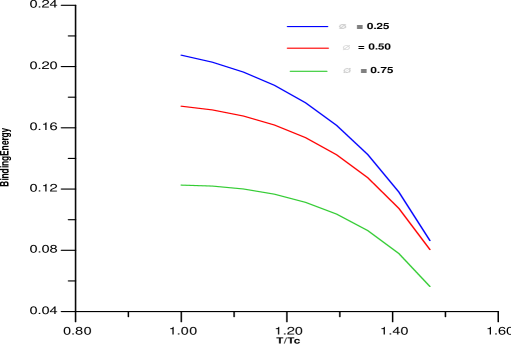
Figure 1: The binding energy is plotted as a function of $\frac{T}{T_{c}}$ for different values of $\Phi$ at u${}_{b}=0$ and $\alpha=1.0$

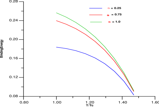
Figure 2: The binding energy is plotted as a function of $\frac{T}{T_{c}}$ for different values of $\Phi$ at u${}_{b}=0$ and $\alpha=0.25$

Figure 3: The binding energy is plotted as a function of $\frac{T}{T_{c}}$ for different values of $\alpha$ at u${}_{b}=0$ and $\Phi=0.25$

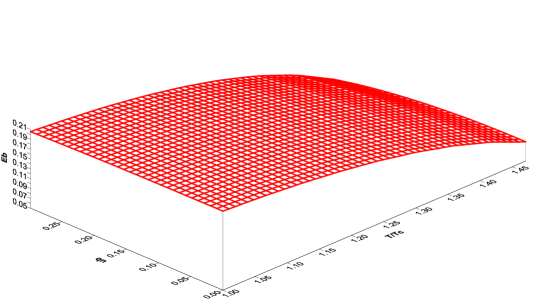
Figure 4: The binding energy is plotted as a function of u _b and $\frac{T}{T_{c}}$ at $\Phi=0.25$ and $\alpha=1$

Figure 5: The binding energy is plotted as a function of u _b and $\frac{T}{T_{c}}$ at $\Phi=0.25$ and $\alpha=0.4$

Figure 6: The binding energy is plotted as a function of u_b and $\frac{T}{T_{c}}$ at $\Phi=0.75$ and $\alpha=1$

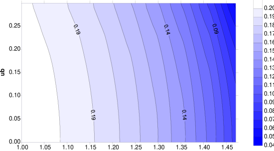
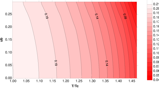
Figure 7: The binding energy is plotted as a contour of u_b and $\frac{T}{T_{c}}$ at $\Phi=0.25$ and $\alpha=0.4$

Figure 8: The binding energy is plotted as a contour of u_b and $\frac{T}{T_{c}}$ at $\Phi=0.75$ and $\alpha=1.0$

References

- [1] M. Abu-Shady and H. M. Mansour, Phys. Rev. C 85 (2012) 055204.
- [2] M. Abu-Shady, J. Egypt. Math. Soc. 25 (2017) 86.
- [3] M. Abu-Shady, Int. J. Mod. Phys. A 34 (2019) 1950201.
- [4] M. Abu-Shady, T. A. Abdel-Karim and Sh Y. Ezz-Alarab, J Egypt. Math. Soc. 27 (2019) 14.
- [5] M. Abu-Shady and A. N. Ikot, Eur. Phys. J Plus 134 (2019) 321.
- [6] M. Abu-Shady, H. M. Mansour and A. I. Ahmadov, Adv. High Energy Phys. 2019 (2019) 4785615.
- [7] M. Abu-Shady, T. A. Abdel-Karim and E. M. Khokha, Adv. High Energy Phys. 2018 (2018) 7356843.
- [8] M. Abu-Shady and H. M. Fath-Allah, Int. J Mod. Phys. A 35 (2020) 2050110.
- [9] M. Gell-Mann and M. Levy, Nuovo Cinmento 16, 705 (1960).
- [10] M. Birse and M. Banerjee, Phys. Rev. D 31, 118 (1985).
- [11] J. T. Lenaghan, D. H. Rischke and J. Schaffiner-Bielich, Phys. Rev. D 62, 085008 (2000).
- [12] D. Roder, J. Ruppert and D. H. Rischke, Phys. Rev. D 68, 016003 (2003).
- [13] M. Abu-Shady, Int. J Mod. Phys. E 21 (2012) 1250061.
- [14] M. Abu-Shady, Int. J. Theor. Phys. 49 (2010) 2425.
- [15] M. Abu-Shady, Int. J. Theor. Phys. 50 (2011) 1372.
- [16] M. Abu-Shady and M. Soleiman, Phys. Part. Nucl. Lett. 10 (2013) 683.
- [17] M. Abu-Shady, Mod. Phys. Lett. A 29 (2014) 1450176.
- [18] M. Abu-Shady and H. M. Mansour. J Phys. G: Nucl. Part. Phys. 43 (2015) 025001.
- [19] A. F. Nikiforov and V. B. Uvarov, Special Functions of Mathematical Physics, Birkhauser, Basel (1988).
- [20] F. Ahmed, Commun. Theor. Phys. 75, 055103 (2023).
- [21] F. Ahmed, Rev. Mex. Física 69, 030401 (2023).
- [22] F. Ahmed, Proc. Roy. Soc. A 479, 20220624 (2023).
- [23] F. Ahmed, EPL 141, 25003 (2023).
- [24] F. Ahmed, Phys. Scr. 98, 015403 (2023).
- [25] F. Ahmed, Indian J Phys 97, 2307 (2023).
- [26] F. Ahmed, Molecular Physics 120, e2124935 (2023).
- [27] F. Ahmed, Molecular Physics 121, e2155596 (2023).
- [28] F. Ahmed, Int. J Geom. Meth. Mod. Phys. 20, 2350060 (2023).
- [29] F. Ahmed, Molecular Physics 121, e2198617 (2023).
- [30] J. Fingberg, Phys. Lett. B 424, 343 (1998).
- [31] S. M. Kuchin and N. V. Maksimenko, Univ. J. Phys. Appl. 1, 295 (2013).
- [32] O. Kaczmarek, hep-let/07100498 (2007).
- [33] M. Moring, S. Ejir, O. Kaczmarek, F. Karsch and E. Laermann, PoSLAT 2005, 193 (2006).
- [34] B. Liu, P. N. Shen, and H. C. Chiang, Phys. Rev. C 55, 3021 (1997).