The cosmic variance of testing general relativity with gravitational-wave catalogs

Abstract

Combining multiple gravitational-wave observations allows for stringent tests of general relativity, targeting effects that would otherwise be undetectable using single-event analyses. We show that the finite size of the observed catalog induces a significant source of variance. If not appropriately accounted for, general relativity can be excluded with arbitrarily large credibility even if it is the underlying theory of gravity. This effect is generic and entirely analogous to the so-called “cosmic variance” of cosmology: in essence, we only have one catalog that contains all the events. We show that the cosmic variance holds for arbitrarily large catalogs and cannot be suppressed by selecting “golden” observations with large signal-to-noise ratios. We present a mitigation strategy based on bootstrapping (i.e. resampling with repetition) that allows assigning uncertainties to one’s credibility on the targeted test. We demonstrate our findings using both toy models and real gravitational-wave data. In particular, we quantify the impact of the cosmic variance on the ringdown properties of black holes using the latest LIGO/Virgo catalog.

Introduction— Gravitational-wave (GW) detections of binary compact objects allow for new tests of general relativity (GR) in the strong-field regime [1, 2] adding up to those performed with other experimental and astrophysical probes [3, 4]. Such tests are limited by the intrinsic challenges of modeling the strong-field dynamics in theories of gravity beyond GR [5, 6, 7, 8], which prevents a directed, model-dependent search [9]. In this regime, one primarily relies on testing the null hypothesis that GR is the underlying theory of gravity [10].

At the individual-event level, tests of GR have been performed since the very first GW detection of binary black holes (BHs) [2] and more stringent tests have since then been reported using the increasing number of detections during the first three LIGO/Virgo observing runs [11, 10, 12]. Combining multiple events, or stacking, is key to measure effects that are otherwise undetectable using single sources.

Existing approaches to stacking can be categorized as (i) multiplication of the individual likelihoods [13, 14], (ii) multiplication of the individual Bayes factors [15, 16, 17] and (iii) hierarchical inference [18, 19, 20]. Multiplication of the likelihoods assumes that deviations have the same values across all the events (e.g., constraints on the mass of the graviton) while multiplication of the Bayes factors assumes that deviations in multiple events are uncorrelated (e.g., constraints on additional BH hair) [18]. Both assumptions are unrealistic and Ref. [19] first proposed hierarchical stacking as a consistent way of combining observations, similarly to that of hierarchical Bayesian inference used in GW population studies [21, 22]. In this context, the consistency of the data with GR can be quantified by standard metrics such as credible levels and Bayes factors.

Care must be exercised when interpreting the results of tests of GR, as they can lead to incorrect conclusions in the presence of unmodeled physics (e.g., environmental effects [23, 24], eccentricity [25, 26]), systematics in the waveform templates [27, 28], stealth biases [29], and overlapping signals [30]. In fact, one could also revert the argument and use tests of GR as a complementary method to identify the presence of systematics [31].

In this letter, we investigate an additional source of uncertainty when performing catalog tests of GR, namely the variance originating from the finite size of the catalog itself. We show that, even if the null hypothesis is correct, it could be excluded with arbitrarily large credibility from the posterior of the deviation parameters when combining multiple events. The issue would be mitigated if one were to repeat the experiment multiple times, as large deviations would only occur in relatively few repetitions. However, by definition, we are only going to have one catalog that contains all the observations. In analogy with the known effect in cosmology [32, 33], we refer to the considerations above as the “cosmic variance” of strong-field gravity tests, meaning that we only observe one realization of all the possible catalogs of sources.

Crucially, our key message is that cosmic variance does not invalidate the use of null tests of GR, but it must be accounted for when interpreting the results. First, we show that using Bayes factors provides a more conservative evidence against violations of the null hypothesis than the corresponding credible intervals might suggest. Second, we design a mitigation strategy by assigning uncertainties to credible intervals and Bayes factors. Since one cannot use multiple realizations, we propose bootstrapping as a partial remedy [34]. In a nutshell, from the original dataset $\boldsymbol{d}=\{d_{1},\dots,d_{N}\}$ one resamples a new dataset with the same size $\boldsymbol{d}^{\rm boot}=\{d^{\rm boot}_{1},\dots,d^{\rm boot}_{N}\}$ allowing for repetitions. When resampling $\boldsymbol{d}$ with replacement, there are $\binom{2N-1}{N}$ distinct combinations and the probability of obtaining the original dataset is as small as $N!/N^{N}$ [35].

This mimics a set of repeated experiments to study the distribution of the chosen estimators (Bayes factors or credible intervals), which can then be used to extract summary statistics (e.g. standard deviation, interquantile range), thus providing uncertainty estimates.

We focus on hierarchical tests of GR as introduced in Ref. [19] as they represent the most general case. First, we perform numerical experiments to show that the cosmic variance holds for arbitrarily large catalogs and it cannot be mitigated by selecting the observations based on their signal-to-noise ratio (SNR). Then, we demonstrate the impact of the cosmic variance on real GW data by reproducing and extending a flagship test of GR. In particular, we consider the so-called pSEOBNR test [36] which targets deviations in the dominant frequency and damping time of the ringdown portion of the signal and was recently applied to the GWTC-3 catalog [12]. We show that, while the hierarchical analysis of the damping time appears to exclude GR with high credibility, the corresponding Bayes factor prefers GR and the bootstrapped distributions have significant support in favor of the null hypothesis.

Hierarchical stacking— We are interested in testing the null hypothesis (i.e. GR is the true theory) using a deviation parameter $x$, which is scaled such that it vanishes when the null hypothesis $\mathcal{H}_{0}$ is satisfied

$$\mathcal{H}_{0}:\mathcal{H}\wedge\{x=0\}\,,$$ (1)

where $\mathcal{H}$ is a broader hypothesis. If the null hypothesis $\mathcal{H}_{0}$ is inconsistent with the data, we expect deviations $x$ to spread away from $0$ following unknown patterns that are set by the system parameters and the nature of the deviations. We model the distribution of $x$ as a normal distribution $\mathcal{N}$ with mean $\mu$ and variance $\sigma^{2}$

$$p_{\rm pop}(x|\mu,\sigma^{2})=\mathcal{N}(x|\mu,\sigma^{2})\,.$$ (2)

In terms of these hyper-parameters, the null hypothesis maps to

$$\mathcal{H}_{0}:\mathcal{H}\wedge\{\mu=0,\sigma^{2}=0\}\,.$$ (3)

GR tests are performed by applying hierarchical population inference [21] to reconstruct the distribution of $\{\mu,\sigma^{2}\}$ from the observed events $\boldsymbol{d}=\{d_{1},\dots,d_{N}\}$. The posterior is given by

$$p(\mu,\sigma^{2}|\boldsymbol{d})\propto\mathcal{L}(\boldsymbol{d}|\mu,\sigma^{2})\pi(\mu,\sigma^{2})\,,$$ (4)

where the hierarchical likelihood

$$\mathcal{L}(\boldsymbol{d}|\mu,\sigma^{2})=\prod_{i=1}^{N}\int dx~{}\mathcal{L}(d_{i}|x)p_{\rm pop}(x|\mu,\sigma^{2})$$ (5)

can be expressed in terms of the likelihoods $\mathcal{L}(d_{i}|x)$ of the individual observations and $\pi(\mu,\sigma^{2})$ models the prior. Equation (5) assumes that the observations are independent of each other, which would be violated for, e.g., overlapping events. The expressions above do not include selection effects [21, 22] because in this context we do not wish to reconstruct the underlying distribution of $x$ but only constrain its value using the set of observed sources.

While one could consider more informative ansatzes in place of Eq. (2), Refs. [19, 20] showed that a Gaussian distribution can identify deviations from the null hypothesis even when these follow more complex patterns.

The consistency with the null hypothesis can be quantified using the quantile

$$Q_{0}=\int_{p\geq p(0,0)}p(\mu,\sigma^{2}|\boldsymbol{d})~{}d\mu d\sigma^{2}\,,$$ (6)

which is defined such that $Q_{0}=0$ ($Q_{0}=1$) indicate full consistency (full inconsistency).

The Bayes factor $\mathcal{B}$ in favor of the null hypothesis $\mathcal{H}_{0}$ over the broad hypothesis $\mathcal{H}$ can be estimated using the Savage-Dickey density ratio [37],

$$\mathcal{B}=\frac{p(\mu=0,\sigma^{2}=0|\mathbf{d})}{\pi(\mu=0,\sigma^{2}=0)}\equiv\frac{\mathcal{L}(\mathbf{d}|\mu=0,\sigma^{2}=0)}{\mathcal{Z}}$$ (7)

where $\mathcal{L}$ is the hyper-likelihood of Eq. (5) and $\mathcal{Z}=p(\mathbf{d})$ is the evidence of the data under $\mathcal{H}$. Bayes factors are often interpreted using Jeffreys’ scale [38], where $\mathcal{B}\geq 10^{2}$ ($\mathcal{B}\leq 10^{-2}$) denotes “decisive” evidence in favor of (against) the null hypothesis.

From Eq. (7), the Bayes factor scales as $\mathcal{B}\propto\Delta$, where $\Delta$ is the prior volume: wide priors favor the null hypothesis, vice-versa tight priors favor the alternative hypothesis. This implies one can artificially increase the odds for either of the two competing models by restricting or enlarging the prior volume [39]. In the following, we fix this ambiguity by restricting the original prior volume to the $(1-p)$ posterior credible interval along each axis. For concreteness, the fraction of discarded posterior samples is set to $p=1.973\times 10^{-9}$, which corresponds to a $6$-$\sigma$ interval if these were Gaussian distributions. We then rescale $\mathcal{B}$ by the ratio $\Delta_{\rm new}/\Delta_{\rm old}$ of the restricted and original prior volumes. The rationale behind our choice is that $\Delta_{\rm new}$ is just as large to encompass the vast majority of the posterior support and therefore, the resulting Bayes factor constitutes a somewhat conservative estimate when testing GR. We denote the resulting Bayes factor as $\mathcal{B}_{\star}$ to distinguish it from the prior-dependent expression reported in Eq. (7).

Cosmic variance— If the null hypothesis is correct, one would naively expect that the posterior for $\mu$ and $\sigma^{2}$ would become sharper around $\mu=\sigma^{2}=0$ as more events are added to the catalog; vice versa, it would peak away from zero if the null hypothesis is violated in nature.

It is straightforward to check this expectation using a toy model where $x$ has Gaussian likelihoods for all the events

$$\mathcal{L}(d_{i}|x)\propto\mathcal{N}(x|\mu_{{\rm obs},i},\sigma^{2}_{{\rm obs},i})$$ (8)

and errors are homoscedastic, i.e., $\sigma_{{\rm obs},i}=\sigma_{\rm obs}={\rm const.}$ In the limit of large catalogs $N\gg 1$, Eqs. (4) and (5) reduce to [20]

$$p(\mu,\sigma^{2}|\boldsymbol{d})\approx p(\mu|\boldsymbol{d})p(\sigma^{2}|\boldsymbol{d})\,,$$ (9)

with

$$p(\mu|\boldsymbol{d})\propto\mathcal{N}\left(\mu\left|{\rm mean}(\mu_{\rm obs}),\frac{{\rm var}(\mu_{\rm obs})}{N}\right.\right)$$ (10)

and

$$p(\sigma^{2}|\boldsymbol{d})\propto\mathcal{N}\left(\sigma^{2}\left|{\rm var}(\mu_{\rm obs})-\sigma_{\rm obs}^{2},\frac{2\,{\rm var}(\mu_{\rm obs})^{2}}{N}\right.\right)\,\!.$$ (11)

The true value of $x$ under the null hypothesis is $x_{\rm true}=0$, which implies the $\mu_{{\rm obs},i}$’s are independently sampled from a normal distribution

$$\mu_{{\rm obs},i}\sim\mathcal{N}(\mu_{{\rm obs},i}|\mu_{\rm true}=0,\sigma_{\rm obs}^{2})\,,$$ (12)

where the variance $\sigma_{\rm obs}^{2}$ accounts for the scatter due to noise in the detector consistently with the assumption of normal likelihoods [40]. The central limit theorem implies

$${\rm mean}(\mu_{\rm obs}) \sim\mathcal{N}\left({\rm mean}(\mu_{\rm obs})\left|0,\frac{\sigma_{\rm obs}^{2}}{N}\right.\right)\,,$$ (13)

$${\rm var}(\mu_{\rm obs}) \sim\mathcal{N}\left({\rm var}(\mu_{\rm obs})\left|\sigma_{\rm obs}^{2},\frac{2~{}\sigma_{\rm obs}^{2}}{N}\right.\right)\,.$$ (14)

Plugging Eq. (14) into Eq. (10) shows that the $\mu$ posterior has variance $\mathchar 21016\relax\,\sigma_{\rm obs}^{2}/N$ around ${\rm mean}(\mu_{\rm obs})$ at leading order in $N^{-1}$. By direct comparison with Eq. (13), it follows that $p(\mu|\boldsymbol{d})$ does not necessarily converge towards $\mu=0$ as $N$ increases, but there is a chance that the particular draw of $\{\mu_{{\rm obs},i}\}_{i=1}^{N}$ from (12) shifts its peak away from the true value $\mu_{\rm true}=\sigma^{2}_{\rm true}=0$. A similar conclusion applies to the recovery of $\sigma^{2}$ by direct comparison of Eq. (11) and (14). This toy model illustrates how the cosmic variance is due to the variance associated with the finite size $N$ of the catalog.

In writing Eqs. (10) and (11) we neglected the effects of the prior $\pi(\mu,\sigma^{2})$, i.e. we have assumed it is uniform and unbounded. However, the condition that $\sigma^{2}>0$ induces boundary effects in $p(\sigma^{2}|\boldsymbol{d})$. It follows that the posterior $p(\mu,\sigma^{2}|\boldsymbol{d})$ lacks a frequentist coverage of credible intervals, that is, it is not true that $Q_{0}>p$ in a fraction $(1-p)$ of similar experiments. The consequent difficulty of the statistical interpretation of $Q_{0}$ was already raised in Ref. [39].

We further highlight the impact of the cosmic variance by considering $1000$ catalogs of $N=10^{4}$ events each, with Gaussian likelihoods for $x$ as per Eq. (8) and three different choices for the stochastic uncertainties. First, (i) we consider the case of homoscedastic likelihoods with $\sigma_{\rm obs}=0.1$. Then, (ii) we assume heteroscedastic Gaussian likelihoods with $\sigma_{{\rm obs},i}=1/{\rm SNR}_{i}$, where ${\rm SNR}\in[10,1000]$ is a random variable distributed according to $p({\rm SNR})\propto{\rm SNR}^{-4}$ to mimic the density of SNRs expected from realistic GW detections [41]. Finally, (iii) we isolate from the same heteroscedastic catalogs only the events with ${\rm SNR}\geq 50$, which mimics a scenario where one performs tests of GR only on a loud subset of the available GW catalog. For each case, we draw the maximum-likelihood estimators $\mu_{{\rm obs},i}$ from $\mathcal{N}(\mu_{{\rm obs},i}|\mu_{\rm true}=0,\sigma_{{\rm obs},i}^{2})$ to capture noise scattering.

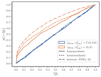
Figure 1: Cumulative distribution function of $Q_{0}$ for three sets of catalog realizations. We consider Gaussian likelihoods with homoscedastic errors (solid), heteroscedastic errors (dashed), and heteroscedastic with an SNR cut (dash-dotted). Orange and blue curves are produced by either assuming the null hypothesis $\mu_{\rm true}=0=\sigma_{\rm true}^{2}=0$ or drawing $(\mu_{\rm true},\sigma^{2}_{\rm true})$ from their prior, respectively.

We map the $(\mu,\sigma^{2})$ posterior distribution using the dynesty implementation of nested sampling [42] with 5000 live points and uniform priors $\mu\in[-0.9,0.9]$ and $\sigma^{2}\in[0,0.9]$. Figure 1 shows the resulting coverage of $Q_{0}$. To better highlight the peculiarity of the null hypothesis, we repeat the experiments without assuming that $\mu_{\rm true}=\sigma_{\rm true}^{2}=0$, but instead sample $(\mu_{\rm true},\sigma_{\rm true}^{2})$ from their uniform priors at each catalog realization. As expected, when catalogs are drawn from uniform priors in $(\mu_{\rm true},\sigma_{\rm true}^{2})$, the quantile $Q_{0}$ has a frequentist coverage. Instead, when drawing from the null hypothesis, the recovered values of $\sigma^{2}$ lie close to the edge of the prior, which produces an excess of low values of $Q_{0}$, thus pushing its cumulative distribution to the upper-right portion of Figure 1. That said, while $Q_{0}$ lacks a frequentist interpretation, it nonetheless provides an upper-bound estimate of the false alarm rate because $Q_{0}>p$ in less than a fraction $(1-p)$ of the catalog realizations. Figure 1 also shows that restricting to high-SNR events does not reduce the effect of cosmic variance, in agreement with our interpretation based on the finite size of the catalog.

Bootstrapping— The cosmic variance can be mitigated by assigning uncertainties to the chosen estimator. We showcase this idea by selecting a homoscedastic catalog realization with a high null-hypotesis quantile $Q_{0}=0.98$. The corresponding Bayes factor is $\log_{10}\mathcal{B}_{\star}=-0.65$, indicating substantial but not decisive evidence against the null hypothesis. After resampling for 1000 catalogs via bootstrap, we find that $Q_{0}>0.77$ and $\log_{10}\mathcal{B}_{\star}=-0.76^{+1.37}_{-2.61}$ at $90\%$ credibility. In particular, $\log_{10}\mathcal{B}_{\star}>0$ in $23\%$ of the bootstrapped catalogs, which is a non-negligible fraction and would suggest great care in claiming that the measurement provides evidence against the null hypothesis. This toy model shows that our proposed strategy is robust in mitigating false positives, even for catalogs with large credible quantiles.

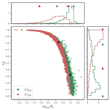
Figure 2: Distribution of Bayes factors $\log_{10}\mathcal{B}_{\star}$ and GR quantiles $Q_{0}$ over $1000$ bootstrapped realizations of the flagship pSEOBNR catalog test. Green crosses and red hexagons indicate constraints on the ringdown frequency $\delta\hat{f}_{220}$ and damping time $\delta\hat{\tau}_{220}$, respectively. In the marginalized histograms, colored triangles indicate 90% confidence intervals. Black markers indicate the values of $\log_{10}\mathcal{B}_{\star}$ and $Q_{0}$ corresponding to the original catalog; this is just one possible realization among many!

State-of-the-art application— We now apply our findings to a standard test of strong-field gravity with GWs. We consider the pSEOBNR family [43, 36, 31, 28] of binary BH waveforms, which are obtained by augmenting effective-one-body templates with free parameters corresponding to fractional deviations in the quasi-normal modes of the remnant BH. In the spirit of BH spectroscopy [44, 45], the pSEOBNR scheme has been used in tests of GR by allowing for deviations $\delta\hat{f}_{220}$ and $\delta\hat{\tau}_{220}$ in the dominant frequency and damping time respectively [10, 36, 12]. The latest iteration of these tests [12] uses 10 GW events and indicates a moderate deviation of $\delta\hat{\tau}_{220}$ from the GR value $\delta\hat{\tau}_{220}=0$. While insufficient to claim inconsistencies with GR, the authors themselves indicate this finding deserves further investigation.

In order to illustrate the role of the cosmic variance in the interpretation of the results, we reproduce the pSEOBNR analysis of Ref. [12] with a hierarchical stacking of the events. For consistency with Ref. [12], we recover the $(\mu,\sigma)$ posterior and set uniform priors $\mu\in[-0.9,0.9]$ and $\sigma\in[0,0.9]$, covering a region that is much broader than the resulting posterior. Quoting median and $90\%$ credibility, we obtain $\mu=0.02_{-0.04}^{+0.04}$, $\sigma<0.06$ for $\delta\hat{f}_{220}$ and $\mu=0.13^{+0.13}_{-0.11}$, $\sigma<0.19$ for $\delta\hat{\tau}_{220}$, which is in agreement with the analysis of Ref. [12]. Using Eq. (6), we quantify the consistency between GR and the data as $Q_{0}=0.32$ for $\delta\hat{f}_{220}$ and $Q_{0}=0.81$ for $\delta\hat{\tau}_{220}$. As already reported [12], the $\delta\hat{\tau}_{220}$ quantile indicates a moderate preference against the null hypothesis. Using Bayes factors, we find $\log_{10}\mathcal{B}_{\star}=1.49$ for $\delta\hat{f}_{220}$ and $\log_{10}\mathcal{B}_{\star}=0.70$ for $\delta\hat{\tau}_{220}$. In particular, we note that in the case of $\delta\hat{\tau}_{220}$, even if $Q_{0}=0.81$, the Bayes factor favors the null hypothesis.

We assign uncertainties to $Q_{0}$ and $\log_{10}\mathcal{B}_{\star}$ by generating 1000 bootstrapped catalog realizations. For each of these, we repeat the hierarchical analysis and extract the corresponding values of $Q_{0}$ and $\mathcal{B}_{\star}$. The analysis of Ref. [12] uses 10 GW events, which implies there are $\mathchar 21016\relax\,10^{5}\gg 1000$ [35] independent realizations and the probability of duplications is consequently small. Our results are shown in Figure 2. For $\delta\hat{f}_{220}$ we find that $\log_{10}\mathcal{B}_{\star}=1.45_{-0.83}^{+0.25}$ and $Q_{0}<0.77$ at 90% confidence. For $\delta\hat{\tau}_{220}$, we find $\log_{10}\mathcal{B}_{\star}=0.62_{-1.19}^{+0.70}$ and $Q_{0}>0.42$.

Our bootstrap procedure returns broad histograms for $Q_{0}$; in particular, the credible quantile of the null hypothesis for $\delta\hat{\tau}_{220}$ can be as low as $Q_{0}=0.42$ within the $90\%$ range. Accounting for the cosmic variance mitigates the significance of the inference performed with the original observed catalog. Moreover, the distribution of the Bayes factors for $\delta\hat{\tau}_{220}$ does not signal any substantial evidence against the null hypothesis at $90\%$ credibility; rather, $83\%$ of the samples have $\log_{10}\mathcal{B}_{\star}>0$, indicating support for the null hypothesis.

Finally, the correlation between $Q_{0}$ and $\log_{10}\mathcal{B}_{\star}$ shown Figure 2 indicates that Bayes factors provide weaker evidence against the null hypothesis than the corresponding credible level. In particular, while there are individual catalog realizations with $Q_{0}\approx 1$, the corresponding Bayes factors barely meet the threshold for decisive evidence.

Discussion— Combining information from multiple observations is a natural strategy to strengthen one’s statistical inference on a physical phenomenon. Testing gravity with GWs is no exception. GR is a fundamental pillar of our understanding of the Universe and, when the stakes are so high, our confidence in experimental bounds becomes critical. The interpretation of tests of GR with GW catalogs depends on both the statistics (e.g. quantiles and Bayes factors) as well as the techniques (e.g. hierarchical stacking) used to combine the inferences in favor or against the null hypothesis. Crucially, one must also quantify the cosmic variance originating from the single realization of the catalog of GW events at our disposal.

In particular, three key points are worth stressing:

• The net effect of the cosmic variance is to soften one’s claim in favor of violations of GR. After all, the GW catalog we happened to observe might be an unlucky realization of the null hypothesis.

• The cosmic variance can be quantified by producing multiple mock catalogs. We propose a data-driven approach that does not rely on assuming a population of sources but instead resamples the observed catalog with repetition.

• The cosmic variance does not vanish as either the size of the catalog or the SNR of the events increase.

Points (i) and (ii) are best exemplified on the BH ringdown test we borrowed from the flagship analysis of Ref. [12]. We show that, while the current catalog presents a quantile $Q_{0}$ that might be interpreted as a moderate deviation from GR, this evidence turns out to be insignificant when the original measurement is considered as a part of a distribution of bootstrapped estimators. We have illustrated point (iii) with a toy model based on Gaussian likelihoods.

Our findings lead to the conceptual issue of whether one should test the null hypothesis using Bayesian model selection in the context of tests of GR. As pointed out in Ref. [39], reporting the evidence against GR with Bayesian estimators using free deviation parameters is questionable: results are prior-dependent and not reparametrization-invariant, while credible intervals lack a frequentist interpretation. On the other hand, a frequentist approach based on the $p$-value only assesses the likelihood of the experimental outcome given the null hypothesis and can be considered more resilient. Unfortunately, implementing a pure $p$-value test in this context is, in practice, unfeasible because one would need to know the true population distribution of the events.

Bootstrapping is a possible way out but only provides a partial solution. Bootstrap samples inevitably inherit the peculiarities (e.g. outliers) of the specific catalog realization we have observed. We speculate another promising avenue in this direction is to incorporate population inference into tests of GR [46] while relying on the notion of “Bayesian $p$-values” [47]. A safer solution is to settle for weaker but more confident statements. This can be done trivially by breaking down the catalogs into chunks, using fewer events to compute the chosen estimator but obtaining multiple estimates.

While we concentrated on tests of GR, the cosmic variance is a generic effect, both within and outside of GW astronomy (e.g. Ref. [48]). For instance, astrophysical inferences from GW observations of binary populations [49] and cosmological models [50] are impacted by the cosmic variance in much the same fashion. The considerations put forward in this work are relevant to assess the statistical significance of some of those findings, especially when the significance itself is deemed to be weak.

Acknowledgments— We thank Andrea Maselli, Riccardo Buscicchio, and Golam Shaifullah for discussions. C.P. and D.G. are supported by ERC Starting Grant No. 945155–GWmining, Cariplo Foundation Grant No. 2021-0555, MUR PRIN Grant No. 2022-Z9X4XS, and the ICSC National Research Centre funded by NextGenerationEU. D.G. is supported by MSCA Fellowship No. 101064542–StochRewind and Leverhulme Trust Grant No. RPG-2019-350. S.B. is supported by UKRI Stephen Hawking Fellowship No. EP/W005727. Computational work was performed at CINECA with allocations through INFN and Bicocca.

References

- Baker et al. [2015] T. Baker, D. Psaltis, and C. Skordis, Astrophys. J. 802, 63 (2015), arXiv:1412.3455 [astro-ph.CO] .
- Abbott et al. [2016] B. P. Abbott et al., Phys. Rev. Lett. 116, 221101 (2016), [Erratum: Phys.Rev.Lett. 121, 129902 (2018)], arXiv:1602.03841 [gr-qc] .
- Berti et al. [2015] E. Berti et al., Class. Quant. Grav. 32, 243001 (2015), arXiv:1501.07274 [gr-qc] .
- Will [2014] C. M. Will, Living Rev. Rel. 17, 4 (2014), arXiv:1403.7377 [gr-qc] .
- Witek et al. [2019] H. Witek, L. Gualtieri, P. Pani, and T. P. Sotiriou, Phys. Rev. D 99, 064035 (2019), arXiv:1810.05177 [gr-qc] .
- Okounkova et al. [2020] M. Okounkova, L. C. Stein, J. Moxon, M. A. Scheel, and S. A. Teukolsky, Phys. Rev. D 101, 104016 (2020), arXiv:1911.02588 [gr-qc] .
- Okounkova [2020] M. Okounkova, Phys. Rev. D 102, 084046 (2020), arXiv:2001.03571 [gr-qc] .
- East and Ripley [2021] W. E. East and J. L. Ripley, Phys. Rev. D 103, 044040 (2021), arXiv:2011.03547 [gr-qc] .
- Yunes et al. [2016] N. Yunes, K. Yagi, and F. Pretorius, Phys. Rev. D 94, 084002 (2016), arXiv:1603.08955 [gr-qc] .
- Abbott et al. [2021a] R. Abbott et al., Phys. Rev. D 103, 122002 (2021a), arXiv:2010.14529 [gr-qc] .
- Abbott et al. [2019] B. P. Abbott et al., Phys. Rev. D 100, 104036 (2019), arXiv:1903.04467 [gr-qc] .
- Abbott et al. [2021b] R. Abbott et al., (2021b), arXiv:2112.06861 [gr-qc] .
- Del Pozzo et al. [2011] W. Del Pozzo, J. Veitch, and A. Vecchio, Phys. Rev. D 83, 082002 (2011), arXiv:1101.1391 [gr-qc] .
- Ghosh et al. [2016] A. Ghosh et al., Phys. Rev. D 94, 021101 (2016), arXiv:1602.02453 [gr-qc] .
- Gossan et al. [2012] S. Gossan, J. Veitch, and B. S. Sathyaprakash, Phys. Rev. D 85, 124056 (2012), arXiv:1111.5819 [gr-qc] .
- Agathos et al. [2014] M. Agathos, W. Del Pozzo, T. G. F. Li, C. Van Den Broeck, J. Veitch, and S. Vitale, Phys. Rev. D 89, 082001 (2014), arXiv:1311.0420 [gr-qc] .
- Meidam et al. [2014] J. Meidam, M. Agathos, C. Van Den Broeck, J. Veitch, and B. S. Sathyaprakash, Phys. Rev. D 90, 064009 (2014), arXiv:1406.3201 [gr-qc] .
- Zimmerman et al. [2019] A. Zimmerman, C.-J. Haster, and K. Chatziioannou, Phys. Rev. D 99, 124044 (2019), arXiv:1903.11008 [astro-ph.IM] .
- Isi et al. [2019] M. Isi, K. Chatziioannou, and W. M. Farr, Phys. Rev. Lett. 123, 121101 (2019), arXiv:1904.08011 [gr-qc] .
- Isi et al. [2022] M. Isi, W. M. Farr, and K. Chatziioannou, Phys. Rev. D 106, 024048 (2022), arXiv:2204.10742 [gr-qc] .
- Mandel et al. [2019] I. Mandel, W. M. Farr, and J. R. Gair, Mon. Not. Roy. Astron. Soc. 486, 1086 (2019), arXiv:1809.02063 [physics.data-an] .
- Vitale et al. [2020] S. Vitale, D. Gerosa, W. M. Farr, and S. R. Taylor, in Handbook of Gravitational Wave Astronomy (Springer, 2020) arXiv:2007.05579 [astro-ph.IM] .
- Barausse et al. [2014] E. Barausse, V. Cardoso, and P. Pani, Phys. Rev. D 89, 104059 (2014), arXiv:1404.7149 [gr-qc] .
- Berti et al. [2022] E. Berti, V. Cardoso, M. H.-Y. Cheung, F. Di Filippo, F. Duque, P. Martens, and S. Mukohyama, Phys. Rev. D 106, 084011 (2022), arXiv:2205.08547 [gr-qc] .
- Saini et al. [2022] P. Saini, M. Favata, and K. G. Arun, Phys. Rev. D 106, 084031 (2022), arXiv:2203.04634 [gr-qc] .
- Bhat et al. [2023] S. A. Bhat, P. Saini, M. Favata, and K. G. Arun, Phys. Rev. D 107, 024009 (2023), arXiv:2207.13761 [gr-qc] .
- Moore et al. [2021] C. J. Moore, E. Finch, R. Buscicchio, and D. Gerosa, iScience 24, 102577 (2021), arXiv:2103.16486 [gr-qc] .
- Toubiana et al. [2023] A. Toubiana, L. Pompili, A. Buonanno, J. R. Gair, and M. L. Katz, (2023), arXiv:2307.15086 [gr-qc] .
- Vallisneri and Yunes [2013] M. Vallisneri and N. Yunes, Phys. Rev. D 87, 102002 (2013), arXiv:1301.2627 [gr-qc] .
- Hu and Veitch [2023] Q. Hu and J. Veitch, Astrophys. J. 945, 103 (2023), arXiv:2210.04769 [gr-qc] .
- Maggio et al. [2023] E. Maggio, H. O. Silva, A. Buonanno, and A. Ghosh, Phys. Rev. D 108, 024043 (2023), arXiv:2212.09655 [gr-qc] .
- Kamionkowski and Loeb [1997] M. Kamionkowski and A. Loeb, Phys. Rev. D 56, 4511 (1997), arXiv:astro-ph/9703118 .
- Portsmouth [2004] J. Portsmouth, Phys. Rev. D 70, 063504 (2004), arXiv:astro-ph/0402173 .
- Ivezić et al. [2020] Ž. Ivezić, A. J. Connolly, J. T. VanderPlas, and A. Gray, Statistics, Data Mining, and Machine Learning in Astronomy (Princeton, 2020).
- [35] N. J. Sloane et al., The On-Line Encyclopedia of Integer Sequences Sequence A001700, https://oeis.org/A001700.
- Ghosh et al. [2021] A. Ghosh, R. Brito, and A. Buonanno, Phys. Rev. D 103, 124041 (2021), arXiv:2104.01906 [gr-qc] .
- Dickey [1971] J. M. Dickey, The Annals of Mathematical Statistics 42, 204 (1971).
- Jeffreys [1998] H. Jeffreys, The Theory of Probability (Oxford, 1998).
- Chua and Vallisneri [2020] A. J. K. Chua and M. Vallisneri, (2020), arXiv:2006.08918 [gr-qc] .
- Vallisneri [2008] M. Vallisneri, Phys. Rev. D 77, 042001 (2008), arXiv:gr-qc/0703086 .
- Schutz [2011] B. F. Schutz, Class. Quant. Grav. 28, 125023 (2011), arXiv:1102.5421 [astro-ph.IM] .
- Speagle [2020] J. S. Speagle, Mon. Not. Roy. Astron. Soc. 493, 3132 (2020), arXiv:1904.02180 [astro-ph.IM] .
- Brito et al. [2018] R. Brito, A. Buonanno, and V. Raymond, Phys. Rev. D 98, 084038 (2018), arXiv:1805.00293 [gr-qc] .
- Dreyer et al. [2004] O. Dreyer, B. J. Kelly, B. Krishnan, L. S. Finn, D. Garrison, and R. Lopez-Aleman, Class. Quant. Grav. 21, 787 (2004), arXiv:gr-qc/0309007 .
- Berti et al. [2006] E. Berti, V. Cardoso, and C. M. Will, Phys. Rev. D 73, 064030 (2006), arXiv:gr-qc/0512160 .
- Payne et al. [2023] E. Payne, M. Isi, K. Chatziioannou, and W. M. Farr, (2023), arXiv:2309.04528 [gr-qc] .
- Vallisneri et al. [2023] M. Vallisneri, P. M. Meyers, K. Chatziioannou, and A. J. K. Chua, (2023), arXiv:2306.05558 [astro-ph.HE] .
- Roebber et al. [2016] E. Roebber, G. Holder, D. E. Holz, and M. Warren, Astrophys. J. 819, 163 (2016), arXiv:1508.07336 [astro-ph.CO] .
- Abbott et al. [2023a] R. Abbott et al., Phys. Rev. X 13, 011048 (2023a), arXiv:2111.03634 [astro-ph.HE] .
- Abbott et al. [2023b] R. Abbott et al., Astrophys. J. 949, 76 (2023b), arXiv:2111.03604 [astro-ph.CO] .