Fishnets: Information-Optimal, Scalable Aggregation for Sets and Graphs

Abstract

Set-based learning is an essential component of modern deep learning and network science. Graph Neural Networks (GNNs) and their edge-free counterparts Deepsets have proven remarkably useful on ragged and topologically challenging datasets. The key to learning informative embeddings for set members is a specified aggregation function, usually a sum, max, or mean. We propose Fishnets, an aggregation strategy for learning information-optimal embeddings for sets of data for both Bayesian inference and graph aggregation. We demonstrate that i) Fishnets neural summaries can be scaled optimally to an arbitrary number of data objects, ii) Fishnets aggregations are robust to changes in data distribution, unlike standard deepsets, iii) Fishnets saturate Bayesian information content and extend to regimes where MCMC techniques fail and iv) Fishnets can be used as a drop-in aggregation scheme within GNNs. We show that by adopting a Fishnets aggregation scheme for message passing, GNNs can achieve state-of-the-art performance versus architecture size on ogbn-protein data over existing benchmarks with a fraction of learnable parameters and faster training time.

1 Introduction

Aggregating information from independent data in an optimal way is a fundamental problem in statistics and machine learning. On one hand, frequentist analyses need optimal estimators for data compression, while on the other Bayesian analyses need small informative summaries for simulation-based inference (SBI) schemes (Cranmer et al., 2020). In a deep learning context graph neural networks (GNNs) rely on aggregation schemes to pool information over large data structures, where each feature might be weakly informative, but at a graph level might contribute a lot of information for predictive or regression tasks (Zhou et al., 2020).

Up until now, graph aggregation schemes have relied on simple, fixed operations such as mean, max, sum, (Kipf & Welling, 2017; Hamilton et al., 2017; Xu et al., 2019), variance, or trainable variants of these aggregators (Battaglia et al., 2018; Li et al., 2020). We introduce a new optimal aggregation scheme grounded in information-theoretic principles. By leveraging the additive structure of the log-likelihood for independent data and underlying Fisher curvature, we can construct a learned summary space that asymptotically contains maximal information (Vaart, 1998; Coulton & Wandelt, 2023). We show that this formalism captures relevant information in both a Bayesian inference context as well as for edge aggregation in graphs.

Our approach boasts several advantages. By explicitly learning the score and corresponding inverse-Fisher weights, we are able to construct aggregated summaries that are both asymptotically optimal and robust to changes in data distribution. The result is that we are able to construct optimal summary statistics for independent data for SBI applications, and using the same formalism are able to beat key benchmark GNN learning tasks with far smaller architectures in faster training time than leading networks.

This paper is organised as follows: We first present the Fishnets neural embedding method and review relevant related work in common notation. Next we demonstrate information saturation, robustness, and scalability in a Bayesian context for increasingly difficult problems, and highlight where existing aggregators fall short. Finally, we show that adopting Fishnets aggregation as a drop-in replacement for existing GNN architectures allows networks to outperform standard benchmark architectures with fewer learnable parameters and faster training time.

2 Method: Optimal Aggregation of Independent (Heterogeneous) Data

Maximum likelihood estimators (MLEs) are the asymptotically-optimal estimators for predictive tasks. When they are available, they provide an optimally-informative embedding of the data with respect to the parameters of interest, $\bm{\theta}$ (Alsing & Wandelt, 2018).

Many inference problems consist of a set of $n_{\rm data}$ data vectors, $\{\textbf{d}_{i}\}_{i=1}^{n_{\rm data}}$ which obey a global model controlled by parameters $\bm{\theta}$, and a possibly arbitrarily deep hierarchy of latent values, $\eta$. The full data likelihood for interesting parameters $\bm{\theta}$ is given by the integral over latents,

$$p(\{\textbf{d}_{i}\}|\bm{\theta})=\int p(\{\textbf{d}_{i}\}|\bm{\theta},\eta)p(\eta|\bm{\theta})d\eta.$$ (1)

When the data are independently distributed, their log-likelihood takes the form

$$\ln p(\{\textbf{d}_{i}\}|\bm{\theta})=\sum_{i=1}^{n_{\rm data}}\ln p(\textbf{d}_{i}|\bm{\theta}).$$ (2)

A maximum likelihood estimator can then be formed (iteratively) by the Fisher scoring method (Alsing & Wandelt, 2018):

$$\hat{\bm{\theta}}^{\rm MLE}=\bm{\theta}_{\rm fid}+\textbf{F}^{-1}\textbf{t},$$ (3)

which requires knowledge of the score, t, and Fisher matrix, F. For problems like linear regression where the analytic form of F and t are known, Eq. (3) gives the exact MLE for the parameters in a single iteration in the Gaussian approximation, given the dataset. In the case of independent data, both of the score and Fisher information are additive.

Taking the gradient of the log-likelihood with respect to the parameters, the score $\textbf{t}=\bm{\nabla}_{\bm{\theta}}\ln p(\{\textbf{d}_{i}\}|\bm{\theta})$ for the full dataset is the sum of the scores of the individual data points:

$$\textbf{t}=\sum_{i=1}^{n_{\rm data}}\bm{\nabla}_{\bm{\theta}}\ln p(\textbf{d}_{i}|\bm{\theta})=\sum_{i=1}^{n_{\rm data}}\textbf{t}_{i}(\textbf{d}_{i})$$ (4)

Taking the gradient again yields the Hessian, or Fisher information matrix (Amari, 2021; Vaart, 1998) for the dataset,

$$\textbf{F}=\sum_{i=1}^{n_{\rm data}}\bm{\nabla}_{\bm{\theta}}\bm{\nabla}_{\bm{\theta}}^{T}\ln p(\textbf{d}_{i}|\bm{\theta})=\sum_{i=1}^{n_{\rm data}}\textbf{F}_{i}(\textbf{d}_{i}),$$ (5)

which is also comprised of a sum of Fisher matrices of individual data. Once the score and Fisher matrix for a dataset are known, the two can be combined to form a pseudo-maximum likelihood estimate (MLE) for the target parameters following Equation (3). Therefore, constructing optimal embeddings of independent data with respect to specific quantities of interest just requires aggregating the scores and Fishers, and combining them as in Eq. 3. However, in general explicit forms for the likelihood (per data vector) may not be known. In this general case, as we will show in the following section, we can parameterize and learn the score and Fisher information using neural networks.

2.1 Twin Fisher-Score Networks

For many problems, however, the exact form of the Fisher and score are not known. Here we propose learning these functions with neural networks. Due to the additive structure of Eqs (5) and (4), we can parameterize the per-datapoint score and Fisher with twin neural networks:

$$\hat{\textbf{t}}_{i} =\textbf{t}(\textbf{d}_{i},\bm{\sigma}_{i};w_{t});\ \ \ \ \textbf{t}_{\rm NN}=\sum_{i}^{n_{\rm data}}\hat{\textbf{t}}_{i}$$ (6)

$$\hat{\textbf{F}}_{i} =\textbf{F}(\textbf{d}_{i},\bm{\sigma}_{i};w_{F});\ \ \ \ {\textbf{F}}_{\rm NN}=\sum_{i}^{n_{\rm data}}\hat{\textbf{F}}_{i}$$ (7)

where the score and Fisher network are parameterized by weights $w_{t}$ and $w_{F}$, respectively. The twin networks output a score and Fisher for each datapoint (see Appendix A for formalism), which are then each summed to obtain a global score and Fisher for the dataset. We can then compute parameter estimates using these aggregated embeddings following Eq. 3:

$$\hat{\bm{\theta}}_{\rm NN}=\bm{\theta}_{\rm fid}+\textbf{F}^{-1}_{\rm NN}\textbf{t}_{\rm NN}$$ (8)

Provided the embeddings $\hat{\textbf{t}}_{i}$ and $\hat{\textbf{F}}_{i}$ are learned sufficiently well, the summation formalism can be used to obtain Fisher and score estimates for datasets with heterogeneous structure and arbitrary size. These summaries can be regarded as sufficient statistics, since the score as a function of parameters could in principle be used to reconstruct the likelihood surface up to a constant (Alsing & Wandelt, 2018; Hoffmann & Onnela, 2022).

Loss Function. The twin networks can then be trained jointly using a negative-log Gaussian loss:

$$\mathcal{L}=\frac{1}{2}(\bm{\theta}-\hat{\bm{\theta}}_{\rm NN})^{T}\textbf{F}_{\rm NN}(\bm{\theta}-\hat{\bm{\theta}}_{\rm NN})-\frac{1}{2}\ln\det\textbf{F}_{\rm NN}.$$ (9)

Minimizing this loss ensures that information is saturated via maximising the aggregated Fisher, and forces the distance between embedding MLE and parameters to be minimized with respect to the Cramér-Rao bound (Cramér, 1946) as a function of parameters. This loss can also be interpreted as a maximum likelihood (MLE) loss for the parameters of interest $\theta$, as opposed to typical mean-square error (MSE) regression losses (see Appendix C for deepsets formalism details).

3 Related Work

Deepsets Mean Aggregation. A comparable method for learning over sets of data is regression using the Deepsets (DS) formalism (Zaheer et al., 2018). Here an embedding $f(\textbf{d}_{i};w_{1})$ is learned for each datum, and then aggregated with a fixed permutation-invariant scheme and fed to a global function $g$:

$$\hat{\bm{\theta}}=g\left(\bigoplus_{i=1}^{n_{\rm data}}f(\textbf{d}_{i};w_{1});\ \ w_{2}\right),$$ (10)

The networks are optimised minimising a squared loss against the true parameters, $\rm{MSE}(\hat{\bm{\theta}},\bm{\theta})$. When the aggregation is chosen to be the mean, the deepsets formalism is scalable to arbitrary data and becomes equivalent to the Fishnets aggregation formalism with flat weights across the aggregated data (see Appendix C for in-depth treatment).

Learned Softmax Aggregation. Li et al. present a learnable softmax counterpart to the DS aggregation scheme in the context of edge aggregation in GNNs. Using the above notation, their aggregation scheme reads:

$$\text{SoftmaxAgg}(\cdot)=\sum_{i=1}^{n_{\rm data}}\frac{\exp{\left(\beta\textbf{d}_{i}\right)}}{\sum_{l}\exp{\left(\beta\textbf{d}_{l}\right)}}\cdot\textbf{d}_{i}$$ (11)

where $\beta$ is a learned scalar temperature parameter. They show that adopting this aggregation scheme allows more graph convolution (GCN) layers to be stacked efficiently to deepen GNN models. Many other aggregation frameworks have been studied, including Graph Attention (Veličković et al., 2018), LSTM units (Hamilton et al., 2017), and scaled multiple aggregators (Corso et al., 2020).

4 Experiments: Bayesian Information Saturation

Bayesian Simulation Based Inference (SBI) provides a framework in which to perform inference with intractable likelihood. There have been massive developments in SBI, such as neural ratio estimation (Miller et al., 2021) and density estimation (Alsing et al., 2019; Papamakarios et al., 2019). Key to all of these methods is compressing a large number of data down to small summaries–typically one informative summary per parameter of interest to preserve information (Alsing & Wandelt, 2018; Charnock et al., 2018; Makinen et al., 2021). ML methods like regression (Jeffrey & Wandelt, 2020) and information-maximising neural networks (Charnock et al., 2018; Makinen et al., 2022, 2021) are very good at learning embeddings for highly structured data like images, and can do so losslessly (Makinen et al., 2021). For unstructured datasets comprised of many independent data, the task of constructing optimal summaries amounts to an aggregation task (Zaheer et al., 2018; Hoffmann & Onnela, 2022; Wagstaff et al., 2019). The Fishnets formalism is an optimal version of this aggregation. What deepsets and “learned” aggregation functions are missing is explicitly constructing the inverse-Fisher weights per datapoint, as well as being able to construct the total Fisher information, which is required to turn summaries into unbiased estimators (Alsing & Wandelt, 2018). Explicitly learning the $\textbf{F}^{-1}$ weights in addition to the score allows us to achieve 1) asymptotic optimality 2) scalability, and 3) robustness to changes in information content among the data.

In this section we demonstrate the 1) information saturation, 2) robustness and 3) scalability of the Fishnets aggregation through two examples in the context of SBI, and highlight the shortcomings of existing aggregators.

We first investigate a linear regression scaling problem and introduce a robustness test in which Fishnets outperforms deepset and learned softmax aggregation on test data. We then extend Fishnets to an inference problem with nuisance (latent) parameters and censorship to demonstrate the applicability of network scaling to a regime where MCMC becomes intractable.

4.1 Validation Case: Linear Regression

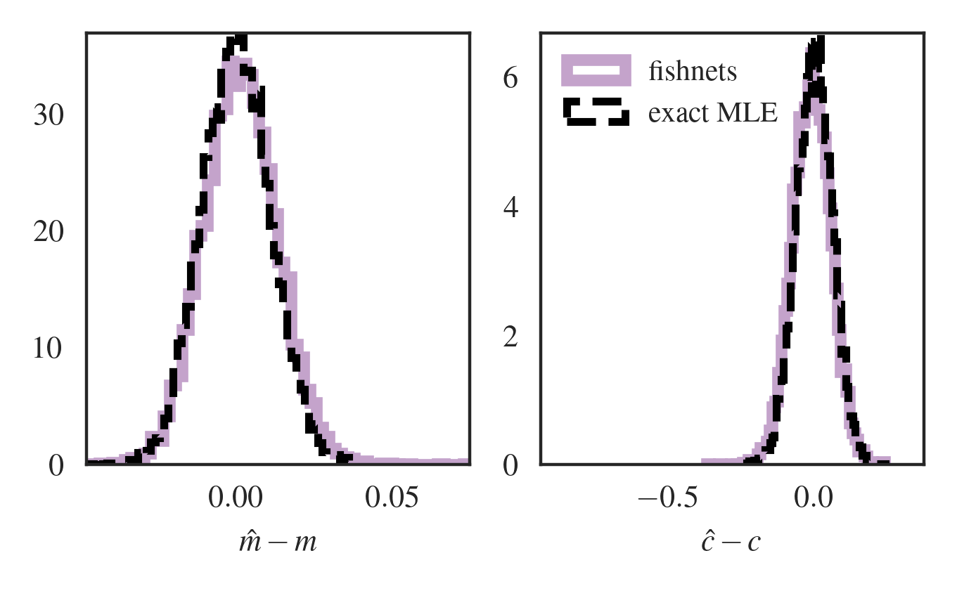
Figure 1: Fishnets saturate information for datasets 20 times larger than the training set. Residual maximum likelihood estimates for slope (left) and intercept (right) scatter about the truth for linear regression test datasets of size $n_{\rm data}=10^{4}$. The solid pink line is obtained from a weighted average of an ensemble of Fishnets networks, which were trained on datasets of size $n_{\rm data}=500$.

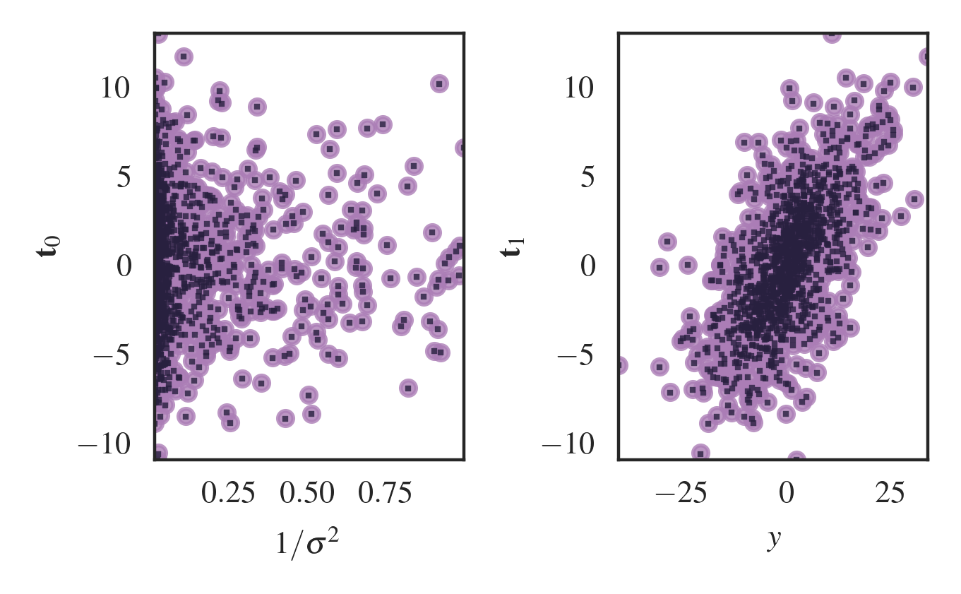
Figure 2: Fishnets achieve the exact form of the score as a function of input data in the linear regression case, indicating information saturation. Slices of true (dark) and network predicted (pink) score vector components as a function of data inputs for the $n_{\rm data}=10^{4}$ test set.

We use a toy linear regression model to validate our method and demonstrate network scalability. We consider the form $y=mx+b+\epsilon$, where $\epsilon\sim\mathcal{N}(0,\sigma)$, where the parameters of interest are the slope and intercept $\bm{\theta}=(m,b)$. This likelihood has an analytically-calculable score and Fisher matrix (see Appendix B.1), which can be used to calculate exact MLE estimates for the parameters $\bm{\theta}=(m,b)$ via Eq. (3). We choose wide Gaussian priors for $\theta$, and uniform distributions for $x\in[0,10]$ and $\sigma\in[1,10]$. For network training, we simulate $10^{4}$ datasets of size $n_{\rm data}=500$ datapoints. We use fully-connected MLPs of size [256, 256, 256] with ELU activations (Clevert et al., 2015) for both score and Fisher networks. Both networks receive the input data $[y_{i},x_{i},\sigma_{i}^{2}]^{T}$. We train networks for 2500 epochs with an adam optimizer using a step learning rate decay schedule. We train an ensemble of 10 networks in parallel on the same training data with different initializations. For testing, we generate an additional $10^{4}$ datasets of size $n_{\rm data}=10^{4}$ datapoints to demonstrate scalability.

Results. We display a comparison of test set performance to the true MLE solution in Figure 1, and slices of the true and predicted score vectors as a function of input data. The networks are able to recover the exact score and Fisher information matrices (see Figure 2), even when scaled up 20-fold. This test demonstrates that Fishnets can (1) saturate information on small training sets to enable scalable predictions on far larger aggregations of data (2).

4.2 Robustness to Changes in the Underlying Data Distributions

In real-world applications, actual data processed by a network might follow a different distribution than that seen in training. Here we compare three different network formalisms on changing shapes of target data distributions.

We train three networks on the same $n_{\rm data}=500$ datasets as before: a sum-aggregated Fishnets network, a mean-aggregated deepset, and a learned softmax-aggregated deepset (no Fisher output and standard MSE loss against true parameters $\rm{MSE}(\hat{\bm{\theta}},\bm{\theta})$). Here we initialise Fishnets with [50,50,50] hidden units for score and Fisher networks, and two embeddings of [128,128,128] hidden units for both deepset networks, all with swish (Ramachandran et al., 2017) nonlinearities for the data embedding (see Table 1). All networks are initialised with the same seed (see Appendix B.2 for architecture details).

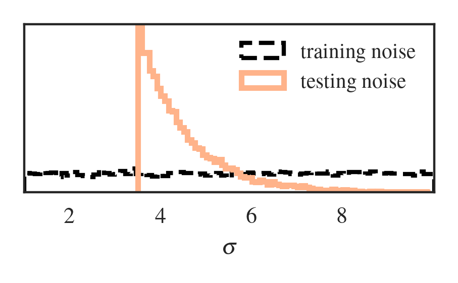
(a) Changing noise distribution.

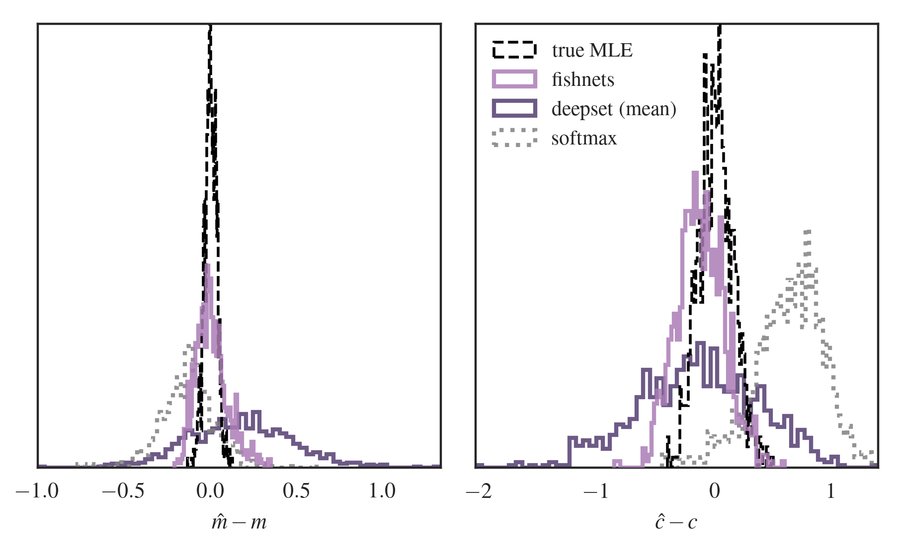
(b) Robustness testing different aggregators

Figure 3: Fishnets (pink, 3(b)) are robust to different noise distributions in test data, shown in 3(a). 3(b): Deepsets (grey) can return biased results for some parameters (left) and lossy estimates for others (right). Learned softmax aggregation appears to provide lossier and biased parameter estimates.

We apply our trained networks to test data $n_{\rm data}=850$ with noise variances and $x$ values drawn from different distributions to the training data: $\sigma\curvearrowleft\textrm{Exp}(\lambda=1.0)$ centred at $\sigma=3.5$, truncated at $\sigma=10.0$, and $x\curvearrowleft\mathcal{U}(0,3)$. The noise and covariate distributions have the same support as the training data, but have different expectation values and distributions, which can pose a problem for the mean-aggregation used in the standard deepsets formalism. We display results in Figure 3.

The heterogeneous Fishnets aggregation allows the network to correctly embed the noisy data drawn from the different distributions, while a significant loss in information can be seen for flat mean aggregation. The learned softmax aggregation improves the width of the residual distribution, but is still significantly wider than the Fishnets solution. We quote numeric results in Table 1.

These robustness tests show that Fishnets successfully learns per-object embeddings (score) and weights (Fisher) within sets, while being robust to changing shapes of the training distributions of these quantities (3). This test also shows that even in a very simple prediction scenario, common and learned aggregators can suffer from robustness issues.

	network	# params	$\textrm{{MSE}}\bm{(\hat{m},m_{\rm true})}$	$\textrm{{MSE}}\bm{(\hat{c},c_{\rm true})}$
robustness test	fishnets	$10,855$	$\bm{0.007\pm 0.017}$	$\bm{0.046\pm 0.078}$
	deepset	$87,810$	$0.120\pm 0.178$	$0.285\pm 0.406$
	softmax	$87,811$	$0.042\pm 0.069$	$0.482\pm 0.347$

Table 1: Summary of robustness testing for different set-based networks. Fishnets’ Fisher aggregation has an advantage over mean- and learned softmax deepsets aggregation when test data follows a different distribution than the training suite, and does so with an eigth of the number of learnable parameters.

4.3 Scalable Inference With Censorship and Nuisance Parameters

As a non-trivial information saturation example we consider a censorship inference problem with latent parameters inspired by epidemiological studies. Consider a serum which, when injected into a patient, decays over time, and the (heterogeneous) decay rate among people is not well known. A population of patients are injected with the serum and then asked to come back to the lab within $t_{\rm max}=10$ days for a measurement of the remaining serum-levels in their blood, $s$. We can cast this problem using the following hierarchical model:

$$\mu \curvearrowleft\mathcal{U}(0.5,10);\ \ \Theta\curvearrowleft\mathcal{U}(0.1,1.5)$$

$$\gamma_{i} \curvearrowleft\textrm{Gamma}(\alpha=\mu/\Theta,\beta=1/\Theta)$$

$$\tau_{i} \curvearrowleft\mathcal{U}(0,10);\ \ \lambda_{i}=A\exp(-\tau_{i}/\gamma_{i})$$

$$s_{i} \curvearrowleft\textrm{Pois}(\lambda_{i}),$$

where the goal is to infer the mean $\mu$ and scale $\Theta$ of the decay rate Gamma distribution from the data, $\{\tau_{i},s_{i}\}$. In the censored case, measurements are rejected if $s_{i}<s_{\rm min}$, and collected until $n_{\rm data}$ valid samples are collected. The hierarchical model is visualised in a plate diagram in Figure 4. As a ground-truth comparison for the uncensored version of this problem, we sample the above hierarchical model using Hamiltonian Monte-Carlo (HMC). For comparison, we utilize the same Fishnets architecture and small-data training setup as before to predict $(\mu,\Theta)$ from data inputs $[\tau_{i},s_{i}]^{T}$ (see Appendix B.3 for details). Once trained, we generated a new suite of $n_{\rm data}=500$ simulations to learn a neural posterior for $p(\hat{\theta}_{\rm NN}|\theta)$ using a Mixture Density Network following (Alsing et al., 2019). We then evaluated both HMC and neural posteriors at the same target data. Finally, using the same network we perform the same procedure, this time with simulations of size $n_{\rm data}=10^{4}$, where the HMC becomes computationally prohibitive.

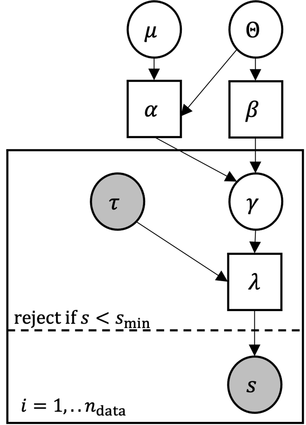
Figure 4: Gamma population hierarchical Bayesian model diagram. Circles represent random variables, boxes are deterministic quantities, and shaded variables are observed as data. The dashed line represents a possible censorship in measurement. Measurements of data $(t,s)_{i}$ are conducted until $n_{\rm data}$ samples are drawn.

Results. We display inference results in Figure 5. The Fishnets embedding (green) results in slightly inflated contours, indicating a small leakage of information. To demonstrate scaling, we additionally generate another simulation at $n_{\rm data}=10^{4}$ using the same random seed. We train another amortised posterior using 5000 simulations at $n_{\rm data}=10^{4}$ and pass the data through the same trained Fishnet architecture. The resulting posterior is shown in blue on Figure 5 for comparison.

The summaries obtained from Fishnet compression of the small data (green) result in posteriors that hug the “true” MCMC contours (black), indicating information saturation. Extending the same network on the larger data results in intuitively smaller contours (more information). It should be emphasized that $n_{\rm data}=10^{4}$ is a regime where the MCMC inference is no longer tractable on standard devices. Fishnets here allows for 1) much faster posterior calculation and 2) allows for optimal inference on larger data set sizes without any retraining.

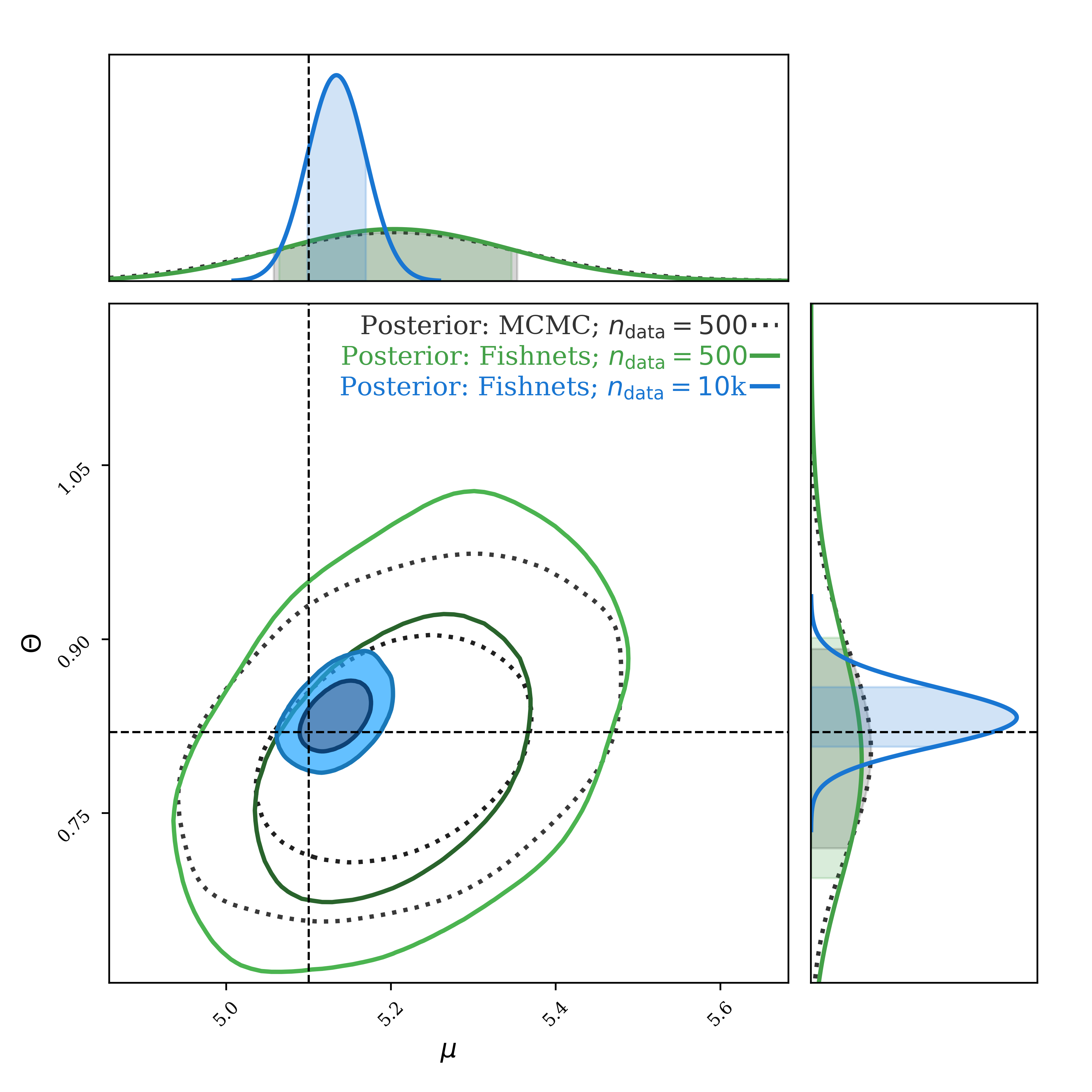
Figure 5: The same Fishnets network can be used for inference on datasets much larger than those used in training. The twin Fishnet architecture was trained on $n_{\rm data}=500$. We then compress a target dataset and perform density estimation (green) and compare to an MCMC sampler as our true posterior (black dashed). Fishnets nearly saturates the information. We then use the same network to compress simulations of $n_{\rm data}=10^{4}$ to obtain the blue contours.

As a final demonstration we solve the same problem, this time subject to censorship. In the censored case, the target joint posterior defined by the hierarchical model requires computing an integral for the selection probability as a function of the model hyper-parameters; in general, these selection terms make Bayesian problems with censorship computationally challenging, or intractable in some cases (Qi et al., 2022; Dickey et al., 1987).

We again train the Fishnets architecture on $10^{4}$ simulations of size $n_{\rm data}=500$, subject to censorship below $s_{\rm min}$. We obtain posteriors of the same shape of the censored case, but for a consistency check perform a probability-integral transform (PIT) test for the neural posterior. For each parameter we want the marginal PIT test to yield a uniform distribution to show that the learned posterior behaves as a continuous distribution. We display these results in Figure 6. We obtain a Kolmogorov-Smirnov test (Massey Jr., 1951) p-value of 0.628 and 0.233 for parameters $\mu$ and $\Theta$, respectively, indicating that our posterior is well-parameterized and robust.

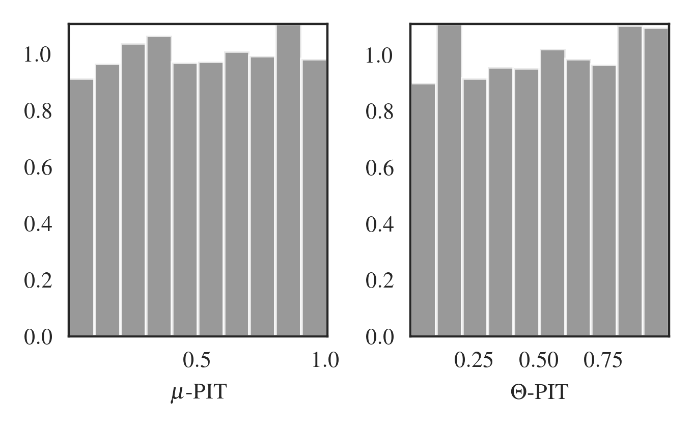
Figure 6: Density estimation posteriors obtained from parameter-Fishnets summary pairs are robust over training data for the censorship test. Each parameter’s PIT test is close to uniform, which shows that the Fishnets summary posterior has successfully captured the underlying Bayesian information from the data.

5 Graph Neural Network Aggregation

Graphs can be thought of as tuples of sets within connected neighborhoods. Graph neural networks (GNNs) operate by message-passing along edges between nodes. For predicting node- and graph-level properties, an aggregation of these sets of edges $\{e_{ij}\}$ or nodes $\{v_{i}\}$ is required to reduce features to fixed-size feature vectors.

Here we compare the Fishnets aggregation scheme as a drop-in replacement for learned softmax aggregators within the graph convolutional network (GCN) scheme presented by Li et al.. We can rewrite our aggregations to occur within neighborhoods of nodes:

$$\text{SoftmaxAgg}(\cdot) =\sum_{i\in\mathcal{N}(v)}\frac{\exp{\left(\beta\textbf{e}_{iv}\right)}}{\sum_{l\in\mathcal{N}}\exp{\left(\beta\textbf{e}_{li}\right)}}\cdot\textbf{e}_{iv},$$ (12)

$$\text{FishnetsAgg}(\cdot) =\left(\sum_{i\in\mathcal{N}(v)}\textbf{F}(\textbf{e}_{iv})\right)^{-1}\left(\sum_{i\in\mathcal{N}(v)}\textbf{t}(\textbf{e}_{iv})\right),$$ (13)

where the aggregation occurs in a neighborhood $\mathcal{N}$ of a node $v$. The Fishnets aggregation requires a bottleneck hyperparameter, $n_{p}$, which controls the size of the score embedding $\textbf{t}(\textbf{e}_{iv})\in\mathbb{R}^{n_{p}}$ and Fisher Cholesky factors $\textbf{F}_{\rm chol}\in\mathbb{R}^{n_{p}(n_{p}+1)/2}$. We use a single linear layer before aggregation to obtain score and Fisher components from hidden layer embeddings.

5.1 Testing Aggregations on ogbn-proteins Benchmark

The ogbn-proteins dataset (Hu et al., 2020, 2021) is comprised of “association scores” in eight different categories (edges) between a large set of proteins (nodes). The goal of a GNN in this benchmark is to aggregate edge association embeddings to predict protein node properties, parameterized as a 112-class categorization task. Here we expect different node neighborhoods to have a heterogenous structure across association categories, making Fishnets aggregation ideal for applicability beyond the training set.

We adopt the publicly-available Pytorch-Geometric implementation of DeeperGCN (Li et al., 2020; Fey & Lenssen, 2019), and developed a drop-in Fishnets Aggregator (in lieu of softmax aggregation) for the architecture.

We test five model architectures. As a benchmark we adopt the out-of-the-box 28-layer GCN network from (Li et al., 2020) with learned softmax aggregations and hidden size of 64, and a smaller version of this model with hidden size 14 and 28 layers. We construct two, shallower Fishnets GNNs, with 16 and 20 layers, each with 64 hidden units, and one small model with 14 hidden units and 14 layers. For each graph convolution aggregation, we adopt a “score” bottleneck of $n_{p}=10$ for the large models and $n_{p}=8$ for the small model. We train all networks with a cross-entropy loss over the same dataset and fixed random seed using an adam optimizer with fixed learning rate $0.001$. We incorporate an early stopping criterion conditioned on the validation data, which dictates an end to training (saturation) when the validation ROC-AUC metric stops increasing for $\texttt{patience}=250$ epochs.

Results. We display representative test ROC-AUC curves over training in Figure 7, and in Table 2. Fishnets-16 and Fishnets-20 clearly saturate information within 250 epochs to $79.63\%$ and $81.10\%$ accuracy respectively. The small Fishnets model saturates to $79.29\%$. The 28-layer GCN saturates the patience criterion to $79.51\%$ accuracy only after 900 epochs. This small ablation study shows that incorporating the more information-efficient Fishnets Aggregation, we can achieve better or similar results than SOTA GNNs with a fraction of the trainable parameters and training epochs (see Table 2).

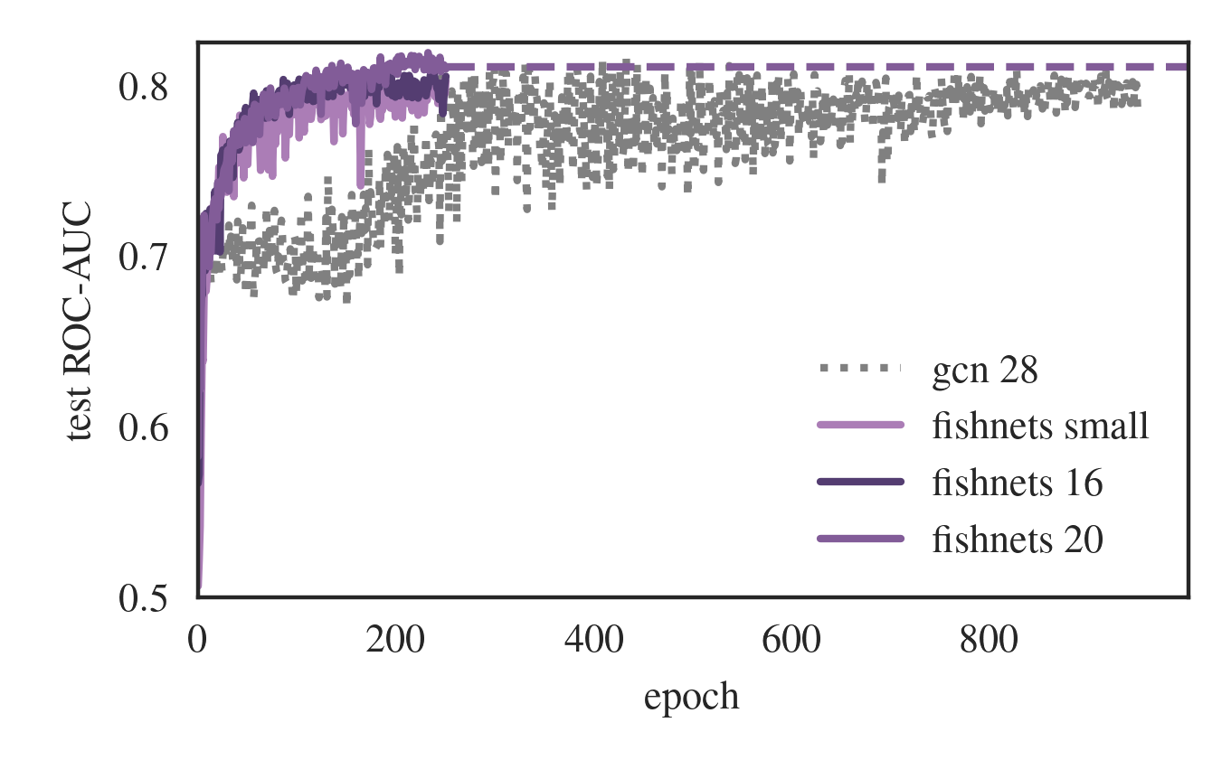
Figure 7: Drop-in replacement Fishnets aggregation improves GNN benchmark performance. We show representative test ROC-AUC curves for the benchmark proteins datasets. The dashed purple line shows our best model, Fishnet-20’s saturation point. Fishnets architectures clearly saturates the information more quickly than GCNs with learned softmax aggregations.

5.2 Modelling Uncertain Protein Associations.

As a final test, we demonstrate Fishnets aggregation for graphs in a setting with uncertainties on the protein interaction strengths (edges), in order to demonstrate the robustness of the Fishnets approach to changes in the underlying data (noise) distribution on the graph features.

We model noisy “measurements” of the protein graph edge associations using a simple Binomial model: taking the dataset edges $\textbf{p}_{ij}=\textbf{e}_{ij}\in[\textbf{0},\textbf{1}]$ as the“true” association strengths, we can simulate a noisy measurement of those quantities as $N$ weighted coin tosses per edge, where $N$ varies between measurements:

$$N\curvearrowleft\mathcal{U}(20,200)$$ (14)

$$\textbf{n}_{\rm success}\curvearrowleft\text{Binomial}\left(n=N,p=\textbf{p}_{ij}\right)$$ (15)

$$\hat{\textbf{p}}_{ij}=\textbf{n}_{\rm success}/N$$ (16)

$$\textbf{e}_{ij}\leftarrow\left[\hat{\textbf{p}}_{ij},N\right].$$ (17)

Note that in the last step the new graph edge now contains the (noisy) measured associations, as well as $N$ (which provides a measure of uncertainty on those estimated interaction strengths). The GNN task is now to learn to re-weight predictions conditioned on the provided $N$ coin toss information, much like feeding in $\sigma$ in the linear regression case. We train a 28-layer GCN and 20-layer Fishnets network on this simulated noisy version of the proteins dataset. For the test dataset, we alter the distribution for $N$ to be $\mathcal{U}(20,50)+\mathcal{U}(170,200)$ such that we sample the extremes of the training distribution support.

test	network	# params	test ROC-AUC
benchmark	fishnets-20	$442,500$	$\bm{0.8110\pm 0.0021}$
	fishnets-16	$355,584$	$0.7963\pm 0.0059$
	fishnets small	$30,360$	$0.7929\pm 0.0045$
	GCN-28	$478,092$	$0.7951\pm 0.0059$
	GCN small	$33,580$	$0.7731\pm 0.0052$
noisy edges	fishnets-20	${442,500}$	$\bm{0.7198\pm 0.0109}$
	GCN-28	$478,092$	$0.6471\pm 0.0090$

Table 2: Summary of performance on benchmark and noisy variants of the proteins dataset. Errorbars denote standard deviation of test ROC-AUC in the last ten epochs of training.

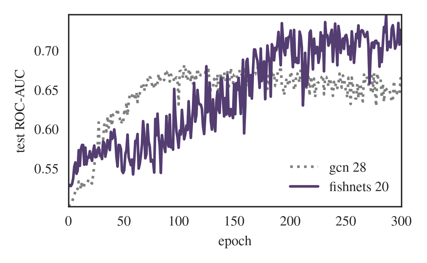
Figure 8: The Fishnets aggregation can also handle noisy edges and contextual information $N$ through explicit weight parameterization, improving the GCN result by nearly 10%.

Results. We display test ROC-AUC curves for both networks in Figure 8, subject to a patience setting of 250 epochs on the validation set. The GCN framework exhibits an early plateau at $64.71\%$ accuracy, while Fishnets saturates to $71.98\%$ accuracy. This stark difference in behaviour can be explained by the difference in formalism: The Fishnets aggregation explicitly learns a weighting scheme as a function of measured edge probabilities and the conditional information $N$, much like the linear regression case where $\sigma$ was passed as an input. This scheme helps to learn how to deal with edge-case noise artefacts like the noisy edge test case. Explicitly specifying the inverse-Fisher weighting formalism as an inductive bias (Battaglia et al., 2018) during aggregation can help explain the fast information saturation exhibited in both graph test settings.

6 Discussion & Future Work

In this paper we built up an information-theoretic approach to optimal aggregation in the form of Fishnets. Through progressively non-trivial examples, we demonstrated that explicitly parameterizing the score and inverse-Fisher weights of set members results in an aggregation scheme that saturates Bayesian information in non-trivial problems, and also serves as an optimal aggregator for graph neural networks.

The stark improvement in information saturation on the proteins test dataset relative to architecture size and training efficiency indicates that the Fishnets aggregation acts as an information-level inductive bias for GNN aggregation.

Follow-up study is warranted on optimizing hyperparameter choices for graph neural network architectures using Fishnets. We chose to demonstrate improved information capture by using an ablation study of smaller models, but careful (and potentially bigger) network design would almost certainly improve results here and potentially achieve SOTA accuracy on common benchmarks.

Code Availability

The method presented here was tested across frameworks in Tensorflow (Abadi et al., 2015), JAX (Bradbury et al., 2018), and PyTorch Geometric (Fey & Lenssen, 2019; Paszke et al., 2019). The code will be made public upon acceptance of the paper.

Appendix A Calculating the Fisher Matrix from Network Outputs

To ensure that our Fisher matrix is positive-definite, our Fisher networks output $n_{\rm params}+n_{\rm params}\frac{(n_{\rm params}+1)}{2}$ numbers as lower triangular entries in a Cholesky decomposition of the Fisher matrix, L. To ensure that the lower triangular entries remain positive-definite, we add a softplus activation to the diagonal entries of L:

$${\rm diag}(\textbf{L})\leftarrow{\rm softplus(diag(\textbf{L})}$$ (18)

We then compute the Fisher via:

$$\textbf{F}=\textbf{L}\textbf{L}^{T}$$ (19)

The negative-log likelihood loss in Equation 9 allows for explicit interrogation of the resulting Fisher matrix at the level of the predicted quantities (parameters). In the GNN regression formalism, Fishnets does not explicitly maximise the Fisher information as a part of the loss, rather the Fisher matrix weights are optimized as an inductive bias as a hidden layer in the GNN scheme.

Appendix B Experimental Details

B.1 Scalable Linear Regression

We use a toy linear regression model to validate our method and demonstrate network scalability. We consider the form $y=mx+b+\epsilon$, where $\epsilon\sim\mathcal{N}(0,\sigma)$, where the parameters of interest are the slope and intercept $\bm{\theta}=(m,b)$. This likelihood has an analytically-calculable score and Fisher matrix,

t $$=\sum_{i=1}^{n_{\rm data}}\frac{1}{\sigma_{i}^{2}}\begin{bmatrix}&x_{i}(y_{i}-(m_{\rm fid}x_{i}+b_{\rm fid}))\\ &y_{i}-(m_{\rm fid}x_{i}+b_{\rm fid}))]\end{bmatrix}+\textbf{t}_{0},$$ (20)

F $$=\sum_{i=1}^{n_{\rm data}}\frac{1}{\sigma_{i}^{2}}\begin{bmatrix}x_{i}^{2}&x_{i}\\ x_{i}&1\end{bmatrix}+\mathbf{C}^{-1}_{\rm p},$$ (21)

where $\textbf{t}_{0}=\mathbf{C}^{-1}_{\rm p}(\theta_{\rm fid}-\mu_{\rm p})$, with $\mu_{\rm p}=\textbf{0}$ is the mean of the prior on the score, and $\mathbf{C}^{-1}_{\rm p}=\textbf{I}$ is added to the Fisher matrix as a prior on the inverse-covariance of the spread of the summaries. With these two expressions we can calculate exact MLE estimates for the parameters $\bm{\theta}=(m,b)$ via Eq. (3). We choose wide Gaussian priors for $\theta$, and uniform priors for $x\in[0,10]$ and $\sigma\in[1,10]$. For network training, we simulate $10^{4}$ datasets of size $n_{\rm data}=500$ datapoints. We use fully-connected MLPs of size [256, 256, 256] with ELU activations (Clevert et al., 2015) for both score and Fisher networks. Both networks receive the input data $[y_{i},x_{i},\sigma_{i}^{2}]^{T}$. We train networks for 2500 epochs with an adam optimizer using a step learning rate decay schedule. We train an ensemble of 10 networks in parallel on the same training data with different initializations.

B.2 Robustness Network Architecture Comparison

For our three-network stress-test comparison, we construct a Fishnet, a Fishnet-Deepset (MD), and a Deepset. For the first robustness test, the Fishnet is constructed to have $[128,128,128]$ hidden units for the score and Fisher embeddings, while the Fishnet-Deepset has $[128,128,2]$ and $[128,128,3]$ embedding units and $[64,64]$ global function units. The Deepset is constructed identically to the Fishnet-Deepset, except the “Fisher” and “score” channels are concatenated together after aggregation and fed to the global function. The Deepset is then trained under typical a mean-square error loss regression to the true parameters. For the noise distribution test, we increased the width of embeddings for the two deepset networks to $[128,128,128]$ see if this provided any advantage.

B.3 Gamma Population Model

Here we detail the full implementation of the Bayesian hierarchical model validation test. Consider a serum which increases patients’ red blood cell counts, whose decay rate, $\tau$, is not known. A population of patients are injected with the serum and then asked to come back to the lab within $t_{\rm max}=10$ days for a measurement of their blood cell count, $s$. We can cast this problem using the following hierarchical model

$$\mu \curvearrowleft\mathcal{U}(0.5,10)$$

$$\Theta \curvearrowleft\mathcal{U}(0.1,1.5)$$

$$\gamma_{i} \curvearrowleft\textrm{Gamma}(\alpha=\mu/\Theta,\beta=1/\Theta)$$

$$\tau_{i} \curvearrowleft\mathcal{U}(0,10)$$

$$\lambda_{i} =A\exp(-\tau_{i}/\gamma_{i})$$

$$s_{i} \curvearrowleft\textrm{Pois}(\lambda_{i}),$$

where the goal is to infer the mean $\mu$ and scale $\Theta$ of the decay rate Gamma distribution from the data, $\{\tau_{i},s_{i}\}$. In the censored case, measurements are rejected if $s_{i}<s_{\rm min}$, and collected until $n_{\rm data}$ samples are accepted. The model is visualised in a plate diagram in Figure 4. In the uncensored case, the posterior estimation for this problem is readily solved using a high-dimensional Hamiltonian Monte-Carlo (HMC) sampler. We implement this model in Numpyro (Phan et al., 2019) as a baseline MCMC comparison for our algorithm. For the Fishnets implementation, we generate $10^{4}$ simulations of size $n_{\rm data}=500$ over a uniform prior for $\mu$ and $\Theta$. We then train the same Fishnets architecture used for the linear regression case with data inputs $[\tau_{i},s_{i}]^{T}$. Once the networks were trained, we pass a suite of $n_{\rm data}=5000$ simulations through the network to generate neural summaries with which to train a density estimation network. Following (Alsing et al., 2019), we use Mixture Density Networks to learn an amortized posterior for $p(\hat{\theta}_{\rm NN}|\theta)$ with three hidden layers of size $[50,50,50]$. We then evaluate this posterior at the same target data used for the HMC, shown in green in Figure 5. The Fishnets compression results in slightly inflated contours, indicating a small leakage of information. To demonstrate scaling, we addidionally generate another simulation at $n_{\rm data}=10^{4}$ using the same random seed. We train another amortised posterior using 5000 simulations at $n_{\rm data}=10^{4}$ and pass the data through the same trained Fishnet architecture. The resulting posterior is shown in blue for comparison.

B.4 Graph Neural Network Training

All models are implemented in PyTorch Geometric (Fey & Lenssen, 2019), and all experiments are performed on a single NVIDIA V100 32GB. ogb-proteins does not provide a node feature for each protein. We initialize the node features via a sum aggregation, e.g. $x_{i}=\sum_{j\in\mathcal{N}}$ $e_{ij}$ , where $x_{i}$ denotes the initialized node features and $e_{ij}$ denotes the input edge features.

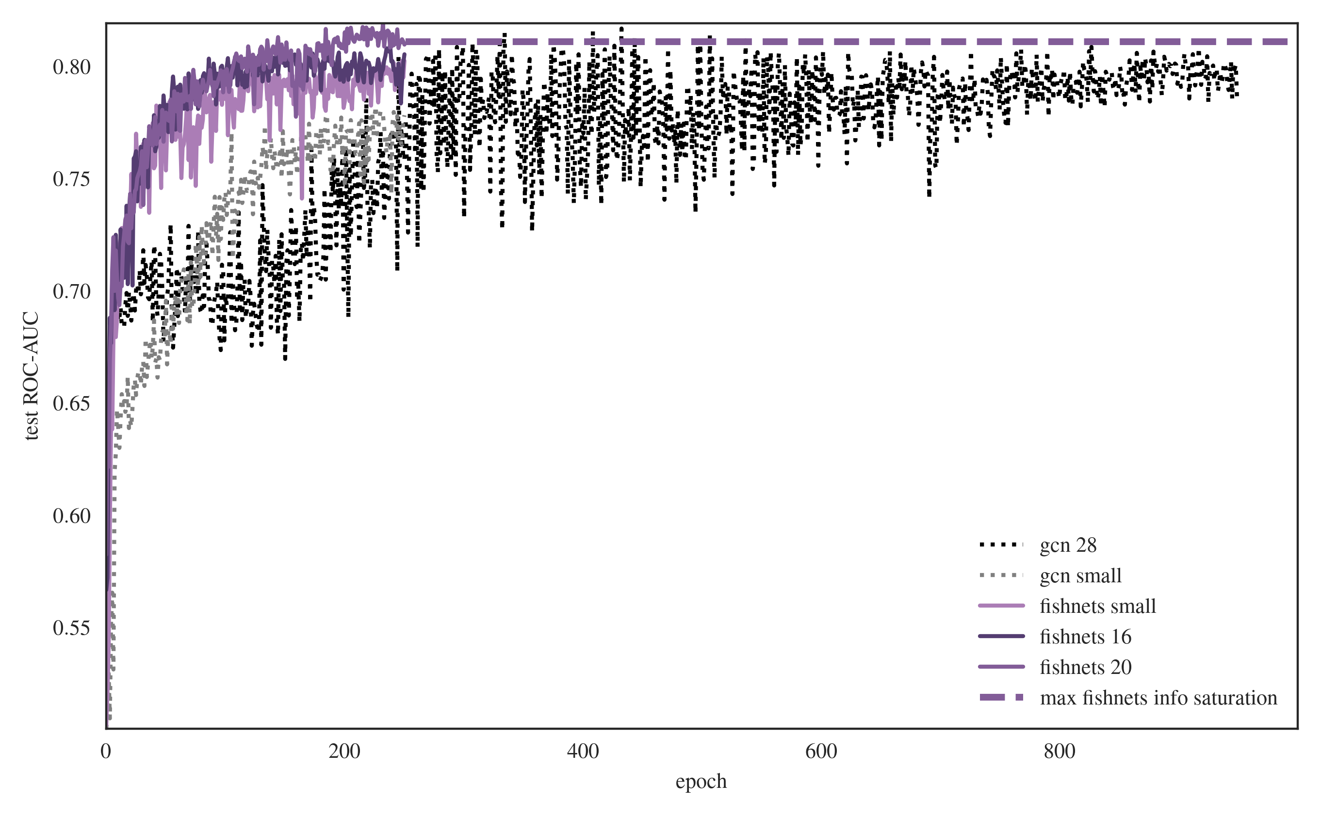
Figure 9: Zoomed-in test ROC-AUC training trajectories for models considered in benchmark ablation study on ogbn-proteins.

We test three model architectures. As a benchmark we adopt the out-of-the-box 28-layer GCN network from (Li et al., 2020) with learned softmax aggregations and hidden size of 64. We construct two, shallower Fishnets GNNs, with 16 and 20 layers, each with 64 hidden units. For each graph convolution aggregation, we adopt a “score” bottleneck of $n_{p}=10$. We connect this bottleneck to the hidden size at each GCN block by applying a linear layer to Fishnets outputs. We train all networks with a cross-entropy loss over the same dataset and fixed random seed using an adam optimizer with fixed learning rate $0.001$. We incorporate an early stopping criterion conditioned on the validation data, which dictates an end to training (saturation) when the validation ROC-AUC metric stops increasing for $\texttt{patience}=250$ epochs.

In the noisy proteins setting we again control for stochasticity in training set loading and added edge noise by fixing the initial random seed before each training run. For the test dataset, we alter the distribution for $N$ to be $\mathcal{U}(20,50)+\mathcal{U}(170,200)$ such that we sample the extremes of the training distribution support.

Appendix C Deepsets Formalism

Summary. The deepsets method presented by Zaheer et al. shows in Theorem 9 that any function over a countable set can be decomposed in the form $f(X)=\rho\left(\sum_{x\in X}\phi(x)\right)$. They then extend this to the universality of deepsets since $\rho$ and $\phi$ can be parameterized as neural networks, which can be universal function approximators. The deepsets formalism allows point-estimates for regression parameters to be obtained following an aggregation of features in a potentially variably-sized set of data. Incorporating our formalism, each set member $\textbf{d}_{i}$ is first passed to a neural network $f(\textbf{d}_{i};w_{1})$, and subsequently aggregated using some permutation-invariant scheme, $\bigoplus_{i}$.

$$\hat{\bm{\theta}}=g\left(\bigoplus_{i=1}^{n_{\rm data}}f(\textbf{d}_{i};w_{1});\ \ w_{2}\right),$$ (22)

where $f$ is the embedding network and $g$ is the “global” function that maps aggregated features to predicted parameters. When the aggregation is chosen to be the mean, the deepsets formalism is scalable to arbitrary data and becomes equivalent to the Fishnets aggregation formalism with flat weights across the aggregated data. The loss takes the form of a convex squared loss, e.g. the mean square error

$$\mathcal{L}=\frac{1}{n_{\rm batch}}\sum_{i}^{n_{\rm batch}}(\hat{\bm{\theta}}_{i}-\bm{\theta}_{i})^{2}$$ (23)

where $n_{\rm batch}$ is a batch of full simulations, each of size $n_{\rm data}$.

Training and Generalization. In practice, Deepsets requires a fixed aggregation scheme from which to learn its global function. Most often this is a summary of embedding layers $\phi(x)$. For networks to scale to arbitrary dataset cardinality, aggregations like max, mean, and variance need to be used. In a scenario where the training data distribution $p(x,\theta)$ follows a different distribution from the training data, these aggregations might pose an issue. Concretely, consider $x\sim\mathcal{N}(\mu,1)$, with the target quantity $\theta=\mu\sim\mathcal{U}(0,2)$. Next consider a deepset with the identity embedding layer $\phi(x)=x$ and mean-aggregation:

$$\hat{\mu}=\rho\left(\frac{1}{n}\sum_{i}x_{i}\right)$$ (24)

If test data $x_{i}$ were drawn from the same distribution as the test data, $\rho$ would act on the mean value of the set of data, in this case $\rho(\mathbb{E}_{p(x,\theta)}[x_{i}])$, and would produce a learned function of the joint prior-data distribution $p(x,\theta)$. However, if a test set of data were drawn from a different distribution, e.g. $\mu_{\rm test}\sim\mathcal{N}(0.5,0.1)$, then the expectation $\mathbb{E}_{p(x,\theta)}$ would take on a different value, and $\rho$ would return an incorrect result for the deterministic aggregation. Here it is important to emphasize that $p^{\rm{test}}(x,\theta)$ and $p(x,\theta)$ overlap along the same support, meaning the network will have seen examples of data drawn from this prior in the limit of an infinite training set. However, the fixed aggregation makes use of a training-data distribution-dependent quantity for its mapping, which can be skewed under covariate shift or different noise settings.

References

- Abadi et al. (2015) Abadi, M., Agarwal, A., Barham, P., Brevdo, E., Chen, Z., Citro, C., Corrado, G. S., Davis, A., Dean, J., Devin, M., Ghemawat, S., Goodfellow, I., Harp, A., Irving, G., Isard, M., Jia, Y., Jozefowicz, R., Kaiser, L., Kudlur, M., Levenberg, J., Mané, D., Monga, R., Moore, S., Murray, D., Olah, C., Schuster, M., Shlens, J., Steiner, B., Sutskever, I., Talwar, K., Tucker, P., Vanhoucke, V., Vasudevan, V., Viégas, F., Vinyals, O., Warden, P., Wattenberg, M., Wicke, M., Yu, Y., and Zheng, X. TensorFlow: Large-scale machine learning on heterogeneous systems, 2015. URL https://www.tensorflow.org/. Software available from tensorflow.org.
- Alsing & Wandelt (2018) Alsing, J. and Wandelt, B. Generalized massive optimal data compression. Monthly Notices of the Royal Astronomical Society: Letters, 476(1):L60–L64, feb 2018. doi: 10.1093/mnrasl/sly029. URL https://doi.org/10.1093%2Fmnrasl%2Fsly029.
- Alsing et al. (2019) Alsing, J., Charnock, T., Feeney, S., and Wandelt, B. Fast likelihood-free cosmology with neural density estimators and active learning. Monthly Notices of the Royal Astronomical Society, Jul 2019. ISSN 1365-2966. doi: 10.1093/mnras/stz1960. URL http://dx.doi.org/10.1093/mnras/stz1960.
- Amari (2021) Amari, S.-i. Information geometry. Japanese Journal of Mathematics, 16(1):1–48, January 2021. ISSN 1861-3624. doi: 10.1007/s11537-020-1920-5. URL https://doi.org/10.1007/s11537-020-1920-5.
- Battaglia et al. (2018) Battaglia, P. W., Hamrick, J. B., Bapst, V., Sanchez-Gonzalez, A., Zambaldi, V., Malinowski, M., Tacchetti, A., Raposo, D., Santoro, A., Faulkner, R., Gulcehre, C., Song, F., Ballard, A., Gilmer, J., Dahl, G., Vaswani, A., Allen, K., Nash, C., Langston, V., Dyer, C., Heess, N., Wierstra, D., Kohli, P., Botvinick, M., Vinyals, O., Li, Y., and Pascanu, R. Relational inductive biases, deep learning, and graph networks, 2018.
- Bradbury et al. (2018) Bradbury, J., Frostig, R., Hawkins, P., Johnson, M. J., Leary, C., Maclaurin, D., Necula, G., Paszke, A., VanderPlas, J., Wanderman-Milne, S., and Zhang, Q. JAX: composable transformations of Python+NumPy programs, 2018. URL http://github.com/google/jax.
- Charnock et al. (2018) Charnock, T., Lavaux, G., and Wandelt, B. D. Automatic physical inference with information maximizing neural networks. Physical Review D, 97(8), apr 2018. doi: 10.1103/physrevd.97.083004. URL https://doi.org/10.1103%2Fphysrevd.97.083004.
- Clevert et al. (2015) Clevert, D.-A., Unterthiner, T., and Hochreiter, S. Fast and accurate deep network learning by exponential linear units (elus), 2015. URL https://arxiv.org/abs/1511.07289.
- Corso et al. (2020) Corso, G., Cavalleri, L., Beaini, D., Liò, P., and Velickovic, P. Principal neighbourhood aggregation for graph nets. CoRR, abs/2004.05718, 2020. URL https://arxiv.org/abs/2004.05718.
- Coulton & Wandelt (2023) Coulton, W. R. and Wandelt, B. D. How to estimate fisher information matrices from simulations, 2023.
- Cramér (1946) Cramér, H. Mathematical methods of statistics, by Harald Cramer, .. The University Press, 1946.
- Cranmer et al. (2020) Cranmer, K., Brehmer, J., and Louppe, G. The frontier of simulation-based inference. Proceedings of the National Academy of Sciences, 117(48):30055–30062, may 2020. doi: 10.1073/pnas.1912789117. URL https://doi.org/10.1073%2Fpnas.1912789117.
- Dickey et al. (1987) Dickey, J. M., Jiang, J.-M., and Kadane, J. B. Bayesian methods for censored categorical data. Journal of the American Statistical Association, 82(399):773–781, 1987. ISSN 01621459. URL http://www.jstor.org/stable/2288786.
- Fey & Lenssen (2019) Fey, M. and Lenssen, J. E. Fast graph representation learning with PyTorch Geometric. In ICLR Workshop on Representation Learning on Graphs and Manifolds, 2019.
- Hamilton et al. (2017) Hamilton, W., Ying, Z., and Leskovec, J. Inductive representation learning on large graphs. In Guyon, I., Luxburg, U. V., Bengio, S., Wallach, H., Fergus, R., Vishwanathan, S., and Garnett, R. (eds.), Advances in Neural Information Processing Systems, volume 30. Curran Associates, Inc., 2017. URL https://proceedings.neurips.cc/paper_files/paper/2017/file/5dd9db5e033da9c6fb5ba83c7a7ebea9-Paper.pdf.
- Hoffmann & Onnela (2022) Hoffmann, T. and Onnela, J.-P. Minimizing the expected posterior entropy yields optimal summary statistics, 2022. URL https://arxiv.org/abs/2206.02340.
- Hu et al. (2020) Hu, W., Fey, M., Zitnik, M., Dong, Y., Ren, H., Liu, B., Catasta, M., and Leskovec, J. Open graph benchmark: Datasets for machine learning on graphs. arXiv preprint arXiv:2005.00687, 2020.
- Hu et al. (2021) Hu, W., Fey, M., Ren, H., Nakata, M., Dong, Y., and Leskovec, J. Ogb-lsc: A large-scale challenge for machine learning on graphs. arXiv preprint arXiv:2103.09430, 2021.
- Jeffrey & Wandelt (2020) Jeffrey, N. and Wandelt, B. D. Solving high-dimensional parameter inference: marginal posterior densities & amp; moment networks, 2020. URL https://arxiv.org/abs/2011.05991.
- Kipf & Welling (2017) Kipf, T. N. and Welling, M. Semi-supervised classification with graph convolutional networks, 2017.
- Li et al. (2020) Li, G., Xiong, C., Thabet, A., and Ghanem, B. Deepergcn: All you need to train deeper gcns, 2020.
- Makinen et al. (2021) Makinen, T. L., Charnock, T., Alsing, J., and Wandelt, B. D. Lossless, scalable implicit likelihood inference for cosmological fields. Journal of Cosmology and Astroparticle Physics, 2021(11):049, nov 2021. doi: 10.1088/1475-7516/2021/11/049. URL https://doi.org/10.1088%2F1475-7516%2F2021%2F11%2F049.
- Makinen et al. (2022) Makinen, T. L., Charnock, T., Lemos, P., Porqueres, N., Heavens, A. F., and Wandelt, B. D. The cosmic graph: Optimal information extraction from large-scale structure using catalogues. The Open Journal of Astrophysics, 5(1), dec 2022. doi: 10.21105/astro.2207.05202. URL https://doi.org/10.21105%2Fastro.2207.05202.
- Massey Jr. (1951) Massey Jr., F. J. The kolmogorov-smirnov test for goodness of fit. Journal of the American Statistical Association, 46(253):68–78, 1951. doi: 10.1080/01621459.1951.10500769. URL https://www.tandfonline.com/doi/abs/10.1080/01621459.1951.10500769.
- Miller et al. (2021) Miller, B. K., Cole, A., Forré, P., Louppe, G., and Weniger, C. Truncated marginal neural ratio estimation. In Ranzato, M., Beygelzimer, A., Dauphin, Y., Liang, P., and Vaughan, J. W. (eds.), Advances in Neural Information Processing Systems, volume 34, pp. 129–143. Curran Associates, Inc., 2021. URL https://proceedings.neurips.cc/paper_files/paper/2021/file/01632f7b7a127233fa1188bd6c2e42e1-Paper.pdf.
- Papamakarios et al. (2019) Papamakarios, G., Sterratt, D., and Murray, I. Sequential neural likelihood: Fast likelihood-free inference with autoregressive flows. In Chaudhuri, K. and Sugiyama, M. (eds.), Proceedings of the Twenty-Second International Conference on Artificial Intelligence and Statistics, volume 89 of Proceedings of Machine Learning Research, pp. 837–848. PMLR, 16–18 Apr 2019. URL https://proceedings.mlr.press/v89/papamakarios19a.html.
- Paszke et al. (2019) Paszke, A., Gross, S., Massa, F., Lerer, A., Bradbury, J., Chanan, G., Killeen, T., Lin, Z., Gimelshein, N., Antiga, L., Desmaison, A., Kopf, A., Yang, E., DeVito, Z., Raison, M., Tejani, A., Chilamkurthy, S., Steiner, B., Fang, L., Bai, J., and Chintala, S. Pytorch: An imperative style, high-performance deep learning library. In Advances in Neural Information Processing Systems 32, pp. 8024–8035. Curran Associates, Inc., 2019.
- Phan et al. (2019) Phan, D., Pradhan, N., and Jankowiak, M. Composable effects for flexible and accelerated probabilistic programming in numpyro. arXiv preprint arXiv:1912.11554, 2019.
- Qi et al. (2022) Qi, X., Zhou, S., and Plummer, M. On Bayesian modeling of censored data in JAGS. BMC Bioinformatics, 23(1):102, March 2022. ISSN 1471-2105. doi: 10.1186/s12859-021-04496-8. URL https://doi.org/10.1186/s12859-021-04496-8.
- Ramachandran et al. (2017) Ramachandran, P., Zoph, B., and Le, Q. V. Searching for activation functions, 2017.
- Vaart (1998) Vaart, A. W. v. d. Asymptotic Statistics. Cambridge Series in Statistical and Probabilistic Mathematics. Cambridge University Press, 1998. doi: 10.1017/CBO9780511802256.
- Veličković et al. (2018) Veličković, P., Cucurull, G., Casanova, A., Romero, A., Liò, P., and Bengio, Y. Graph attention networks, 2018.
- Wagstaff et al. (2019) Wagstaff, E., Fuchs, F. B., Engelcke, M., Posner, I., and Osborne, M. On the limitations of representing functions on sets, 2019.
- Xu et al. (2019) Xu, K., Hu, W., Leskovec, J., and Jegelka, S. How powerful are graph neural networks?, 2019.
- Zaheer et al. (2018) Zaheer, M., Kottur, S., Ravanbakhsh, S., Poczos, B., Salakhutdinov, R., and Smola, A. Deep sets, 2018.
- Zhou et al. (2020) Zhou, J., Cui, G., Hu, S., Zhang, Z., Yang, C., Liu, Z., Wang, L., Li, C., and Sun, M. Graph neural networks: A review of methods and applications. AI Open, 1:57–81, 2020. ISSN 2666-6510. doi: https://doi.org/10.1016/j.aiopen.2021.01.001. URL https://www.sciencedirect.com/science/article/pii/S2666651021000012.