Influence of disorder on antidot vortex Majorana states in 3D topological insulators

Abstract

Topological insulator/superconductor two-dimensional heterostructures are promising candidates for realizing topological superconductivity and Majorana modes. In these systems, a vortex pinned by a pre-fabricated antidot in the superconductor can host Majorana zero-energy modes (MZMs), which are exotic quasiparticles that may enable quantum information processing. However, a major challenge is to design devices that can manipulate the information encoded in these MZMs. One of the key factors is to create small and clean antidots, so that the MZMs, localized in the vortex core, have a large gap to other excitations. If the antidot is too large or too disordered, the level spacing for the subgap vortex states may become smaller than temperature. In this paper, we numerically investigate the effects of disorder, chemical potential, and antidot size on the subgap vortex spectrum, using a two-dimensional effective model of the topological insulator surface. Our model allows us to simulate large system sizes with vortices up to $1.8\,\upmu\mathrm{m}$ in diameter. We also compare our disorder model with the transport data from existing experiments. We find that the spectral gap can exhibit a non-monotonic behavior as a function of disorder strength, and that it can be tuned by applying a gate voltage.

I Introduction

Majorana zero modes (MZMs) are exotic quasiparticles that obey non-Abelian exchange statistics and can be used for topological quantum computationKitaev (2001); Nayak et al. (2008); Alicea (2012); Røising et al. (2019); Sarma et al. (2015). Topological protection is governed by the bulk excitation gap (topological gap) $\Delta_{0}$. The probability of errors induced by the local noise sources is suppressed as $\exp(-\Delta_{0}/T)$ and $\exp(-\Delta_{0}L/v)$ with $T$, $L$ and $v$ being temperature, distance between MZMs, and Fermi velocity, respectively. Another important energy scale is the minigap, which is the energy difference between the zero-energy states inside a vortex core and the higher-energy localized states. The minigap $E_{m}$ should also be larger than the temperature to enable fast and reliable measurement of the MZM parity Akhmerov (2010).

Nanowires with strong spin-orbit coupling and proximity-induced superconductivity are one of the possible platforms for creating MZMs Lutchyn et al. (2010); Oreg et al. (2010); Lutchyn et al. (2018). These nanowires can be driven into a topological phase by applying a large in-plane magnetic field. The size of the topological gap in proximitized nanowires depends on several factors, such as the spin-orbit coupling strength, the superconducting gap of the parent material, and the Zeeman energy induced by the magnetic field Lutchyn et al. (2010); Oreg et al. (2010); Lutchyn et al. (2018). A recent experiment reported a topological phase transition with a topological gap of several tens of $\upmu$eV in gate-defined proximitized nanowires Aghaee et al. (2023). However, this platform requires very high-quality nanowires with a localization length larger than one micron, which poses significant challenges for fabrication Aghaee et al. (2023).

Another promising platform for MZMs is the surface of a three-dimensional topological insulator (3D TI) covered by a superconductor (SC) Fu and Kane (2008). This platform does not require a large magnetic field, as the surface of the 3D TI naturally realizes topological superconducting state that can host MZMs in vortices Jauregui et al. (2018); Rosen et al. (2021); Rüßmann and Blügel (2022). A possible way to create and control vortices is to use an antidot structure, where part of the SC is removed, as shown in Fig. 1a. The size of the antidot can be chosen such that a small magnetic field can induce a vortex with a single MZM. For a large antidot, the magnetic flux quantum required for a MZM can then be achieved with a relatively small magnetic field. This should be contrasted with recently studied zero modes in Abrikosov vortices at high magnetic fields in Fe-based type-II superconductors (typically a few tesla) Kong et al. (2019); Chiu et al. (2020) or in proximitized topological insulator surfaces (at fields of order $0.1\,\mathrm{T}$) Xu et al. (2015); Sun et al. (2016). Moreover, the electron density inside the antidot can be tuned by a gate voltage, since it is not screened by the SC Lee (2020). Despite the advantages of this platform, there are still many open questions and challenges that need to be addressed. Most of the previous studies on the 3D TI antidot structure have focused on either the clean Akzyanov et al. (2014); Deng et al. (2020); Ziesen and Hassler (2021) or the strongly disordered Ioselevich et al. (2012) regimes, where analytical results can be obtained. However, these regimes may not be relevant for realistic experiments, where intermediate disorder strengths and finite system sizes are more common. Therefore, numerical simulations are needed to provide more accurate predictions and guidance for experimental works regarding disorder requirements.

Recently, Ref. Ziesen et al. (2023) performed a numerical study of the low-energy antidot subgap spectrum using an effective model that treats the SC outside the antidot as a boundary condition for the 3D TI surface. In this paper, we present a more realistic modeling of the antidot structure using a two-dimensional (2D) effective model for the proximitized 3D TI surface, which we describe in Sec. II. This model allows us to simulate large system sizes up to $3.6\,\upmu\mathrm{m}\times 3.6\,\upmu\mathrm{m}$ with a lattice spacing $a=6\,\mathrm{nm}$, and to capture the low-energy physics near the Dirac point. We investigate how the minigap depends on various parameters, such as disorder strength, antidot radius, and chemical potential (i.e., electron density), in Sec. III. We also compare our disorder model with experimental mobility data to estimate realistic disorder levels in existing materials. We discuss the implications of our results for the feasibility of observing MZMs in this platform in Sec. IV.

II Model

II.1 Effective model of the proximitized TI surface

To be able to efficiently simulate a 2D surface of a 3D TI with a single Dirac cone, we utilize an effective square-lattice model of the surface that breaks global time-reversal symmetry Pikulin and Franz (2017); Marchand and Franz (2012). Within this model, the Hamiltonian of a uniform surface has the form

$$h_{\mathrm{TI}}(\mathbf{k})=\lambda(s_{x}\sin ak_{x}+s_{y}\sin ak_{y})+M_{\mathbf{k}}s_{z}-\mu,$$ (1)

where $M_{\mathbf{k}}=m\bigl{(}\frac{3}{2}-\cos ak_{x}-\cos ak_{y}+\frac{1}{4}\cos 2ak_{x}+\frac{1}{4}\cos 2ak_{y}\bigr{)}$ is the time-reversal symmetry breaking term, $s_{i}$ are Pauli matrices in the spin space, $k_{i}$ are electronic momenta, $a$ is the lattice spacing, and $\mu$ is the chemical potential. In the absence of $M_{\mathbf{k}}$, the Hamiltonian has four Dirac cones at the high symmetry points $\Gamma=\left(0,0\right)$, $\mathrm{X}=\left(\frac{\pi}{a},0\right)$, $\mathrm{Y}=\left(0,\frac{\pi}{a}\right)$, and $\mathrm{M}=\left(\frac{\pi}{a},\frac{\pi}{a}\right)$; the model parameter $\lambda$ determines the Dirac velocity, $v_{D}=\lambda a/\hbar$. The term $M_{\mathbf{k}}$ breaks the global time-reversal symmetry and opens gaps of the order of $|m|$ at all high symmetry points except for $\Gamma$, where its effect on the Dirac spectrum is minor, given that $M_{\mathbf{k}}\approx\frac{ma^{4}}{8}(k_{x}^{4}+k_{y}^{4})$ for small $\mathbf{k}$. The presence of the term $M_{\mathbf{k}}$ thus effectively creates a 2D surface with a single Dirac cone at $\Gamma$. We refer the reader to Ref. Pikulin and Franz, 2017 for a detailed description of the model.

Proximity-induced superconductivity is included by constructing a Bogoliubov-de Gennes Hamiltonian $H=\frac{1}{2}\sum_{\mathbf{k}}\Psi^{\dagger}_{\mathbf{k}}H_{\mathrm{BdG}}(\mathbf{k})\Psi_{\mathbf{k}}$ with

$$H_{\mathrm{BdG}}(\mathbf{k})=\begin{pmatrix}h_{\mathrm{TI}}(\mathbf{k})&i\Delta s_{y}\\ -i\Delta^{*}s_{y}&-h^{*}_{\mathrm{TI}}(-\mathbf{k})\\ \end{pmatrix},$$ (2)

where $\Delta$ is the proximity-induced SC pairing potential and the basis spinor is $\Psi_{\mathbf{k}}^{\dagger}=(c^{\dagger}_{\uparrow,\mathbf{k}},c^{\dagger}_{\downarrow,\mathbf{k}},c_{\uparrow,-\mathbf{k}},c_{\downarrow,-\mathbf{k}})$.

In our simulations we choose a discretization with the lattice spacing $a=0.03\pi\xi_{0}$, where $\xi_{0}=\hbar v_{D}/(\pi\Delta_{0})$ is the superconducting coherence length in a clean proximitized system, and $\Delta_{0}$ denotes the induced SC gap. By definition, $\lambda=\pi\Delta_{0}\xi_{0}/a$. Furthermore, we fix $m=-1.5\lambda$ (the choice of sign is arbitrary). As demonstrated in Appendix A, up to energies $|E|\ll 60\Delta_{0}$ the term linear in $\mathbf{k}$ in the power series expansion of (1) dominates over higher order terms. Therefore, in the energy range investigated in this work ($|E|\leq 15\Delta_{0}$), our lattice model is a good approximation of the TI surface Dirac Hamiltonian.

We note that, when $|\Delta_{0}|\ll|m|$ and $|\mu|\ll|m|$, the model has a non-zero Chern number $C=\mathrm{sign}(m)$, which is due to the presence of time-reversal symmetry breaking terms in (2). Hence, our finite-size system with open boundary conditions will feature a chiral edge mode, which is an artifact of the effective model. Effectively, the edge of the sample is analogous to a boundary between a SC-proximitized TI surface and a magnetic-insulator-proximitized TI surface with Chern number $C=-\mathrm{sign}(m)$. In the following simulations the edges are located at least $12\xi_{0}$ away from the antidot boundary. This ensures that the spurious edge states have negligible influence on the antidot spectrum.

II.2 Model of the antidot system

To simulate the antidot device, we write the Hamiltonian (2) in the position space, and allow spatial variation of the chemical potential $\mu$ and the pairing potential $\Delta$. Spatial variation of $\lambda$, which could emerge due to the proximity-induced renormalization of $v_{D}$, is neglected.

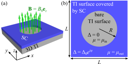
Figure 1: (a) Sketch of the sample structure and the modeled distribution of the magnetic field. (b) Top view of the sample with a schematic representation of the parameters of the model.

A schematic sketch of the modeled sample is shown in Fig. 1. The system comprises a square fragment of a 3D TI surface with a side length of $L=3.6\,\upmu\mathrm{m}$, covered by a SC layer everywhere except for a circular antidot area of radius $R$ in the middle. We fix the coordinate system origin in the center of the antidot and denote $(r,\varphi)$ as polar coordinates. We assume that the magnetic field is present exclusively in the antidot area and has the form

$$\mathbf{B}(\mathbf{r})=\begin{cases}(0,0,B_{0})&\textrm{for }r<R,\\ (0,0,0)&\textrm{for }r\geq R,\\ \end{cases}$$ (3)

which is a valid approximation in the case of a thick superconductor with a short London penetration length. We choose $B_{0}=\Phi_{0}/(\pi R^{2})$, such that the sample is permeated by a single flux quantum $\Phi_{0}=h/(2|e|)$. The magnetic vector potential compatible with the assumed magnetic field distribution is expressed in the London gauge as

$$\mathbf{A}(\mathbf{r})=\begin{dcases}\frac{\Phi_{0}}{2\pi R^{2}}(-y,x,0)&\textrm{for }r<R,\\ \frac{\Phi_{0}}{2\pi r^{2}}(-y,x,0)&\textrm{for }r\geq R.\\ \end{dcases}.$$ (4)

The flux trapped by the antidot induces a phase winding of the pairing potential

$$\Delta(\mathbf{r})=\begin{cases}0&\textrm{for }r<R,\\ \Delta_{0}e^{-i\varphi}&\textrm{for }r\geq R,\\ \end{cases}.$$ (5)

Furthermore, the vector potential $\mathbf{A}(\mathbf{r})$ is introduced into the hopping terms via the Peierls substitution,

$$c^{\dagger}_{\mathbf{r}_{1}}c_{\mathbf{r}_{0}}\rightarrow c^{\dagger}_{\mathbf{r}_{1}}c_{\mathbf{r}_{0}}\exp\left(-i\frac{|e|}{\hbar}\int_{L_{01}}\mathbf{A}(\mathbf{r})\cdot d\mathbf{r}\right),$$ (6)

where $L_{01}$ is the straight line pointing from $\mathbf{r}_{0}$ to $\mathbf{r}_{1}$.

The chemical potential profile is made up of two parts: $\mu(\mathbf{r})=\mu_{0}(\mathbf{r})+\delta\mu(\mathbf{r})$. The first part describes an idealized impurity-free sample, while the second part represents the effect of the disorder. We assume that the chemical potential is fixed in the SC part of the system, while in the antidot it can be controlled by gating, and write

$$\mu_{0}(\mathbf{r})=\begin{cases}\mu_{\textrm{in,0}}&\textrm{for }r<R,\\ \mu_{\textrm{out}}&\textrm{for }r\geq R.\\ \end{cases}$$ (7)

II.3 Disorder model and its relation to the scattering rate

The disorder in the system is modeled by distributing $2N_{C}$ charged impurities at randomly chosen distinct lattice sites $\mathbf{r}^{C}_{n}$ throughout the sample. The charges have equal magnitude, although half of them are negative and half are positive, such that the net charge in the system is exactly zero, and the correction to the chemical potential due to disorder is

$$\delta\mu(\mathbf{r})=\sum_{n=1}^{N_{C}}V(\mathbf{r}-\mathbf{r}^{C}_{n})-\sum_{n=N_{C}+1}^{2N_{C}}V(\mathbf{r}-\mathbf{r}^{C}_{n}).$$ (8)

As our TI surface model (1) features spin-polarized bands away from $\Gamma$, the disorder-induced scattering could potentially generate a magnetic gap in the surface Dirac spectrum. To avoid this issue, we choose the single impurity potential $V(\mathbf{r})$ to have a Gaussian profile, such that the high momentum scattering is suppressed. The model potential in (8) is assumed to have the form

$$V(\mathbf{r})=-\frac{V_{0}}{\sqrt{\mathcal{N}}}\exp\left(-\frac{\mathbf{r}^{2}}{2\sigma^{2}}\right),$$ (9)

where $V_{0}$ is the magnitude of the potential, while $\sigma$ gives the radius of the potential well, and $\mathcal{N}=\sum_{i\in\textrm{lattice}}\exp[-\mathbf{r}_{i}^{2}/\sigma^{2}]$ is the normalization factor designed to fix the variance of $V(\mathbf{r})$ at the lattice sites $\mathbf{r}_{i}$ such that $\sum_{i\in\textrm{lattice}}V^{2}(\mathbf{r}_{i})=V_{0}^{2}$. The parameter $\sigma^{-1}$ gives an estimate for the largest momentum change in the scattering process. We fix $\sigma=2.5a$ in all calculations, for which choice the sum can be approximated by an integral and $\mathcal{N}\approx\pi(\sigma/a)^{2}$.

Finally, we connect the abstract parameters of the numerical model with measurable disorder characteristics. For $\mu_{0}=0$ we estimate the electron elastic scattering rate, averaged over fluctuations of $\delta\mu$, to be

$$\Gamma=\left\langle\frac{\hbar}{\tau_{\mathbf{k}}}\right\rangle_{\delta\mu}=\sqrt{8\pi}\frac{\sigma^{2}s^{3}}{\hbar^{2}v_{D}^{2}}\left(1-2\frac{\sigma^{2}s^{2}}{\hbar^{2}v_{D}^{2}}\right),$$ (10)

where

$$s^{2}=\rho_{\mathrm{imp}}\frac{V^{2}_{0}\pi\sigma^{2}}{\mathcal{N}}\approx\rho_{\mathrm{imp}}V^{2}_{0}a^{2}$$ (11)

is the estimated variance of $\delta\mu(\mathbf{r})$ at fixed $\mathbf{r}$. Expression (10) is valid if $|\delta\mu|\ll|\hbar v_{D}/\sigma|$ everywhere in the sample. For stronger disorder, and for $\mu_{0}\neq 0$, we evaluate $\Gamma$ numerically. See Appendix B for the derivations of both the approximate and the numerical approaches and a plot of the dependence $\Gamma(s)$. Finally, we estimate the electron mean free path as

$$l=v_{D}\left\langle\frac{1}{\tau_{\mathbf{k}}}\right\rangle_{\delta\mu}^{-1}=\frac{\hbar v_{D}}{\Gamma}.$$ (12)

III Results

Our main objective is to investigate how the minigap and the local density of states change upon introducing disorder in the sample. To that end, we calculated the energy spectrum of the antidot system, while varying the impurity potential magnitude $V_{0}$ and the impurity density $\rho_{\mathrm{imp}}$. In addition, we considered different values of the antidot radius $R$ and of the chemical potential $\mu_{\mathrm{in,0}}$ inside the sample, as these are the degrees of freedom that can be controlled directly in experiment. While in principle the results depend on the details of the distribution of impurities, we present the data calculated for a specific, representative realization of disorder. Thus, we capture the qualitative features of the investigated phenomena, whereas the quantitative details are to be understood as coarse estimates.

We characterize the antidot system with dimensionless quantities $\mu/\Delta_{0}$, $R/\xi_{0}=\pi R\Delta_{0}/(\hbar v_{D})$, and $V_{0}/\Delta_{0}$. Furthermore, we fix the chemical potential in the SC part of the system to be $\mu_{\mathrm{out}}=2\Delta_{0}$. We have verified numerically that varying $\mu_{\mathrm{out}}$ in the range of several $\Delta_{0}$ has a negligible effect on the minigap, although the energies of higher excited states can be affected more significantly.

First, we consider a fixed impurity density $\rho_{\mathrm{imp}}\xi_{0}^{2}\approx 17$, which in our model corresponds to the fraction of 0.15 of the lattice sites being occupied by impurities, and two different antidot radii: $R=1.26\pi\xi_{0}\approx 4\xi_{0}$ and $R=4.5\pi\xi_{0}\approx 14\xi_{0}$. The smaller (larger) value of $R$ represents the regime in which the antidot area constitutes the minority (majority) of the area $\approx\pi(R+\pi\xi_{0})^{2}$ occupied by the wave functions of states bound to the vortex core. The specific numerical values of $R$ are dictated by the convenience of numerical calculations. In Figure 2(a,b) we present the calculated energy spectra for the two antidot sizes, where the magnitude of the impurity potential $V_{0}$ is varied from $0$ to $15\Delta_{0}$ for the smaller antidot, and from $0$ to $8.2\Delta_{0}$ for the larger one. For the chosen impurity density these ranges correspond to $\Gamma$ changing from $0$ to $4.3\Delta_{0}$ and from $0$ to $0.8\Delta_{0}$, respectively. The introduction of the disorder potential $\delta\mu(\mathbf{r})$ in the numerical model leads to a shift in the average of the chemical potential inside the antidot:

$$\langle\mu_{\mathrm{in}}\rangle=\mu_{\mathrm{in,0}}+\frac{1}{\pi R^{2}}\int_{r<R}\delta\mu(\mathbf{r})\,d^{2}\mathbf{r}.$$ (13)

We account for this effect by adjusting $\mu_{\mathrm{in,0}}$ such that $\langle\mu_{\mathrm{in}}\rangle=0$ in every calculation.

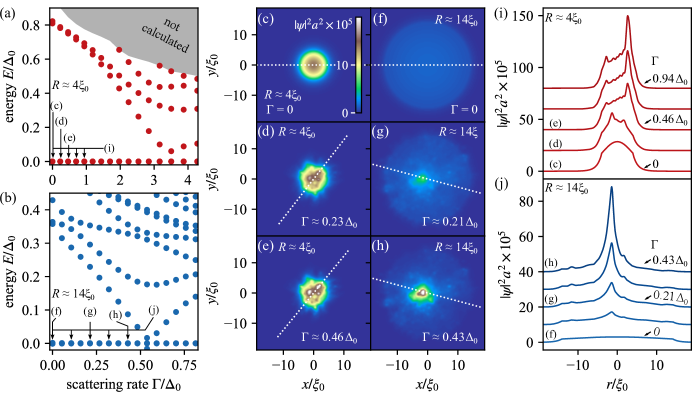
Figure 2: Left column: Energy spectra of the vortex cores pinned inside the antidots of radii (a) $R\approx 4\xi_{0}$ and (b) $R\approx 14\xi_{0}$ plotted as functions of the disorder scattering rate $\Gamma$, obtained by fixing the distribution of impurities at density $\rho_{\mathrm{imp}}\approx 17/\xi_{0}^{2}$ and by tuning the parameter $V_{0}$ in (9). Central column: Density maps of the MZM wave functions’ squared moduli in the antidots of radii (c-e) $R\approx 4\xi_{0}$ and (f-h) $R\approx 14\xi_{0}$, calculated (c,f) without disorder, and (d,e,g,h) with disorder with the scattering rate indicated in the plots. The color scale in (c) is common for all maps (c-h). Right column: Radial profiles of the MZM wave functions’ squared moduli, drawn along the lines crossing the density maxima [shown as dotted lines in (c-h)] for the antidots of radii (i) $R\approx 4\xi_{0}$ and (j) $R\approx 14\xi_{0}$, obtained for several values of $V_{0}$ corresponding to evenly spaced values of $\Gamma$ corresponding to arrows in (a,b). Vertical spacing of (i) $2\times 10^{6}$ or (j) $1\times 10^{6}$ has been applied to the baselines of the curves to enhance clarity of the data.

For both antidot radii we find that the minigap decreases approximately linearly with increasing $\Gamma$, and attains a minimum at a certain critical value $\Gamma_{c}$, but does not reach zero due to the finite size of the antidot. At the same time, the MZM wave function changes its distribution with growing $\Gamma$, as illustrated in Figure 2(c-j). In the case of a clean sample, the MZM wave function is smooth in the entire antidot area and distributed symmetrically along the polar axis around the antidot center. This is due to $\langle\mu_{\mathrm{in}}\rangle$ being fixed at the charge neutrality point of the TI surface Dirac spectrum. At $\Gamma>0$ the wave function, albeit still permeating the whole antidot, develops maxima at certain randomly located points. Figure 2(c-h) shows the wave function density maps for values of $\Gamma$ varied between $0$ and $0.5\,\Delta_{0}$, such that the minigap is open. The square moduli of the MZM wave function presented in the Figure are equivalent to the local density of states (LDOS) profiles, as the MZM is the only state within the $0.1\Delta_{0}$ range of zero energy. In Figure 2(i,j) we present cross sections through the LDOS profiles for several more values of $\Gamma$.

We complement the above results obtained for a fixed value of $\rho_{\mathrm{imp}}$ and variable $V_{0}$ with a series of calculations performed for fixed $V_{0}=6\Delta_{0}$ and changing $\rho_{\mathrm{imp}}$ with values ranging from 0 up to $\rho_{\mathrm{imp}}\xi^{2}_{0}\approx 20$, which corresponds to $\Gamma$ ranging from $0$ to $0.43\Delta_{0}$. The energy spectra calculated for the two antidot radii, $R\approx 4\xi_{0}$ and $R\approx 14\xi_{0}$, are presented in Fig. 3(a,b). The results for subsequent values of $\rho_{\mathrm{imp}}$ were obtained by successively adding impurity sites to the system, such that all impurity locations at a given value of $\rho_{\mathrm{imp}}$ are preserved in calculations for all larger $\rho_{\mathrm{imp}}$ values. We allowed the new impurity sites to fall both inside and outside of the antidot. At each step $\mu_{\mathrm{in,0}}$ was adjusted according to Eq. (13) such that $\langle\mu_{\mathrm{in}}\rangle=0$ at all times. Similarly to the case of fixed $\rho_{\mathrm{imp}}$ and variable $V_{0}$ described in Fig. 2, here we find that the decrease of the minigap with growing $\Gamma$ is approximately linear, albeit with some fluctuations which we attribute to the randomness of the process of increasing the impurity density.

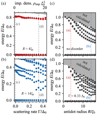
Figure 3: Left column: Energy spectra of the vortex cores pinned inside the antidots of radii (a) $R\approx 4\xi_{0}$ and (b) $R\approx 14\xi_{0}$ as functions of the disorder scattering rate $\Gamma$, obtained by changing the impurity density $\rho_{\mathrm{imp}}$ with a fixed single-impurity potential magnitude $V_{0}=6\Delta_{0}$. Right column: Analogous energy spectra as functions of the antidot radius (c) without disorder and (d) with disorder characterized by parameters $V_{0}=6\Delta_{0}$ and $\rho_{\mathrm{imp}}\approx 17/\xi_{0}^{2}$.

Our findings consistently indicate that the energy spectrum of the smaller antidot is less susceptible to disorder. The calculated dependence of the spectrum on the antidot radius is presented in Fig. 3(c) for the case of a clean sample, and Fig. 3(d) for the disordered one with a fixed disorder profile. In the case of no disorder, the minigap decreases monotonically, and at $R\gg\xi_{0}$ becomes inversely proportional to $R$, while in the limit $R\rightarrow 0$ it saturates to a finite value. For the disordered case with $\Gamma/\Delta_{0}\approx 0.33$, the decrease of minigap is not monotonic, which is due to the impurities being localized at random locations in the sample. As $R$ is increased, more and more impurity sites fall within the antidot area, and the mean value of $\delta\mu$ in the antidot fluctuates. At each step $\mu_{\mathrm{in,0}}$ was adjusted such that $\langle\mu_{\mathrm{in}}\rangle=0$. We find that the decrease of the minigap with growing $R$ is more significant in the disordered sample than in the clean sample. Comparing Figs. 3(c) and 3(d), we conclude that antidots with the radius near $\pi\xi_{0}$ are not significantly affected by disorder and are thus favourable for potential applications in topological quantum computation.

So far we have adopted a fixed average chemical potential $\langle\mu_{\mathrm{in}}\rangle=0$, although in a real device it would generally attain a different value determined by the specific properties of the materials comprising the heterostructure and its fabrication quality. However, it is our assumption that $\langle\mu_{\mathrm{in}}\rangle$ can be effectively controlled by an external electric field through tuning $\mu_{\mathrm{in,0}}$ in (13). This could be achieved by introducing a gate terminal adjacent to the heterostructure in the vicinity of the antidot. Thus, in a given sample, one would ideally be able to optimize the minigap size by tuning the gate voltage. Additional tuning can be achieved by using multiple gates Ziesen et al. (2023).

In Fig. 4(a-d) we present the energy spectra of the antidots of radii $R\approx 4\xi_{0}$ and $R\approx 14\xi_{0}$ plotted as functions of $\langle\mu_{\mathrm{in}}\rangle$, which is varied in the range of a few $\Delta_{0}$. Fig. 4(a-b) presents the results for clean samples, confirming that in fact $\langle\mu_{\mathrm{in}}\rangle/\Delta_{0}\approx 0$ corresponds to the largest minigap. Note that the plotted spectra are not symmetric with respect to $\langle\mu_{\mathrm{in}}\rangle=0$, which is due to the chemical potential $\mu_{\mathrm{out}}$ outside the antidot having a non-zero value.

In the presence of disorder with $\Gamma\approx 0.33\Delta_{0}$ (as calculated at $\langle\mu_{\mathrm{in}}\rangle=0$), the two samples with different radii respond differently to adjusting $\langle\mu_{\mathrm{in}}\rangle$. Fig. 4(c) shows that for the antidot with $R\approx 4\xi_{0}$ the optimal minigap again occurs at $\langle\mu_{\mathrm{in}}\rangle/\Delta_{0}\approx 0$. On the contrary, the spectrum of the disordered antidot with $R\approx 14\xi_{0}$ features states lying in the gap of the clean system. Due to their presence, $\langle\mu_{\mathrm{in}}\rangle/\Delta_{0}$ corresponding to the optimal minigap is clearly shifted away from zero.

For $|\langle\mu_{\mathrm{in}}\rangle|$ above a certain value, both in the clean and the disordered system, the minigap nearly closes, and the spectrum can feature densely spaced energy levels corresponding to trivial Caroli-de Gennes-Matricon (CdGM) states bound to the vortex core localized inside the antidot. This is consistent with scanning tunneling microscopy and spectroscopy (STM/STS) experiments with Abrikosov vortices in SC-TI heterostructures, where the bound states manifest themselves as an apparent splitting of the zero-bias peak at a certain distance from the vortex core Xu et al. (2015).

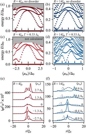
Figure 4: The influence of the chemical potential on the energy spectra of the vortex cores pinned inside the antidots of radii (a,c,e) $R\approx 4\xi_{0}$ and (b,d,f) $R\approx 14\xi_{0}$. The spectra are plotted as functions of the mean chemical potential in the antidot $\langle\mu_{\mathrm{in}}\rangle$, both (a,b) in clean systems and (c,d) in systems with disorder characterized by parameters $V_{0}=6\Delta_{0}$ and $\rho_{\mathrm{imp}}\approx 17/\xi_{0}^{2}$, which at $\langle\mu_{\mathrm{in}}\rangle=0$ corresponds to $\Gamma\approx 0.33\Delta_{0}$. (e,f) Radial profiles of the MZM wave functions squared moduli, corresponding to states indicated by black arrows in (a-d). Dashed (solid) lines present the results for the clean (disordered) systems. To enhance the clarity of the data vertical spacing of (e) $1\times 10^{7}$ or (f) $3\times 10^{6}$ has been applied to the baselines of the curves. Dashed lines in (f) represent original data multiplied by a factor of 2.

Importantly, tuning the chemical potential $\langle\mu_{\mathrm{in}}\rangle$ also results in the change of the MZM wave function distribution. In a clean sample at $\langle\mu_{\mathrm{in}}\rangle=0$ the MZM is almost evenly distributed throughout the antidot area and spills into the surrounding SC region with an exponentially decreasing amplitude. For non-zero $\langle\mu_{\mathrm{in}}\rangle$, however, the MZM density develops a distinct peak at the vortex core. The radial profiles of the MZMs in clean samples are shown as dashed lines in Fig. 4(e,f). In the disordered antidots case, on the other hand, the MZMs exhibit spatial fluctuations and peaks at random points, even at $\langle\mu_{\mathrm{in}}\rangle=0$. Upon the variation of the chemical potential, the spatial profile of the wave function is altered, such that the existing peaks level off, and the new peaks emerge at different locations. The MZMs in disordered samples are represented by solid lines in Fig. 4(e,f). Such variation of the wave functions both in the clean and the disordered case can be attributed to the change of the Fermi momentum $k_{F}\approx\langle\mu_{\mathrm{in}}\rangle/(\hbar v_{D})$ in the TI surface with the changing chemical potential, and the associated change of the density of states per unit area $\rho_{\mathrm{TI}}\approx|\langle\mu_{\mathrm{in}}\rangle|/(2\pi\hbar^{2}v_{D}^{2})$. At larger $|\langle\mu_{\mathrm{in}}\rangle|$, states from a larger Fermi contour of the TI surface spectrum contribute to the formation of the MZM, allowing a tighter peak of the MZM amplitude near the vortex core in clean samples. In disordered samples the scattering from impurities obscures this effect. However, the change of the make-up of the Fermi contour with changing $\langle\mu_{\mathrm{in}}\rangle$ results in the MZM wave functions exhibiting different interference patterns. We propose that the evolution of the MZM wave function upon varying the gate voltage can be observed by means of the STM/STS method.

The above results motivate a comprehensive study of the antidot with the smallest meaningful size, which is estimated by the radius of the core of an Abrikosov vortex $\approx\xi_{0}$. We expect that the disorder magnitudes allowed by our model have a minor effect on the spectra of such systems. Instead, we focus on the case of $R=0.8\pi\xi_{0}\approx 2.5\xi_{0}$, which is closer to the theoretical limit than the previously investigated radii. We calculate the minigap as a function of both the chemical potential inside the antidot $\langle\mu_{\mathrm{in}}\rangle$ and the impurity potential strength $V_{0}$, for a fixed impurity density $\rho_{\mathrm{imp}}\approx 17/\xi_{0}^{2}$. The results are shown as a color map in Fig. 5, with the disorder strength expressed as the scattering rate $\Gamma$ calculated for the chemical potential tuned to the Dirac point of the TI surface states ($\langle\mu_{\mathrm{in}}\rangle=0$).

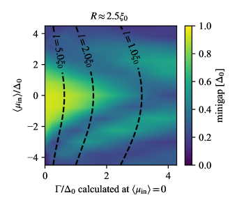
Figure 5: A color map of the minigap value for the antidot of radius $R\approx 2.5\xi_{0}$ as a function of the chemical potential inside the antidot $\langle\mu_{\mathrm{in}}\rangle$ and the disorder strength. The disorder strength is tuned by varying the parameter $V_{0}$ between $0$ and $15\Delta_{0}$ with a fixed distribution of impurities of density $\rho_{\mathrm{imp}}\approx 17/\xi_{0}^{2}$, and expressed in terms of the scattering rate $\Gamma$ calculated at $\langle\mu_{\mathrm{in}}\rangle=0$. Black dashed lines are constant $\Gamma$ contours and are labeled by the associated values of the mean free path $l=\hbar v_{D}/\Gamma$.

Note that a uniform change of $\langle\mu_{\mathrm{in}}\rangle$, e.g., by applying gate voltage, corresponds to a vertical displacement in the plot in Fig 5. However, such a process would result in a change of measured $\Gamma$, since the density of states depends on $\langle\mu_{\mathrm{in}}\rangle$. For reference, contours denoting selected values of $\Gamma$ for arbitrary $\langle\mu_{\mathrm{in}}\rangle$ are included in Fig. 5 as black dashed lines and labeled with the associated value of the mean free path (12).

Noticeably, vertical linecuts of the data presented in Fig. 5 agree in qualitative terms with analogous spectra shown in Fig. 4(a-d), obtained by fixing the disorder magnitude and varying $\langle\mu_{\mathrm{in}}\rangle$. Similarly, the horizontal linecut for $\langle\mu_{\mathrm{in}}\rangle=0$ is in agreement with the analogous data in Fig. 2(a-b). Very clearly, the minigap decreases both with growing $|\langle\mu_{\mathrm{in}}\rangle|$ and growing $\Gamma$, albeit with significant oscillations. Therefore, for a given disordered sample, a wide scan of $\langle\mu_{\mathrm{in}}\rangle$ has to be performed to find the configuration ensuring the maximal value of the minigap.

IV Conclusions

We performed a detailed numerical analysis of the TI-SC device with an antidot structure, using realistic parameters. We focused on how the minigap, which separates the zero-energy Majorana mode in the antidot from the first excited trivial CdGM state, depends on various factors, i.e. geometrical dimensions, Fermi energy, and disorder strength. We also examined how these factors affect the Majorana wave function profile inside the antidot. We considered a realistic correlated disorder model mimicking randomly distributed charged impurities. We established a relationship between impurity density, potential strength and the corresponding scattering rate, see Fig. 6, which can be used to calibrate our disorder model based on transport measurements. Our conclusions are therefore general and are not limited by the specific choice of disorder model.

Our results have implications for the current and future experiments on antidots in TI-SC devices, which are a promising platform for topological quantum computing. The minigap is the crucial parameter for such applications – it has to be larger than the temperature to enable fast and reliable quantum information processing and storage. We studied the dependence of the minigap on antidot radius in clean and disordered limits, as shown in Fig. 3(c-d), and found that small antidots with $R\leq 5\xi_{0}$ are fairly robust with respect to disorder. We also demonstrated that the electron density in the antidot strongly affects the minigap, with the minigap values peaking at or near the Dirac point $\langle\mu_{\mathrm{in}}\rangle=0$, see see Figs. 4(a-d) and  5. These results emphasize the importance of being able to adjust the chemical potential inside the antidot using external gates to achieve the optimal minigap values in realistic experimental devices. In particular, we found that for some levels of disorder, the optimal value is obtained by tuning $\langle\mu_{\mathrm{in}}\rangle$ away from the charge neutrality point, see Fig. 5.

We found that disorder has a negative effect on the minigap, as in other proposed MZM platforms. The effects of disorder are shown in Figs. 2(a-b) and 5: the minigap decreases in an oscillatory manner, nearly closing at certain critical values $\Gamma_{c}$. However, we also found that by tuning electron density inside the antidot one is able to tune away from the local minima of the minigap, as demonstrated in Figs. 4(d) and 5. For the smallest investigated antidot size with $R\approx 2.5\xi_{0}$, we found that the scattering rate as high as $\Gamma\approx 4.5\Delta_{0}$ allows a minigap of about $0.5\Delta_{0}$.

For typical TIs, such as $(\text{Bi}_{0.4}\text{Sb}_{0.6})_{2}\text{Te}_{3}$ (BST)Rosen et al. (2021) and $\text{BiSbTeSe}_{2}$ (BSTS)Xu et al. (2014), the reported values of the mean free path, extracted from Hall measurements, are $l\approx 15\,\mathrm{nm}$ and $l\approx 17\,\mathrm{nm}$, respectively. Taking into account the reported Dirac velocities, $v_{D}\approx 4\times 10^{5}\,\text{m}/\text{s}$ for BST and $v_{D}\approx 3\times 10^{5}\,\mathrm{m}/\mathrm{s}$ for BSTS, we estimate the corresponding scattering rates, $\Gamma=\hbar v_{D}/l$, to be $\Gamma\approx 17.5\,\mathrm{meV}$ for BST and $\Gamma\approx 11.6\,\mathrm{meV}$ for BSTS, respectively. Hence, we have found that for antidots of radii $\sim\pi\xi_{0}$ or larger, the scattering rate in state of the art TIs may be too high to exhibit a detectable minigap, even for large-gap superconductors, such as Nb. Thus, cleaner devices or smaller-sized antidots would be required to achieve a sizable minigap. For example, taking BSTS compound as a TI, Nb as a SC ($\Delta_{0}\approx 1$meV), and the antidot of the radius $R\approx 2.5\xi_{0}$, the electronic mean free path has to be increased to $l>45\,\mathrm{nm}$ from the current $l\approx 17\,\mathrm{nm}$ to achieve a meaningful value of the minigap. Nevertheless, our findings are encouraging in the sense that for reasonably small-sized antidots ($R<5\xi_{0}$) the disorder strength required for the closing of the minigap corresponds to a scattering rate that is several times higher than the gap of a clean system. In addition, the minigap can be reopened by gating, as illustrated in Fig. 5. While our use of a low-energy effective model prevents us from doing simulations at stronger disorder strength and/or higher chemical potential, we envision that the diagram in Fig. 5 continued for higher values of $\Gamma$ involves further oscillations of the minigap, and includes more areas where a significant minigap magnitude can be found.

Appendix A Validity of the lattice model

A.1 Fermi contour warping

For small $a\mathbf{k}$ the Hamiltonian (1) reduces to a simple Dirac Hamiltonian

$$h_{\mathrm{TI}}\approx\lambda a(s_{x}k_{x}+s_{y}k_{y})-\mu_{0}$$ (14)

characterized by a circular Fermi contour. In the lattice model, at the energy at which the terms of higher order in $a\mathbf{k}$ become significant, the Fermi contour warps. We estimate this energy threshold by comparing the first and the third order terms of the expansion of $\sin(a|k|)$

$$a|k|\gg\frac{a^{3}|k|^{3}}{6}\quad\Rightarrow\quad\left|\frac{E}{\Delta_{0}}\right|\ll\sqrt{6}\frac{\pi\xi_{0}}{a},$$ (15)

where we used $|E|=\lambda a|k|$. In our model $a=0.03\pi\xi_{0}$, and thus the Fermi contour warping can be neglected if $|E|\ll 81.7\Delta_{0}$.

A.2 TRS breaking

Near $\Gamma$ the effect of the TRS breaking terms in the Hamiltonian (1) is given by $\frac{ma^{4}}{8}(k_{x}^{4}+k_{y}^{4})s_{z}$. We compare the physical Dirac term in (14) to the magnetic perturbation

$$|\lambda ak|\gg\left|\frac{ma^{4}}{8}k^{4}\right|\quad\Rightarrow\quad\left|\frac{E}{\Delta_{0}}\right|\ll 2\frac{\pi\xi_{0}}{a}\sqrt[3]{\left|\frac{\lambda}{m}\right|}.$$ (16)

For the parameter values used in our lattice model, the effect of TRS breaking terms near $\Gamma$ is negligible if $|E|\ll 58.3\Delta_{0}$.

Furthermore, we note that the magnetic gap at $\mathrm{X}$ and $\mathrm{Y}$ points in the Brillouin zone is $4|m|=200\Delta_{0}$, and at $\mathrm{M}$ it is $8|m|=400\Delta_{0}$. Our analysis is confined within these energy gaps.

Appendix B Estimation of the scattering rate for the disorder model (8)-(9)

The scattering rate $1/\tau_{\mathbf{k}}$ can be estimated using the Fermi’s golden rule:

$$\frac{1}{\tau_{\mathbf{k}}}=\frac{2\pi}{\hbar}\sum_{\mathbf{k}^{\prime}}|\braket{\mathbf{k}}{\delta\mu}{\mathbf{k}^{\prime}}|^{2}\delta(\epsilon_{\mathbf{k}}-\epsilon_{\mathbf{k}^{\prime}}),$$ (17)

where $\ket{\mathbf{k}}$ and $\ket{\mathbf{k}^{\prime}}$ are the eigenstates of the 2D Dirac Hamiltonian (14) at zero energy. Without loss of generality, we choose $\mu_{0}>0$. The square modulus of the matrix element of $\delta\mu$, as defined in (8), is

$$|\braket{\mathbf{k}}{\delta\mu}{\mathbf{k}^{\prime}}|^{2}=\frac{V_{0}^{2}}{\mathcal{N}}\frac{4\pi^{2}\sigma^{4}}{\Omega^{2}}\times\\ \exp\left[-\sigma^{2}(\mathbf{k}^{\prime}-\mathbf{k})^{2}\right]\frac{1+\cos{(\phi-\phi^{\prime})}}{2}\times\\ \sum_{n=1}^{2N_{C}}\sum_{m=1}^{2N_{C}}\left(\eta_{n}\eta_{m}\exp\left[i(\mathbf{k}^{\prime}-\mathbf{k})\cdot(\mathbf{r}^{C}_{n}-\mathbf{r}^{C}_{m})\right]\right),$$ (18)

where $\Omega$ is the surface area, $\phi^{(\prime)}$ is the polar angle in the reciprocal space, and

$$\eta_{n}=\begin{cases}1&\textrm{for }n=1,2,\ldots,N_{C},\\ -1&\textrm{for }n=N_{C}+1,N_{C}+2,\ldots,2N_{C}.\\ \end{cases}$$ (19)

In the double sum in (18) the terms with $m=n$ sum to $2N_{C}$. Assuming the uniform probability distribution of $\mathbf{r}^{C}_{i}$, the disorder average of the exponents in the remaining terms, in the limit of infinite $\Omega$, is

$$\overline{\exp\left[i(\mathbf{k}^{\prime}-\mathbf{k})\cdot(\mathbf{r}^{C}_{n}-\mathbf{r}^{C}_{m})\right]}\approx\delta_{\mathbf{k}\mathbf{k}^{\prime}}.$$ (20)

Thus, for $\mathbf{k}\neq\mathbf{k}^{\prime}$

$$\overline{|\braket{\mathbf{k}}{\delta\mu}{\mathbf{k}^{\prime}}|^{2}}\approx\frac{V_{0}^{2}}{\mathcal{N}}\frac{\rho_{\mathrm{imp}}4\pi^{2}\sigma^{4}}{\Omega}\\ \times\frac{1+\cos{(\phi-\phi^{\prime})}}{2}\exp\left[-\sigma^{2}(\mathbf{k}^{\prime}-\mathbf{k})^{2}\right],$$ (21)

where $\rho_{\mathrm{imp}}=2N_{C}/\Omega$ is the impurity density per unit area. In the limit of the infinite surface area, the summation in (17) is replaced with the integration, and the $\mathbf{k}=\mathbf{k}^{\prime}$ term becomes negligible. The integral evaluated for small $\sigma|\mathbf{k}|$ thus yields

$$\frac{1}{\tau_{\mathbf{k}}}\approx\frac{2\pi^{2}}{\hbar}\frac{|\mu_{0}|}{\hbar^{2}v_{D}^{2}}\frac{V_{0}^{2}}{\mathcal{N}}\sigma^{4}\rho_{\mathrm{imp}}\left[1-\left(\frac{|\mu_{0}|\sigma}{\hbar v_{D}}\right)^{2}\right].$$ (22)

Here we used the fact that the Fermi momentum satisfies $|\mathbf{k}|=|\mu_{0}/(\hbar v_{D})|$ and that the density of states per unit area is $|\mu_{0}|/(2\pi\hbar^{2}v_{D}^{2})$.

As our primary interest lies in the case of $\mu_{0}=0$, we replace the chemical potential in (22) with appropriate averages of $|\delta\mu|$. Per the central limit theorem, at any position $\mathbf{r}$ the probability density function of $\delta\mu(\mathbf{r})$ is given by the normal distribution

$$f(\delta\mu)=\frac{1}{\sqrt{2\pi}s}\exp\left(-\frac{\delta\mu^{2}}{2s^{2}}\right),$$ (23)

where

$$s^{2}=\mathrm{Var}[\delta\mu(\mathbf{r})]\approx 2N_{C}\mathrm{Var}[V(\mathbf{r})]\approx\rho_{\mathrm{imp}}\frac{V^{2}_{0}\pi\sigma^{2}}{\mathcal{N}}.$$ (24)

It’s straightforward to show that the averages in the normal distribution are

$$\langle|\delta\mu|\rangle_{\delta\mu}=\sqrt{\frac{2}{\pi}}s,\quad\langle|\delta\mu|^{3}\rangle_{\delta\mu}=2\sqrt{\frac{2}{\pi}}s^{3},$$ (25)

from which it follows that

$$\left\langle\frac{1}{\tau_{\mathbf{k}}}\right\rangle_{\delta\mu}\approx\frac{2\sqrt{2}\pi^{2}}{\hbar}\frac{|V_{0}|^{3}}{\hbar^{2}v_{D}^{2}\mathcal{N}^{\frac{3}{2}}}\sigma^{5}\rho_{\mathrm{imp}}^{\frac{3}{2}}\left(1-2\pi\frac{\rho_{\mathrm{imp}}V^{2}_{0}\sigma^{4}}{\mathcal{N}\hbar^{2}v_{D}^{2}}\right).$$ (26)

In (10) we express the estimated scattering rate $\Gamma=\hbar\langle 1/\tau_{\mathbf{k}}\rangle_{\delta\mu}$ in terms of $s$. Multiplying both sides of (10) by $\sigma/(\hbar v_{D})$, we find that $\Gamma\sigma/(\hbar v_{D})$ depends only on one dimensionless parameter $s\sigma/(\hbar v_{D})$. This dependence is plotted in Fig. 6.

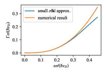
Figure 6: The dependence of the scattering rate $\Gamma$ on the variance of the disorder potential $s$, both in units of $v_{D}/\sigma$, evaluated for average chemical potential $\mu_{0}=0$. Approximation for small impurity potential fluctuations given by Eq. (10) (blue curve) and the true dependence evaluated by means of numerical integration (orange curve).

For larger fluctuations $\delta\mu$ and for $\mu_{0}\neq 0$ the approximation expressed in (10) and (22) and is insufficient. To describe these cases we evaluate the integral exactly

$$\frac{1}{\tau_{\mathbf{k}}}=\frac{2\pi^{2}}{\hbar}\frac{|\mu_{0}|}{\hbar^{2}v_{D}^{2}}\frac{V_{0}^{2}}{\mathcal{N}}\rho_{\mathrm{imp}}\sigma^{4}\exp\left(-2\frac{\mu_{0}^{2}\sigma^{2}}{\hbar^{2}v_{D}^{2}}\right)\\ \left[I_{0}\left(2\frac{\mu_{0}^{2}\sigma^{2}}{\hbar^{2}v_{D}^{2}}\right)+I_{1}\left(2\frac{\mu_{0}^{2}\sigma^{2}}{\hbar^{2}v_{D}^{2}}\right)\right],$$ (27)

where $I_{\alpha}(x)$ are modified Bessel functions of the first kind. Then, we substitute $\mu_{0}\rightarrow\mu_{0}+\delta\mu$ and calculate numerically averages of $1/\tau_{\mathbf{k}}$ with respect to the probability distribution (23). The scattering rate obtained in this way is compared to the approximate formula (10) in Fig. 6, for the special case of $\mu_{0}=0$.

References

- Kitaev (2001) A. Y. Kitaev, Phys. Usp. 44, 131 (2001), arXiv:cond-mat/0010440 [cond-mat.mes-hall] .
- Nayak et al. (2008) C. Nayak, S. H. Simon, A. Stern, M. Freedman, and S. Das Sarma, Rev. Mod. Phys. 80, 1083 (2008), arXiv:0707.1889 [cond-mat.str-el] .
- Alicea (2012) J. Alicea, Rep. Prog. Phys. 75, 076501 (2012), arXiv:1202.1293 [cond-mat.supr-con] .
- Røising et al. (2019) H. S. Røising, R. Ilan, T. Meng, S. H. Simon, and F. Flicker, SciPost Phys. 6, 055 (2019).
- Sarma et al. (2015) S. D. Sarma, M. Freedman, and C. Nayak, npj Quantum Information 1, 15001 (2015).
- Akhmerov (2010) A. R. Akhmerov, Phys. Rev. B 82, 020509 (2010), arXiv:1004.5533 [cond-mat.supr-con] .
- Lutchyn et al. (2010) R. M. Lutchyn, J. D. Sau, and S. Das Sarma, Phys. Rev. Lett. 105, 077001 (2010), arXiv:1002.4033 [cond-mat.supr-con] .
- Oreg et al. (2010) Y. Oreg, G. Refael, and F. von Oppen, Phys. Rev. Lett. 105, 177002 (2010), arXiv:1003.1145 [cond-mat.mes-hall] .
- Lutchyn et al. (2018) R. M. Lutchyn, E. P. a. M. Bakkers, L. P. Kouwenhoven, P. Krogstrup, C. M. Marcus, and Y. Oreg, Nat. Rev. Mater. 3, 52 (2018), arXiv:1707.04899 [cond-mat.supr-con] .
- Aghaee et al. (2023) M. Aghaee, A. Akkala, Z. Alam, R. Ali, A. Alcaraz Ramirez, M. Andrzejczuk, A. E. Antipov, P. Aseev, M. Astafev, B. Bauer, J. Becker, S. Boddapati, F. Boekhout, J. Bommer, T. Bosma, L. Bourdet, S. Boutin, P. Caroff, L. Casparis, M. Cassidy, S. Chatoor, A. W. Christensen, N. Clay, W. S. Cole, F. Corsetti, A. Cui, P. Dalampiras, A. Dokania, G. de Lange, M. de Moor, J. C. Estrada Saldaña, S. Fallahi, Z. H. Fathabad, J. Gamble, G. Gardner, D. Govender, F. Griggio, R. Grigoryan, S. Gronin, J. Gukelberger, E. B. Hansen, S. Heedt, J. Herranz Zamorano, S. Ho, U. L. Holgaard, H. Ingerslev, L. Johansson, J. Jones, R. Kallaher, F. Karimi, T. Karzig, C. King, M. E. Kloster, C. Knapp, D. Kocon, J. Koski, P. Kostamo, P. Krogstrup, M. Kumar, T. Laeven, T. Larsen, K. Li, T. Lindemann, J. Love, R. Lutchyn, M. H. Madsen, M. Manfra, S. Markussen, E. Martinez, R. McNeil, E. Memisevic, T. Morgan, A. Mullally, C. Nayak, J. Nielsen, W. H. P. Nielsen, B. Nijholt, A. Nurmohamed, E. O’Farrell, K. Otani, S. Pauka, K. Petersson, L. Petit, D. I. Pikulin, F. Preiss, M. Quintero-Perez, M. Rajpalke, K. Rasmussen, D. Razmadze, O. Reentila, D. Reilly, R. Rouse, I. Sadovskyy, L. Sainiemi, S. Schreppler, V. Sidorkin, A. Singh, S. Singh, S. Sinha, P. Sohr, T. c. v. Stankevič, L. Stek, H. Suominen, J. Suter, V. Svidenko, S. Teicher, M. Temuerhan, N. Thiyagarajah, R. Tholapi, M. Thomas, E. Toomey, S. Upadhyay, I. Urban, S. Vaitiekėnas, K. Van Hoogdalem, D. Van Woerkom, D. V. Viazmitinov, D. Vogel, S. Waddy, J. Watson, J. Weston, G. W. Winkler, C. K. Yang, S. Yau, D. Yi, E. Yucelen, A. Webster, R. Zeisel, and R. Zhao (Microsoft Quantum), Phys. Rev. B 107, 245423 (2023), arXiv:2207.02472 [cond-mat.mes-hall] .
- Fu and Kane (2008) L. Fu and C. L. Kane, Phys. Rev. Lett. 100, 096407 (2008), arXiv:0707.1692 [cond-mat.mes-hall] .
- Jauregui et al. (2018) L. A. Jauregui, M. Kayyalha, A. Kazakov, I. Miotkowski, L. P. Rokhinson, and Y. P. Chen, Applied Physics Letters 112, 093105 (2018), arXiv:1710.03362 [cond-mat.mes-hall] .
- Rosen et al. (2021) I. T. Rosen, C. J. Trimble, M. P. Andersen, E. Mikheev, Y. Li, Y. Liu, L. Tai, P. Zhang, K. L. Wang, Y. Cui, M. A. Kastner, J. R. Williams, and D. Goldhaber-Gordon, “Fractional AC Josephson effect in a topological insulator proximitized by a self-formed superconductor,” (2021), arXiv:2110.01039 [cond-mat.mes-hall] .
- Rüßmann and Blügel (2022) P. Rüßmann and S. Blügel, “Proximity induced superconductivity in a topological insulator,” (2022), arXiv:2208.14289 [cond-mat.mes-hall] .
- Kong et al. (2019) L. Kong, S. Zhu, M. Papaj, H. Chen, L. Cao, H. Isobe, Y. Xing, W. Liu, D. Wang, P. Fan, Y. Sun, S. Du, J. Schneeloch, R. Zhong, G. Gu, L. Fu, H.-J. Gao, and H. Ding, Nature Physics 15, 1181 (2019), arXiv:1901.02293 [cond-mat.supr-con] .
- Chiu et al. (2020) C.-K. Chiu, T. Machida, Y. Huang, T. Hanaguri, and F.-C. Zhang, Science Advances 6, eaay0443 (2020), arXiv:1904.13374 [cond-mat.supr-con] .
- Xu et al. (2015) J.-P. Xu, M.-X. Wang, Z. L. Liu, J.-F. Ge, X. Yang, C. Liu, Z. A. Xu, D. Guan, C. L. Gao, D. Qian, Y. Liu, Q.-H. Wang, F.-C. Zhang, Q.-K. Xue, and J.-F. Jia, Phys. Rev. Lett. 114, 017001 (2015), arXiv:1312.7110 [cond-mat.supr-con] .
- Sun et al. (2016) H.-H. Sun, K.-W. Zhang, L.-H. Hu, C. Li, G.-Y. Wang, H.-Y. Ma, Z.-A. Xu, C.-L. Gao, D.-D. Guan, Y.-Y. Li, C. Liu, D. Qian, Y. Zhou, L. Fu, S.-C. Li, F.-C. Zhang, and J.-F. Jia, Phys. Rev. Lett. 116, 257003 (2016), arXiv:1603.02549 [cond-mat.supr-con] .
- Lee (2020) J. U. Lee, “Scalable gate-defined Majorana fermions in 2D p-wave superconductors,” (2020), arXiv:2011.08925 [cond-mat.mes-hall] .
- Akzyanov et al. (2014) R. S. Akzyanov, A. V. Rozhkov, A. L. Rakhmanov, and F. Nori, Phys. Rev. B 89, 085409 (2014), arXiv:1307.0923 [cond-mat.str-el] .
- Deng et al. (2020) H. Deng, N. Bonesteel, and P. Schlottmann, Journal of Physics: Condensed Matter 33, 035604 (2020), arXiv:2001.03666 [cond-mat.supr-con] .
- Ziesen and Hassler (2021) A. Ziesen and F. Hassler, Journal of Physics Condensed Matter 33, 294001 (2021), arXiv:2101.06208 [cond-mat.supr-con] .
- Ioselevich et al. (2012) P. A. Ioselevich, P. M. Ostrovsky, and M. V. Feigel’man, Phys. Rev. B 86, 035441 (2012), arXiv:1205.4193 [cond-mat.mes-hall] .
- Ziesen et al. (2023) A. Ziesen, A. Altland, R. Egger, and F. Hassler, Phys. Rev. Lett. 130, 106001 (2023), arXiv:2211.15296 [cond-mat.mes-hall] .
- Pikulin and Franz (2017) D. I. Pikulin and M. Franz, Phys. Rev. X 7, 031006 (2017), arXiv:1702.04426 [cond-mat.dis-nn] .
- Marchand and Franz (2012) D. J. J. Marchand and M. Franz, Phys. Rev. B 86, 155146 (2012), arXiv:1209.4055 [cond-mat.str-el] .
- Note (1) The decay length of the wave functions in the SC is given by .
- Xu et al. (2014) Y. Xu, I. Miotkowski, C. Liu, J. Tian, H. Nam, N. Alidoust, J. Hu, C.-K. Shih, M. Z. Hasan, and Y. P. Chen, Nature Physics 10, 956 (2014), arXiv:1409.3778 [cond-mat.mes-hall] .