A Database of Magnetic and Thermodynamic Properties of Confined And Eruptive Solar Flares

Abstract

Solar flares sometimes lead to coronal mass ejections that directly affect the Earth’s environment. However, a large fraction of flares, including on solar-type stars, are confined flares. What are the differences in physical properties between confined and eruptive flares? For the first time, we quantify thermodynamic and magnetic properties of hundreds of confined and eruptive flares of GOES class C5.0 and above, $480$ flares total. We first analyze large flares of GOES class M1.0 and above observed by the Solar Dynamics Observatory (SDO): $216$ flares total, including $103$ eruptive and $113$ confined flares, from 2010 until 2016 April, we then look at the entire dataset above C5.0 of $480$ flares. We compare GOES X-ray thermodynamic flare properties, including peak temperature and emission measure, and active-region and flare-ribbon magnetic field properties, including reconnected magnetic flux and peak reconnection rate. We find that for fixed peak X-ray flux, confined and eruptive flares have similar reconnection fluxes; however, for fixed peak X-ray flux confined flares have on average larger peak magnetic reconnection rates, are more compact, and occur in larger active regions than eruptive flares. These findings suggest that confined flares are caused by reconnection between more compact, stronger, lower lying magnetic-fields in larger active regions that reorganizes smaller fraction of these regions’ fields. This reconnection proceeds at faster rates and ends earlier, potentially leading to more efficient flare particle acceleration in confined flares.

1 Introduction

Flares are classified into eruptive and confined types according to their association with coronal mass ejections (CMEs, Moore et al. 2001; Wang & Zhang 2007; Thalmann et al. 2015; Temmer 2021; Afanasyev et al. 2023). In an eruptive flare, plasma is ejected into interplanetary space and is later observed as a CME in white-light coronagraph images, although its visibility might greatly depend on flare intensity (Yashiro et al., 2006). In a non-eruptive (or confined or compact) flare, plasma falls back to the Sun and there is no CME. On the Sun both types of flares are frequent: for example, from 2010 to 2019 only half of large solar flares of GOES class M1.0 and above flares were eruptive and led to CMEs; another half were confined flares (Li et al., 2020). On solar-type cool stars, up to now there have been only $40$ CME detections (Moschou et al., 2019; Veronig et al., 2021; Namekata et al., 2022).

While comparison of confined and eruptive flares on solar-like stars is difficult due to lack of spatial resolution, on the Sun we can measure both magnetic and thermodynamics properties of flares in high detail (see Figure 1). With the launch of the Solar Dynamics Observatory in 2010, the number of studies comparing properties of eruptive and confined flares surged. For example, Cheng et al. (2011) analyzed $9$ M- and X-class flares all from the same active region (AR) to understand magnetic and thermodynamic properties of $6$ confined and $3$ eruptive events. Harra et al. (2016) analyzed properties of $9$ confined and $33$ eruptive flares, $42$ X-class flares total. Hinterreiter et al. 2018 and Tschernitz et al. (2018) analyzed $50$ flares, $19$ eruptive and $31$ confined events, C-class and above. Toriumi et al. (2017) surveyed $51$ flares, $32$ eruptive and $19$ confined events, M5.0-class and above. Finally, Li et al. (2020) analyzed $322$ flares, $170$ eruptive and $152$ confined events, M1.0-class and above, followed by the largest-to-date study, by Li et al. (2021), of $719$ flares, $251$ eruptive and $468$ confined events, C5.0-class and above.

Two physical concepts are typically used to describe whether a flare would be eruptive or confined. The first factor describes the degree of AR non-potentiality, i.e. magnetic free energy, twist, helicity, etc. The second factor describes the constraining effect of the strapping or overlying field: its strength and decay rate with height. The torus instability occurs once the decay index of $n=-\frac{\partial\mathrm{ln}{B}_{\mathrm{p}}}{\partial\mathrm{ln}z}$ for poloidal field ${B}_{\mathrm{p}}$ reaches a critical eruptive value of $n_{\mathrm{cr}}$ at a critical height $h_{\mathrm{cr}}$. In this case the poloidal component refers to the component of the strapping field perpendicular to the axis of the toroidal flux rope. For critical values, a range within $0.5$ to $2$ is typically used, depending on the magnetic configuration (see e.g., Török & Kliem 2005; Kliem & Török 2006; Wang & Zhang 2007; Myers et al. 2015; Sun et al. 2015, 2022; Hassanin & Kliem 2016; Hassanin et al. 2022 and references therein). In particular, a value of $n_{c}=1.5$ for a thin, axisymmetric torus (Bateman, 1978) is widely used in observational studies. As larger total unsigned AR magnetic flux leads to increased critical decay-index height $h_{\mathrm{cr}}$, ARs with large magnetic flux have confined eruptions due to strong magnetic cages (e.g., Amari et al. 2018; Li et al. 2021).

Below we review some magnetic field properties quantified in confined and eruptive events from observations. For more details on recent statistical studies of flare magnetic properties, we recommend reading our recent review paper (Kazachenko et al., 2022a).

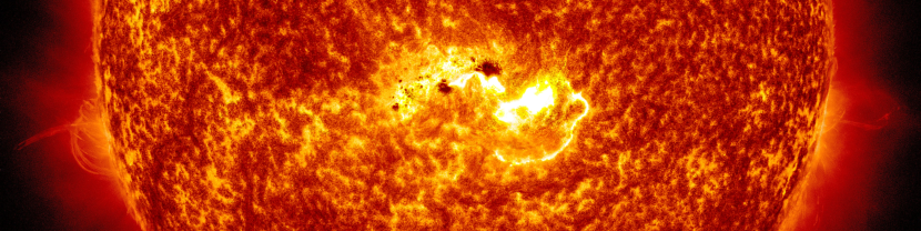
Figure 1: X1.2-class eruptive solar flare observed by the Solar Dynamics Observatory in 1600Å and 304Å wavelengths. Bright ribbons mark the footpoints of reconnected fields lines thaft provide indirect measurement of the amount of reconnecting magnetic flux in the flare and the reconnection rate.

The main magnetic-field properties typically used to distinguish confined from eruptive events include total unsigned magnetic fluxes of flare-hosting ARs, $\Phi_{\mathrm{AR}}$ (Li et al., 2021), fractions of the active-region magnetic flux or area swept by flare ribbons, $\Phi_{\mathrm{rbn}}$ and $S_{\mathrm{rbn}}$, relative to the total AR flux or area, $R_{\Phi}=\Phi_{\mathrm{rbn}}/\Phi_{\mathrm{AR}}$ and $R_{S}=S_{\mathrm{rbn}}/S_{\mathrm{AR}}$, respectively (Thalmann et al., 2015; Masson et al., 2017; Tschernitz et al., 2018; Toriumi et al., 2017; Li et al., 2020; Kazachenko et al., 2022b), and the ratio of the twist near the flaring polarity inversion line (PIL) to the AR magnetic flux, $\alpha_{\mathrm{PIL}}/\Phi_{\mathrm{AR}}$ (relative non-potentiality, Li et al. 2022). For a given flare class, eruptive flares involve larger fraction of AR magnetic flux and area, tend to occur in smaller ARs and have a larger ratio of the twist near the PIL to the AR flux. Using a sample of $43$ eruptive and $63$ confined flares, Li et al. (2022) found that the relative non-potentiality parameter of $\alpha_{\mathrm{PIL}}/\Phi_{\mathrm{AR}}>2.2\times 10^{-24}Mm^{-1}Mx^{-1}$ distinguishes about $93\%$ of eruptive events. On the other hand, confined flares have smaller fractions of AR magnetic flux and area, tend to occur in larger ARs and have a smaller ratio of the twist near the PIL to the AR flux. Again, in the work by Li et al. (2022) the above relative non-potentiality of $\alpha_{\mathrm{PIL}}/\Phi_{\mathrm{AR}}<2.2\times 10^{-24}Mm^{-1}Mx^{-1}$ distinguishes about $83\%$ of confined events. In addition, from analysis of photospheric vector magnetic fields, Liu et al. (2017); Vemareddy (2019); Avallone & Sun (2020), and Kazachenko et al. (2022b) found that confined flares tend to occur in ARs that are more current-neutralized, and have a smaller amount of magnetic shear at the PIL. As shear and net current are proportional to each other through Ampere’s law, smaller shear and net current in confined flares both support the same physical concept of smaller magnetic-field non-potentiality at the PIL (Kazachenko et al., 2022b). To summarize, existing analyses of magnetic field observations fit within the above scenario that smaller non-potentiality and stronger overlying fields in confined flares constrain plasma from escaping. In terms of magnetic topology of pre-flare magnetic field, both confined and eruptive flares could originate from a sheared arcade or a flux rope (Masson et al., 2017) with one or several confined flares preceding an eruption (Kliem et al., 2021; Hassanin et al., 2022).

Numerous studies found that proximity of the flaring part of the AR to the AR boundary and the open field affect the flare eruptivity. For example, Tschernitz et al. (2018) found that for a given X-ray flux, confined events tend to have larger mean magnetic-flux density, implying that they tend to occur closer to the center of ARs where fields are stronger. Cheng et al. (2011) came to a similar conclusion, finding that confined flares occur closer to AR centers than eruptive flares, in agreement with Wang & Zhang (2007). Using non-linear force-free field extrapolation, they also found that in the low corona ($\approx 10$ Mm), eruptive flares have a higher decay index of the transverse magnetic field than confined flares. In addition, the strength of the transverse magnetic field over the eruptive flare sites is weaker than it is over the confined ones in agreement with e.g., Cui et al. (2018); Vasantharaju et al. (2018). Finally, Derosa & Barnes (2018) analyzed the PFSS global magnetic fields. Using a sample of $50$ eruptive and $6$ confined flares, they found that confined events have slightly less access to open flux than eruptive events. However this difference is not large: the rate at which X-class flares are eruptive is $0.97$ (30 out of 31 flares) and $0.8$ ($20/25$) for events with and without access to open flux, respectively. This result agrees with Baumgartner et al. (2018). In addition, an active region could become more prone to host a confined flare when the orientation between its local and overlying magnetic flux systems becomes less antiparallel (Zuccarello et al., 2017).

Among other properties differing in confined and eruptive flares, average ribbon-separation distances and ribbon-peak separation speeds tend to be smaller for confined flares (Kurokawa, 1989; Su et al., 2007; Veronig & Polanec, 2015; Thalmann et al., 2015; Hinterreiter et al., 2018). One explanation for this could be strong overlying fields in confined events which prevent reconnecting current sheet from moving upwards. As ribbon separation speed is a proxy for a localized reconnection rate, results by Hinterreiter et al. (2018); Thalmann et al. (2015) imply that eruptive flares might have higher local reconnection rate, however the authors of these papers do not explicitly state this. Note also, that while Hinterreiter et al. (2018) analyzed a large number of flares of different flare classes ($50$ flares, $31$ confined and $19$ eruptive), ranging from B- to X-class, their distributions of GOES peak X-ray fluxes of confined and eruptive flare samples were different, with the confined flare sample being significantly smaller than eruptive sample.

While a large number of statistical studies compared confined and eruptive flares’ magnetic properties, few have analyzed thermodynamic properties and energy partition of confined flares and even fewer have compared those with eruptive events. Kahler & Ling (2022) analyzed GOES peak temperatures in hundreds of flares, of flare class M3.0 and above, and found, that for a given peak X-ray flux, confined flares have higher temperatures than eruptive flares, confirming earlier results of Kay et al. (2003) study of $69$ flares. Cheng et al. (2011) analyzed $9$ M- and X-class flares from the same ARs: $6$ confined and $3$ eruptive events. They found that confined flares have more impulsive soft X-ray time profiles, while eruptive flare have longer durations and extend over larger areas in EUV 195 Å images. Harra et al. (2016) analyzed $42$ flares, X-class and above: $9$ confined and $33$ eruptive flares. For their sample they found no statistical differences in thermal and magnetic properties between confined and eruptive flares. Tan et al. (2021) analyzed radio and X-ray data from GOES, RHESSI, and Fermi/GBM from 10 mostly confined flares in AR 12192. They found that the magnetic field in confined flares tends to be stronger than that in $412$ eruptive flares studied by Nita et al. 2004. They also found that confined flares are efficient particle accelerators, however the energies to which electrons are accelerated in confined flares are lower (and do not produce HXR above $300$ keV, indicating the lack of efficient acceleration of electrons to high energies), in agreement with Thalmann et al. (2015). Cai et al. (2021) analyzed energy partition in $4$ confined flares. They found that the ratio of non-thermal energies to magnetic energies is significantly larger for confined than for eruptive flares, ranging within $E_{\mathrm{nth}}/E_{\mathrm{mag}}\approx 0.7-0.76$, in agreement with case study by Thalmann et al. (2015). This implies that larger fraction of free energy is converted into kinetic energy of flare-accelerated electrons in confined flares, while a larger fraction of free energy is converted into other forms of energy, such as kinetic energy of particles, thermal energy, and CME kinetic energy, in eruptive flares (Emslie et al., 2005; Reeves et al., 2010; Emslie et al., 2012; Warmuth & Mann, 2016; Aschwanden et al., 2015, 2017). Given that CME kinetic energy is the largest fraction in the eruptive-flare energy partition, it is not surprising that eruptive flares have smaller energy fractions in accelerated particles, compared with confined flares. Finally, Qiu & Cheng (2022) analyzed three eruptive (M2.0, M6.9 and M1.5) and three confined (C8.2, C8.7 and C9.8) flares. They found that in eruptive flares non-thermal HXR emission lags the EUV emission from flare ribbons, suggesting that eruptive flares have a gradual warm-up phase with lower non-thermal energy release efficiency. They also found that, on average, confined flares exhibit stronger magnetic shear and high-temperature component (up to $25$ MK for up to one minute) at the onset, which is not present in eruptive flares (in agreement with case study by Veronig & Polanec 2015). Note, however, that eruptive flares in the study by Qiu & Cheng (2022) had larger flare classes than confined events; ideally, flare samples of similar flare classes should be compared. To summarize, confined flares are efficient particle accelerators located lower in the corona in agreement with earlier studies (e.g., Klein et al. 2010), with only a small fraction of particles accelerated to extremely high energies.

While most statistical papers focused on magnetic properties of eruptive/confined flares and few analyzed their thermodynamic properties, in this paper our goal is to fill this gap to create a comprehensive survey of both thermodynamic and magnetic properties of eruptive and confined flares on the Sun for a large, balanced sample. For this, we analyze properties of all flares of GOES class C5.0 and above observed by the SDO from 2010 to 2016 within $45^{\circ}$ from the central meridian. To minimize errors in the reconnection fluxes we restrict our analysis to events with reconnection flux imbalance between positive and negative polarities $\Phi_{\mathrm{ribbon,imb}}<20\%$. As a result we select $480$ events total: $152$ eruptive and $328$ confined flares of GOES class C5.0 and above. Since the number of confined and eruptive flares in this sample is highly unbalanced, we first analyze a more balanced subsample of large flares of GOES class M1.0 and above, $216$ events total: $103$ eruptive and $113$ confined flares. We then present an analysis for the whole dataset, coming to similar physical conclusions (see Appendix A). We analyze the following flare properties: AR magnetic fluxes, magnetic-reconnection fluxes and their peak rates, flare thermodynamic properties (temperature, emission measure) and flare durations.

This paper is organized as follows. In Section 2, we describe the four datasets that we use to assemble our final dataset, the variables and the procedures to evaluate uncertainties. In Section 3 we discuss our results for $216$ flares of GOES class M1.0 and above. For comparison, in Appendix A we present results for a larger sample of $480$ flares that includes smaller flares above C5.0. Finally, in Section 4, we summarize our conclusions for both flare samples.

2 Data and Methodology

Table 1 shows a list of physical properties and their data source that we use for each flare in our analysis. These properties include flare location, GOES peak X-ray flux, GOES time-integrated flux (fluence), GOES start, peak, end times and durations; GOES peak temperature and emission measure; AR area and unsigned magnetic flux; unsigned reconnection flux, peak reconnection rate, ribbon area and eruptivity (confined or eruptive) of each flare.

For initial flare detections and estimates of flare reconnection flux, ribbon area and their uncertainties we use RibbonDB dataset (Kazachenko et al., 2017). RibbonDB database contains 3137 solar flare ribbon events corresponding to every flare of GOES class C1.0 and greater within $45^{\circ}$ of the central meridian, from 2010 April until 2016 April, observed by the Atmospheric Imaging Assembly (AIA, Lemen et al. 2012) on board the SDO in 1600Å (see Eq. 7-11 in Kazachenko et al. 2017). To remind the reader, we sum up flux of positive and negative magnetic polarities within flare ribbons to find the unsigned ribbon reconnection flux (or AR unsigned flux):

$$\Phi_{\mathrm{ribbon}}=\Phi^{+}_{\mathrm{ribbon}}+\Phi^{-}_{\mathrm{ribbon}}=\frac{\Phi^{\mathrm{+(I_{6})}}+\Phi^{\mathrm{+(I_{10})}}}{2}+\frac{\Phi^{\mathrm{-(I_{6})}}+\Phi^{\mathrm{-(I_{10})}}}{2}=\frac{\Phi^{\mathrm{(I_{6})}}+\Phi^{\mathrm{(I_{10})}}}{2},$$ (1)

where $|\Phi^{+}_{\mathrm{ribbon}}|$ and $|\Phi^{-}_{\mathrm{ribbon}}|$ are signed reconnection fluxes in each polarity. Above, we take an average between ribbon fluxes in areas with $c=6$ and $c=10$ times the median background intensity for the minimum ribbon brightness. We do this to account for the uncertainty in ribbon edge identification due to variable choice of background cutoff (see Equations (5) and (6) in Kazachenko et al. 2017):

$$\Phi^{\mathrm{\pm(I_{c})}}_{\mathrm{ribbon}}=\int_{I_{c},(>or<100G)}|B_{n}|dS.$$ (2)

The error in the unsigned reconnection flux (or the ribbon area) is then

$$\Delta\Phi_{\mathrm{ribbon}}=\frac{\Phi^{\mathrm{(I_{6})}}-\Phi^{\mathrm{(I_{10})}}}{2}.$$ (3)

Following Kazachenko et al. (2017), we define percentages of the ribbon-to-AR magnetic fluxes and ribbon-to-AR areas, respectively, as

$$R_{\Phi}=\frac{\Phi_{\mathrm{ribbon}}}{\Phi_{\mathrm{AR}}}\times 100\%,\;\;\;\;\;R_{S}=\frac{S_{\mathrm{ribbon}}}{S_{\mathrm{AR}}}\times 100\%.$$ (4)

We also find mean magnetic flux density within AR and ribbon areas as $\bar{B}_{\mathrm{AR}}=\frac{\Phi_{\mathrm{AR}}}{S_{\mathrm{AR}}}$ and $\bar{B}_{\mathrm{ribbon}}=\frac{\Phi_{\mathrm{ribbon}}}{S_{\mathrm{ribbon}}}$, respectively.

Table 1: List of variables we analyzed for 216 $>$M1.0-class flares and 480 $>$C5.0-class flares (see Appendix A) and reference to their data source: RibbonDB (Kazachenko et al., 2017), Plutino et al. (2023), TEBBS (Sadykov et al., 2019) and Li et al. (2021). The data is available online.

Variable	Description	Units	Data Source Reference
$I_{\rm X,peak}$	Peak 1-8Å X-ray flux, GOES	[W m-2]	Plutino et al. (2023)
$t_{\rm start}$	Flare start time	[UT]	Plutino et al. (2023)
$t_{\rm peak}$	Flare peak time	[UT]	Plutino et al. (2023)
$t_{\rm end}$	Flare end time	[UT]	Plutino et al. (2023)
$\tau=t_{\rm end}-t_{\rm start}$	Flare duration	[min]	Plutino et al. (2023)
$\tau_{\mathrm{rise}}=t_{\rm peak}-t_{\rm start}$	Flare duration (rise)	[min]	Plutino et al. (2023)
$F_{\mathrm{X}}$	X-ray total flux (fluence)	[W m${}^{-2}s$]	Plutino et al. (2023)
$T_{\rm GOES}$	Flare peak temperature, GOES	[MK]	TEBBS
$EM_{\rm GOES}$	Flare peak EM, GOES	[$10^{48}cm^{-3}$]	TEBBS
$lon,lat$	Flare longitude and latitude	[deg]	RibbonDB
$AR_{\rm number}$	AR NOAA number	$-$	RibbonDB
$\Phi_{AR}$	Unsigned AR flux	[Mx]	RibbonDB
$\Phi_{\mathrm{ribbon}}$	Unsigned reconnection flux	[Mx]	RibbonDB
$\Delta\Phi_{\rm ribbon}$	Uncertainty in $\Phi_{\mathrm{ribbon}}$	[Mx]	RibbonDB
$\Phi_{\rm ribbon,imb}$	Imbalance in $\Phi_{\mathrm{ribbon}}$	[Mx]	RibbonDB
$\dot{\Phi}_{\rm ribbon}$	Peak reconnection flux rate	[Mx/s]	RibbonDB
$\Delta\dot{\Phi}_{\rm ribbon}$	Uncertainty in $\dot{\Phi}_{\rm ribbon,peak}$	[Mx/s]	RibbonDB
$\dot{\Phi}_{\rm ribbon,imb}$	Imbalance in $\dot{\Phi}_{\rm ribbon,peak}$	[Mx/s]	RibbonDB
$S_{\mathrm{AR}}$	AR area	[cm2]	RibbonDB
$S_{\mathrm{ribbon}}$	Ribbon area	[cm2]	RibbonDB
$\Delta S_{\rm ribbon}$	Uncertainty in $S_{\mathrm{ribbon}}$	[cm2]	RibbonDB
$R_{\Phi}$	Reconnection flux fraction	[%]	RibbonDB
$R_{S}$	Ribbon area fraction	[%]	RibbonDB
$\epsilon$	Eruptivity: 1 - eruptive, 0 - confined	$-$	Li et al. (2021)

^a http://solarmuri.ssl.berkeley.edu/~kazachenko/SolarErupDB/

We further expand the original RibbonDB dataset to include peak reconnection flux rate $\dot{\Phi}_{\rm ribbon,peak}$ and imbalances in reconnection flux and the peak reconnection flux rate, $\Phi_{\rm ribbon,imb}$ and $\dot{\Phi}_{\rm ribbon,imb}$. Peak reconnection flux rate here describes the global peak rate of magnetic reconnection flux over the whole active region. The imbalance is the difference between positive and negative magnetic polarities $\Phi_{\mathrm{imb}}=\left|~{}|\Phi_{\mathrm{+}}|-|\Phi_{\mathrm{+}}|~{}\right|$ and should ideally be equal to zero for an isolated well-observed AR or a set of footpoints brightened by the flare ribbons. Therefore we use this quantity as an additional quality-control measure for our magnetic fluxes. Specifically, we define the imbalance in the reconnection flux as

$$\Phi_{\mathrm{ribbon,imb}}=\left|~{}|\Phi^{+}_{\mathrm{ribbon}}|-|\Phi^{-}_{\mathrm{ribbon}}|~{}\right|.$$ (5)

Similarly, we define imbalance in the peak reconnection flux rate as

$$\dot{\Phi}_{\mathrm{ribbon,imb}}=\left|~{}|\dot{\Phi}^{+}_{\mathrm{ribbon}}|-|\dot{\Phi}^{-}_{\mathrm{ribbon}}|~{}\right|,$$ (6)

where positive and negative values are signed peak reconnection rates in each polarity. To minimize errors in the reconnection fluxes we restrict our analysis to events with reconnection flux imbalance between positive and negative polarities $\Phi_{\mathrm{ribbon,imb}}<20\%$.

How suitable are ribbon reconnection flux and peak reconnection rate for description of release of magnetic energy in solar flares? As footpoints of reconnected fields, flare ribbons only identify magnetic fields participating in the flare reconnection. However, they do not directly capture dynamics of arcades adjacent or below reconnected fields that evolve as part of the overall relaxation of the coronal field (Hudson, 2000; Wang et al., 2018; Yadav & Kazachenko, 2023). What is the energetic significance of changes in fields that do not directly participate in the reconnection process? From comparison of magnetic energy released in the reconnection process and CMEs’ energies (summed kinetic and gravitational potential energies), Zhu et al. (2020) found that for large M- and X-class flares reconnection dominates CME acceleration in fast CMEs, in agreement with earlier works by Longcope et al. (2007); Kazachenko et al. (2012). However, for smaller B- and C-class flares, work done by the reconnection electric field in the current sheet itself might not be enough to fuel the eruption. Furthermore, there is a strong correlation between the reconnection flux and the GOES peak X-ray flux ($r_{s}=[0.6-0.9]$, Sindhuja & Gopalswamy 2020; Toriumi et al. 2017; Kazachenko et al. 2017; Tschernitz et al. 2018; Kazachenko et al. 2022a). Based on these arguments, we assume that it is reasonable to expect that the total amount of energy released in an event scales with magnetic reconnection flux and reconnection rate, recognizing that these observables capture the key aspects of the relaxation process.

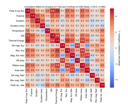
Figure 7: Appendix: Correlation matrix showing Spearman correlation coefficient between different physical variables for all flares with GOES flare class $>C5.0$. See Appendix A for details.

To find the flare GOES peak X-ray flux and fluence, and also flare start, peak and end times, $I_{\mathrm{X,peak}},F_{\mathrm{X}},t_{\mathrm{start}},t_{\mathrm{peak}},t_{\mathrm{end}}$, we use a database by Plutino et al. (2023). In contrast to Heliophysics Event Catalog (HEC) that we used in RibbonDB catalog to identify flare peak X-ray flux, start, peak and end times, Plutino et al. (2023) catalog uses a method by Aschwanden & Freeland (2012) to identify flares in the GOES SXR light curve. As a result, the catalog of Plutino et al. (2023) has slightly different values for peak X-ray fluxes and also flare times, compared to RibbonDB (see Figure 7 in Plutino et al. 2023). For flare total and rise time durations we use

$$\tau=t_{\mathrm{end}}-t_{\mathrm{start}}\;\;\;\;\;and\;\;\;\;\;\tau_{\mathrm{rise}}=t_{\mathrm{peak}}-t_{\mathrm{start}},$$ (7)

respectively. In our analysis, we only used RibbonDB flare peak X-ray fluxes for initial selection of events.

To find the GOES peak temperature $T_{\mathrm{GOES}}$ and emission measure $EM_{\mathrm{GOES}}$, we use Temperature and EM-Based Background Subtraction algorithm (TEBBS) dataset from Sadykov et al. (2019), deduced from GOES SXR observations. In the TEBBS dataset Sadykov et al. (2019) apply TEBBS algorithm (Bornmann, 1990; Ryan et al., 2012) to estimate $T_{\mathrm{GOES}}$ and $EM_{\mathrm{GOES}}$ for all solar flares from 2002 January until 2017 December. $T_{\mathrm{GOES}}$ describes the maximum temperature of the dense chromospheric plasma after the flare starts. $EM_{\mathrm{GOES}}$ describes the maximum emission measure that the chromospheric plasma reaches as it first evaporates and then condenses back into the chromosphere. Note that in this approach, as the GOES data includes only two SXR energy channels, both the flare temperature and EM are calculated in a single-temperature approximation, which is a simplification given evidence for multi-temperature structure (Warmuth & Mann, 2016).

In addition, we use GOES peak temperature $T_{\mathrm{GOES}}$ and emission measure $EM_{\mathrm{GOES}}$ to calculate flare thermal energy at the time of peak temperature, $E_{\mathrm{th,GOES}}=3nk_{B}T_{\mathrm{GOES}}V$. From the emission measure $EM_{\mathrm{GOES}}\approx n^{2}V$, we find density $n=\sqrt{\frac{EM_{\mathrm{GOES}}}{V}}$, where for the flare loop volume $V$ we use $V=(\frac{S_{\mathrm{ribbon}}}{2})^{3/2}$. Then the expression for thermal energy becomes (Reep & Knizhnik, 2019)

$$E_{\mathrm{th,GOES}}=\frac{3}{8^{1/4}}k_{B}(EM_{\mathrm{GOES}})^{1/2}S^{3/4}_{\mathrm{ribbon}}T_{\mathrm{GOES}}.$$ (8)

Finally, to define whether each flare is confined or eruptive, we use the database of Li et al. (2021). This database includes 719 flares ($251$ eruptive and $468$ confined) of GOES class C5.0 and greater that occurred within $45^{\circ}$ of the central meridian, from June 2010 until June 2019. To define flare eruptivity, this dataset uses the CDAW CME catalog (Yashiro et al., 2004) based on the Solar and Heliospheric Observatory/Large Angle and Spectrometric Coronagraph (SOHO/LASCO, Brueckner et al. 1995) observations, data from the twin Solar Terrestrial Relations Observatory (STEREO) and EUV wave detections from the AIA.

Figure 2 shows our final dataset of $480$ flares, $152$ eruptive and $328$ confined, with GOES class C5.0 and above, that we use for analysis of large ($>M1.0$) and all ($>C5.0$) flares. The top panel shows the total number of confined and eruptive flares as a function of time; the bottom panel shows their location on the solar disk grouped by ARs and colored by the cumulative GOES peak X-ray class. As the fraction of confined flares increases for smaller GOES peak X-ray class, we intentionally limit our first study to flares above M1.0, which includes a roughly equal number of confined and eruptive flares: $103$ eruptive and $113$ confined flares. This list corresponds to all flares of GOES class M1.0 and above observed by SDO from $2010$ to $2016$ April within $45^{\circ}$ of the central meridian, spanning the majority of solar cycle $24$. In this final dataset we determine flare GOES X-ray properties using the dataset of Plutino et al. (2023) dataset, flare ribbon properties from the RibbonDB dataset (Kazachenko et al., 2017), flare thermodynamic properties using the TEBBS dataset (Sadykov et al., 2019) and flare eruptivity using Li et al. (2021) list.

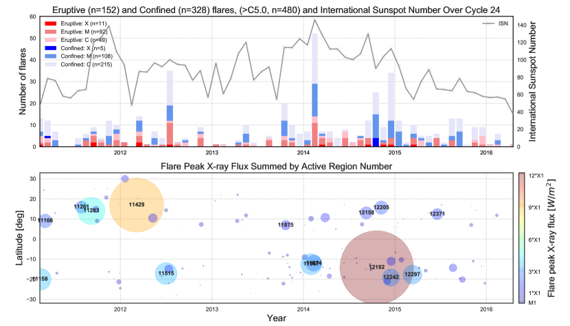
Figure 2: Our dataset of $480$ flares ($152$ eruptive and $328$ confined flares), including $103$ eruptive and $113$ confined M- and X-class flares (see §3) and $49$ eruptive and $215$ confined C-class flares (see Appendix A). Top panel: number of confined and eruptive C-, M- and X-class flares each month analyzed in this paper (left axis) and sunspot number from 2010 April until 2016 April (right axis). These flares correspond to all events above C5.0 from the flare ribbon database RibbondDB. Bottom panel: flare peak X-ray flux and latitude grouped by AR vs. time; circle size and color correspond to the peak X-ray flux summed over each AR number. See §2 for details.

We describe the quantitative relationship between flare and AR properties, e.g., $\mathbb{X}$ and $\mathbb{Y}$, using the Spearman ranking correlation coefficient, $r_{s}(\mathbb{X},\mathbb{Y})$. Specifically for qualitative strength of the correlation $r_{s}$ we use: $r_{s}\in[0.2,0.39]$ – weak, $r_{s}\in[0.4,0.59]$ – moderate, $r_{s}\in[0.6,0.79]$ – strong, and $r_{s}\in[0.8,1.0]$ – very strong.

2.1 Uncertainties

We recognize that the variables we analyze have uncertainties. For example, identification of eruptive/confined flares might be ambiguous due to observational constraints (see e.g., an $M4.0$ flare on 2011 September 26 in AR 11302 that was identified as eruptive in the catalog of Li et al. (2021), but confined by Gupta et al. 2021). As another example, reconnection fluxes in the RibbonDB using 1600 Å SDO images are slightly different from reconnection fluxes evaluated using Kanzelhohe Solar Observatory (KSO) ribbon images in $H_{\alpha}$ and $CaK$ bands (Sindhuja et al., 2019). While we could not re-examine all events, where possible, we evaluated uncertainties without modifying the main quantities. For unsigned reconnection fluxes $\Phi_{\mathrm{ribbon}}$ (Eq. 1), we evaluated errors based on uncertainty in the median background intensity $\Delta\Phi_{\mathrm{ribbon}}$ (Eq. 3). For unsigned peak reconnection fluxes and their rates, we evaluated error proxies based on the imbalance over positive and negative polarities (Eqs. 5 and 6). Furthermore we restrict our analysis to events with reconnection flux imbalance of less than $20\%$. Note that we have not assessed the accuracy of TEBBS estimates for peak temperature and emission measure and confinement/eruptivity detections of Li et al. (2021).

3 Results: Flares of GOES Class M1.0 and Larger

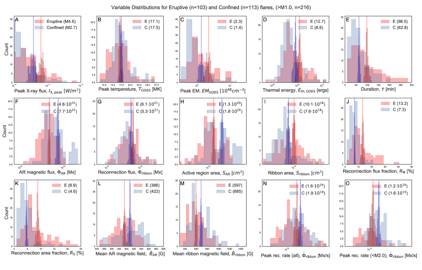
Figure 3: Results: Distributions of various physical variables for eruptive (red) and confined (blue) events ($>M1.0$ GOES flare class). Vertical dotted lines and numbers in the top right corner indicate the mean value for each variable within eruptive and confined flare groups. Darker-color histograms near dotted lines show distributions of the mean, if we select $100$ random subsamples of the half of the events in each sample, and reflect variability of the mean due to event selection. See §3.1 for details.

Table 2: Confined vs. Eruptive flares: comparison of typical ranges and mean values of their magnetic and thermodynamic properties for 216 $>$M1.0-class flares. The typical range of each quantity is described as the $20^{th}$ to $80^{th}$ percentile $\mathbb{X}[P_{20},P_{80}]$. See §3.1 for details and Fig. 3 for distribution plots of all variables.

		CONFINED FLARES		ERUPTIVE FLARES
Quantity	Units	Typical range	Mean Value	Typical range	Mean Value	Figure
$\mathbb{X}$		$\mathbb{X}_{\mathrm{conf}}[P_{20},P_{80}]$	$\bar{\mathbb{X}}_{\mathrm{conf}}$	$\mathbb{X}_{\mathrm{erup}}[P_{20},P_{80}]$	$\bar{\mathbb{X}}_{\mathrm{erup}}$
Peak X-ray flux, $I_{\mathrm{X,peak}}$	Flare class	[M1.4,M4.1]	$M2.7$	$[M1.8,M8.9]$	$M4.6$	Fig. 3(A)
Duration, ${\tau}$	$min$	$[31,91]$	$63$	$[41,148]$	$99$	Fig. 3(E)
Rise duration, ${\tau_{\mathrm{rise}}}$	$min$	$[8.2,21]$	$16$	$[9.1,28.8]$	$22$	–
Peak temperature, $T_{\mathrm{GOES}}$	$MK$	[15.6,18.6]	$17.5$	$[14.2,19.0]$	$17.1$	Fig. 3(B)
Peak EM, $EM_{\mathrm{GOES}}$	$10^{48}~{}cm^{-3}$	[0.5,1.5]	$1.4$	$[0.7,3.2]$	$2.3$	Fig. 3(C)
Peak thermal energy, $E_{\mathrm{th,GOES}}$	$10^{29}~{}ergs$	[2.8,8.4]	$8.6$	$[3.8,15.3]$	$12.7$	Fig. 3(D)
AR mag. flux, $\Phi_{\mathrm{AR}}$	$10^{21}~{}Mx$	$[40,95]$	$77$	$[30,63]$	$48$	Fig. 3(F)
Reconnection mag. flux, $\Phi_{\mathrm{ribbon}}$	$10^{21}~{}Mx$	$[2.6,6.4]$	$5.3$	$[2.8,8.1]$	$6.1$	Fig. 3(G)
AR area, $S_{\mathrm{AR}}$	$10^{18}~{}cm^{2}$	$[98,243]$	$180$	$[83,177]$	$131$	Fig. 3(H)
Ribbon area, $S_{\mathrm{ribbon}}$	$10^{18}~{}cm^{2}$	$[4.2,8.7]$	$7.6$	$[5.1,13.5]$	$10.1$	Fig. 3(I)
Rec. flux fraction, $R_{\Phi}$	$10^{22}~{}Mx$	$[4.4,9.2]$	$7.3$	$[7.2,19.2]$	$13.2$	Fig. 3(J)
Rec. area fraction, $R_{S}$	$10^{22}~{}Mx$	$[2.6,6.1]$	$4.6$	$[4.7,12.7]$	$8.9$	Fig. 3(K)
Mean AR mag. field, $\bar{B}_{\mathrm{AR}}$	$G$	$[348,539]$	$422$	$[329,448]$	$386$	Fig. 3(L)
Mean ribbon mag. field, $\bar{B}_{\mathrm{ribbon}}$	$G$	$[539,821]$	$685$	$[454,707]$	$597$	Fig. 3(M)
Peak reconnection rate, $\dot{\Phi}_{\mathrm{ribbon}}$	$[10^{19}~{}Mx/s]$	$[1.1,2.4]$	$1.9$	$[0.8,2.2]$	$1.6$	Fig. 3(N)

In Figures 3-5 we show the main results of this paper: distributions, Spearman correlation matrix and scatter plots of variables listed in Table 1 for flares of GOES class M1.0 and larger. In Table 2 we show typical ranges and mean values for all variables.

3.1 Results: distributions of thermodynamic and magnetic properties in confined and eruptive flares

In Figure 3(A-E) we first analyze the distributions of thermodynamic properties: GOES peak X-ray flux, peak temperature, emission measure, thermal energy and flare duration. In Table 2 we compare variables’ typical range and mean values within confined and eruptive samples.

From Figure 3A we see that while the total number of confined and eruptive flares above M1.0 is similar ($n_{\mathrm{erup}}=103$ vs. $n_{\mathrm{conf}}=113$), with increasing peak X-ray flux the number of confined flares vs. eruptive flares gradually decreases. As a result, in our sample eruptive flares have higher mean peak X-ray flux than eruptive flares: M4.6 vs. M2.7, respectively. Similarly, the typical ranges of both peak emission measure and thermal energy are higher in eruptive flares (Figures 3C and 3D):

$$EM_{\mathrm{GOES,erup}}[P_{20},P_{80}]=[0.7,3.2]\times 10^{48}cm^{-3}\;\;\;\;\;vs.\;\;\;\;\;EM_{\mathrm{GOES,conf}}[P_{20},P_{80}]=[0.5,1.5]\times 10^{48}cm^{-3},$$ (9)

and

$$E_{\mathrm{th,GOES,erup}}[P_{20},P_{80}]=[3.8,15.3]\times 10^{29}ergs\;\;\;\;\;vs.\;\;\;\;\;E_{\mathrm{th,GOES,conf}}[P_{20},P_{80}]=[2.8,8.4]\times 10^{29}ergs.$$ (10)

In contrast, the mean SXR temperature is slightly lower in eruptive than confined flares (see Figure 3B). Lower peak temperatures and higher emission measures of eruptive flares are consistent with case studies, by Qiu & Cheng (2022), of $3$ eruptive and $3$ confined flares, where they found the high-temperature component at the flare onset in confined events in spite of higher flare classes of eruptive events in their sample. Similarly, Kahler & Ling (2022) analyzed hundreds of flares, finding that for a given X-ray peak flux, confined flares have higher temperatures than eruptive flares confirming the results of Kay et al. (2003).

We find that confined flares have shorter durations than eruptive events, with the mean of $\tau_{\mathrm{conf}}=63\pm 4$ minutes and $\tau_{\mathrm{erup}}=99\pm 7$ minutes, and the typical range, as the $20^{\mathrm{th}}$ to $80^{\mathrm{th}}$ percentile, of $[31,91]$ minutes and $[41,148]$ minutes, respectively (see Table 2). This finding is consistent with e.g. Webb & Hundhausen (1987); Toriumi et al. (2017); Hinterreiter et al. (2018), who reported that eruptive flares last longer than confined ones.

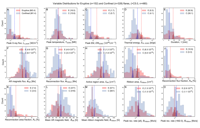
Figure 6: Appendix: Distributions of various physical variables for eruptive (red) and confined (blue) events ($>C5.0$ GOES flare class). Vertical dotted lines and numbers in the top right corner indicate mean value for each variable within eruptive and confined flare groups. Darker-color histograms show distributions of the mean, if we select $100$ random subsamples of the half of the events, and reflect variability of the mean due to event selection bias. See Appendix A for details.

In Figure 3(F-O) we analyze the distributions of magnetic properties. We find that confined flares have larger AR magnetic fluxes and areas (Figure 3F and Figure 3H). Confined flares have also larger mean magnetic field strengths within ribbon and AR areas (Figure 3L and Figure 3M). The above differences are consistent with magnetic cage interpretation, where ARs with large magnetic flux have confined eruptions. Practically, this means that for large flares of GOES class M1.0 and above: larger ARs, especially those with unsigned magnetic flux of $10^{23}$ Mx and above, tend to host confined flares; medium ARs with $3\times 10^{22}Mx<\Phi_{\mathrm{AR}}<10^{23}$ Mx host both confined and eruptive flares; smaller ARs with $\Phi_{\mathrm{AR}}<3\times 10^{22}$ Mx tend to host eruptive flares. Note that if we include smaller C-class flares, then we find that smaller active regions host a similar number of confined and eruptive flares (see Figure 6F in Appendix A).

From ribbon analysis, we find that the magnetic reconnection fluxes have similar distributions in both samples (Figure 3G), while the ribbon areas are larger for eruptive flares (Figure 3I). As a result, both reconnection flux and area fractions are larger for eruptive flares. These results are consistent with a scenario in which weaker strapping field makes flares more eruptive (Figure 3J and Figure 3K and also earlier works by e.g., Toriumi et al. 2017). Another factor that could explain why larger ARs host more confined flares is the relationship between AR size and access to periphery. Smaller regions have larger AR area fractions near their peripheries, with potentially better access to global field. In contrast, larger ARs have smaller AR area fractions near peripheries and hence tend to be more confined. Furthermore, the concept of closeness to periphery could explain why eruptive flares tend to have weaker magnetic fields, since the magnetic fields on AR peripheries are generally weaker. In contrast, confined flares are further from the periphery, where magnetic field is stronger, therefore mean magnetic field within ribbons for confined flares is stronger. The above results of larger magnetic field and smaller ribbon area within confined flares imply that in confined flares reconnection proceeds in more compact current sheets at lower coronal heights with larger field strengths. On the other hand, decreased magnetic field and increased ribbon area within eruptive flares implies that in eruptive flares reconnection proceeds in more extended current sheets at larger coronal heights with smaller magnetic field strengths.

Finally, we find that peak reconnection rates are slightly higher in confined vs. eruptive flares (Figures 3N and  3O). In other words, the same amount of reconnection flux, which we find to be very similar for eruptive and confined events in Figure 3G, gets reconnected at higher rates in confined events compared to eruptive flares (see Figure 3E). We hypothesize that the fact that confined flares are more compact and as a result occur lower in the corona involving stronger magnetic fields is the main factor that leads to increased peak reconnection rates in confined flares. At first, these results for the reconnection rates might seem different from Hinterreiter et al. (2018) and Tschernitz et al. (2018), who analyzed local peak reconnection flux rates (i.e. electric fields $E=v_{\mathrm{rbn}}B_{\mathrm{n}}$) and global peak reconnection flux rates in $50$ flares, finding that both are similar or higher in the eruptive flares compared to confined flares. We note, however, that our results here are for large flares above M1.0 with similar distributions of flare classes within confined and eruptive samples. In contrast, Hinterreiter et al. (2018) and Tschernitz et al. (2018) samples are very different, with flare class ranging from B to X-class flares and confined sample being much weaker than the eruptive one. Accounting for sample differences, we suggest that the two results would be consistent, i.e. a confined flare with similar reconnection and peak X-ray fluxes as an eruptive flare, would tend to have a higher peak reconnection rate than the eruptive flare. Figure 3(C) and Figure 7 in Tschernitz et al. (2018) confirm our guess, showing that for the same peak X-ray flux confined flares have higher peak reconnection rate.

3.2 Results: relationship between thermodynamic and magnetic properties in confined and eruptive flares

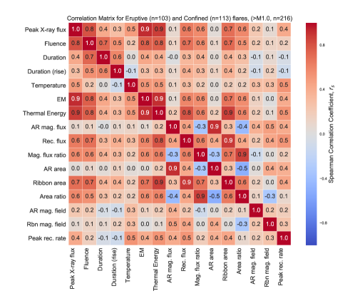
Figure 4: Results: Correlation matrix showing Spearman correlation coefficient, $r_{s}$, between different physical variables for all flares with GOES flare class $>M1.0$. We describe the qualitative strength of the correlation using the following guide: $r_{s}\in[0.2,0.39]$ – weak, $r_{s}\in[0.4,0.59]$ – moderate, $r_{s}\in[0.6,0.79]$ – strong, and $r_{s}\in[0.8,1.0]$ – very strong. See §3.2 for details.

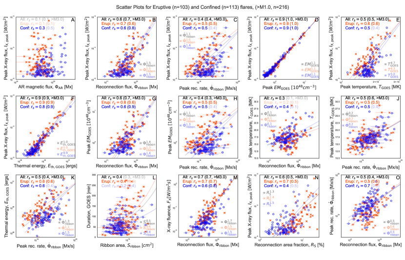
Figure 5: Results: Scatter plots between different physical variables for confined (blue) and eruptive (red) events ($>M1.0$ GOES flare class). In the corner we show Spearman correlation coefficient $r_{s}$ between each pair of plotted variables for all flares (black) and eruptive (red) and confined (blue) flares separately, where bold and dim fonts indicate statistical significance of the correlation with p-values below and above $p=0.01$, respectively. The values in the parentheses show values for flares above M3.0. See §3.2 for details.

In Figure 4 we show correlation matrix with Spearman correlation coefficients between all physical variables that we analyze in this paper. We show this matrix for illustrative purposes, to describe the relationship between all variables, especially those that we do not show in the scatter plots in Figure 5.

In Figure 5(A-F) we first analyze how peak X-ray flux scales with other variables and compare how confined and eruptive flare properties differ for a fixed peak X-ray flux.

The GOES peak X-ray flux has a moderate to high correlation with several thermodynamic properties, including peak temperature ($r_{s}=0.5$, Figure 5E), emission measure ($r_{s}=0.9$, Figure 5D) and thermal energy ($r_{s}=0.9$, Figure 5F). These correlations are in agreement with Feldman et al. (1996); Reep & Knizhnik (2019); Sadykov et al. (2019) and the standard chromospheric evaporation model (Hirayama, 1974), where GOES peak X-ray flux depends on the maximum EM.

The correlation between the AR magnetic flux and the peak X-ray flux is weak ($r_{s}=0.1$, Figure 5A) – larger active regions could host both large and small flares. In contrast the correlation between the peak X-ray flux and reconnection flux is strong ($r_{s}=0.6$ to $0.7$ for flares above M3.0, Figure 5B) in agreement with Kazachenko et al. (2017); Toriumi et al. (2017); Tschernitz et al. (2018), meaning that larger flares have larger amount of magnetic field participating in the reconnection. For flares above C1.0, Kazachenko et al. (2017) fit this relationship as $X_{\mathrm{peak}}\propto(\Phi_{\mathrm{ribbon}})^{1.5}$, while Reep & Knizhnik (2019) find similar $X_{\mathrm{peak}}\propto(\Phi_{\mathrm{ribbon]}})^{1.6}$. Here we find $X_{\mathrm{peak}}\propto(\Phi_{\mathrm{ribbon}})^{1.5}$ for both confined and eruptive flares, consistent with Kazachenko et al. 2017.

Since the reconnection flux is calculated cumulatively by adding the newly reconnected flux, as flare progresses, it is physically more appropriate to compare reconnection flux with cumulative GOES SXR flux, like SXR fluence. In the past, SXR fluence has been widely used to compare flare and CME energetics (e.g., Salas-Matamoros & Klein 2015). From Figure 5M we find that the correlation between the SXR fluence and reconnection flux is strong, $r_{s}=0.7$, only slightly above the correlation coefficient between GOES peak X-ray flux and reconnection flux ($r_{s}=0.6$). This result agrees with the previous study of Sindhuja et al. (2019) who found that reconnection flux has stronger correlations with fluence than with the peak X-ray flux: $r_{s}=0.8$ vs $r_{s}=0.6$ in their sample. In addition, we find that the flare peak X-ray flux has moderate correlation with flare area ratio and flux ratio ($r_{s}=0.6$, Figure 5N), in agreement with Kazachenko et al. 2017.

We find that the correlation between the peak X-ray flux and the peak reconnection flux rate is moderate, $r_{s}=0.4$ for both smaller and larger flares above M3.0 (Figure 5C), which is significantly weaker than correlation between peak X-ray flux and reconnection flux ($r_{s}=0.6$).

In Figures 5(G-H) we quantify how emission measure is related to other reconnection flux and its peak rate. As emission measure is very strongly correlated with the GOES peak X-ray flux ($r=0.9$), it has the same correlation coefficients with other variables as the GOES peak X-ray flux: strong correlations with reconnection flux ($r_{s}=0.6$, Figure 5G), ribbon area ($r_{s}=0.7$), flux ratio and area ratio ($r_{s}=0.6$) and moderate correlations with GOES temperature ($r_{s}=0.5$) and peak reconnection rate ($r_{s}=0.4$, Figure 5H).

For the first time, in Figures 5(I-J) we compare how GOES peak temperature is related to other reconnection properties. We find that the peak temperature has very weak correlation with the reconnection flux ($r_{s}=0.3$), which disappears for stronger flares ($r_{s}=0.1$ for flares above M3.0, Figure 5I). In contrast to reconnection fluxes, the peak temperature is sensitive to the peak reconnection rate with moderate to strong correlation coefficients, $r_{s}=0.5$ and $r_{s}=0.6$, for flares above $M1.0$ and $M3.0$, respectively (Figure 5J).

How does thermal energy scale with the reconnection flux? We find a strong to very strong correlation between the two ($r_{s}=0.8$), indicating that reconnection flux defines the thermal energy output of the flare. We find that the correlation between the thermal energy and the peak reconnection flux rate is weaker ($r_{s}=0.5$, Figure 5K), implying that the total reconnection flux has a stronger effect on the thermal energy than the peak reconnection rate, similar to the effect on the emission measure.

We find that flare duration has a moderate correlation with the flare ribbon area ($r_{s}=0.4$, Figure 5L). These results are consistent with statistical results by Toriumi et al. (2017); Reep & Knizhnik (2019) who found that in large flares above M5.0 flare durations scale with ribbon separation distances, while in weaker flares the correlation is weak (Reep & Knizhnik, 2019). One possible interpretation is that flare duration could be defined by the Alfvén transit time across the flaring area, which is related to ribbons’ size. In addition, the correlation between flare duration with flare ribbons size could be explained with the avalanche flare model (e.g., Lu & Hamilton 1991; Lu 1995): if a flare proceeds as a chain reaction of one reconnection event triggering others, then reconnecting larger flux would take more time.

Finally, in Figure 5O we look at the statistical relationship between the reconnection fluxes and peak reconnection flux rates. From this plot we find that the two variables are moderately correlated ($r_{s}=0.5$). We also find that for a fixed reconnection flux, confined flares have higher peak reconnection rates.

We then use scatter plots in Figure 5 to describe how variables within confined and eruptive samples differ for fixed flare class or emission measure. We find that for a fixed peak X-ray flux, confined flares have higher reconnection rates and peak temperatures (see Figures 5C and E). For thermal energies, only large confined flares, of flare class X1.0 and above, have higher thermal energies than eruptive flares (see Figure 5F).

These results are consistent with a qualitative scenario of energy partition between CME kinetic energy and flare thermal energy, where CME removes energy from the source region, leading to less thermal energy available for flares and lower peak flare temperatures in eruptive flares.

To improve our understanding of the underlying physical mechanisms driving the above correlations, we use a framework of extensive and intensive flare properties (Tan et al., 2007; Welsch et al., 2009; Bobra & Ilonidis, 2016; Kazachenko et al., 2022b).

Extensive properties are those that correlate or scale with flare size, described by peak X-ray flux or X-ray fluence, while intensive properties are those that do not scale with flare size. Above, we find the following extensive flare properties with a strong correlation with flare fluence, $F_{\mathrm{X}}$: peak X-ray flux, emission measure, thermal energy, reconnection flux and ribbon area: $r_{s}(F_{\mathrm{X}};[I_{\mathrm{peak}},EM_{\mathrm{GOES}},E_{\mathrm{th,GOES}},\Phi_{\mathrm{ribbon}},S_{\mathrm{ribbon}}])=[0.8,0.8,0.8,0.7,0.7]$. We also find that many extensive properties have a strong correlation with each other: e.g., $r_{s}(S_{\mathrm{ribbon}},[EM_{\mathrm{GOES}},E_{\mathrm{th,GOES}}])=[0.7,0.9]$.

Above, we also find some variables that behave more like intensive properties, such as temperature and reconnection flux rate. These properties do not exhibit a correlation with X-ray fluence, $r_{s}(F_{\mathrm{X}};[T_{\mathrm{GOES}},\dot{\Phi}_{\mathrm{ribbon}},])=[0.2,0.2]$, and only moderate correlations with peak X-ray flux: $r_{s}(I_{\mathrm{X,peak}};[T_{\mathrm{GOES}},\dot{\Phi}_{\mathrm{ribbon}},])=[0.5,0.4]$. However, both temperature and reconnection rate exhibit moderate correlation with each other: $r_{s}(T_{\mathrm{GOES}},\dot{\Phi}_{\mathrm{ribbon}})=0.5$.

What controls the plasma temperature and emission measure in flares? In Longcope et al. (2016, 2018), it is the reconnection rate that affects the maximum values of plasma properties. From our analysis we find that the temperature is more controlled by peak reconnection rate ($r_{s}=0.5$), while emission measure and thermal energy are more controlled by the reconnection flux ($r_{s}=0.6$ and $r_{s}=0.8$). For comparison the correlation between the reconnection flux and reconnection flux rate is only moderate ($r_{s}=0.5$, Figure 5O). These observational inferences are consistent with the framework of correlation between intensive and extensive flare properties above and case studies of temporally resolved profiles of reconnection rates, temperature and emissions (see e.g., Qiu et al. 2010; Qiu & Cheng 2022). For example, Qiu & Cheng (2022) analyzed $3$ eruptive and $3$ confined flares, finding that in all flares temperature rises and peaks early or co-temporal with the reconnection rate rise and peak.

In this section we focused on larger flares, of class $M1.0$, and above. Note that while variable distributions we find within confined and eruptive samples are not drastically different, the differences in the mean values are statistically persistent for different sub-samples (see darker-tone shaded histograms centered at dotted mean values in Figure 3). If we include flares $C5.0$ and above, as we do in Appendix A, we find similar physical conclusions in terms of flare magnetic and thermodynamic properties, with all the mean quantities being smaller due to smaller flare sizes. The main difference for flares within $C5.0-M1.0$ class vs. flares $M1.0$ and above, which we analyzed above, is that the fraction of confined flares drastically increases for flare class below $M1.0$, with fractions of confined flares of $80\%$ and higher as we go to lower flare class (see Appendix A for analysis including flares $>C5.0$). On the other hand, if we restrict our analysis to very large flares above $M5.0$, we find similar physical conclusions as for smaller flares; the only difference is in the duration distributions: confined flares have similar durations as eruptive flares for GOES classes $>M5.0$ (cf., for flares $>M1.0$ confined flares are slightly shorter).

4 Conclusions

We have compared magnetic and thermodynamics properties of 216 confined and eruptive flares of GOES class M1.0 and above (see Figures 3-5). In Appendix A we have also included smaller flares of GOES class C5.0 and above and analyzed properties in 480 flares.

What are the differences in average magnetic properties between large confined and eruptive flares? We find that:

• Eruptive flares have the same amount of reconnected flux as confined flares. However, unlike confined flares, they occur in smaller ARs with weaker magnetic field strengths. Their flare ribbons have weaker mean magnetic field strengths. As a result, they reconnect larger fractions of AR magnetic flux than confined flares.

• Confined flares occur in larger ARs with stronger mean magnetic field strengths compared to eruptive flares. Their ribbons are more compact, have stronger magnetic field strengths and reconnect smaller fractions of AR magnetic flux. Both of these results are consistent with earlier studies.

• For the first time, we find that for the same peak X-ray flux confined flares have higher mean peak reconnection rates than eruptive flares (see Figure 5C). This together with the fact that HXR (or microwave) emissions are temporally correlated with the global (see Qiu & Cheng 2022 and references therein) and local reconnection rates (Temmer et al., 2007; Naus et al., 2022), implies that large, eruptive flares are less efficient in particle acceleration than confined flares, in agreement with direct particle measurements (see e.g., Thalmann et al. 2015; Cai et al. 2021).

The above results support previously described main factors that define whether a flare would be confined or eruptive: (1) the strength of the overlying field, given by the AR flux, (2) the ratio between the reconnected magnetic flux and the active region flux and (3) the strength of the reconnected field (mean ribbon magnetic field). Here we have not investigated either ribbon field non-potentiality or its proximity to the AR edge, but previous works have shown that these differ in confined and eruptive flares (see summary in §1).

For flares of M-class and above, what are the differences in thermodynamic plasma properties between confined and eruptive flares? Our conclusions are as follows.

• Large eruptive flares have larger mean peak X-ray fluxes, peak emission measures and thermal energies. They have longer durations, and slightly smaller peak temperatures.

• Large confined flares have smaller mean peak X-ray fluxes, peak emission measures and thermal energies. They have shorter durations, and slightly larger peak temperatures.

• Why, for similar reconnection fluxes, do confined flares have larger temperatures and peak reconnection flux rates? We explain it with lower coronal altitudes and stronger reconnection fields in confined flares (since confined flares are more compact).

• Why, for similar reconnection fluxes, do confined flares tend to have shorter durations than eruptive flares? We explain it with the smaller physical size of confined flares (ribbon areas) and as a consequence shorter Alfvén transit time over the flaring area, than in eruptive flares (Reep & Knizhnik, 2019).

• We find that peak X-ray flux and emission measure are more strongly controlled by the reconnection fluxes than peak reconnection rates. On the other hand, peak temperature is more strongly controlled by the peak reconnection rate than the reconnection flux. This is consistent with temporally-resolved flare case studies that show temperature peaking early on together with the reconnection rate peak, while emission measure slowly rises to its maximum values as the cumulative reconnection flux increases (see e.g., Qiu & Cheng 2022).

To summarize, our findings indicate that, in general, in eruptive flares, reconnection proceeds more slowly in larger current sheets higher in the corona where the coronal magnetic field is weaker. In contrast, in confined flares, reconnection proceeds faster in more compact current sheets lower in the corona where the coronal magnetic field is stronger. As higher reconnection rates lead to more accelerated ions and electrons, large confined flares could be more efficient in producing ionizing electromagnetic radiation than eruptive flares. Given that flare high-energy radiation could affect exoplanet habitability conditions (Yamashiki et al., 2019; Airapetian et al., 2020), we speculate that confined flares could be important in shaping exoplanet conditions. This, together with a lack of CME detections on solar-like stars, would imply potentially a larger role of confined flares in exoplanet habitability.

In this section we focused on large flares of class $M1.0$ and above to have a similar number of eruptive and confined flares to analyze. Extending our analysis to flares of class $C5.0$ and above, we end up with a much larger fraction of confined flares, but find similar physical differences between magnetic/thermodynamic properties of confined/eruptive flares, with smaller mean values. For the results of our analysis for smaller flares, C5.0 and above, see Appendix A below.

The catalog is available online in IDL SAV and CSV file formats, and can be used for a wide spectrum of quantitative studies in the future, including case studies of the outliers.

We thank the reviewer for providing comments that have improved the manuscript. We thank the HMI team for providing us with the vector magnetic field SDO/HMI data. We thank the AIA team, in particular Marc DeRosa, for providing us with the UV SDO/AIA data. We thank the Croom Team for stimulating discussions. We thank the US taxpayers for providing the funding that made this research possible. We acknowledge support from NASA LWS NNH17ZDA001N, 80NSSC19K0070, NASA ECIP NNH18ZDA001N and NSF CAREER SPVKK1RC2MZ3.

Appendix A Expanding analysis from flares above M1.0 to flares above C5.0

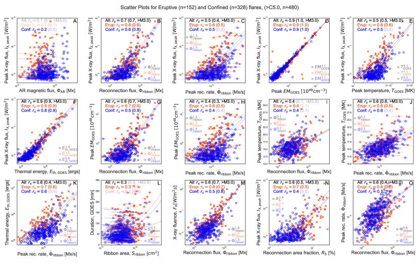
Figure 8: Appendix: Scatter plots: between different physical variables for confined (blue) and eruptive (red) events ($>C5.0$ GOES flare class). See Appendix A for details.

In addition to flares above M1.0, as has been analyzed in the main paper’s body, we extend our analysis to include smaller events with GOES class C5.0 and above. To minimize errors in the reconnection fluxes we restrict our analysis to events with reconnection flux imbalance between positive and negative polarities $\Phi_{\mathrm{ribbon,imb}}<20\%$. As a result we analyze 480 events, $152$ eruptive and $328$ confined flares, $C5.0$-class and above.

For flares of GOES class below M1.0, the fraction of confined flares significantly increases from $60\%$ for M1.0 flares to $85\%$ for C5.0 flares. As a result, the gap between distributions of GOES peak X-ray fluxes becomes even larger for confined and eruptive flares, affecting distributions of emission measure, thermal energy, etc. Nevertheless, except for mean reconnection fluxes that become smaller for confined than for eruptive flares, we observe the same tendencies between magnetic/thermodynamic properties for confined/eruptive flares as for flares above M1.0. Even the peak reconnection rates are smaller for eruptive than for confined flares, consistent with conclusions for larger flares.

References

- (1)
- Afanasyev et al. (2023) Afanasyev, A. N., Fan, Y., Kazachenko, M. D., & Cheung, M. C. M. 2023, ApJ, 952, 136
- Airapetian et al. (2020) Airapetian, V. S., Barnes, R., Cohen, O., et al. 2020, International Journal of Astrobiology, 19, 136
- Amari et al. (2018) Amari, T., Canou, A., Aly, J.-J., Delyon, F., & Alauzet, F. 2018, Nature, 554, 211
- Aschwanden et al. (2015) Aschwanden, M. J., Boerner, P., Ryan, D., et al. 2015, ApJ, 802, 53
- Aschwanden & Freeland (2012) Aschwanden, M. J., & Freeland, S. L. 2012, ApJ, 754, 112
- Aschwanden et al. (2017) Aschwanden, M. J., Caspi, A., Cohen, C. M. S., et al. 2017, The Astrophysical Journal, 836, 17
- Avallone & Sun (2020) Avallone, E. A., & Sun, X. 2020, ApJ, 893, 123
- Bateman (1978) Bateman, G. 1978, MHD instabilities
- Baumgartner et al. (2018) Baumgartner, C., Thalmann, J. K., & Veronig, A. M. 2018, ApJ, 853, 105
- Bobra & Ilonidis (2016) Bobra, M. G., & Ilonidis, S. 2016, ApJ, 821, 127
- Bornmann (1990) Bornmann, P. L. 1990, ApJ, 356, 733
- Brueckner et al. (1995) Brueckner, G. E., Howard, R. A., Koomen, M. J., et al. 1995, Sol. Phys., 162, 357
- Cai et al. (2021) Cai, Z. M., Zhang, Q. M., Ning, Z. J., Su, Y. N., & Ji, H. S. 2021, Sol. Phys., 296, 61
- Cheng et al. (2011) Cheng, X., Zhang, J., Ding, M. D., Guo, Y., & Su, J. T. 2011, ApJ, 732, 87
- Cui et al. (2018) Cui, Y., Wang, H., Xu, Y., & Liu, S. 2018, Journal of Geophysical Research (Space Physics), 123, 1704
- Derosa & Barnes (2018) Derosa, M. L., & Barnes, G. 2018, The Astrophysical Journal, 861, 131
- Emslie et al. (2005) Emslie, A. G., Dennis, B. R., Holman, G. D., & Hudson, H. S. 2005, Journal of Geophysical Research (Space Physics), 110, A11103
- Emslie et al. (2012) Emslie, A. G., Dennis, B. R., Shih, A. Y., et al. 2012, ApJ, 759, 71
- Feldman et al. (1996) Feldman, U., Doschek, G. A., Behring, W. E., & Phillips, K. J. H. 1996, ApJ, 460, 1034
- Gupta et al. (2021) Gupta, M., Thalmann, J. K., & Veronig, A. M. 2021, A&A, 653, A69
- Harra et al. (2016) Harra, L. K., Schrijver, C. J., Janvier, M., et al. 2016, Sol. Phys., 291, 1761
- Hassanin & Kliem (2016) Hassanin, A., & Kliem, B. 2016, ApJ, 832, 106
- Hassanin et al. (2022) Hassanin, A., Kliem, B., Seehafer, N., & Török, T. 2022, ApJ, 929, L23
- Hinterreiter et al. (2018) Hinterreiter, J., Veronig, A. M., Thalmann, J. K., Tschernitz, J., & Pötzi, W. 2018, Sol. Phys., 293, 38
- Hirayama (1974) Hirayama, T. 1974, Sol. Phys., 34, 323
- Hudson (2000) Hudson, H. S. 2000, ApJ, 531, L75
- Kahler & Ling (2022) Kahler, S. W., & Ling, A. G. 2022, ApJ, 934, 175
- Kay et al. (2003) Kay, H. R. M., Culhane, J. L., Harra, L. K., & Matthews, S. A. 2003, Advances in Space Research, 32, 1051
- Kazachenko et al. (2022a) Kazachenko, M. D., Albelo-Corchado, M. F., Tamburri, C. A., & Welsch, B. T. 2022a, Sol. Phys., 297, 59
- Kazachenko et al. (2012) Kazachenko, M. D., Canfield, R. C., Longcope, D. W., & Qiu, J. 2012, Sol. Phys., 277, 165
- Kazachenko et al. (2022b) Kazachenko, M. D., Lynch, B. J., Savcheva, A., Sun, X., & Welsch, B. T. 2022b, ApJ, 926, 56
- Kazachenko et al. (2017) Kazachenko, M. D., Lynch, B. J., Welsch, B. T., & Sun, X. 2017, ApJ, 845, 49
- Klein et al. (2010) Klein, K. L., Trottet, G., & Klassen, A. 2010, Sol. Phys., 263, 185
- Kliem et al. (2021) Kliem, B., Lee, J., Liu, R., et al. 2021, ApJ, 909, 91
- Kliem & Török (2006) Kliem, B., & Török, T. 2006, Physical Review Letters, 96, 255002
- Kurokawa (1989) Kurokawa, H. 1989, Space Sci. Rev., 51, 49
- Lemen et al. (2012) Lemen, J. R., Title, A. M., Akin, D. J., et al. 2012, Sol. Phys., 275, 17
- Li et al. (2021) Li, T., Chen, A., Hou, Y., et al. 2021, ApJ, 917, L29
- Li et al. (2020) Li, T., Hou, Y., Yang, S., et al. 2020, ApJ, 900, 128
- Li et al. (2022) Li, T., Sun, X., Hou, Y., et al. 2022, ApJ, 926, L14
- Liu et al. (2017) Liu, Y., Sun, X., Török, T., Titov, V. S., & Leake, J. E. 2017, The Astrophysical Journal, 846, L6
- Longcope et al. (2007) Longcope, D., Beveridge, C., Qiu, J., et al. 2007, Sol. Phys., 244, 45
- Longcope et al. (2016) Longcope, D., Qiu, J., & Brewer, J. 2016, ApJ, 833, 211
- Longcope et al. (2018) Longcope, D., Unverferth, J., Klein, C., McCarthy, M., & Priest, E. 2018, ApJ, 868, 148
- Lu (1995) Lu, E. T. 1995, ApJ, 446, L109
- Lu & Hamilton (1991) Lu, E. T., & Hamilton, R. J. 1991, ApJ, 380, L89
- Masson et al. (2017) Masson, S., Pariat, É., Valori, G., et al. 2017, A&A, 604, A76
- Moore et al. (2001) Moore, R. L., Sterling, A. C., Hudson, H. S., & Lemen, J. R. 2001, The Astrophysical Journal, 552, 833
- Moschou et al. (2019) Moschou, S.-P., Drake, J. J., Cohen, O., et al. 2019, ApJ, 877, 105
- Myers et al. (2015) Myers, C. E., Yamada, M., Ji, H., et al. 2015, Nature, 528, 526
- Namekata et al. (2022) Namekata, K., Ichimoto, K., Ishii, T. T., & Shibata, K. 2022, ApJ, 933, 209
- Naus et al. (2022) Naus, S. J., Qiu, J., DeVore, C. R., et al. 2022, ApJ, 926, 218
- Nita et al. (2004) Nita, G. M., Gary, D. E., & Lee, J. 2004, ApJ, 605, 528
- Plutino et al. (2023) Plutino, N., Berrilli, F., Del Moro, D., & Giovannelli, L. 2023, Advances in Space Research, 71, 2048
- Qiu & Cheng (2022) Qiu, J., & Cheng, J. 2022, Sol. Phys., 297, 80
- Qiu et al. (2010) Qiu, J., Liu, W., Hill, N., & Kazachenko, M. 2010, The Astrophysical Journal, 725, 319
- Reep & Knizhnik (2019) Reep, J. W., & Knizhnik, K. J. 2019, ApJ, 874, 157
- Reeves et al. (2010) Reeves, K. K., Linker, J. A., Mikić, Z., & Forbes, T. G. 2010, ApJ, 721, 1547
- Ryan et al. (2012) Ryan, D. F., Milligan, R. O., Gallagher, P. T., et al. 2012, ApJS, 202, 11
- Sadykov et al. (2019) Sadykov, V. M., Kosovichev, A. G., Kitiashvili, I. N., & Frolov, A. 2019, ApJ, 874, 19
- Salas-Matamoros & Klein (2015) Salas-Matamoros, C., & Klein, K.-L. 2015, Sol. Phys., 290, 1337
- Sindhuja & Gopalswamy (2020) Sindhuja, G., & Gopalswamy, N. 2020, The Astrophysical Journal, 889, 104
- Sindhuja et al. (2019) Sindhuja, G., Srivastava, N., Veronig, A. M., & Pötzi, W. 2019, MNRAS, 482, 3744
- Su et al. (2007) Su, Y., Golub, L., & Ballegooijen, A. A. V. 2007, The Astrophysical Journal, 655, 606
- Sun et al. (2022) Sun, X., Török, T., & DeRosa, M. L. 2022, MNRAS, 509, 5075
- Sun et al. (2015) Sun, X., Bobra, M. G., Hoeksema, J. T., et al. 2015, ApJ, 804, L28
- Tan et al. (2007) Tan, C., Jing, J., Abramenko, V. I., et al. 2007, ApJ, 665, 1460
- Tan et al. (2021) Tan, C.-M., Klein, K. L., Yan, Y.-H., et al. 2021, Research in Astronomy and Astrophysics, 21, 274
- Temmer (2021) Temmer, M. 2021, Living Reviews in Solar Physics, 18, 4
- Temmer et al. (2007) Temmer, M., Vršnak, B., & Veronig, A. M. 2007, Sol. Phys., 241, 371
- Thalmann et al. (2015) Thalmann, J. K., Su, Y., Temmer, M., & Veronig, A. M. 2015, ApJ, 801, L23
- Toriumi et al. (2017) Toriumi, S., Schrijver, C. J., Harra, L. K., Hudson, H., & Nagashima, K. 2017, The Astrophysical Journal, 834, 56
- Török & Kliem (2005) Török, T., & Kliem, B. 2005, ApJ, 630, L97
- Tschernitz et al. (2018) Tschernitz, J., Veronig, A. M., Thalmann, J. K., Hinterreiter, J., & Pötzi, W. 2018, ApJ, 853, 41
- Vasantharaju et al. (2018) Vasantharaju, N., Vemareddy, P., Ravindra, B., & Doddamani, V. H. 2018, ApJ, 860, 58
- Vemareddy (2019) Vemareddy, P. 2019, MNRAS, 486, 4936
- Veronig et al. (2021) Veronig, A. M., Odert, P., Leitzinger, M., et al. 2021, Nature Astronomy, 5, 697
- Veronig & Polanec (2015) Veronig, A. M., & Polanec, W. 2015, Solar Physics, 290.
- Wang et al. (2018) Wang, J., Simões, P. J. A., & Fletcher, L. 2018, ApJ, 859, 25
- Wang & Zhang (2007) Wang, Y., & Zhang, J. 2007, ApJ, 665, 1428
- Warmuth & Mann (2016) Warmuth, A., & Mann, G. 2016, A&A, 588, A115
- Webb & Hundhausen (1987) Webb, D. F., & Hundhausen, A. J. 1987, Sol. Phys., 108, 383
- Welsch et al. (2009) Welsch, B. T., Li, Y., Schuck, P. W., & Fisher, G. H. 2009, ApJ, 705, 821
- Yadav & Kazachenko (2023) Yadav, R., & Kazachenko, M. D. 2023, ApJ, 944, 215
- Yamashiki et al. (2019) Yamashiki, Y. A., Maehara, H., Airapetian, V., et al. 2019, ApJ, 881, 114
- Yashiro et al. (2006) Yashiro, S., Akiyama, S., Gopalswamy, N., & Howard, R. A. 2006, ApJ, 650, L143
- Yashiro et al. (2004) Yashiro, S., Gopalswamy, N., Michalek, G., et al. 2004, J. Geophys. Res., 109, A07105
- Zhu et al. (2020) Zhu, C., Qiu, J., Liewer, P., et al. 2020, The Astrophysical Journal, 893, 141
- Zuccarello et al. (2017) Zuccarello, F. P., Aulanier, G., Dudík, J., et al. 2017, ApJ, 837, 115