Stationarity without mean reversion: Improper Gaussian process regression and improper kernels

Abstract

Gaussian processes (GP) regression has gained substantial popularity in machine learning applications. The behavior of a GP regression depends on the choice of covariance function. Stationary covariance functions are favorite in machine learning applications. However, (non-periodic) stationary covariance functions are always mean reverting and can therefore exhibit pathological behavior when applied to data that does not relax to a fixed global mean value. In this paper, we show that it is possible to use improper GP prior with infinite variance to define processes that are stationary but not mean reverting. To this aim, we introduce a large class of improper kernels that can only be defined in this improper regime. Specifically, we introduce the Smooth Walk kernel, which produces infinitely smooth samples, and a family of improper Matérn kernels, which can be defined to be $j$-times differentiable for any integer $j$. The resulting posterior distributions can be computed analytically and it involves a simple correction of the usual formulas. By analyzing both synthetic and real data, we demonstrate that these improper kernels solve some known pathologies of mean reverting GP regression while retaining most of the favourable properties of ordinary smooth stationary kernels.

1 Introduction

Gaussian processes (GPs) are infinite-dimensional generalization of Gaussian distributions, which have gained widespread adoption in machine learning (Williams and Rasmussen, 2006), spatial statistics (Stein, 1999; Gelfand and Schliep, 2016) and statistical signal processing (Tobar et al., 2015; Lázaro-Gredilla et al., 2010; Ambrogioni and Maris, 2019, 2018; Tobar et al., 2023). In machine learning, GPs offer a mathematically tractable way to study neural networks at the limit of infinitely many hidden units (Neal and Neal, 1996), and provide robust non-parametric models for low-dimensional regression and classification problems (Williams and Rasmussen, 2006). In statistical signal processing, GPs are used to specify structured prior distributions on the underlying signals, which can be used to specify dynamic properties such as temporal smoothness and oscillatory frequency (Tobar et al., 2015). The properties of a GP depend on its covariance function, also known as kernel. Depending on its covariance function, samples from a GP can exhibit a wide range of behaviors such as polynomial growth, quasi-periodic oscillations, fractality or smoothness.

In machine learning, most commonly used covariance functions are stationary and isotropic. As we shall see in the paper, stationary covariance functions usually induce mean-reversion, meaning that perturbations tend to ’relax’ towards a fixed average value. Indeed, several real-world phenomena are mean-reverting. For example, fluctuations in blood pressure show mean-reversion in healthy humans due to homeostatic regulation. On the other hand, other real-world timeseries such as stock prices do not show mean reversion, since today’s price is the best prediction for future prices. Since many real-world processes are not mean-reverting, it is often useful to choose covariance functions that do not induce this property. Unfortunately, stationary covariance functions either are mean-reverting or induce oscillations around a determined central point. Therefore, when mean-reversion is not desirable, the user is forced to use non-stationary kernels, which usually involve some rigid and rather arbitrary assumptions. For example, polynomial covariance functions force the samples to be a $d$-degree polynomials, while Brownian motion covariance functions are much more flexible but require the pre-specification of a starting point for the random-walk process.

In this paper, we show that it is possible to use kernels that are both stationary and not mean-reverting as far as we use improper GP priors. Roughly speaking, an improper GP has infinite variance everywhere and its distribution of values at any point is given by an (improper) flat distribution. However, like for improper priors in univariate Gaussian inference, the resulting posterior distribution is a proper GP when conditioned on at least one data-point. By taking the limit of an infinite constant shift on the covariance function, we derive closed-form matrix formulas for the posterior mean and covariance matrix of a GP regression with improper GP prior. We also show that, at this limit, new improper kernels can be used to construct the covariance functions. These improper kernels do not correspond to valid covariance functions for any finite constant shift, but they are valid at the limit of an infinite shift. Importantly, we show that these improper kernels can induce processes that are both stationary and not mean-reverting. We introduce a large class of improper kernels that generalizes the Matérn class to this improper regime.

2 Preliminaries

In this section, we will review some preliminary concepts related to GP regression, covariance functions and the use of improper prior distributions.

2.1 Improper Gaussian priors

The use of improper priors is well-established in Bayesian statistics and machine learning. Loosely speaking, an improper prior is a non-normalizable density that nevertheless provides a proper normalizable posterior. Improper priors are often used as uninformative prior models.

For example, consider a univariate Gaussian inference with prior $\mathcal{N}(x;0,\nu^{2})$ and likelihood $\mathcal{N}(y;x,\sigma^{2})$. Given a data-point $y$, the resulting posterior distribution over $x$ is

$$p_{\nu}(x\mid y)=\mathcal{N}\!\left(x;\frac{\sigma^{-2}}{\nu^{-2}+\sigma^{-2}}y,(\nu^{-2}+\sigma^{-2})^{-1}\right)~{}.$$ (1)

In this case, the posterior provides a biased estimator of the mean since the data $y$ is ”shrank” towards the origin (i.e. the prior mean). In order to remove the bias, we can take the limit $\nu^{2}\rightarrow\infty$, which corresponds to an uninformative improper prior with infinite variance. However, while the prior does not exist as a proper probability distribution, the posterior has a well-defined (normalized) limit

$$p_{\infty}(x\mid y)=\mathcal{N}\!\left(x;y,\sigma^{2}\right)~{},$$ (2)

which provides an unbiased estimator of the mean.

2.2 Gaussian process regression

Consider a dataset comprised of $N$ pairs $\{(\boldsymbol{x}_{1},y_{1}),\dots,(\boldsymbol{x}_{k},y_{k}),\dots(\boldsymbol{x}_{N},y_{N})\}$, where $\boldsymbol{x}_{k}$ is a $D$-dimensional vector of predictors and $y_{k}$ is a scalar dependent variable. In a non-parametric regression problem, we assume the output variable $y_{k}$ to be sampled from an underlying unknown function $f:\mathds{R}^{D}\rightarrow\mathds{R}$ and corrupted with Gaussian white noise $\epsilon_{k}$ with variance $\sigma^{2}$:

$$y_{k}=f(\boldsymbol{x}_{k})+\epsilon_{k}~{}.$$ (3)

The resulting non-parametric regression problem can be solved in closed-form is we assign a GP prior to the functional space:

$$f(\boldsymbol{x})\sim\mathcal{GP}\left(m(\boldsymbol{x}),k(\boldsymbol{x}^{\prime},\boldsymbol{x}^{\prime\prime})\right)~{},$$ (4)

where the prior process is defined by the mean function $m(\boldsymbol{x})$ and by the covariance function $k(\boldsymbol{x}^{\prime},\boldsymbol{x}^{\prime\prime})$. For the prior to be well-posed, the covariance function needs to be positive definite, meaning that all possible $M$-dimensional matrices obtained from it by evaluating it on a list of predictors are symmetric and positive-definite. in fact, if we restrict our attention on the set of predictors $\{\boldsymbol{x}_{1},\dots,\boldsymbol{x}_{N}\}$, this functional prior reduces to a conventional multivariate Gaussian:

$$\boldsymbol{f}\sim\mathcal{N}\left(\boldsymbol{m},K\right)~{},$$ (5)

with $f_{k}=f(\boldsymbol{x}_{k})$, $m_{k}=m(\boldsymbol{x}_{k})$ and $K_{jk}=k(\boldsymbol{x}_{j},\boldsymbol{x}_{k})$. In the following, we will assume the mean function to be identically equal to zero. However, all results can be easily adapted to the case of non-zero mean function. Given the dataset and an arbitrary set of $K$ queries $\{\boldsymbol{x}_{1}^{*},\dots,\boldsymbol{x}_{K}^{*}\}$, we can write down the posterior probability of the values of the function at the query points:

$$\boldsymbol{f}^{*} \mid\{(\boldsymbol{x}_{1},y_{1}),\dots,(\boldsymbol{x}_{N},y_{N})\}$$ (6)

$$\sim\mathcal{N}\left(\boldsymbol{m}_{\text{post}},K_{\text{post}}\right)~{},$$

with

$$\boldsymbol{m}_{\text{post}}=K^{*}(K+\sigma^{2}I)^{-1}\boldsymbol{y}$$ (7)

and

$$K_{\text{post}}=K^{**}-K^{*}(K+\sigma^{2}I)^{-1}{K^{*}}^{T}~{}.$$ (8)

In these expressions, the matrix $K^{**}_{jk}=k(\boldsymbol{x}^{*}_{j},\boldsymbol{x}^{*}_{k})$ is the (auto-)covariance matrix for the query set and the matrix $K^{*}_{jk}=k(\boldsymbol{x}^{*}_{j},\boldsymbol{x}_{k})$ is the cross-covariance matrix between the training set and the query set.

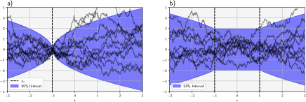
Figure 1: Samples and $95\%$ probability intervals of a) bilateral Brownian motion starting at $-1$ and b) superposition of two bilateral Brownian motions starting at $-1$ and $1$ respectively. Note the ’stationary’ interval with constant variance in between the two points.

3 Stationarity and mean-reversion

In the following sections, we will restrict our attention to $1$-dimensional signals and we will denote the dependent variable as $t$. We will generalize most of the results to higher dimensional spaces in Sec. 9.

A covariance function $k:\mathds{R}\times\mathds{R}\rightarrow\mathds{R}$ is said to be stationary if it solely depends on the difference between the two input values:

$$k(t,t^{\prime})=\hat{k}(\tau)$$ (9)

where $\tau=t^{\prime}-t$ and $\hat{k}:\mathds{R}\rightarrow\mathds{R}$. Stationary covariance functions are extremely common in the machine learning literature since they do not require ad hoc assumptions regarding the location-dependent statistical properties of the data. A well-known example of stationary covariance function is the (misleadingly named) Squared Exponential:

$$\hat{k}_{\text{se}}(\tau)=e^{-\frac{\tau^{2}}{2l^{2}}}$$ (10)

where $l$ is a length-scale parameter that regulates how fast the correlation between two points declines as a function of their distance. We say that a stationary covariance function is regular if $\hat{k}(\tau)$ is absolutely integrable, meaning that $\int_{0}^{\infty}|\hat{k}(\tau)|\text{d}\rho<\infty$. From this, we can deduce that, if the covariance function is regular, $\lim_{\rho\rightarrow\infty}\hat{k}(\tau)=0$, since otherwise the integral would not converge. Stationary covariance functions are fully determined by their associated spectral density:

$$\tilde{k}(\omega)=\int_{-\infty}^{+\infty}\hat{k}(\tau)e^{-i\omega\tau}\text{d}\tau~{},$$ (11)

which is a real-valued function since the kernel is symmetric. The constraint of positive-definiteness implies that the spectral density is positive-valued.

A covariance function is said to be mean-reverting if, for any $t$, the resulting stochastic process respects the following property

$$\lim_{\tau\rightarrow\infty}\mathbb{E}\!\left[f(t)\mid f(t-\tau)\right]=\mathbb{E}\!\left[f(t)\right]~{},$$ (12)

In other words, in a mean-reverting process the conditional mean function always converges to the unconditional mean for points far away from the conditioning set. From the point of view of machine learning, this imply that the information provided by each data-point is local, since distant data points have negligible impact on the posterior distribution of a query point. While this assumption may seem reasonable, it does violate a basic principle of prediction: in the absence of further information, the most likely value of a variable in the future is its value in the present. For example, if our goal is to predict the performance of a student during college given the fact that she has very high grades in primary school, it is safer to assume that the performance will on average stay high instead of assuming that it will revert back to the population average. The assumption of mean reversion is also violated by many well-known and high-performance machine learning techniques. For example, in $k$-nearest neighbors regression and classification, the nearest training point is used to make a non-trivial prediction regardless to its distance from the query point (Taunk et al., 2019). Similarly, methods such as binary trees, random forests and adaptive boosting exhibit a similar non-mean-reverting behavior (Sutton, 2005; Fawagreh et al., 2014). Finally, parametric regression models such as linear models, polynomial regression models and neural networks all tend to extrapolate their prediction away from the training data in a non-mean-reverting manner (Maulud and Abdulazeez, 2020).

Given this, it is perhaps surprising that almost all applications of GP regression and classification to machine learning use mean-reverting covariance functions such as the Squared Exponential and the Matérn class . As we discussed above, the most likely reason for this choice is that stationary covariance functions tend to be less arbitrary and less dependent on domain knowledge. However, it is easy to show that all regular stationary covariance functions are mean-reverting. Let us assume for simplicity that the mean function is identically equal to zero. In this case, the posterior mean function of a stationary GP regression (or classification) can always be written as follows

$$\mu_{\text{post}}(t)=\sum_{j=1}^{m}w_{j}\hat{k}(t-t_{n})~{},$$ (13)

where the $\boldsymbol{x}_{n}$ is a training point and $w_{n}$ is a real-valued weight. Since the covariance function is regular, we know that $\lim_{\tau\rightarrow\infty}\hat{k}(\tau)=0$. This implies that $\mu_{\text{post}}(t)$ converges to the mean function (which we assumed to be identically equal to zero) as the distance between $t$ and the closest training point increases. This reasoning can be easily generalized to the case with a non-zero mean function. Note that this property does not necessarily hold for non-regular stationary covariance functions. In the machine learning literature, the most common examples of non-regular stationary covariance functions are the cosine and the periodic, which are both periodic with a spectral density defined as a mixture of delta distributions. In this case, the posterior expectation is itself periodic and it does not converge to any fixed value for $\rho\rightarrow\infty$, but instead it oscillates around the prior mean (or around a biased estimate of the data mean in the case of the periodic covariance functions).

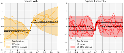
Figure 2: Posterior expectation and $95\%$ intervals and samples of a GP conditioned on two data-points with A) improper Smooth Walk prior (top figure) and B) proper Squared Exponential prior. The length scale was $0.2$ for both models. The black line show the ground-truth signal $\text{sign}(t)$.

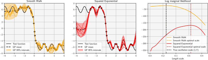
Figure 3: Posterior expectation and $95\%$ interval of a GP regression with ground-truth signal $\sin(6t)+0.4t-5\tanh(t)$ with noise level $\sigma=0.05$. The length scale was selected by optimizing the marginal likelihood conditioned on one data point (see rightmost panel).

4 An intuitive introduction to stationary improper Gaussian processes

Consider a (bilateral) Brownian motion process $z(t)$, which crosses the $y$-axis at $t_{0}$. This process is characterized by the following covariance function:

$$k_{t_{0}}(t,t^{\prime})=\frac{1}{2}\left(|t-t_{0}|+|t^{\prime}-t_{0}|-|t^{\prime}-t|\right)~{}.$$ (14)

This process is not stationary since the covariance cannot be expressed as a function of the time difference $t^{\prime}-t$. The lack of stationarity comes from the fact that the process is forced to cross the $y$-axis at $t_{0}$, which implies that the variance of the process is not translationally invariant. In fact, the variance of the process increases without bounds for $|t|\rightarrow\infty$ (see Fig. . 1 a ).

In order to make a stationary process, we can consider the average of two bilateral Brownian processes with starting points equal to $\tau$ and $-\tau$ respectively, where $\tau$ is a free parameter. This leads to a new process characterized by the following covariance function:

$$k_{\tau}(t,t^{\prime})=\frac{1}{2}\left(k_{\tau}(t,t^{\prime})+k_{-\tau}(t,t^{\prime})\right)~{}.$$ (15)

As shown in Fig. 1 b, the standard deviation of this process is constantly equal to $\tau$ and increases for $t>\tau$ and $t<-\tau$. In particular, for $t,t^{\prime}\in(-\tau,\tau)$, the covariance is given by $\tau-|t^{\prime}-t|$. Therefore, the process is indeed stationary within this interval. We can now obtain a globally stationary process by taking the limit $\tau\rightarrow\infty$, using a suggestive but improper notation, we can write the resulting covariance function as

$$k_{\infty}(t,t^{\prime})=\infty-|t^{\prime}-t|~{},$$ (16)

where the infinity symbol reminds us that the variance of the process is infinite everywhere. Intuitively, this covariance describes a Brownian motion without a starting point. In the following section, we will formalize this intuitive reasoning in the context of improper GP regression.

5 Improper Gaussian process regression

In this section, we will derive the formula for the posterior of an improper Gaussian process regression, where the variance of the prior process is infinite everywhere. We start by writing the covariance function of the process as follows:

$$k(t,t^{\prime})=s(t,t^{\prime})+c$$ (17)

where $c$ an arbitrary constant that we will tend to infinity in the derivation. We denote the function $s(t,t^{\prime})$ as the improper kernel of the process. In order to give rise to a well-posed improper GP prior, the function $s(t,t^{\prime})$ needs to satisfy the following definition:

Definition 5.1 (improper kernel).

A $s(t,t^{\prime}):\mathbb{R}\times\mathbb{R}\rightarrow\mathbb{R}$ is a improper kernel when, for all $m\times m$ finite sub-matrices with $S_{ij}=s(t_{i},t_{j})$, we have that $S$ is symmetric and $\mathbf{u}^{T}S\mathbf{u}\geq 0$ when $\mathbf{u}\perp\mathbf{1}_{m}$, where $\mathbf{1}_{m}=(1,\dots,1)\in\mathbb{R}^{m}$ is the constant one vector in the appropriate space.

In the definition, $\boldsymbol{u}\perp\boldsymbol{1}_{m}$ means that $\sum_{j=1}^{m}u_{j}=0$. Note that this property is less restrictive than the standard positive (semi-)definiteness property.

From Def. 5.1, we can show that every $m$-dimensional covariance matrix obtained from Eq. 17 is positive definite as far as the constant $c$ is large enough. In fact, the covariance matrix can be decomposed as follows

$$K=S+c\mathbf{1}_{m}\mathbf{1}_{m}^{T}$$ (18)

where $\mathbf{1}_{m}$ is again a vector with constant elements all equal to $1$. Using the definition, we obtain

$$\mathbf{u}^{T}K\mathbf{u}=\mathbf{u}^{T}S\mathbf{u}+m^{2}c~{},$$

which can be made positive for large enough values of $c$, since $\mathbf{u}^{T}S\mathbf{u}$ is finite.

Let us now assume to have a $m$-dimensional vector $\mathbf{y}$ of observations of the dependent variable corresponding to the $m$ input points $\{t_{1},\dots,t_{m}\}$. Assuming uncorrelated observation noise with variance $\sigma^{2}$ and that the value of $c$ has been chosen to make the covariance matrix positive-definite, the posterior expectation of the corresponding GP regression evaluated at the $n$ query points $\{t^{*}_{1},\dots t^{*}_{n}\}$ is given by the formula

$$\mu_{\text{post}}=(S^{*}+c\mathbf{1}_{n}\mathbf{1}_{m}^{T})(\Sigma+c\mathbf{1}_{m}\mathbf{1}_{m}^{T})^{-1}\textbf{y}~{},$$ (19)

where $S^{*}_{ij}=s(t^{*}_{i},t_{j})$ and $\Sigma=S+\sigma^{2}I$. We can now obtain the expectation formula for the improper regression by taking the limit $c\rightarrow\infty$. Assuming $\Sigma$ to be invertible, this can be done by first applying the Sherman–Morrison formula to the matrix inverse:

$$(\Sigma+c\mathbf{1}_{m}\mathbf{1}_{m}^{T})^{-1}=\Sigma^{-1}-c\frac{\Sigma^{-1}\mathbf{1}_{m}\mathbf{1}_{m}^{T}\Sigma^{-1}}{1+c\mathbf{1}_{m}^{T}\Sigma^{-1}\mathbf{1}_{m}}~{}.$$ (20)

We can now plus Eq. 20 in Eq. 19 and take the limit, leading to the formula:

$$\mu_{\text{post}}=S^{*}\Sigma^{-1}\mathbf{y}-S^{*}\frac{\Sigma^{-1}\mathbf{1}_{m}\mathbf{1}_{m}^{T}\Sigma^{-1}}{\mathbf{1}_{m}^{T}\Sigma^{-1}\mathbf{1}_{m}}\mathbf{y}+\frac{\mathbf{1}_{m}\mathbf{1}_{m}^{T}\Sigma^{-1}}{\mathbf{1}_{m}^{T}\Sigma^{-1}\mathbf{1}_{m}}\mathbf{y}$$ (21)

where the first term is identical to the posterior expectation formula of a regular GP regression except for the fact that $\Sigma$ is not necessarily positive-definite. Similarly, by taking the limit we can obtain a finite expression for the posterior covariance. To simplify the expression of the formula, we denote the matrix obtained by evaluating the improper kernel at the query points as $S^{**}_{ij}=s(t_{j}^{*},t_{k}^{*})$ and define the uncorrected covariance matrix as $\tilde{K}_{\text{post}}=S^{**}-S^{*}\Sigma^{-1}{S^{*}}^{T}$. We can now write the correct posterior covariance as the uncorrected covariance plus a correction term:

$$K_{\text{post}}=\tilde{K}_{\text{post}}+FF^{T}/(\boldsymbol{1}_{m}^{T}\Sigma^{-1}\boldsymbol{1}_{m})$$ (22)

where $F=\boldsymbol{1}_{n}-K^{*}\Sigma^{-1}\boldsymbol{1}_{m}$.

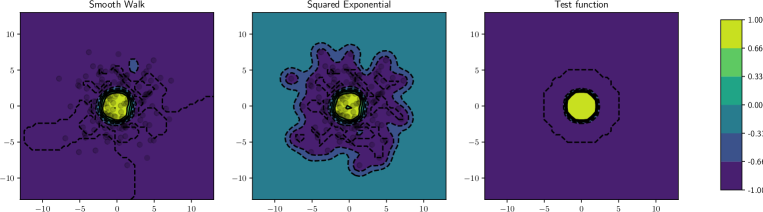
Figure 4: Posterior expectation of a two-dimensional GP regression with ground-truth signal (test function) $\tanh(-x^{2}-y^{2}+5)$. The posterior expectation with the Squared Exponential prior reverses to the prior mean while the bivariate Smooth Walk expectation stays close to the nearest data-point.

6 Stationary improper kernels

Since any positive kernel automatically fulfils the improper kernel property, the formulas given in the previous section can be used together with ordinary covariance functions. In that case, like in the case of an ordinary improper Gaussian prior, the mean posterior expectation provides an unbiased (unregularized) estimate of the mean of the true signal. However, the biggest potential advantage of the approach comes from new improper kernels that are not positive definite and have properties that cannot be obtained with positive-definite kernels. In Section 4, we saw that, up to an infinite additive constant, the negative absolute difference $-|t^{\prime}-t|$ can be seen as the (improper) kernel of a stationary Browning motion without starting points:

$$s_{\text{bm}}(t,t^{\prime})=\hat{s}_{\text{bm}}(\tau)=-|\tau|$$ (23)

In words, the improper stationary kernel is simply the (negative) distance between the points. In Supp. D, we prove that 23 respect definition 5.1. The proof rely on the theory of tempered distributions, which is used to obtained the spectral density

$$\tilde{s}_{\text{bm}}(\omega)=\sqrt{\frac{2}{\pi}}\cdot\frac{1}{\omega^{2}}~{},$$ (24)

which can be interpreted as the distributional Fourier transform of the negative absolute value function (Strichartz, 2003). However, it is important to keep in mind that $1/\omega^{2}$ is not a true density since it is not defined, and more importantly not integrable, at $\omega=0$. This issue can be circumvented using a technique called Hadamard regularization (see Supp. B), which can be used to assign a value to the divergent integral. However,this can lead to some rather counterintuitive behavior, for example, if we integrate Eq. 24 against a positive-valued test function on an interval including $\omega=0$, we can obtain a negative result! This strange behavior is the reason why the kernel is not positive-definite, and plays a central role in the proof. Samples from this kernel inherit the familiar properties of Brownian motions. As an example, since $\hat{s}(\rho)$ is continuous but not differentiable at the origin, the process is mean-squared continuous but not mean-squared differentiable. Importantly, like ordinary Brownian motions, the process is not mean-reverting.

7 The Smooth Walk kernel

In many applications, it is beneficial to use smooth covariance functions capable of extrapolating linear and higher order trends in the data. In this section, we will therefore introduce an infinitely smooth improper kernel that does not induce mean reversion. The idea is then to find a relaxation of the absolute value that is infinitely differentiable at the origin. The identity $|x|=x\text{sign}{x}$ suggests that we can do this by replacing the sign function with a hyperbolic tangent. This leads to the following kernel:

$$s_{\text{sw}}(t,t^{\prime};l)=-(t^{\prime}-t)\tanh{\left((t^{\prime}-t)/l\right)}$$ (25)

where $l$ is a length scale parameter. We named it Smooth Walk (improper) kernel since, as we shall see, it behaves like a smooth random walk. In Supp. D, we prove that this is indeed a improper kernel for all positive values of $l$. The proof is analogous to the one discussed in the previous section and it relies on the fact that the distributional Fourier transform of $x\tanh{x}$ can be expressed using the density:

$$\tilde{s}_{\text{sw}}(\omega;l)=\frac{\pi^{3/2}}{2\sqrt{2}}\frac{l^{2}\coth(l~{}\omega\pi/2)}{\sinh(l~{}\omega\pi/2)}~{},$$ (26)

which, like $1/\omega^{2}$, is not defined and not locally integrable at $\omega=0$. In fact, we have that $\tilde{s}_{\text{sw}}(\omega;l)\sim\omega^{-2}/(2\sqrt{2})$ for $\lim\omega\rightarrow 0$. From this, it follows that $s_{\text{sw}}(\boldsymbol{x},\boldsymbol{x}^{\prime};l)$ is not a positive-definite kernel, since the singularity in the density results in a (usually large) negative eigenvalue in the Gram matrices. Since $x\tanh{x}$ is infinitely differentiable at $t=0$, the resulting process is infinitely mean-squared differentiable and exhibits very smooth samples. In this sense, the Smooth Walk improper kernel is similar the the Squared Exponential covariance function. However, like the Brownian motion kernel, the Smooth Walk kernel does not exhibit mean reversion, as can be seen in Fig. 2, which show the posterior expectation and intervals of a Smooth Walk and a Square Exponential process (with identical length scale) given two datapoints.

	SW (i)	MW 1/2 (i)	GW (i)	SE (p)	M 1/2 (p)	M 3/2 (p)
Mean NNL	10.34	5.89	3.90	76.02	74.23	74.78
SEM	2.09	0.79	0.07	21.35	21.58	21.19

Table 1: Quantitative results of the stock prices forecasting experiment. SW (i): Smooth Walk (improper), MW 1/2 (i): Matérn Walk 1/2, GW (i): Gaussian Walk, SE (p): Squared Exponential (proper), M 1/2: Matérn 1/2 (proper), M 3/2: Matérn 3/2 (proper).

8 Convolution kernels and the improper Matérn class

In this section, we will introduce a general technique to construct improper kernels that replicate the behavior of existing stationary covariance functions. The main idea is to smooth out $-|t|$ by convolving it with a another (proper) kernel $\tilde{k}(\tau)$:

$$\hat{s}_{\hat{k}}(\tau)=-\int_{-\infty}^{+\infty}|w|\hat{k}(\tau-w)\text{d}w$$ (27)

Due to the convolution theorem, we know that the spectral density associated to this convoluted kernel is

$$\tilde{s}_{\hat{k}}(\omega)=\sqrt{\frac{2}{\pi}}\frac{\hat{k}(\omega)}{\omega^{2}}~{},$$ (28)

which is again singular at $0$ (at least if $\hat{k}(\omega)=0$) and well-defined and non-negative valued everywhere else. This implies that Eq. 28 gives us a valid (improper) kernel.

We can now use this formula to construct improper kernels with different levels of smoothness. In general, if $\hat{k}(\tau)$ is $j-1$-times differentiable at $0$, we have that $\hat{s}_{\hat{k}}(\tau)$ is $p$-times differentiable at the origin. This implies that the resulting process is $j$-times mean-squared differentiable.

We can now introduce the following Matérn Walk family of improper kernels:

$$\hat{s}_{j}(\tau)=-\int_{-\infty}^{+\infty}|w|\hat{\mathcal{M}}_{j-1/2}((\tau-w)/l)\text{d}w$$ (29)

where $l$ is a length scale hyper-parameter and $\hat{\mathcal{M}}_{\nu}(\tau)$ is the Matérn class kernel, which is defined in terms of modified Bessel functions (Stein, 1999). While the general expression involves special functions, this kernel greatly simplifies for $\nu=p+1/2$ with $p$ being an integer. In this case, the kernel can be expressed as a product of an exponential and a polynomial of order $p$. Importantly, for this class of functions we can compute the convolution in closed-form. For example $\hat{m}_{1/2}(\tau/s)=e^{-|\tau|/s}$, which leads to the improper kernel:

$$\hat{s}_{1}(\tau)=-2\left(|\tau|+l~{}e^{-|\tau|/s}\right)~{},$$ (30)

which as expected is once differentiable at the origin. Another interesting special case is given by the limit $j\rightarrow\infty$. In this case, the Matérn converges to a Squared Exponential and the resulting improper kernel is

$$\hat{s}_{\infty}(\tau)=-\sqrt{\frac{2}{\pi}}e^{-\frac{\tau^{2}}{2l^{2}}}-(\tau/l)~{}\text{erf}(\tau/(\sqrt{2}l))~{},$$ (31)

which is an improper version of the infinitely differentiable Squared Exponential kernel. As will refer to this kernel as Gaussian Walk (GW) and to other members of the class as Matérn Walk (MW).

	road	auto	bike	concrete	energy	forest
SE (p)	1	1	1	1	1	1
M 1/2 (p)	0.90	0.87	1.04	4.23	1.60	1
M 3/2 (p)	0.95	0.91	1.01	2.16	0.88	1
SW (i)	0.91	0.98	0.93	0.36	0.83	0.97
MW 1/2 (i)	0.90	0.99	0.94	0.23	0.79	0.97
GW (i)	0.98	0.98	0.96	0.26	0.87	0.97

Table 2: Results of five multivariate regression problems from the UCI bachmark. Test set performance is reported as the ratio between the MSE of the model and the MSE obtained with a proper SE kernel. SW (i): Smooth Walk (improper), MW 1/2 (i): Matérn Walk 1/2, GW (i): Gaussian Walk, SE (p): Squared Exponential (proper), M 1/2: Matérn 1/2 (proper), M 3/2: Matérn 3/2 (proper).

9 Improper isotropic kernels in high-dimensional spaces

In this section, we will denote a $d$-dimensional vector as $\boldsymbol{x}\in\mathds{R}^{d}$. The improper kernels introduced in this paper can be generalized to higher dimensional spaces. A natural choice is to use an isotropic kernels. A kernel $k:\mathds{R}^{D}\times\mathds{R}^{D}\rightarrow\mathds{R}$ is said to be isotropic if the covariance of the process at two points can be expressed as a function of the Euclidean distance that separates them:

$$k(\boldsymbol{x}^{\prime},\boldsymbol{x})=k_{\text{iso}}({\left\lVert\boldsymbol{x}^{\prime}-\boldsymbol{x}\right\rVert}_{2})~{},$$ (32)

where $\hat{k}_{\text{iso}}\mathds{R}\rightarrow\mathds{R}$. It is straightforward to ’lift’ a $1$-dimensional stationary kernel to a $d$-dimensional isotropic kernel. For example, we can define the isotropic version of the Brownian motion improper kernel as follows:

$$s_{\text{bm}}^{(d)}(\boldsymbol{x},\boldsymbol{x}^{\prime})=\hat{s}_{\text{bm}}({\left\lVert\boldsymbol{x}^{\prime}-\boldsymbol{x}\right\rVert}_{2})~{}.$$ (33)

Unfortunately, the resulting spectral density depends on the dimensionality and cannot easily be obtained from the univariate spectral density. As proven in (Stein and Weiss, 1971), the spectral density of $s_{\text{bm}}^{(d)}$ is given by the following distribution:

$$\tilde{s}_{\text{bm}}^{(d)}(\boldsymbol{\omega})=2^{d+1}\frac{\Gamma((d+1)/2)}{\Gamma(-1/2)}{{\left\lVert\omega\right\rVert}_{2}^{-(d+1)}}~{},$$ (34)

which is again positive-valued up to a singularity at $\boldsymbol{\omega}$ that needs to be regularized. The Smooth Walk kernel can also be generalized into an isotropic kernel:

$$s_{\text{sw}}^{(d)}(\boldsymbol{x},\boldsymbol{x}^{\prime};l)=-{\left\lVert\boldsymbol{x}^{\prime}-\boldsymbol{x}\right\rVert}_{2}\tanh{\left({\left\lVert\boldsymbol{x}^{\prime}-\boldsymbol{x}\right\rVert}_{2}/l\right)}~{},$$ (35)

Unfortunately, we were not able to obtain the spectral density analytically and we therefore cannot rigorously prove that this is indeed a valid improper kernel. However, we ran a comprehensive numerical analysis up to $d=150$ and we found no violation of (improper) positive-definiteness.

As reported in the following sections, in our experiment we used this improper kernel in several experiments, obtaining high performance when compared with other proper and improper kernels.

	SW (i)	MW 1/2 (i)	GW (i)	SE (p)	M 1/2 (p)	M 3/2 (p)
ME	0.830	0.804	0.836	1	1.608	1.151
SEM	0.096	0.119	0.117	-	0.536	0.204

Table 3: Summary statistics of the performance on all $35$ UCI regression problems. Test set performance is reported as the ratio between the MSE of the model and the MSE obtained with a proper SE kernel. SW (i): Smooth Walk (improper), MW 1/2 (i): Matérn Walk 1/2, GW (i): Gaussian Walk, SE (p): Squared Exponential (proper), M 1/2: Matérn 1/2 (proper), M 3/2: Matérn 3/2 (proper).

10 Related work

The formulas for the corrected posterior given in Eq.21 and Eq.22 are formally analogous to those used in the vague basis function approach, as introduced in (Blight and Ott, 1975) and further developed in (O’Hagan, 1978). In these works, a conventional GP kernel is used to fit the residuals of a least square polynomial regression. In this case, instead of taking the limit of the constant shift in the covariance matrix, the formulas are obtained by taking to limit of an improper prior for the coefficients of the basis functions. Nevertheless, in this work the kernel was taken to be positive-definite and only the priors on the basis functions was assumed to be improper.

Our work is closely related to the theory of spline smoothing (Gu and Qiu, 1993). In fact, fitting a polynomial spline can be interpreted as a functional optimization problem in regularization theory (Kimeldorf and Wahba, 1971), which can be reformulated as the MAP estimate of a GP regression with an improper prior on an infinite set of basis functions (Szeliski, 1987). The use of these improper priors induces a non-regularized functional sub-space, which is defined as the null-space of the regularization operator. In our case, the non-regularized sub-space is simply the space of constant functions. Differently from our improper kernels, the kernels implicitly defined by spline models are non-stationary and cannot therefore be extended to high-dimensional spaces by isotropy. Furthermore, the functional operators used in spline theory are given by linear combination of a finite number of $p$-th derivatives and cannot therefore be used to define infinitely smooth kernels such as the Smooth Walk improper kernel introduced in this paper.

The improper Gaussian processes used in this work can be fully formalized using the theory of intrinsic random function (IRF) (Matheron, 1973; Cressie, 2015). From this perspective, our improper kernels can be seen as a special case of generalized covariance functions (Matheron, 1973).

11 Experiments

We validated the improper GP regression framework on a wide range of real and synthetic signals. We start by showing the difference of behavior of GP regressions with proper and improper kernels on two appropriately chosen test functions in $1$d and $2$d (with isotropic kernels). Fig. 3 shows the result for the one-dimensional test function $\sin(6t)-6\tanh(4t)$. This is a harmonic oscillation with a sudden change in baseline. The values of $t$ of the $25$ data points were sampled from a centered normal distribution with standard deviation equal to $2.5$. The noise standard deviation was $0.05$. As clear in the figure, the GP regression with Squared Exponential covariance function fails to recover the correct length scale since, for low scales, the process erroneously reverts to the mean in between data points. Fig. 4 shows the result for the two-dimensional test function $\tanh(-x^{2}-y^{2}+5)$. This function has values close to $1$ inside a disc centered at the origin and values close to $-1$ outside this region. As we can see, the Smooth Walk kernel properly extrapolates the values to the whole plain outside of the disk. On the other hand, the Squared Exponential extrapolation reverts to the global mean of $0$.

11.1 Probabilistic forecasting of stock prices

We can now move on the analysis of real world data. We consider a probabilistic forecasting problem where the aim is to predict the probability of future movements in a stock price given its past. Note that, due to market efficiency, it is extremely difficult to predict the expectation with any accuracy. The aim is then to have properly calibrated probabilistic intervals. $40$ timeseries of daily closing stock prices of SP-500 companies were selected at random. The data was log-transformed and then smoothed using a moving average filter with a time window of $35$ days. The first $100$ days were used as observation and the prediction was made over the following $300$ days. We performed the analysis using Squared Exponential (proper), Matérn class (proper), Smooth Walk, Matérn Walk and Gaussian Walk kernels. Since the actual marginal likelihood is divergent in improper models, the hyper-parameters were optimized by minimizing the marginal likelihood conditional to one randomly selected observation. Table 1 shows the mean and median predictive negative log-likelihood of all models. As clear from the table, the improper kernel greatly outperforms the Squared Exponential kernel. More details are given in Supp. E.

11.2 Multivariate regression

In the previous experiments have been chosen to highlight the potential shortcomings of mean reversion. In fact. stock prices offer a famous example of non-mean reverting timeseries. In this section, we compare the performance of GP repression with proper and improper kernels in a general multivariate regression benchmark, where it is unclear whether the assumption of mean reversion applies. Specifically, we test on the regression problem from the UCI database (Leisch and Dimitriadou, 2021; D.J. et al., 1998). In all datasets, the training and test data were independently z-scored. Like in the previous experiment, for all kernels, the length scale and noise level hyper-parameters were optimized by maximizing the marginal log-likelihood conditional to one datapoint. Performance on the test set was expressed by the mean squared error. Given the heterogeneity of the different datasets, we made the error numbers more intuitive and comparable by reporting them as a fraction of the error of the Squared Exponential kernel (error/SE error). These relative errors in the first 6 datasets are given in table. 2. In these regression problems, the improper kernels exhibit consistently smaller errors. We report the average performance over all $35$ datasets in table  3. Overall, all the improper kernels had significantly lower average relative error than any other proper kernel considered in the analysis.

12 Conclusions

In this paper, we introduced the framework of improper GP regression together with a new smooth and non-mean reverting kernel that can only be defined for an improper process. Our experiments show that this Smooth Walk kernel can be effectively used in many scenarios and it offers a competitive choice in tabular multivariate regression problems. Nevertheless, further theoretical work needs to be done to prove the kernel to be well-defined in higher dimensions, either by explicitly computing the spectral density or by proving that it respects the improper kernel property. Further work also needs to be done in order to construct and characterize larger families of kernels that satisfy the improper kernel property.

Appendix A An informal introduction to the theory of tempered distributions

Here, we will present an informal outline of the theory of tempered distributions. For a proper formal treatment, see [Gel’fand and Shilov, 2016].

Tempered distributions are a kind of ’generalized functions’. The main idea is to define these new functions as something that ’acts’ on smooth test functions.

A the test functions $\phi:\mathds{R}^{d}\rightarrow\mathds{R}$ belonging to a space $\mathcal{S}[\mathds{R}^{d}]$ of rapidly decreasing functions defined on $\mathds{R}^{d}$. Loosely speaking, a function $\phi(\boldsymbol{x})$ is rapidly decreasing if it, together with all its partial derivatives of any order, tends to zero faster than any inverse power function for $\boldsymbol{x}$ for ${\left\lVert\boldsymbol{x}\right\rVert}_{2}\rightarrow\infty$. The rigorous definition of this Schwartz space is give, for example, in [Gel’fand and Shilov, 2016].

A tempered distribution $T$ is a functional $T:\mathcal{S}\rightarrow\mathds{R}$ that is both linear and continuous under an appropriate topology. Any locally integrable function (in the L$1$ sense) can be mapped into a distribution as follows:

$$T_{g}[\phi]=\int_{\mathds{R}^{d}}g(\boldsymbol{x})\phi(\boldsymbol{x})\text{d}\boldsymbol{x}$$ (36)

where the integral is interpreted in the Lebesgue sense. In this context, we refer to $g(x)$ as the density of the distribution. However, not all tempered distributions can be represented in this way. In this sense, tempered distributions generalize ordinary functions. A well-known example of a distribution that cannot be represented as an integral is the Dirac delta distribution, which simply evaluates the test function at a point:

$$T_{\delta_{x^{\prime}}}[\phi]=\phi(x^{\prime})$$ (37)

The delta distribution is often written in the following sloppy but suggestive way

$$T_{\delta_{x^{\prime}}}[\phi]=\int_{\mathds{R}^{d}}\delta(\boldsymbol{x}-\boldsymbol{x}^{\prime})\phi(\boldsymbol{x})\text{d}\boldsymbol{x}$$ (38)

where the ’density’ $\delta(\boldsymbol{x}$) is called Dirac delta function. Note however that this is just a notationally convenient shorthand for Eq. 37.

The Fourier transform $\mathcal{F}[T]$ of a distribution $T$ is another tempered distribution defined by the following identity:

$$\mathcal{F}[T][\phi(\boldsymbol{x})]=T[\mathcal{F}[\phi(\boldsymbol{x})]],~{}~{}~{}\forall\phi\in\mathcal{S}~{},$$ (39)

where

$$\mathcal{F}[\phi(\boldsymbol{x})](\boldsymbol{y})=\frac{1}{\sqrt{2\pi}}\int_{\mathds{R}^{d}}\phi(\boldsymbol{x})e^{-i\boldsymbol{x}^{T}\boldsymbol{y}}\text{d}\boldsymbol{x}$$ (40)

is the ordinary (d-dimensional) Fourier transform of the test function $\phi(\boldsymbol{x})$. The basic idea behind this definition is to ’transfer’ the definition of the Fourier transform from the test functions, where we can use the standard definition, to distributions, which are defined by their action on the test functions. Note that the definition agrees with the usual definition when the distribution comes from a regular function. In fact, for a distribution $T_{g}$ defined by a test function $g(\boldsymbol{x})$, we have

$$T_{g}[\mathcal{F}[\phi(\boldsymbol{x})]]=$$ (41)

$$\int_{\mathds{R}^{d}}g(\boldsymbol{x})\left(\int_{\mathds{R}^{d}}\phi(\boldsymbol{x})e^{-i\boldsymbol{x}^{T}\boldsymbol{y}}\text{d}\boldsymbol{x}\right)\text{d}\boldsymbol{y}$$

$$=\int_{\mathds{R}^{d}}\phi(\boldsymbol{x})\left(\int_{\mathds{R}^{d}}g(\boldsymbol{x})e^{-i\boldsymbol{x}^{T}\boldsymbol{y}}\text{d}\boldsymbol{x}\right)\text{d}\boldsymbol{y}$$

$$=\mathcal{F}[T_{g}][\phi(\boldsymbol{x})]$$

where we could charge the order of integration due to the smoothness of both functions.

As we explained before, many tempered distributions cannot be represented as integrals weighted by a density function (Eq.  36). However, several important distributions that cannot be represented in this form can nevertheless be expressed as divergent integrals, together with a procedure for regularizing the infinite divergent term into a finite number. For example, consider the (one-dimensional) distribution:

$$T_{1/x}[\phi(t)]=\mathcal{P}\int_{-\infty}^{\infty}\frac{\phi(x)}{x}\text{d}x$$ (42)

where $\mathcal{P}$ denotes the Cauchy principal value of the divergent integral (see Supp. B). This allows us to work with the singular density $1/x$, instead of dealing directly with the distribution. This allows us to easily generalize some familiar properties of the Fourier transform to this class of distributions. For our purposes, the most important is the convolution theorem. For example, assume that $f(x)$ is a regular smooth and absolutely integrable function and that $g(x)$ is a function such that $\mathcal{F}[g(x)](\omega)=1/\omega+\tilde{h}(\omega)$, where $\tilde{h}(\omega)$ is again a smooth and absolutely integrable function. Then we can use the invoke the classical convolution theorem between functions:

$$\mathcal{F}[f(x)\ast g(x)](\omega)=\tilde{f}(\omega)\left(1/\omega+\tilde{h}(\omega)\right)~{}.$$ (43)

where $\tilde{f}(\omega)$ is the Fourier transform of $f(x)$. However, we need to keep in mind that the result will in general be another singular density and that we therefore need to properly regularize any integral involving $\mathcal{F}[g(x)]\mathcal{F}[g(x)]$ by taking the Cauchy principal value.

The (partial) derivative of a tempered distribution is another tempered distribution, defined as follows

$$\frac{\partial T}{\partial x_{j}}[\phi(\boldsymbol{x})]=-T\left[\frac{\partial\phi(\boldsymbol{x})}{\partial x_{j}}\right]~{}.$$ (44)

This definition generalizes the usual integration-by-parts formula. In fact, consider $T_{g}$ to be the distribution associated to the non-singular density $g(x)$ defined on $\mathds{R}$, we have:

$$\frac{\text{d}T}{\text{d}x}[\phi(\boldsymbol{x})]=\int_{-\infty}^{\infty}\frac{\text{d}g(x)}{\text{d}x}\phi(x)\text{d}x$$ (45)

$$=\left[g(x)\phi(x)\right]_{-\infty}^{\infty}-\int_{-\infty}^{\infty}g(x)\frac{\text{d}\phi(x)}{\text{d}x}\text{d}x$$

$$=-\int_{-\infty}^{\infty}g(x)\frac{\text{d}\phi(x)}{\text{d}x}\text{d}x=-T_{g}\left[\frac{\text{d}\phi(x)}{\text{d}x}\right]~{},$$

where the boundary term vanishes since the test function is rapidly decreasing. This property, which is just a consequence of integration by parts, can then be generalized to define the derivative for distributions that cannot be written as integrals.

For example, the derivative of $f(x)=\frac{1}{2}\text{sign}(x)$ acts on a test function as follows

$$\frac{\text{d}T_{f}}{\text{d}x}[\phi(\boldsymbol{x})]=-T_{g}\left[\frac{\text{d}\phi(x)}{\text{d}x}\right]$$ (46)

$$=\frac{1}{2}\int_{-\infty}^{\infty}\text{sign}(x)\frac{\text{d}\phi(x)}{\text{d}x}\text{d}x$$

$$=-\frac{1}{2}\left(\int_{0}^{+\infty}\frac{\text{d}\phi(x)}{\text{d}x}\text{d}x-\int_{-\infty}^{0}\frac{\text{d}\phi(x)}{\text{d}x}\text{d}x\right)$$

$$=\phi(0)~{},$$

where we used the fundamental theorem of calculus and the fact that test functions are rapidly decreasing. From the result, it is clear that the derivative of $T\frac{1}{2}\text{sign}(x)$ is just the Dirac delta distribution:

$$\frac{\text{d}T_{\frac{1}{2}\text{sign}(x)}}{\text{d}x}=T_{\delta}~{},$$ (47)

which (using sloppy notation) can be expressed as:

$$\frac{\text{d}}{\text{d}x}\text{sign}(x)=2\delta(x)~{}.$$ (48)

Similarly, from the definition is clear that the derivative of the delta distribution extracts the derivative of the test function at $0$:

$$\frac{\text{d}T_{\delta}}{\text{d}x}[\phi(x)]=-\phi^{\prime}(0)~{}.$$ (49)

which is often sloppily expressed by the density $\delta^{\prime}(x)$. Note that this is just convenient notation, it is impossible to define this distribution $\delta^{\prime}(x)$ by its values since, if the values were defined, they would be zero everywhere. In fact, for any interval $a,b$, we have

$$\int_{a}^{b}\delta^{\prime}(x)\text{d}x=\int_{a}^{b}\delta^{\prime}(x)\cdot 1\text{d}x=-\frac{\text{d}1}{\text{d}x}=0~{}.$$ (50)

Appendix B Regularization of divergent integrals

Here, we will discuss some techniques used to regularize divergent integrals. By ’regularize’, we mean to extract a finite value from a divergent expression that normally returns an infinite value.

Consider a function $f(x)/(x-x_{0})$, where $f(x)$ is an absolutely integrable function. If $\lim_{x_{0}\rightarrow 0}f(x)\neq 0$, improper integrals on an interval including zero do not converge. However, the Cauchy principal value of the integral is defined as follows

$$\mathcal{P}\int_{a}^{b}\frac{f(x)}{x-x_{0}}\text{d}x$$ (51)

$$=\lim_{\epsilon\rightarrow 0}\left(\int_{a}^{x_{0}-\epsilon}\frac{f(x)}{x-x_{0}}\text{d}x+\int_{x_{0}+\epsilon}^{b}\frac{f(x)}{x-x_{0}}\text{d}x\right)~{}.$$

For example, it is easy to see that

$$\mathcal{P}\int_{-1}^{1}\frac{1}{x}\text{d}x=0~{},$$ (52)

since the negative and positive divergences cancel each other out. As clear from the definition, the Cauchy principal value can only be used to regularize the integral of functions that diverge to a different sign of infinity around the singular point. Nevertheless, it is possible to regularize a larger family of divergent integrals using a technique known as Hadamard finite part. Consider a function $f(x)/(x-x_{0})^{2}$, where $f(x)$ is an absolutely integrable function. The Hadamard finite part of the resulting integral can be obtained as follows

$$\mathcal{H}\int_{a}^{b}\frac{f(x)}{(x-x_{0})^{2}}\text{d}{x}=\left.\frac{d}{da}\left(\mathcal{P}\int_{a}^{b}\frac{f(x)}{x-a}\text{d}x\right)\right|_{a=x_{0}}~{}.$$ (53)

Note that the resulting finite part has some counterintuitive properties. For example, the result can be negative even if $f(x)/(x-x_{0})^{2}$ is positive everywhere. For example, it is easy to show by direct calculation that

$$\mathcal{H}\int_{-1}^{1}\frac{1}{x^{2}}\text{d}x=-2~{}.$$ (54)

This strange result is central in understanding the properties of the improper kernels analyzed in this paper. In fact, these kernels ’fail’ to be positive-definite due to this singular behavior of their associated spectral density.

Appendix C Spectral densities of $-|x|$ and $-x\tanh(x)$

We start by deriving the Fourier transform of $-|x|$. First of all, we write the function as

$$|x|=x~{}\text{sign}(x)~{},$$ (55)

where $\text{sign}(x)$ is $1$ when $x>0$, $-1$ when $x<0$ and zero otherwise.

Since the derivative of the distribution $\text{sign}(x)$ is $2\delta(t)$ (see Supp. A) and $\mathcal{P}\int_{-\infty}^{+\infty}\text{sign}(x)\text{d}x=0$, we have that

$$-i\omega\mathcal{F}[\theta(x)](\omega)=2\mathcal{F}[\delta(x)](\omega)=\sqrt{2/\pi}~{},$$ (56)

which gives

$$\mathcal{F}[\text{sign}(x)](\omega)=\sqrt{\frac{2}{\pi}}\frac{i}{\omega}~{}.$$ (57)

Now, since $\mathcal{F}[xf(x)](\omega)=\left.\frac{\text{d}}{\text{d}\xi}\mathcal{F}[f(x)](\xi)\right|_{\xi=\omega}$, we obtain:

$$\mathcal{F}[-|x|]=-\mathcal{F}[x\text{sign}(x)]=\sqrt{\frac{2}{\pi}}\frac{i}{\omega^{2}}~{}.$$ (58)

The Fourier transform of $-x\tanh(x)$ can be obtained in a similar way. The first step is to obtain the Fourier transform of $\tanh{x}$ as a distribution. This can be done by noticing that $\frac{\text{d}\tanh(x)}{\text{d}x}=\text{sech}^{2}(x)$, which is an absolutely integrable function whose Fourier transform can be obtained using usual techniques. In fact, it is possible to show that

$$\frac{1}{\sqrt{2\pi}}\int_{-\infty}^{+\infty}\text{sech}^{2}(x)e^{-ix\omega}\text{d}x=\sqrt{\frac{\pi}{2}}\omega~{}\text{csch}(\pi\omega/2)~{}.$$ (59)

From this, since $\mathcal{P}\int_{-\infty}^{+\infty}\tanh(x)\text{d}x=0$, we have that

$$\mathcal{F}[\tanh(x)](\omega)=i\frac{\mathcal{F}[\text{sech}^{2}(x)]}{\omega}=i\sqrt{\frac{\pi}{2}}~{}\text{csch}(\pi\omega/2)~{}.$$ (60)

$$\mathcal{F}[-|x|]=-\mathcal{F}[x\tanh(x)]=-i\sqrt{\frac{\pi}{2}}\left.\frac{\text{d}}{\text{d}\xi}~{}\text{csch}(\pi\omega/2)\right|_{\xi=\omega}$$ (61)

$$=\frac{\pi^{3/2}}{2\sqrt{2}}\text{coth}(\pi\omega/2)\text{csch}(\pi\omega/2).$$

Appendix D Proof that $-|\tau|$ and $-\tau\tanh(\tau)$ are improper kernels

In order to prove the statement, we need to introduce some concepts from the theory of tempered distribution [Gel’fand and Shilov, 2016]. This theory allow to generalize the concept of functions and Fourier transforms, which will allow us to characterize the spectral density of the improper kernel. An informal review of the needed concepts is provided in Supp. A.

We start by considering $\hat{s}_{\text{bm}}(\tau)=-|\tau|$. The symmetric property is trivially respected by all matrices. Therefore, we need to prove that for all $m\in\mathds{N}$, and all $m\times m$ matrices with $S_{jk}=-|t_{k}-t_{j}|$, we have that $\boldsymbol{u}^{T}S\boldsymbol{u}>0$ if $\forall\boldsymbol{u}$ such that $\sum_{j}u_{j}=0$.

For a given $m$-dimensional vector $\boldsymbol{u}$, we start by defining an associated smooth and rapidly decreasing function:

$$v_{\sigma}^{\boldsymbol{u}}(t)=(2\pi\sigma^{2})^{-1/2}\sum_{j}^{m}u_{j}e^{-\frac{(t-t_{j})^{2}}{2\sigma^{2}}}$$ (62)

We can now write the finite matrix product as a limit of the following double integral:

$$\boldsymbol{u}^{T}S\boldsymbol{u}=\lim_{\sigma\rightarrow 0}\int_{-\infty}^{+\infty}\int_{-\infty}^{+\infty}v_{\sigma}^{\boldsymbol{u}}(t)\hat{s}(t^{\prime}-t)v_{\sigma}^{\boldsymbol{u}}(t^{\prime})\text{d}t\text{d}t^{\prime}$$ (63)

Since the kernel is a function of $t^{\prime}-t$, we can re-express the integral as a (functional) inner product:

$$\int_{-\infty}^{\infty}v_{\sigma}^{\boldsymbol{u}}(t)~{}\hat{s}\ast v_{\sigma}^{\boldsymbol{u}}(t)\text{d}t~{},$$ (64)

where $\hat{s}\ast v_{\sigma}^{\boldsymbol{u}}(t)$ denotes the convolution between the kernel and the function $v_{\sigma}^{\boldsymbol{u}}(t)$. We can now invoke Plancherel theorem and the convolution theorem (See Supp. A) to re-write the inner product in the Fourier domain:

$$\boldsymbol{u}^{T}S\boldsymbol{u}=\lim_{\sigma\rightarrow 0}\mathcal{H}\int_{-\infty}^{+\infty}|v_{\sigma}^{\boldsymbol{u}}(\omega)|^{2}\tilde{s}(\omega)\text{d}\omega$$ (65)

where $v_{\sigma}^{\boldsymbol{u}}(\omega)$ is the ordinary Fourier transform of $v_{\sigma}^{\boldsymbol{u}}(t)$ and $\mathcal{H}$ denotes the fact that the singular part of the divergent integral needs to be regularized by taking the Hadamard finite part. Note that the divergence of the ordinary integral comes from the fact that the Fourier transform of $-|\tau|$ can only be expressed as a tempered distribution.

For $\hat{s}_{\text{bm}}(\tau)$, we have that the spectral density is proportional to $1/\omega^{2}$. On the other hand, it is easy to check that, if $\sum_{j}^{m}u_{j}=0$, $|v_{\sigma}^{\boldsymbol{u}}(\omega)|^{2}\sim\alpha\omega^{2}$for $\omega\rightarrow 0$, with $\alpha$ being a factor depending on $\sigma$. This implies that $|v_{\sigma}^{\boldsymbol{u}}(\omega)|^{2}$ has a finite limit at $\omega=0$ and, consequently, that the integral in Eq. 65 does not have divergences that require Hadamard regularization. This proves the statement, since an integral of a smooth positive-valued function is always non-negative-valued and a limit of a non-negative-valued series is always non-negative. Note that Eq. 11 can be negative when $\sum_{j}^{m}u_{j}\neq 0$ since the resulting regularization of the divergence at $\omega=0$ can result in negative values (see Supp. B). The result straightforwardly apply to $-\tau\tanh(\tau)$ as well since its spectral density is asymptotically equivalent to $1/\omega^{2}$ for $\omega\rightarrow 0$ and it is smooth everywhere else.

Appendix E Details of the multivariate regression experiments

We tested the different kernels a a selection of UCI datasets suitable for regression. We used the following datasets: 3droad (n = 434874, d = 3); autompg (n=392, d=7); bike (n=17379, d=17); concreteslump (n=103, d=7); energy (n=768; d=8); forest (n=517, d=12); houseelectric(n=2049280, d=11); keggdirected (n=48827, d=20); kin40k(n=40000, d=8); parkinsons (n=5875, d=20); pol (n = 15000, d=26); pumadyn32nm (n=8192; d=32); slice (n=53500, d=385); solar (n=1066, d=10); stock (n=536; d=11); yacht (n=308, d=6); airfoil (n=1503, d=5); autos (n=159, d=25); breastcancer (n=194, d=33); buzz (n=583250, d=77); concrete (n=1030, d=8); elevators (n=16599, d=18); fertility (n=100, d=9); gas (n=2565, d=128); housing (n=506, d=13); keggundirected (n=63608, d=27); machine (n=209,d=7); pendulum (n=630, d=9); protein (n=45730, d=9); servo (n=167, d=4); skillcraft (n=3338, d=19); sml (n=4137, d=26); song (n=515345, d=90); tamielectric (n=45781, d=3); wine (n=1599, d=11).

GP regression were performed using the exact formulas. For scalability reason, if the $n$ in a dataset was larger than $500$ datapoints. We used a sub-training set sampled without replacement from the original dataset. All kernels were parameterized by a length scale and a noise std parameter, which were optimized by maximizing the log-marginal likelihood conditional to one, randomly chosen, datapoint.

References

- Williams and Rasmussen [2006] C. K. I. Williams and C. E. Rasmussen. Gaussian processes for machine learning. MIT press Cambridge, MA, 2006.
- Stein [1999] M. L. Stein. Interpolation of spatial data: some theory for kriging. Springer Science & Business Media, 1999.
- Gelfand and Schliep [2016] A.E. Gelfand and E. M. Schliep. Spatial statistics and gaussian processes: A beautiful marriage. Spatial Statistics, 18:86–104, 2016.
- Tobar et al. [2015] F. Tobar, T. D. Bui, and R. E. Turner. Learning stationary time series using gaussian processes with nonparametric kernels. Advances in neural information processing systems, 28, 2015.
- Lázaro-Gredilla et al. [2010] M. Lázaro-Gredilla, J. Quinonero-Candela, C. E. Rasmussen, and A. R. Figueiras-Vidal. Sparse spectrum gaussian process regression. The Journal of Machine Learning Research, 11:1865–1881, 2010.
- Ambrogioni and Maris [2019] L. Ambrogioni and E. Maris. Complex-valued gaussian process regression for time series analysis. Signal Processing, 160:215–228, 2019.
- Ambrogioni and Maris [2018] L. Ambrogioni and E. Maris. Integral transforms from finite data: An application of gaussian process regression to fourier analysis. International Conference on Artificial Intelligence and Statistics, 2018.
- Tobar et al. [2023] F. Tobar, A. Robert, and J. F. Silva. Gaussian process deconvolution. Proceeding of the ROyal Society A, 2023.
- Neal and Neal [1996] R. M. Neal and R. M. Neal. Priors for infinite networks. Bayesian learning for neural networks, pages 29–53, 1996.
- Taunk et al. [2019] K. Taunk, S. De, S. Verma, and A. Swetapadma. A brief review of nearest neighbor algorithm for learning and classification. International Conference on Intelligent Computing and Control Systems, 2019.
- Sutton [2005] C. D. Sutton. Classification and regression trees, bagging, and boosting. Handbook of Statistics, 24:303–329, 2005.
- Fawagreh et al. [2014] K. Fawagreh, M. M. Gaber, and E. Elyan. Random forests: from early developments to recent advancements. Systems Science & Control Engineering: An Open Access Journal, pages 602–609, 2014.
- Maulud and Abdulazeez [2020] D. Maulud and A. M. Abdulazeez. A review on linear regression comprehensive in machine learning. Journal of Applied Science and Technology Trends, 1(4):140–147, 2020.
- Strichartz [2003] R. S. Strichartz. A guide to distribution theory and Fourier transforms. World Scientific Publishing Company, 2003.
- Stein and Weiss [1971] E. M. Stein and G. Weiss. Introduction to Fourier analysis on Euclidean spaces, volume 1. Princeton university press, 1971.
- Blight and Ott [1975] B. J. N. Blight and L. Ott. A bayesian approach to model inadequacy for polynomial regression. Biometrika, 62(1):79–88, 1975.
- O’Hagan [1978] A. O’Hagan. Curve fitting and optimal design for prediction. Journal of the Royal Statistical Society: Series B (Methodological), 40(1):1–24, 1978.
- Gu and Qiu [1993] C. Gu and C. Qiu. Smoothing spline density estimation: Theory. The Annals of Statistics, 21(1):217–234, 1993.
- Kimeldorf and Wahba [1971] G. Kimeldorf and G. Wahba. Some results on tchebycheffian spline functions. Journal of Mathematical Analysis and Applications, 33(1):82–95, 1971.
- Szeliski [1987] Richard Szeliski. Regularization uses fractal priors. Proceedings of the Sixth National conference on Artificial intelligence, 1987.
- Matheron [1973] G. Matheron. The intrinsic random functions and their applications. Advances in Applied Probability, 5(3):439–468, 1973.
- Cressie [2015] N. Cressie. Statistics for spatial data. John Wiley & Sons, 2015.
- Leisch and Dimitriadou [2021] Friedrich Leisch and Evgenia Dimitriadou. mlbench: Machine Learning Benchmark Problems, 2021.
- D.J. et al. [1998] Newman D.J., Hettich S., Blake C.L., and Merz C.J. Uci repository of machine learning databases, 1998. URL http://www.ics.uci.edu/~mlearn/MLRepository.html.
- Gel’fand and Shilov [2016] M. Gel’fand, I and G. E. Shilov. Generalized functions, Volume 2: Spaces of fundamental and generalized functions, volume 261. American Mathematical Soc., 2016.