Abstract

In Simulation-based Inference, the goal is to solve the inverse problem when the likelihood is only known implicitly. Neural Posterior Estimation commonly fits a normalized density estimator as a surrogate model for the posterior. This formulation cannot easily fit unnormalized surrogates because it optimizes the Kullback-Leibler divergence. We propose to optimize a generalized Kullback-Leibler divergence that accounts for the normalization constant in unnormalized distributions. The objective recovers Neural Posterior Estimation when the model class is normalized and unifies it with Neural Ratio Estimation, combining both into a single objective. We investigate a hybrid model that offers the best of both worlds by learning a normalized base distribution and a learned ratio. We also present benchmark results.

1 Simulation-based Inference

Consider this motivating example: Your task is to infer the mass ratio of a binary black hole system $\boldsymbol{\theta_{o}}$ from observed gravitational wave strain data $\boldsymbol{x}_{o}$ of their merger. Numerical simulation can map from hypothetical mass ratio $\boldsymbol{\theta}$ to simulated gravitational wave strain data $\boldsymbol{x}$ using general relativity, but the inverse map is unspecified and intractable. Simulation-based Inference (sbi) approaches this problem probabilistically (Cranmer et al., 2020; Sisson et al., 2018).

Although we cannot evaluate the density, we assume the simulator samples from conditional distribution $p(\boldsymbol{x}\,|\,\boldsymbol{\theta})$. Once we specify a prior $p(\boldsymbol{\theta})$, the inverse amounts to estimating posterior $p(\boldsymbol{\theta}\,|\,\boldsymbol{x}_{o})$ where $\boldsymbol{\theta}$ represents simulator input parameters and $\boldsymbol{x}$ the simulated output observation. In our amortized approach, we learn a surrogate model $q(\boldsymbol{\theta}\,|\,\boldsymbol{x})$ that approximates the posterior for any $\boldsymbol{x}\sim p(\boldsymbol{x})$, which we assume includes $\boldsymbol{x}_{o}$, while limiting excessive simulation.

Figure 1: A proposed posterior surrogate model $q(\boldsymbol{\theta}\,|\,\boldsymbol{x})$ consisting of two components: (1) An easy-to-sample-from base distribution $b_{v}(\boldsymbol{\theta}\,|\,\boldsymbol{x})$ that approximates the posterior $p(\boldsymbol{\theta}\,|\,\boldsymbol{x})$ better than the prior $p(\boldsymbol{\theta})$. (2) A density ratio estimated by a flexible energy-based model $\exp\rho_{w}$ that reduces the density of the base distribution when $\exp\rho_{w}(\boldsymbol{\theta},\boldsymbol{x})<1$ and increases it when $\exp\rho_{w}(\boldsymbol{\theta},\boldsymbol{x})\geq 1$. We train the surrogate by minimizing the generalized Kullback-Leibler divergence. Rejection sampling is easy as $b_{v}$ is close to $q$.

1.1 Limitations of Simulation-based Inference Methods

Neural Posterior Estimation (npe) (Papamakarios & Murray, 2016) learns a surrogate posterior by solving an optimization problem for normalized $\tilde{q}(\boldsymbol{\theta}\,|\,\boldsymbol{x})$ in model class $\tilde{\mathcal{F}}$:

$$\begin{aligned} \tilde{q}^{*}(\boldsymbol{\theta}\,|\,\boldsymbol{x})&\in\operatorname*{arg\,min}_{\tilde{q}(\boldsymbol{\theta}\,|\,\boldsymbol{x})\in\mathcal{F}}\operatorname{\mathbb{E}}_{p(\boldsymbol{x})}\left[\operatorname{\textsc{KL}}(p(\boldsymbol{\theta}\,|\,\boldsymbol{x})\,\|\,\tilde{q}(\boldsymbol{\theta}\,|\,\boldsymbol{x}))\right]\\ &=\operatorname*{arg\,min}_{\tilde{q}(\boldsymbol{\theta}\,|\,\boldsymbol{x})\in\mathcal{F}}\operatorname{\mathbb{E}}_{p(\boldsymbol{x},\boldsymbol{\theta})}\left[-\ln\tilde{q}(\boldsymbol{\theta}\,|\,\boldsymbol{x})\right],\end{aligned}$$ (1)

where $\operatorname{\textsc{KL}}$ denotes the Kullback-Leibler divergence. Although practical (Dax et al., 2021), likelihood-based npe suffers from model choice limitations. The conditional distribution is restricted to inflexible distributions parameterized by Mixture Density Networks (Bishop, 1994) or Normalizing Flows (Papamakarios et al., 2019a) that require special consideration for multi-modality Huang et al. (2018); Cornish et al. (2020) and high-dimensionality Kong & Chaudhuri (2020); Reyes-González & Torre (2023).

Methods that perform npe, but with an unnormalized surrogate $q(\boldsymbol{\theta}\,|\,\boldsymbol{x})$ have recently been developed. Ramesh et al. (2021) proposed an adversarial objective in their method GATSBI, but training can be unstable (Salimans et al., 2016). There has also been work on score-based training using sequential proposals (Sharrock et al., 2022) or a flexible number of observations $\boldsymbol{x}_{o}^{(1)},\ldots\boldsymbol{x}_{o}^{(N)}$ (Geffner et al., 2022). These methods require Langevin dynamics for sampling and it is non-trivial to evaluate their (unnormalized) density.

Neural Ratio Estimation (nre) (Thomas et al., 2016; Hermans et al., 2020; Durkan et al., 2019; Miller et al., 2022) approximates the likelihood-to-evidence ratio $\frac{p(\boldsymbol{x}\,|\,\boldsymbol{\theta})}{p(\boldsymbol{x})}$. It can fit marginals Miller et al. (2021), proving useful in practice Cole et al. (2021); Bhardwaj et al. (2023). However, it is not a variational estimate of the posterior Poole et al. (2019) and suffers from saturation effects Rhodes et al. (2020).

Alternatives

We focus on npe and nre, but other approximation techniques exist. Approximate Bayesian Computation employs a similarity kernel between summary statistics of simulations $T(\boldsymbol{x})$ and an observation $T(\boldsymbol{x}_{o})$ to draw samples from an approximate posterior (Sisson et al., 2018).

Estimating the likelihood $p(\boldsymbol{x}\,|\,\boldsymbol{\theta})$ is another approach (Wood, 2010; Papamakarios et al., 2019b; Pacchiardi & Dutta, 2022), but it requires modeling the complex generative process and sampling may be non-trivial. Glaser et al. (2022) propose maximum likelihood estimation to learn an unnormalized, energy-based model for $p(\boldsymbol{x}\,|\,\boldsymbol{\theta})$. It is similar to our proposed Posterior-to-Prior Ratio surrogate; however, Glaser et al. (2022) use a particle approximation of the gradient of the log partition function for training while we avoid this step by minimizing our proposed objective (6) that does not contain the log partition function.

1.2 One Objective, Three Models: General Surrogates

We overcome the aforementioned issues with npe by proposing to optimize the Generalized KL-Divergence instead. It enables fitting (unnormalized) surrogate models based on either: a normalized density model, a posterior-to-prior ratio, or a hybrid model with advantages of both. The first case recovers npe and the hybrid model is visualized in Figure 1. Hybrid models have generative applications in energy-based modeling (Arbel et al., 2021) and can help reduce the variance in estimating mutual information (Federici et al., 2023).

We derive the Generalized KL-Divergence from the so-called $\varphi$-divergences (Rényi, 1961; Csiszár, 1963; Ali & Silvey, 1966). Our objective, the divergence between conditionals taken in expectation over $p(\boldsymbol{x})$, is identified with a lower bound to the average KL-Divergence called Tractable Unnormalized version of the Barber and Agakov lower bound on Mutual Information Poole et al. (2019); Barber & Agakov (2003); Nguyen et al. (2010); Nowozin et al. (2016); Belghazi et al. (2018).

Contribution

We provide a unification of two methods, npe and nre, by proposing the average Generalized KL-divergence as an objective for sbi. This formulation enables training a hybrid model, which is novel to sbi. We support the objective and hybrid model with benchmark results.

2 Generalized Kullback-Leibler Divergence

Definition 1 (The Generalized KL-divergence).

Let $p(\boldsymbol{\theta})$ and $q(\boldsymbol{\theta})$ be (unnormalized) probability distributions. We define the Generalized KL-divergence of $q(\boldsymbol{\theta})$ w.r.t. $p(\boldsymbol{\theta})$ by:

$$\operatorname{\textsc{GKL}}(p(\boldsymbol{\theta})\,\|\,q(\boldsymbol{\theta}))\coloneqq\int\phi\left(\frac{q(\boldsymbol{\theta})}{p(\boldsymbol{\theta})}\right)p(\boldsymbol{\theta})\,d\boldsymbol{\theta},$$ (2)

$$\phi\left(r\right)\coloneqq-\ln r+r-1.$$ (3)

The central properties of the Generalized KL-divergence are that (a) Gibbs’ inequality: $\operatorname{\textsc{GKL}}(p(\boldsymbol{\theta})\,\|\,q(\boldsymbol{\theta}))\geq 0$ holds, even in the case of unnormalized probability distributions, and (b) $\operatorname{\textsc{GKL}}(p(\boldsymbol{\theta})\,\|\,q(\boldsymbol{\theta}))=0$ if and only if $p(\boldsymbol{\theta})=q(\boldsymbol{\theta})$ $p(\boldsymbol{\theta})$-almost surely. These properties imply that we can optimize the objective over a flexible model class (unnormalized distributions) using the variational principle. The divergence is general because for normalized $p(\boldsymbol{\theta})$, $q(\boldsymbol{\theta})$ it reduces to the original KL-divergence. Proof in Appendix A.

Let $Z_{p}\coloneqq\int p(\boldsymbol{\theta})\,d\boldsymbol{\theta}$ and $Z_{q}\coloneqq\int q(\boldsymbol{\theta})\,d\boldsymbol{\theta}$ be normalizing constants. When $\operatorname{\textsc{GKL}}(p(\boldsymbol{\theta})\|q(\boldsymbol{\theta}))=0$, $p(\boldsymbol{\theta})=q(\boldsymbol{\theta})$ and $Z_{p}=Z_{q}$. When $\operatorname{\textsc{KL}}(p(\boldsymbol{\theta})/Z_{p}\|q(\boldsymbol{\theta})/Z_{q})=0$, $p(\boldsymbol{\theta})/Z_{p}=q(\boldsymbol{\theta})/Z_{q}$, but we do not necessarily have $Z_{p}=Z_{q}$! (Both are $p(\boldsymbol{\theta})$-almost surely.) In this way $\operatorname{\textsc{GKL}}$, is “stronger”. We present an inequality between these divergences:

$$Z_{p}\cdot\operatorname{\textsc{KL}}(p(\boldsymbol{\theta})/Z_{p}\,\|\,q(\boldsymbol{\theta})/Z_{q})\leq\operatorname{\textsc{GKL}}(p(\boldsymbol{\theta})\,\|\,q(\boldsymbol{\theta})).$$ (4)

Proof in Appendix A.

Figure 2: The integrand $\phi$ in the Generalized Kullback-Leibler Divergence. Its non-negativity leads to Gibbs’ equality in the objective on (unnormalized) probability distributions and the optimum is unique because $\phi(r)=0$ only when $r=1$, i.e., when $p=q$.

2.1 Application to Simulation-based Inference

Assume we have a fixed simulator given by the conditional distribution $p(\boldsymbol{x}\,|\,\boldsymbol{\theta})$; we can sample from the joint distribution $\boldsymbol{\theta}_{i}\sim p(\boldsymbol{\theta})$, $\boldsymbol{x}_{i}\sim p(\boldsymbol{x}\,|\,\boldsymbol{\theta}_{i})$; and we aim to learn the posterior distribution $p(\boldsymbol{\theta}\,|\,\boldsymbol{x})$ for any $\boldsymbol{x}$ within the support of $p(\boldsymbol{x})$. We thus aim to solve this minimization problem, using some model class $\mathcal{F}$ of (unnormalized) distributions:

$$q(\boldsymbol{\theta}\,|\,\boldsymbol{x})\in\operatorname*{arg\,min}_{q(\boldsymbol{\theta}\,|\,\boldsymbol{x})\in\mathcal{F}}\operatorname{\mathbb{E}}_{p(\boldsymbol{x})}\left[\operatorname{\textsc{GKL}}\left(p(\boldsymbol{\theta}\,|\,\boldsymbol{x})\|q(\boldsymbol{\theta}\,|\,\boldsymbol{x})\right)\right]$$ (5)

The objective function, given the above modelling choices, can be simplified according to Equation 6 where $C$ denotes all terms not dependent on $q(\boldsymbol{\theta}\,|\,\boldsymbol{x})$.

$$\begin{aligned} \operatorname{\mathbb{E}}_{p(\boldsymbol{x})}\left[\operatorname{\textsc{GKL}}\left(p(\boldsymbol{\theta}\,|\,\boldsymbol{x})\,\|\,q(\boldsymbol{\theta}\,|\,\boldsymbol{x})\right)\right]&=\iint\left(-\ln q(\boldsymbol{\theta}\,|\,\boldsymbol{x})+\ln p(\boldsymbol{\theta}\,|\,\boldsymbol{x})+\frac{q(\boldsymbol{\theta}\,|\,\boldsymbol{x})}{p(\boldsymbol{\theta}\,|\,\boldsymbol{x})}-1\right)\,p(\boldsymbol{\theta},\boldsymbol{x})\,d\boldsymbol{\theta}\,d\boldsymbol{x}\\ &=\operatorname{\mathbb{E}}_{p(\boldsymbol{\theta},\boldsymbol{x})}\left[-\ln q(\boldsymbol{\theta}\,|\,\boldsymbol{x})\right]+\operatorname{\mathbb{E}}_{p(\boldsymbol{x})}\left[\int q(\boldsymbol{\theta}\,|\,\boldsymbol{x})\,d\boldsymbol{\theta}\right]+C\end{aligned}$$ (6)

The objective is estimated and optimized on mini-batches of samples, but the exact formula depends on how we choose to model $q(\boldsymbol{\theta}\,|\,\boldsymbol{x})$.

We present three options for $q(\boldsymbol{\theta}\,|\,\boldsymbol{x})$: A normalized density estimator, an energy-based model that estimates the posterior-to-prior ratio $\frac{p(\boldsymbol{\theta}\,|\,\boldsymbol{x})}{p(\boldsymbol{\theta})}$, and a hybrid model that uses a normalized density as a base distribution and an energy-based model to fit a posterior-to-base-distribution ratio. The first of these techniques is exactly npe from sbi; the second produces a ratio, similar to nre, but uses the Generalized KL-divergence objective; and the hybrid is novel within sbi.

Normalized Density Surrogate

Consider the parameterization $q(\boldsymbol{\theta}\,|\,\boldsymbol{x})\coloneqq b_{v}(\boldsymbol{\theta}\,|\,\boldsymbol{x})$ where $b_{v}$ is a normalized density estimator like a normalizing flow, or normal distribution with weights $v$. In this case, $\operatorname{\mathbb{E}}_{p(\boldsymbol{x})}\left[\int q(\boldsymbol{\theta}\,|\,\boldsymbol{x})\,d\boldsymbol{\theta}\right]=1$, so it becomes part of $C$ and is no longer involved in optimization. Here the objective becomes identical to npe, like Equation 1. We sample $m=1,\ldots,M$ data points as follows:

$$\boldsymbol{\theta}_{m} \sim p(\boldsymbol{\theta}), \boldsymbol{x}_{m} \sim p(\boldsymbol{x}\,|\,\boldsymbol{\theta}_{m}),$$

to estimate the loss function as

$$\frac{1}{M}\sum_{m=1}^{M}\left[-\ln b_{v}(\boldsymbol{\theta}_{m}\,|\,\boldsymbol{x}_{m})\right].$$ (7)

Drawing samples $\hat{\boldsymbol{\theta}}\sim q(\boldsymbol{\theta}\,|\,\boldsymbol{x}_{o})$ from this model is as simple as sampling from the density estimator.

Posterior-to-Prior Energy-based Ratio Surrogate

Consider the parameterization $q(\boldsymbol{\theta}\,|\,\boldsymbol{x})\coloneqq\exp(\rho_{w}(\boldsymbol{\theta},\boldsymbol{x}))\cdot p(\boldsymbol{\theta})$ where $\rho_{w}$ is a scalar, parametric function, like a neural network, with weights $w$. Since this surrogate is not necessarily normalized, we must consider all terms in Equation 6 for optimization, except $C$. We sample additional data like so:

$$\boldsymbol{\theta}_{m}^{\prime} \sim p(\boldsymbol{\theta}), \boldsymbol{x}_{m}^{\prime} \sim p(\boldsymbol{x}\,|\,\boldsymbol{\theta}_{m}^{\prime}),$$

and combine with above samples to approximate the loss

$$\frac{1}{M}\sum_{m=1}^{M}\left[-\rho_{w}(\boldsymbol{\theta}_{m},\boldsymbol{x}_{m})+\exp\left(\rho_{w}(\boldsymbol{\theta}_{m},\boldsymbol{x}_{m}^{\prime})\right)\right].$$ (8)

$\boldsymbol{\theta}_{m}^{\prime}$ is merely used to sample $\boldsymbol{x}_{m}^{\prime}$; it does not appear in the objective directly. $\boldsymbol{x}_{m}^{\prime}$ may bootstrapped by permuting index $m$. Accurately estimating $\operatorname{\mathbb{E}}_{p(\boldsymbol{x})}\left[Z_{w}(\boldsymbol{x})\right]\coloneqq\operatorname{\mathbb{E}}_{p(\boldsymbol{x})}\left[\int\exp(\rho_{w}(\boldsymbol{\theta},\boldsymbol{x}))p(\boldsymbol{\theta})\,d\boldsymbol{\theta}\right]$ may require many samples from $p(\boldsymbol{\theta})p(\boldsymbol{x})$; however, we used a single sample $(\boldsymbol{\theta}_{m}^{\prime},\boldsymbol{x}_{m}^{\prime})$ as an unbiased estimate. This inaccuracy may contribute to the low-quality fit observed in Section 3; however, investigation is left for future work.

Since estimates of the log-partition function are biased in maximum likelihood training of energy-based models Glaser et al. (2022), the gradient of the log-partition function $\nabla_{w}\operatorname{\mathbb{E}}_{p(\boldsymbol{x})}\left[\log Z_{w}(\boldsymbol{x})\right]$ is approximated by sampling (Song & Kingma, 2021, Equation (4)). Since the log-partition function does not appear in our objective (6), we can do an unbiased Monte Carlo estimate of $\operatorname{\mathbb{E}}_{p(\boldsymbol{x})}\left[Z_{w}(\boldsymbol{x})\right]$ and take gradients using automatic differentiation. Without an improved proposal, as in the hybrid surrogate, this term in our objective has high variance Federici et al. (2023).

This surrogate is generally not normalized and drawing samples $\hat{\boldsymbol{\theta}}\sim q(\boldsymbol{\theta}\,|\,\boldsymbol{x}_{o})$ requires additional computation. In low dimensions, rejection sampling from $p(\boldsymbol{\theta})$ can be tractable; otherwise, Markov-chain Monte Carlo (mcmc) becomes necessary. We did mcmc to draw samples in Section 3.

Hybrid Surrogate

Consider parameterizing $q(\boldsymbol{\theta}\,|\,\boldsymbol{x})\coloneqq\exp(\rho_{w}(\boldsymbol{\theta},\boldsymbol{x}))\cdot b_{v}(\boldsymbol{\theta}\,|\,\boldsymbol{x})$. This surrogate is not necessarily normalized. We propose to estimate the relevant term in Equation 6 using Monte Carlo samples from the normalized base distribution. We simplify the term suggestively:

$$\operatorname{\mathbb{E}}_{p(\boldsymbol{x})}\left[\int q(\boldsymbol{\theta}\,|\,\boldsymbol{x})\,d\boldsymbol{\theta}\right]=\operatorname{\mathbb{E}}_{b_{v}(\boldsymbol{\theta}\,|\,\boldsymbol{x})\,p(\boldsymbol{x})}\left[\exp(\rho_{w}(\boldsymbol{\theta},\boldsymbol{x}))\right].$$

We found that taking gradients on both $\rho_{w}$ and $b_{v}$ did not facilitate learning. Instead, take samples $\tilde{\boldsymbol{\theta}}_{m}\sim b_{v}(\boldsymbol{\theta}\,|\,\boldsymbol{x}_{m})$ without applying the reparameterization trick: Given parametric invertible function $f_{b_{v}}$ of normalizing flow $b_{v}$ then,

$$\epsilon_{m} \sim\mathcal{N}(\epsilon\,|\,0,I), \tilde{\boldsymbol{\theta}}_{m} :=f_{b_{v}}(\epsilon;\boldsymbol{x}_{m}), \nabla_{v}f_{b_{v}} \coloneqq 0.$$

This amounts to first fitting the base distribution for one gradient step $b_{v}$, followed by fitting the log ratio $\rho_{w}$. Given the data points sampled above, we estimate the loss function

$$\begin{aligned} \frac{1}{M}\sum_{m=1}^{M}\Bigg{[}-\ln b_{v}(\boldsymbol{\theta}_{m}\,|\,\boldsymbol{x}_{m})&-\rho_{w}(\boldsymbol{\theta}_{m},\boldsymbol{x}_{m})\\ &+\exp(\rho_{w}(\tilde{\boldsymbol{\theta}}_{m},\boldsymbol{x}_{m}))\Bigg{]}.\end{aligned}$$ (9)

We estimate $\operatorname{\mathbb{E}}_{p(\boldsymbol{x})}\left[\int\exp(\rho_{w}(\boldsymbol{\theta},\boldsymbol{x}))b_{v}(\boldsymbol{\theta}\,|\,\boldsymbol{x})\,d\boldsymbol{\theta}\right]$ using a single sample $(\tilde{\boldsymbol{\theta}}_{m},\boldsymbol{x}_{m})$, similarly to the ratio surrogate.

When sampling $\hat{\boldsymbol{\theta}}\sim q(\boldsymbol{\theta}\,|\,\boldsymbol{x}_{o})$, we leverage the $b_{v}(\boldsymbol{\theta}\,|\,\boldsymbol{x})$ distribution as a proposal and perform rejection sampling according to $\exp(\rho_{w}(\boldsymbol{\theta},\boldsymbol{x}))$. Since $b_{v}(\boldsymbol{\theta}\,|\,\boldsymbol{x})$ is close to $q(\boldsymbol{\theta}\,|\,\boldsymbol{x})$, this results in a tractable percentage of accepted samples. It was effective for all experiments in Section 3, but high-dimensional surrogates may require alternatives.

3 Experiments

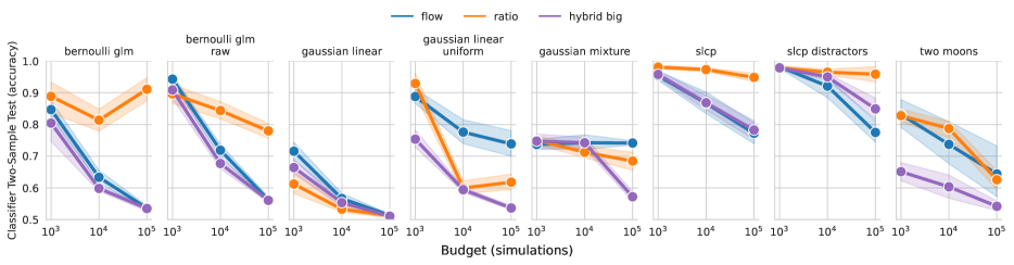
Figure 3: The C2ST accuracy and 95% confidence intervals are plotted versus simulation budget for three surrogate models on eight benchmark tasks. We estimate the exactness of the surrogate model against tractable posterior samples. Lower values indicate either a better fit, or limitations of the C2ST itself. The flow architecture trains a Normalized Density Surrogate Model that optimizes Equation 7 and is equivalent to npe. The ratio architecture trains the Posterior-to-Prior Energy-based Ratio Surrogate Model that optimizes Equation 8. Finally, the hybrid big architecture trains a Hybrid Surrogate Model that optimizes Equation 9.

It has become standard in the sbi literature to measure the exactness of the surrogate against a tractable posterior as a function of simulation budget, despite failing to represent the practitioner’s setting (Hermans et al., 2022). Lueckmann et al. (2021) collected ten priors and simulators, each with ten parameter-observation pairs and 10,000 samples from the corresponding likelihood-based posterior, to create the so-called Simulation-based Inference Benchmark. The parameters range between two- and ten-dimensional while the simulations range between two- and 100-dimensional. The benchmark measures the five-fold cross-validated Classifier Two-Sample Test (C2ST) Friedman (2003); Lopez-Paz & Oquab (2017) accuracy by comparing samples from the posterior and the surrogate at simulation budgets between $10^{3}$ and $10^{5}$ joint samples. Classification accuracies of 0.5 indicate that either the surrogate is indistinguishable from the posterior from the given samples, or that the classifier does not have the capacity to tell the distributions apart. p-values and E-values Pandeva et al. (2022) are not considered.

Experiments were done with a Neural Spline Flow (NSF)-based normalized density surrogate Durkan et al. (2019), a posterior-to-prior ratio-based surrogate, and a hybrid surrogate which trained a ratio against a Masked Autoregressive Flow (MAF)-based density estimator Papamakarios et al. (2017). Following Delaunoy et al. (2023), we appended an unconditional bijection from the final distribution layer to the prior support in all normalizing flows. We found that it increased training stability when the prior $p(\boldsymbol{\theta})$ was uniform.

Results

We report C2ST results across 8 tasks, all aforementioned models, and several architectures in Figure 3. We averaged over ten random seeds per plotted point to create the 95% confidence intervals with an approximately 76 node-day computational cost for all runs across all hyperparameters. Architecture and training details are in Appendix B, including Figure 4 that shows additional results for ratio big and hybrid that correspond to the same model, but with varied neural network hyperparameter choices. Additionally, for the hybrid models, we report the C2ST for samples from either the base distribution $b_{v}(\boldsymbol{\theta}\,|\,\boldsymbol{x})$ or the full hybrid model $\exp\rho_{w}(\boldsymbol{\theta},\boldsymbol{x})b_{v}(\boldsymbol{\theta}\,|\,\boldsymbol{x})$ in Figure 6. It diagnoses how much each component contributes to the overall surrogate.

The hybrid big model was generally more accurate than flow or ratio, although there were exceptions: In Gaussian Linear and SLCP Distractors the ratio or flow models were better. Ratio was very sensitive to neural network size and cannot be trusted to solve Gaussian Linear accurately with arbitrary neural network design. SLCP has a complex shape and may have benefited from using a Neural Spline Flow as the base distribution for hybrid big. Two Moons features extreme multi-modality allowing hybrid big to shine: The base distribution $b_{v}(\boldsymbol{\theta}\,|\,\boldsymbol{x})$ left a typical narrow tail connecting each moon, but the ratio $\exp\rho_{w}(\boldsymbol{\theta},\boldsymbol{x})$ erased this tail density. A visualization of an example surrogate and reference posterior can be found in Figure 5.

4 Conclusion

We proposed to use the Generalized KL-divergence, in expectation over $p(\boldsymbol{x})$, as an objective for sbi, connected it to npe, proposed estimating the posterior-to-prior ratio using this objective, and proposed a natural hybrid model class for sbi. We evaluated the exactness of fits empirically on eight benchmark problems at three simulation budgets, representing over two months of computation time. Our conclusion was that the increased flexibility of our objective and the hybrid model was generally beneficial in comparison to flow, i.e. npe, but especially for Two Moons that features a multi-modal posterior. Fitting the ratio alone, with our objective, was very sensitive to neural network hyperparameter choices, emphasizing the importance of the hybrid model.

In the hybrid model, one must choose a variational family for the base distribution $b_{v}(\boldsymbol{\theta}\,|\,\boldsymbol{x})$. The base distribution must be more tightly concentrated than the prior to see improvement in performance, while also covering the entire posterior mass. In scientific settings, a conditional normal distribution with mean and covariance estimated by neural networks should be effective in most situations (without long-tailed posteriors). For the benchmark, we choose MAF since it was flexible and unlikely to exclude posterior mass.

In Section 2 and our experiments, we used a single sample to estimate $\operatorname{\mathbb{E}}_{p(\boldsymbol{x})}\left[Z_{w}(\boldsymbol{x})\right]$. As a Monte Carlo estimate, it has a variance $\propto\frac{1}{N}$ where $N$ represents the number of samples in the estimate. The constant of proportionality may be very large, meaning that a single sample is insufficiently accurate. Investing the quantitative effect of the number of contrastive samples on learning has been left to future work, although we expect that it might have a significant effect for the ratio surrogate. A theoretical analysis of the variance of $\operatorname{\mathbb{E}}_{p(\boldsymbol{x})}\left[Z_{w}(\boldsymbol{x})\right]$ is offered in Federici et al. (2023) along with experiments in estimating the mutual information using a varied number of so-called “negative” samples.

A natural follow-up work would extend our method to the so-called sequential case, where we train the surrogate estimator in a sequence of rounds. In each round, simulation data is drawn such that the current posterior estimate focuses attention on $\boldsymbol{x}$ which are “close” to an observation-of-interest $\boldsymbol{x}_{o}$. We plan to use the flexibility of our objective by updating the sampling distribution $p_{n}(\boldsymbol{\theta},\boldsymbol{x})$ across $n$ rounds.

Broader impact

The primary application of sbi is to solve the inverse problem on observations using high-fidelity simulation data. The broader societal impact is therefore limited to which simulators are considered for application.

Since sbi does not rely on likelihoods, it can be challenging to determine whether surrogates are overfit and provide inaccurate certainty about estimated parameters. We emphasize rigorous statistical testing to confirm results from sbi to avoid drawing inaccurate conclusions.

Appendix A Generalized Kullback-Leibler Divergence Details

We continue directly from Section 2 with a formulation of Gibbs’ inequality as a Theorem. Since the Generalized KL-Divergence is a $\phi$-divergence, this is review for our specific divergence choice.

Theorem 1 (Gibbs’ inequality for the Generalized KL-Divergence).

We always have the inequality:

$$\operatorname{\textsc{GKL}}(p(\boldsymbol{\theta})\,\|\,q(\boldsymbol{\theta})) \geq 0.$$ (10)

Furthermore, the equality $\operatorname{\textsc{GKL}}(p(\boldsymbol{\theta})\,\|\,q(\boldsymbol{\theta}))=0$ holds if and only if $p(\boldsymbol{\theta})=q(\boldsymbol{\theta})$ for $p(\boldsymbol{\theta})$-almost-all points $\boldsymbol{\theta}$, in other words, if they are equal inside the support of $p(\boldsymbol{\theta})$.

Proof.

Consider the following function $\phi:\,(0,\infty)\to\mathbb{R}$ given by:

$$\phi(r) :=-\ln(r)+r-1,$$ (11)

with the additional setting $\phi(0):=\phi(\infty):=\infty$. It always holds that $\phi(r)\geq 0$, with equality if and only if $r=1$. So, for any non-negative measurable function $R\geq 0$ we have: $\int\phi(R(\boldsymbol{z}))\,p(\boldsymbol{z})\,d\boldsymbol{z}\geq 0$ with equality if and only if $R(\boldsymbol{z})=1$ $p(\boldsymbol{z})$-almost-surely. Our case follows from $\boldsymbol{z}=\boldsymbol{\theta}$, $R(\boldsymbol{z})=\frac{q(\boldsymbol{\theta})}{p(\boldsymbol{\theta})}$ and $p(\boldsymbol{z})=p(\boldsymbol{\theta})$. ∎

Remark 1.

1. The above equality holds for unnormalized probability distributions, not just up to normalizing constants.

2. For normalized probability distributions $p_{1}(\boldsymbol{\theta})$ and $p_{2}(\boldsymbol{\theta})$ we recover the classical KL-divergence:

   $$\operatorname{\textsc{GKL}}(p_{1}(\boldsymbol{\theta})\,\|\,p_{2}(\boldsymbol{\theta})) =\operatorname{\mathbb{E}}_{p_{1}(\boldsymbol{\theta})}\left[\ln\frac{p_{1}(\boldsymbol{\theta})}{p_{2}(\boldsymbol{\theta})}\right]=:\operatorname{\textsc{KL}}(p_{1}(\boldsymbol{\theta})\,\|\,p_{2}(\boldsymbol{\theta})).$$ (12)

   In this sense, the Generalized $\operatorname{\textsc{KL}}$-divergence is a real generalization of the classical $\operatorname{\textsc{KL}}$-divergence.

Our general Gibbs’ inequality now allows us to formulate a generalization of the classical minimal (relative) entropy principle (Kullback & Leibler, 1951; Shore & Johnson, 1980; Cover, 1999):

Principle (The principle of minimal Generalized KL-divergence).

Let $p(\boldsymbol{\theta})$ be an underlying “true,” given probability distribution that we want to approximate with a(n unnormalized) probability distribution $q(\boldsymbol{\theta})$ from a certain model class $\mathcal{F}$, expressing certain prior knowledge or constraints.

Then the principle of minimal Generalized KL-divergence expresses that one should choose that $q(\boldsymbol{\theta})$ from $\mathcal{F}$ that has minimal Generalized KL-divergence to $p(\boldsymbol{\theta})$, i.e. one should choose:

$$q^{*}(\boldsymbol{\theta})\in\operatorname*{arg\,min}_{q(\boldsymbol{\theta})\in\mathcal{F}}\operatorname{\textsc{GKL}}(p(\boldsymbol{\theta})\,\|\,q(\boldsymbol{\theta})).$$ (13)

Finally, we prove Equation 4:

$$\begin{aligned} Z_{p}\cdot\operatorname{\textsc{KL}}(p(\boldsymbol{\theta})/Z_{p}\,\|\,q(\boldsymbol{\theta})/Z_{q})&=Z_{p}\int\frac{p(\boldsymbol{\theta})}{Z_{p}}\ln\frac{p(\boldsymbol{\theta})/Z_{p}}{q(\boldsymbol{\theta})/Z_{q}}\,d\boldsymbol{\theta}\\ &=-\int p(\boldsymbol{\theta})\ln\frac{p(\boldsymbol{\theta})}{q(\boldsymbol{\theta})}\,d\boldsymbol{\theta}+Z_{p}\ln\frac{Z_{q}}{Z_{p}}\\ &\leq-\int p(\boldsymbol{\theta})\ln\frac{p(\boldsymbol{\theta})}{q(\boldsymbol{\theta})}\,d\boldsymbol{\theta}+Z_{p}\left(\frac{Z_{q}}{Z_{p}}-1\right)\\ &=-\int p(\boldsymbol{\theta})\ln\frac{p(\boldsymbol{\theta})}{q(\boldsymbol{\theta})}\,d\boldsymbol{\theta}+Z_{q}-Z_{p}\\ &=-\int p(\boldsymbol{\theta})\ln\frac{p(\boldsymbol{\theta})}{q(\boldsymbol{\theta})}\,d\boldsymbol{\theta}+\int q(\boldsymbol{\theta})\,d\boldsymbol{\theta}-\int p(\boldsymbol{\theta})\,d\boldsymbol{\theta}\\ &=-\int p(\boldsymbol{\theta})\left(\ln\frac{p(\boldsymbol{\theta})}{q(\boldsymbol{\theta})}+\frac{q(\boldsymbol{\theta})}{p(\boldsymbol{\theta})}-1\right)\,d\boldsymbol{\theta}\\ &=\operatorname{\textsc{GKL}}(p(\boldsymbol{\theta})\,\|\,q(\boldsymbol{\theta})).\end{aligned}$$ (14)

Appendix B Experimental Details

In this section we include more information about the tasks, hyperparameters that we chose, and a few more results.

B.1 Simulation-based Inference Benchmark Task Details

We provide a short summary of all of the inference tasks we consdiered from the sbi benchmark by Lueckmann et al. (2021).

• This task is a generalized linear model. The likelihood is Bernoulli distributed. The data is a 10-dimensional sufficient statistic from an 100-dimensional vector. The posterior is 10-dimensional with only one mode.

• This is the same task as above, but instead the entire 100-dimensional observation is shown to the inference method rather than the summary statistic.

• A simple task with a Gaussian distributed prior and a Gaussian likelihood over the mean. Both have a $\Sigma=0.1\cdot I$ covariance matrix. The posterior is also Gaussian. It is performed in 10-dimensions for the observations and parameters.

• This is the same as the task above, but instead the prior over the mean is a 10-dimensional uniform distribution from -1 to 1 in every dimension.

• This task occurs in the ABC literature often. Infer the common mean of a mixture of Gaussians where one has covariance matrix $\Sigma=1.0\cdot I$ and the other $\Sigma=0.01\cdot I$. It occurs in two dimensions.

• A task which has a very simple non-spherical Gaussian likelihood, but a complex posterior over the five parameters which, via a non-linear function, define the mean and covariance of the likelihood. There are five parameters each with a uniform prior from -3 to 3. The data is four-dimensional but we take two samples from it.

• This is the same as above but instead the data is concatenated with 92 dimensions of Gaussian noise.

• This task exhibits a crescent shape posterior with bi-modality–two of the attributes often used to stump mcmc samplers. Both the data and parameters are two dimensional. The prior is uniform from -1 to 1.

B.2 Hyperparameters

In this section we report the hyperparameters for each of our models in Table 1. AdamW is an optimizer introduced by Loshchilov & Hutter (2017). LWCR stands for Linear Warmup Cosine Annealing. NSF stands for Neural Spline Flow and MAF stands for Masked Autoregressive Flow.

Table 1: Hyperparameters

Model Name	flow	ratio	ratio big	hybrid	hybrid big
Batch size	16384	16384	16384	16384	16384
Embedding Net	ResNet			ResNet	ResNet
Embedding Net Hidden Dim	[64]			[64]	[64]
Embedding Net Activation	gelu			gelu	gelu
Embedding Net Normalization	Layer Norm			Layer Norm	Layer Norm
Flow	NSF			MAF	MAF
Flow Num Transforms	5			5	5
Flow Num Bins	8
Flow Hidden Dim	[64]			[64]	[64]
Flow Activation	relu			relu	relu
Ratio Estimator		ResNet	ResNet	ResNet	ResNet
Ratio Estimator Hidden Dim		[128]	[256, 256]	[128]	[256, 256]
Ratio Estimator Activation		gelu	gelu	gelu	gelu
Ratio Estimator Normalization		Layer Norm	Layer Norm	Layer Norm	Layer Norm
Optimizer	AdamW	AdamW	AdamW	AdamW	AdamW
Learning Rate	0.001	0.001	0.001	0.001	0.001
Weight Decay	0.001	0.001	0.001	0.001	0.001
amsgrad	True	True	True	True	True
LR Schedule	LWCA	LWCA	LWCA	LWCA	LWCA
LR Schedule Warmup Percent	0.100	0.100	0.100	0.100	0.100
LR Schedule Starting LR	1e-8	1e-8	1e-8	1e-8	1e-8
LR Schedule eta	1e-8	1e-8	1e-8	1e-8	1e-8
Early Stopping	True	True	True	True	True
Early Stop Minimum Delta	0.003	0.003	0.003	0.003	0.003
Early Stop Patience	322	322	322	322	322

B.3 Further Results

We present results from the ratio big and hybrid models, along with repeated presentation of previous results, in Figure 4. We break the hybrid model into parts and show results based on taking samples directly from the underlying normalized base distribution $b_{v}(\boldsymbol{\theta}\,|\,\boldsymbol{x})$ and compare that to samples from the full hybrid model $\exp\rho_{w}(\boldsymbol{\theta},\boldsymbol{x})b_{v}(\boldsymbol{\theta}\,|\,\boldsymbol{x})$. Qualitative results on a observation $\boldsymbol{x}_{9}$ from Two Moons is plotted in Figure 5, and quantitative results across tasks are plotted in Figure 6.

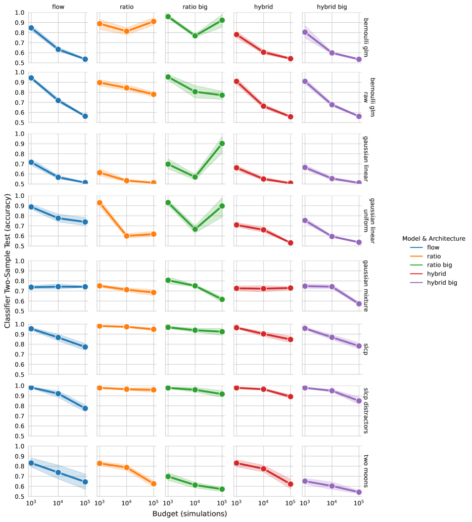
Figure 4: The C2ST accuracy and 95% confidence intervals are plotted versus simulation budget for five surrogate models on eight benchmark tasks. We estimate the exactness of the surrogate model against tractable posterior samples. Lower values indicate either a better fit, or limitations of the C2ST itself. Details about model hyperparameters can be found in Table 1.

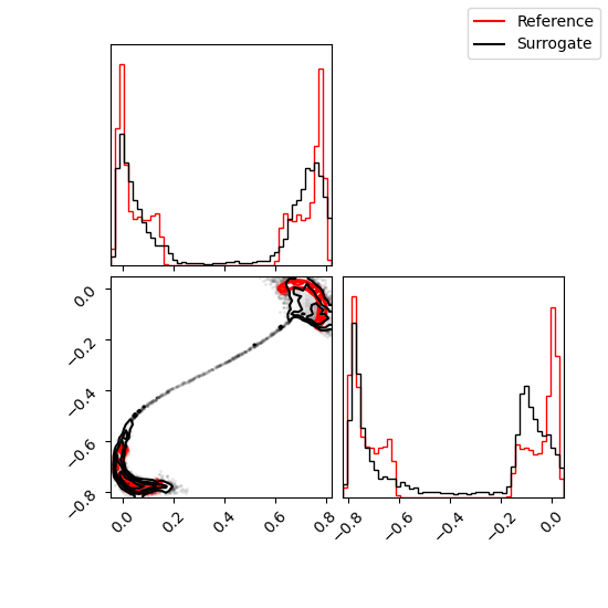
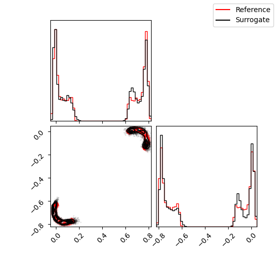
Figure 5: Two corner plots of the posterior and surrogate densities for Two Moons $\boldsymbol{x}_{9}$. In both figures, the same reference posterior is drawn in red. The black lines represent different parts of the same hybrid surrogate. On the left, the samples come from density estimator $b_{v}(\boldsymbol{\theta}\,|\,\boldsymbol{x})$. On the right, samples come from the full hybrid model $\exp\rho_{w}(\boldsymbol{\theta},\boldsymbol{x})b_{v}(\boldsymbol{\theta}\,|\,\boldsymbol{x})$. The ratio estimator improves the shape significantly.

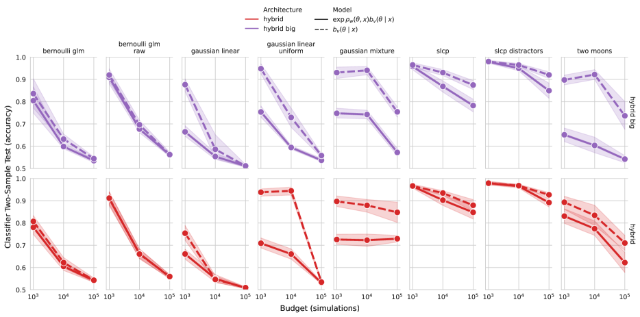
Figure 6: The C2ST accuracy and 95% confidence intervals are plotted versus simulation budget for two hybrid surrogate models on eight benchmark tasks. We estimate the exactness of the surrogate model against tractable posterior samples. The analysis was performed on samples from the same hybrid model, but the dotted line represents samples from only the normalized conditional density estimator $b_{v}(\boldsymbol{\theta}\,|\,\boldsymbol{x})$ while the solid line represents samples from the full hybrid surrogate $\exp\rho_{w}(\boldsymbol{\theta},\boldsymbol{x})b_{v}(\boldsymbol{\theta}\,|\,\boldsymbol{x})$. Lower values indicate either a better fit, or limitations of the C2ST itself. Details about model hyperparameters can be found in Table 1.

References

- Ali & Silvey (1966) Ali, S. M. and Silvey, S. D. A general class of coefficients of divergence of one distribution from another. Journal of the Royal Statistical Society: Series B (Methodological), 28(1):131–142, 1966.
- Alsing et al. (2018) Alsing, J., Wandelt, B., and Feeney, S. Massive optimal data compression and density estimation for scalable, likelihood-free inference in cosmology. Monthly Notices of the Royal Astronomical Society, 477(3):2874–2885, 2018.
- Alsing et al. (2019) Alsing, J., Charnock, T., Feeney, S., and Wandelt, B. Fast likelihood-free cosmology with neural density estimators and active learning. Monthly Notices of the Royal Astronomical Society, 488(3):4440–4458, 2019.
- Arbel et al. (2021) Arbel, M., Zhou, L., and Gretton, A. Generalized energy based models. In International Conference on Learning Representations, 2021. URL https://openreview.net/forum?id=0PtUPB9z6qK.
- Barber & Agakov (2003) Barber, D. and Agakov, F. The im algorithm: a variational approach to information maximization. In Proceedings of the 16th International Conference on Neural Information Processing Systems, pp. 201–208, 2003.
- Belghazi et al. (2018) Belghazi, M. I., Baratin, A., Rajeswar, S., Ozair, S., Bengio, Y., Courville, A., and Hjelm, R. D. Mine: mutual information neural estimation. arXiv preprint arXiv:1801.04062, 2018.
- Bhardwaj et al. (2023) Bhardwaj, U., Alvey, J., Miller, B. K., Nissanke, S., and Weniger, C. Peregrine: Sequential simulation-based inference for gravitational wave signals. arXiv preprint arXiv:2304.02035, 2023.
- Bishop (1994) Bishop, C. M. Mixture density networks. Technical Report, 1994.
- Cole et al. (2021) Cole, A., Miller, B. K., Witte, S. J., Cai, M. X., Grootes, M. W., Nattino, F., and Weniger, C. Fast and credible likelihood-free cosmology with truncated marginal neural ratio estimation. arXiv preprint arXiv:2111.08030, 2021.
- Cornish et al. (2020) Cornish, R., Caterini, A., Deligiannidis, G., and Doucet, A. Relaxing bijectivity constraints with continuously indexed normalising flows. In International conference on machine learning, pp. 2133–2143. PMLR, 2020.
- Cover (1999) Cover, T. M. Elements of information theory. John Wiley & Sons, 1999.
- Cranmer et al. (2020) Cranmer, K., Brehmer, J., and Louppe, G. The frontier of simulation-based inference. Proc. Natl. Acad. Sci. U. S. A., May 2020.
- Csiszár (1963) Csiszár, I. Eine informationstheoretische ungleichung und ihre anwendung auf den beweis der ergodizität von markoffschen ketten. In Publ. Math. Inst., volume 8, pp. 85–107. Hungar. Acad. Sci., 1963.
- Dalmasso et al. (2021) Dalmasso, N., Zhao, D., Izbicki, R., and Lee, A. B. Likelihood-free frequentist inference: Bridging classical statistics and machine learning in simulation and uncertainty quantification. arXiv preprint arXiv:2107.03920, 2021.
- Dax et al. (2021) Dax, M., Green, S. R., Gair, J., Macke, J. H., Buonanno, A., and Schölkopf, B. Real-time gravitational wave science with neural posterior estimation. Physical review letters, 127(24):241103, 2021.
- Delaunoy et al. (2023) Delaunoy, A., Miller, B. K., Forré, P., Weniger, C., and Louppe, G. Balancing simulation-based inference for conservative posteriors. arXiv preprint arXiv:2304.10978, 2023.
- Durkan et al. (2019) Durkan, C., Bekasov, A., Murray, I., and Papamakarios, G. Neural spline flows. Advances in neural information processing systems, 32, 2019.
- Federici et al. (2023) Federici, M., Ruhe, D., and Forré, P. On the effectiveness of hybrid mutual information estimation. arXiv preprint arXiv:2306.00608, 2023.
- Friedman (2003) Friedman, J. H. On multivariate goodness–of–fit and two–sample testing. STATISTICAL PROBLEMS IN PARTICLE PHYSICS, ASTROPHYSICS AND COSMOLOGY, pp. 311, 2003.
- Geffner et al. (2022) Geffner, T., Papamakarios, G., and Mnih, A. Score modeling for simulation-based inference. arXiv preprint arXiv:2209.14249, 2022.
- Glaser et al. (2022) Glaser, P., Arbel, M., Doucet, A., and Gretton, A. Maximum likelihood learning of energy-based models for simulation-based inference. arXiv preprint arXiv:2210.14756, 2022.
- Glöckler et al. (2021) Glöckler, M., Deistler, M., and Macke, J. H. Variational methods for simulation-based inference. In International Conference on Learning Representations, 2021.
- Gratton (2017) Gratton, S. Glass: A general likelihood approximate solution scheme. arXiv preprint arXiv:1708.08479, 2017.
- Greenberg et al. (2019) Greenberg, D., Nonnenmacher, M., and Macke, J. Automatic posterior transformation for likelihood-free inference. In International Conference on Machine Learning, pp. 2404–2414. PMLR, 2019.
- Hermans et al. (2020) Hermans, J., Begy, V., and Louppe, G. Likelihood-free mcmc with amortized approximate ratio estimators. In International Conference on Machine Learning, pp. 4239–4248. PMLR, 2020.
- Hermans et al. (2022) Hermans, J., Delaunoy, A., Rozet, F., Wehenkel, A., Begy, V., and Louppe, G. A crisis in simulation-based inference? beware, your posterior approximations can be unfaithful. Transactions on Machine Learning Research, 2022. ISSN 2835-8856. URL https://openreview.net/forum?id=LHAbHkt6Aq.
- Huang et al. (2018) Huang, C.-W., Krueger, D., Lacoste, A., and Courville, A. Neural autoregressive flows. In International Conference on Machine Learning, pp. 2078–2087. PMLR, 2018.
- Kong & Chaudhuri (2020) Kong, Z. and Chaudhuri, K. The expressive power of a class of normalizing flow models. In International conference on artificial intelligence and statistics, pp. 3599–3609. PMLR, 2020.
- Kullback & Leibler (1951) Kullback, S. and Leibler, R. A. On information and sufficiency. The annals of mathematical statistics, 22(1):79–86, 1951.
- Lemos et al. (2023) Lemos, P., Coogan, A., Hezaveh, Y., and Perreault-Levasseur, L. Sampling-based accuracy testing of posterior estimators for general inference. arXiv preprint arXiv:2302.03026, 2023.
- Liese & Vajda (2006) Liese, F. and Vajda, I. On divergences and informations in statistics and information theory. IEEE Transactions on Information Theory, 52(10):4394–4412, 2006.
- Linhart et al. (2022) Linhart, J., Gramfort, A., and Rodrigues, P. L. Validation diagnostics for sbi algorithms based on normalizing flows. arXiv preprint arXiv:2211.09602, 2022.
- Lopez-Paz & Oquab (2017) Lopez-Paz, D. and Oquab, M. Revisiting classifier two-sample tests. In International Conference on Learning Representations, 2017.
- Loshchilov & Hutter (2017) Loshchilov, I. and Hutter, F. Decoupled weight decay regularization. arXiv preprint arXiv:1711.05101, 2017.
- Lueckmann et al. (2017) Lueckmann, J.-M., Gonçalves, P. J., Bassetto, G., Öcal, K., Nonnenmacher, M., and Macke, J. H. Flexible statistical inference for mechanistic models of neural dynamics. In Proceedings of the 31st International Conference on Neural Information Processing Systems, pp. 1289–1299, 2017.
- Lueckmann et al. (2021) Lueckmann, J.-M., Boelts, J., Greenberg, D., Goncalves, P., and Macke, J. Benchmarking simulation-based inference. In Banerjee, A. and Fukumizu, K. (eds.), Proceedings of The 24th International Conference on Artificial Intelligence and Statistics, volume 130 of Proceedings of Machine Learning Research, pp. 343–351. PMLR, 13–15 Apr 2021. URL http://proceedings.mlr.press/v130/lueckmann21a.html.
- Masserano et al. (2022) Masserano, L., Dorigo, T., Izbicki, R., Kuusela, M., and Lee, A. B. Simulation-based inference with waldo: Perfectly calibrated confidence regions using any prediction or posterior estimation algorithm. arXiv preprint arXiv:2205.15680, 2022.
- Miller et al. (2021) Miller, B. K., Cole, A., Forré, P., Louppe, G., and Weniger, C. Truncated marginal neural ratio estimation. Advances in Neural Information Processing Systems, 34:129–143, 2021.
- Miller et al. (2022) Miller, B. K., Weniger, C., and Forré, P. Contrastive neural ratio estimation. Advances in Neural Information Processing Systems, 35:3262–3278, 2022.
- Nguyen et al. (2010) Nguyen, X., Wainwright, M. J., and Jordan, M. I. Estimating divergence functionals and the likelihood ratio by convex risk minimization. IEEE Transactions on Information Theory, 56(11):5847–5861, 2010.
- Nowozin et al. (2016) Nowozin, S., Cseke, B., and Tomioka, R. f-gan: Training generative neural samplers using variational divergence minimization. Advances in neural information processing systems, 29, 2016.
- Pacchiardi & Dutta (2022) Pacchiardi, L. and Dutta, R. Score matched neural exponential families for likelihood-free inference. J. Mach. Learn. Res., 23(38):1–71, 2022.
- Pandeva et al. (2022) Pandeva, T., Bakker, T., Naesseth, C. A., and Forré, P. E-valuating classifier two-sample tests. arXiv preprint arXiv:2210.13027, 2022.
- Papamakarios & Murray (2016) Papamakarios, G. and Murray, I. Fast -free inference of simulation models with bayesian conditional density estimation. Advances in neural information processing systems, 29, 2016.
- Papamakarios et al. (2017) Papamakarios, G., Pavlakou, T., and Murray, I. Masked autoregressive flow for density estimation. In Proceedings of the 31st International Conference on Neural Information Processing Systems, pp. 2335–2344, 2017.
- Papamakarios et al. (2019a) Papamakarios, G., Nalisnick, E., Rezende, D. J., Mohamed, S., and Lakshminarayanan, B. Normalizing flows for probabilistic modeling and inference. arXiv preprint arXiv:1912.02762, 2019a.
- Papamakarios et al. (2019b) Papamakarios, G., Sterratt, D., and Murray, I. Sequential neural likelihood: Fast likelihood-free inference with autoregressive flows. In The 22nd International Conference on Artificial Intelligence and Statistics, pp. 837–848. PMLR, 2019b.
- Poole et al. (2019) Poole, B., Ozair, S., Van Den Oord, A., Alemi, A., and Tucker, G. On variational bounds of mutual information. In International Conference on Machine Learning, pp. 5171–5180. PMLR, 2019.
- Ramesh et al. (2021) Ramesh, P., Lueckmann, J.-M., Boelts, J., Tejero-Cantero, Á., Greenberg, D. S., Goncalves, P. J., and Macke, J. H. Gatsbi: Generative adversarial training for simulation-based inference. In International Conference on Learning Representations, 2021.
- Rényi (1961) Rényi, A. On measures of entropy and information. In Proceedings of the Fourth Berkeley Symposium on Mathematical Statistics and Probability, Volume 1: Contributions to the Theory of Statistics, volume 4, pp. 547–562. University of California Press, 1961.
- Reyes-González & Torre (2023) Reyes-González, H. and Torre, R. Testing the boundaries: Normalizing flows for higher dimensional data sets. Journal of Physics: Conference Series, 2438(1):012155, feb 2023. doi: 10.1088/1742-6596/2438/1/012155. URL https://doi.org/10.1088%2F1742-6596%2F2438%2F1%2F012155.
- Rhodes et al. (2020) Rhodes, B., Xu, K., and Gutmann, M. U. Telescoping density-ratio estimation. Advances in neural information processing systems, 33:4905–4916, 2020.
- Salimans et al. (2016) Salimans, T., Goodfellow, I., Zaremba, W., Cheung, V., Radford, A., and Chen, X. Improved techniques for training gans. Advances in neural information processing systems, 29, 2016.
- Sharrock et al. (2022) Sharrock, L., Simons, J., Liu, S., and Beaumont, M. Sequential neural score estimation: Likelihood-free inference with conditional score based diffusion models. arXiv preprint arXiv:2210.04872, 2022.
- Shore & Johnson (1980) Shore, J. and Johnson, R. Axiomatic derivation of the principle of maximum entropy and the principle of minimum cross-entropy. IEEE Transactions on Information Theory, 26(1):26–37, 1980. doi: 10.1109/TIT.1980.1056144.
- Sisson et al. (2018) Sisson, S. A., Fan, Y., and Beaumont, M. Handbook of approximate Bayesian computation. CRC Press, 2018.
- Song & Kingma (2021) Song, Y. and Kingma, D. P. How to train your energy-based models. arXiv preprint arXiv:2101.03288, 2021.
- Talts et al. (2018) Talts, S., Betancourt, M., Simpson, D., Vehtari, A., and Gelman, A. Validating bayesian inference algorithms with simulation-based calibration. arXiv preprint arXiv:1804.06788, 2018.
- Thomas et al. (2016) Thomas, O., Dutta, R., Corander, J., Kaski, S., Gutmann, M. U., et al. Likelihood-free inference by ratio estimation. Bayesian Analysis, 2016.
- Tran et al. (2017) Tran, D., Ranganath, R., and Blei, D. M. Hierarchical implicit models and likelihood-free variational inference. arXiv preprint arXiv:1702.08896, 2017.
- Wood (2010) Wood, S. N. Statistical inference for noisy nonlinear ecological dynamic systems. Nature, 466(7310):1102–1104, 2010.
- Zhao et al. (2021) Zhao, D., Dalmasso, N., Izbicki, R., and Lee, A. B. Diagnostics for conditional density models and bayesian inference algorithms. In Uncertainty in Artificial Intelligence, pp. 1830–1840. PMLR, 2021.