Discrete, compositional, and symbolic representations through attractor dynamics

Abstract

Compositionality is an important feature of discrete symbolic systems, such as language and programs, as it enables them to have infinite capacity despite a finite symbol set. It serves as a useful abstraction for reasoning in both cognitive science and in AI, yet the interface between continuous and symbolic processing is often imposed by fiat at the algorithmic level, such as by means of quantization or a softmax sampling step. In this work, we explore how discretization could be implemented in a more neurally plausible manner through the modeling of attractor dynamics that partition the continuous representation space into basins that correspond to sequences of symbols. Building on established work in attractor networks and introducing novel training methods, we show that imposing structure in the symbolic space can produce compositionality in the attractor-supported representation space of rich sensory inputs. Lastly, we argue that our model exhibits the process of an information bottleneck that is thought to play a role in conscious experience, decomposing the rich information of a sensory input into stable components encoding symbolic information.

1 Introduction

The language of thought hypothesis posits that human thought is symbolic and compositional, allowing us to construct a large number of complex representations by recombining a relatively small set of simple concepts [1, 2, 3, 4, 5]. For instance, human behavior and neural data on a set of working memory tasks can potentially be explained by a symbolic and compositional model in which stimuli are represented using the shortest program that reconstructs them [6]. However, while symbolic manipulation is a useful construct at the cognitive level [7], its implementation [8] at the neuronal level is almost certainly continuous and distributed [9]. Although deep learning has helped bridge the gap by incorporating inductive biases for discreteness in representations (e.g., [10, 11]) and symbolic processing [12, 13, 14, 15, 16, 17, 18, 19], these models explicitly assume discretization by means of discrete actions and the pre-allocation of neural modules [20], thereby demonstrating the strengths of neuro-symbolic algorithms but leaving open several implementation questions, notably in how discretization occurs.

Our work seeks to close this gap further by building on theoretical work by Ji et al. [21] that conceptualizes discretization through a dynamical system with attractor basins that partition a high-dimensional continuous space into discrete regions. Attractor networks and attractor-based representations are not new, yet their use in a compositional and symbolic setting remain relatively unexplored. Intuitively, the model should learn to sample trajectories to multiple attractors for a given input proportional to how well their corresponding sentence representations encode the input. However, defining these properties as a differentiable objective function for a neural network model is difficult since initially, there is no grounded meaning in the model’s internal language and thus the target density is not known. Moreover, the learned symbolic representations should represent semantic attributes of the inputs such that they form a compositional code of meaningful primitives rather than arbitrary mappings. We overcome this limitation by using a generative flow network (GFN) [22] which allows us to specify the desired distribution using an unnormalized target function and the GFN expectation-maximization algorithm (GFN-EM) [23] to learn the mapping between the attractors and their symbolic representations. We demonstrate that not only is such a dynamical system learnable using a neural network, but that the learned attractors also adopt compositional structure to efficiently encode information using sequences of symbols.

We summarize our contributions as the following:

1. A model that bridges high-dimensional, continuous, distributed patterns of neural activity and discrete compositional “thoughts” at the implementation level using attractor dynamics.

2. A method for learning an emergent compositional language that encodes rich sensory information using the generative flow network expectation-maximization algorithm (GFN-EM) [23].

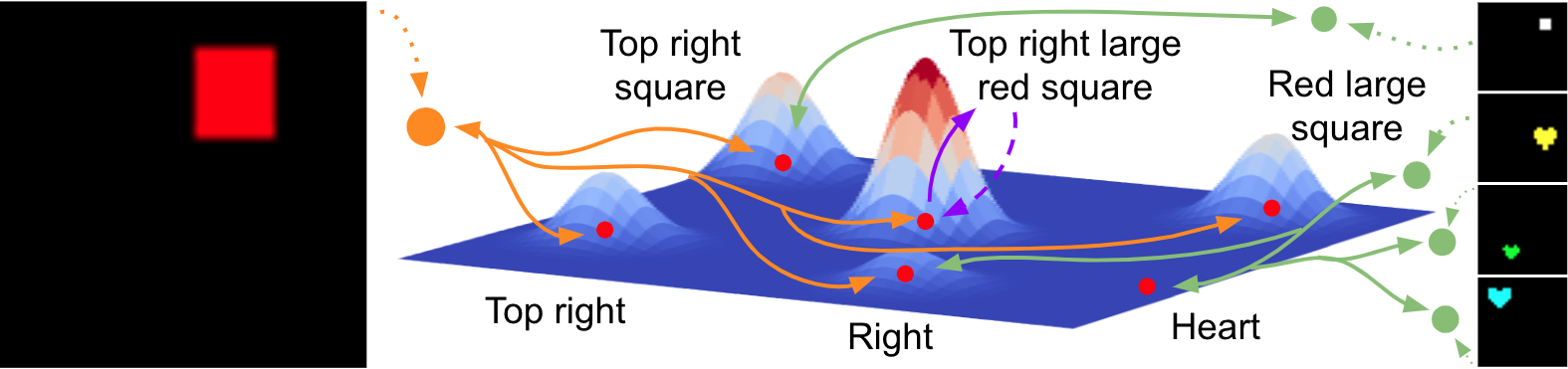
Figure 1: Model concept. The density landscape is the terminal distribution of $z_{T}$ given the input on the left, where the height of each mode is proportional to how well the corresponding sentence represents it. The orange dotted line shows the initial encoding using $P(z_{0}|x)$ and the solid lines show sample trajectories by following the stochastic dynamics $P(z_{t+1}|z_{t})$. The modes correspond to symbol sequences $w$, and the red points at the modes indicate the sentence embeddings $\hat{z}_{w}$, which are related to the sentences via the discretizer ($P(w|z,x)$) and embedding ($\hat{z}_{w}$) functions, represented using the solid and dashed purple lines. Green lines indicate trajectories that originate from other inputs. Trajectories are shown using bi-directional arrows, representing the forward and backward policies learned by the model.

2 Methods

We construct our model as a dynamical system defined by a continuous stochastic policy $P_{\theta}(z_{t+1}|z_{t},x)$ over time $t=1..T$ that begins at some latent representation $z_{0}\sim P_{\theta}(z_{0}|x)$ of an input $x$ and terminates at a point $z_{T}$, which is expected to be near an attractor $\hat{z}_{w}$ corresponding to some discrete token sequence $w$. The policy is a conditional Gaussian distribution with parameters output by a neural network, i.e., a discretized neural stochastic differential equation [24].

The relationship between an attractor point $\hat{z}$ in continuous space and its tokenized form is represented using a stochastic discretizer function $d_{\theta}:z\mapsto w$ and a deterministic embedding function $e_{\phi}:w\mapsto\hat{z}_{w}$. The unfolded trajectory $z_{0}\rightsquigarrow z_{T}$ from the initial encoding to the attractor point models the continuous dynamics that underlie the discretization of rich information to compositional and stable thoughts. Thus, the model is trained to learn a terminal distribution $P(z_{T}|x)$ such that $z_{T}$ clusters around the attractor basin $\hat{z}$ proportionally to how well the attractor represents $x$.

Formally, our aim is to learn a marginal distribution $P(z_{T},w|x)$ over the final point of the trajectory $z_{T}$ and its discretization $w$ such that both are sampled proportionally to the reward function $R_{\phi}(z_{T},w;x)$ in Eq. 1 – a product model that combines a similarity/reconstruction measure $s_{\phi}(x,\hat{z}_{w})$, the distance between $z$ and the attractor point $\hat{z}_{w}$, and a prior $P_{\phi}(w)$ over the token sequence $w$.

$$P(z_{T},w\mid x)\propto R_{\phi}(z_{T},w,x)=s_{\phi}(x,\hat{z}_{w})\cdot\mathcal{N}(z_{T}\mid\hat{z}_{w},\epsilon^{2})\cdot P_{\phi}(w)$$ (1)

We train our model as a continuous generative flow network (GFN) [22, 25]: a method for learning a generative model that samples a trajectory of states such that the distribution of terminal states is proportional to an unnormalized target density. The training procedure alternates steps in an expectation-maximization (EM) loop [23] in which the dynamics model serves as a posterior estimator:

• The E-step optimizes the sampling policy, consisting of the initial embedding $P_{\theta}(z_{0}|x)$, the forward dynamics $P_{\theta}(z_{t+1}|z_{t},x)$, and the discretizer $d_{\theta}(w|z_{T},x)$, together with auxiliary objects for GFN optimization.

• The M-step optimizes the objects involved in the reward – $s_{\phi}(x,\hat{z}_{w})$, the attractor embeddings $\hat{z}_{w}$, and the prior $P_{\phi}(w)$ – so as to maximize the log-reward $\log R(z_{T},w,x)$ on pairs $z_{T},w$ drawn from the dynamics model learnt in the E-step. It also optimizes a reconstruction model $P_{\phi}(x|z_{0})$ that promotes high mutual information between $x$ and the initial point of the dynamics $z_{0}$.

Details of the GFN training objectives and the the sampling procedure are given in Appendix A and C respectively.

The forward dynamics and discretizer are conditioned on the input $x$. However, to decouple the neural dynamics model from dependence on the input $x$, we train a separate marginalized policy $P_{\theta}(z_{t+1}|z_{t})$ by maximizing the log-likelihood of sample trajectories drawn from $P_{\theta}(z_{t+1}|z_{t},x)$. This post hoc marginalization step is performed once, after the input-dependent model has been fully trained.

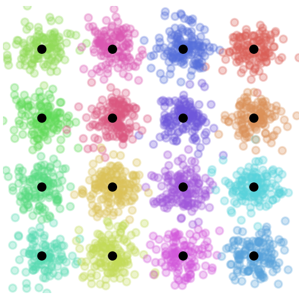
(a)

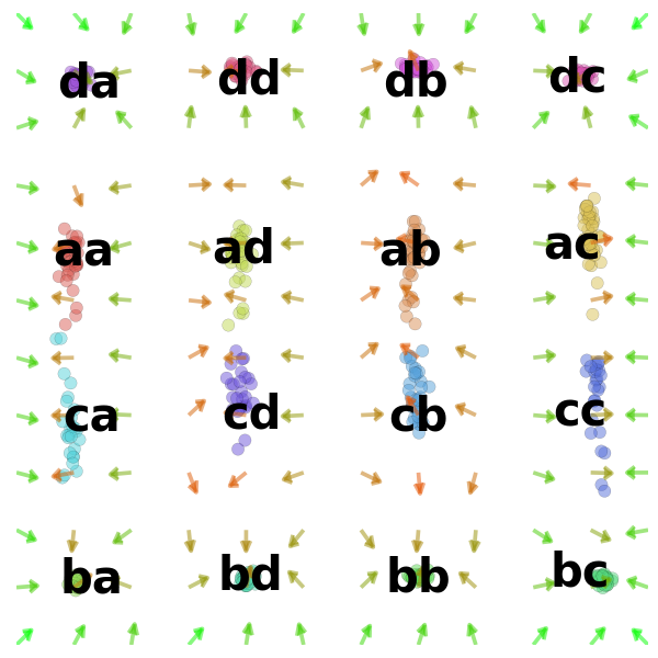
(b)

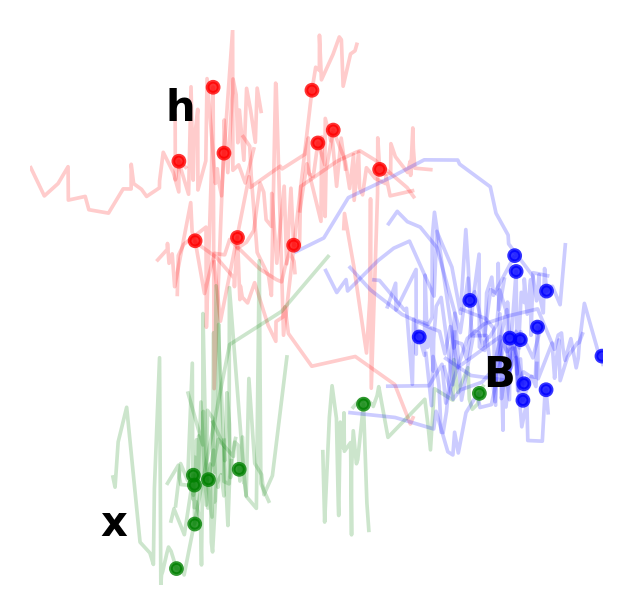
(c)

(d)

Figure 2: (a) The Gaussians dataset. Each point is colored according to the Gaussian it was sampled from. (b) The vector field, sentence embeddings, and terminal distribution of a model trained on the Gaussians task. (c) PCA of sample trajectories from the dSprites model using red, green, and blue images that terminated at attractors with sentences containing h, x, or B, which encode red, green, and blue respectively. (d) Left: sample sentences from the dSprites model using the red square input in Figure 1 and decoded images from their corresponding attractors. Right: averaged pixels of inputs with sample trajectories terminating at attractors where the sentences contain tokens h, o, or v.

3 Experiments

3.1 Grid of Gaussians

As an initial validation of our approach, we begin with a simple task where the inputs are generated from a mixture of 2-dimensional Gaussian distributions with component means in a $4\times 4$ grid [23] (Figure 2) where we can intuitively expect attractors to emerge at the center of each Gaussian. In this simplified setup, we let $z_{0}:=x$ (therefore $P(z_{0}|x)$, $P(x|z_{0})$, and $\mathcal{L}_{z_{0}}$ are not used) and use a distance based similarity measure $s(x,\hat{z}_{w})=\mathcal{N}(x|\hat{z}_{w},\epsilon^{2})$ with a fixed $\epsilon=.04$. Since there are $4\times 4$ Gaussians, we use length-2 token sequences with 4 possible tokens in each position.

Prior to training, the sentence embeddings are randomly positioned without any resemblance of compositionality or disentanglement. After training, however, the sentence embeddings settle to the center of each Gaussian that generated the dataset with contractive dynamics converging around the embedding points. Compositional syntax and semantics also emerge in the sentences that represent the attractor points, where the first token represents the row and the second token represents the column for the model shown in Figure 2. Incidentally, the meaning of the tokens are also tied to their positions in the sentence.

3.2 dSprites

To evaluate our model on a more complex task, we use the dSprites [26] dataset which consists of synthetic images that contain a single shape of various sizes in various positions. For our experiment, we colorized the dataset and simplified some features so that each input has one of 7 colors, 3 shapes, 6 sizes, and $5\times 5$ $(X,Y)$ coordinates. We allowed sentences with up to 5 tokens and a vocabulary size of 7 tokens per position.

Unlike in the Gaussians dataset, $z_{0}$ must be learned, without any guarantees that it would initially be disentangled or compositional. Moreover, the training objective for the attractive dynamics only encourages the model to use the existing sentence embeddings $\hat{z}_{w}$, allowing discretization to emerge but not necessarily compositional structure. Therefore, to induce compositionality, we require additional inductive biases over the structure of attractors, which we impose by maximizing the pointwise mutual information between $x$ and the sentence $w$ that maps to the attractor.

We once again use the GFN-EM algorithm to learn a compositional code for $X$ by using a conditional-VAE (CVAE) [27] for the similarity measure $s_{\phi}(x,z)$, where the encoder $P_{\phi}(\zeta|x,z)$ and decoder $P_{\phi}(x|\zeta,z)$ are conditioned on $z$. Intuitively, when applied to sentence representations, $\zeta$ represents information about $x$ that is not encoded in the sentence vector $\hat{z}_{w}$. However, the CVAE is liable to learn to reconstruct $x$ for any $w$, even when $w$ has incomplete or even incorrect information, by encoding the entire informational context of $x$ in $\zeta$. To minimize over-dependence on $\zeta$, we regularize the $s_{\phi}$ when training the discretizer $d_{\theta}$ using the KL-divergence between $P_{\phi}(\zeta|x,z)$ and $P(\zeta|z)$ = $\mathcal{N}(0,1)$, effectively penalizing the model for sampling $w$’s based the ineffable content, measured as on the number of additional bits of information that are needed to reconstruct $x$ [21].

$$\log s_{\phi}(x,z)=\log P_{\phi}(x|\zeta,z)+D_{\text{KL}}(P_{\phi}(\zeta|x,z)\ \|\ P(\zeta|w)=\mathcal{N}(0,1))$$ (2)

The trained model exhibits high compositionality and moderate disentanglement. Figure 2d shows samples drawn from the red square composed of tokens that represent red hues (‘h’), the right region (‘o’), and the top region (‘v’). To measure compositionality, we trained a linear decoder that takes a length-5 token sequence as a bag-of-words 5-hot vector and outputs to a probability distribution over the possible values of each feature. Because the contribution from each token is strictly additive, this decoder would only be able to predict accurately if the emergent language is compositional. We find that the position and individual RGB values of inputs can be linearly decoded with high accuracy, but not shape and scale, though even these are above chance (Table 1).

As a baseline, we performed principal component analysis (PCA) on the images to reduce their dimensions to 5 principal components, randomly projected these components to 35 dimensions, and binarized the dimensions by setting the 5 dimensions with the highest magnitude to 1 and all others to 0 to produce a 5-hot vector. This produces a length-5 discrete code with the same structure as the sentences sampled by our model. We also trained a zero-step model where we removed the dynamics module and conditioned the discretization directly on $z_{0}$. While the attractor model results in a higher accuracy than the PCA baseline, the zero-step model does better still, suggesting that there remains a gap in how well the attractor dynamics model can learn compositional code.

Table 1: Prediction accuracy of linear classifiers on a held-out set of dSprites images and their features. PCA results indicate top accuracy out of 100 random projections.

	X	Y	Shape	Scale	Color	R	G	B
Chance	20.0	20.0	33.3	16.7	14.3	50.0	50.0	50.0
PCA (max)	97.1	99.4	48.6	27.9	14.3	55.6	64.4	63.2
0 steps	95.4	94.2	88.7	40.2	92.9	94.1	98.1	98.6
Attractors	98.1	98.8	56.0	43.1	69.2	91.9	85.8	84.5

4 Discussion

The model we introduce in this paper builds on the theoretic advancements toward neurally plausible implementation of symbolic thought using attractor dynamics that partitions the space into discrete basins as proposed in Ji et al. [21]. The trajectory from the initial latent representation of the input to an attractor represents the loss of ineffable information, such that the resulting representation at the end of the trajectory is stable and resembles a symbolic entity, despite having arisen from distributed neural dynamics. Moreover, it also provides a way to measure this decomposition of the input’s informational content into its ineffable and effable components using the additional information provided by the input that is not contained in the symbolic representation.

We also show how properties of language can provide the inductive bias for learning compositional codes that represent rich, sensory information. However, a key limitation in our approach is that although the final resulting model successfully implements discretization from dynamics alone, the training method still relies on an explicit discretizer. Nevertheless, we view language as an important informational bottleneck that encourages the emergence of compositionality and enables the expressivity of reasoning and thought, and we hope to explore in future work how these explicit forms of discretization may be relaxed during training while retaining their useful inductive biases.

Appendix A GFlowNet Training Objective

The objective we use, detailed balance with forward-looking flow parametrization (FL-DB) [22, 28], requires optimizing several auxiliary objects: an estimate of the backward dynamics $P_{\theta}^{\leftarrow}(z_{t}|z_{t+1},t+1,x)$ and a ‘forward-looking flow’ model $g_{\theta}(z_{t},x,t)$ constrained to equal 0 when $t=T$. The forward and backward dynamics models are conditional Gaussian distributions with means and variances predicted by a neural network, so sampling of the policy is equivalent to Euler-Maruyama simulation of a stochastic differential equation. (Note that the forward dynamics are time-independent.) The FL-DB objective for a trajectory $z_{0}\rightsquigarrow z_{T}$, with symbol sequences $w_{i}$ sampled from each $z_{i}$, is:

$$\mathcal{L}_{\rm traj}=\sum\limits_{t=0}^{T-1}\left(\log\left(\dfrac{g_{\theta}(z_{t},x,t)}{g_{\theta}(z_{t+1},x,t+1)}\dfrac{R_{\phi}(z_{t},w_{t},x)}{R_{\phi}(z_{t+1},w_{t+1},x)}\dfrac{d_{\theta}(w_{t+1}|z_{t+1},x)}{d_{\theta}(w_{t}|z_{t},x)}\dfrac{P_{\theta}(z_{t+1}|z_{t},x)}{P_{\theta}^{\leftarrow}(z_{t}|z_{t+1},x)}\right)\right)^{2}$$ (3)

Although this objective is sufficient to train the model, jointly learning the dynamics and the discretizer can be difficult in practice. To improve training efficiency, the discretizer can be optimized separately by minimizing Eq. 4 with respect to the discretizer parameters and a learned estimator $F_{\theta}(z,x)$ and interweaving the updates between the dynamics and discretizer models. We note that although we define the discretization function as a distribution for the purposes of the GFN objective, its probability mass collapses to a single token sequence as $z$ approaches $\hat{z}_{w}$, becoming effectively a deterministic mapping.

$$\mathcal{L}_{\rm disc}=\left(\log\dfrac{d_{\theta}(z,x)d_{\theta}(w|z,x)}{R_{\phi}(z,w;x)}\right)^{2}$$ (4)

A significant challenge in training is that the reward penalizes based on distance from the sentence embedding at every point along the trajectory. Consequently, when there are two sentences that are equally representative of an input, the model will favor exploring the closer embedding and be slow to learn the more distant embedding as an attractor. Therefore, while the model can in theory learn to sample both modes with equal probability given sufficient training, this may take a very long time in practice. One possibility to accelerate training is to train the discretizer with its reward independent of $x$, such that $R_{\phi}(w;x)$ only measures how well $w$ encodes $x$ without considering the distance between $z$ and $\hat{z}_{w}$. The reward $R_{\phi}(z,w,x)$ is kept as is in $\mathcal{L}_{\text{traj}}$ so that the dynamics are still encouraged to move closer to the sentence embeddings.

The placement of the initial latent $z_{0}$ is trained using Eq. 5 by treating the flow at the start of the trajectory as the reward, weighted by the variational autoencoder (VAE) objective [29] to encourage mutual information between $z_{0}$ and $x$.

$$\mathcal{L}_{\rm init}=\left(\log\dfrac{F_{\theta}(x)P_{\theta}(z_{0}|x)}{P(z_{0})P_{\phi}(x|z_{0})F_{\theta}(z_{0},x,t=0)}\right)^{2}$$ (5)

Appendix B Training Details

In both experiments, we use a multi-layer perceptron (MLP) for the dynamics models that outputs the means and standard deviations of a Gaussian to sample the next step in the trajectory. We also use MLPs for the discretizer models $d_{\theta}$, where given $z$, the model simultaneously outputs $P(w_{i}|z)$ for each position $i$ in the token sequence. In the Gaussians task, the model always chooses between 4 tokens for both token positions, but we allow variable-length sequences in the dSprites task using a null token. We use a recurrent network for the embedding model $e_{\phi}:w\mapsto\hat{z}$ in the Gaussians task, where the memory vector is initialized as a projection of $z$, and the output vector after reading all $w_{i}$ is used as $\hat{z}_{w}$. In the dSprites task, we use an MLP for $e_{\phi}$. For simplicity, we use a uniform prior in both experiments.

We use a fixed $\epsilon$ in computing the distance measure $\mathcal{N}(z\mid\hat{z}_{w},\epsilon^{2})$. In the Gaussians task, we use .04, the same as used in the similarity measure $s(x,\hat{z}_{w})$. For the dSprites task, due to the high dimensionality of the latent space, we tune $\epsilon$ by pre-training a VAE to learn $P(\gamma\mid w)=\mathcal{N}(\gamma\mid\hat{z}_{w},\epsilon^{2})$ and $P(w\mid\gamma)$ with a single $\epsilon$ value for the whole model.

To accelerate training and help prevent modal collapse, we initialize the dSprites model with pretraining. First, rather than starting with attractors determined by a randomly initialized neural network that would place all attractors near the origin, we take the $\hat{z}_{w}$ learned by the VAE used to tune $\epsilon$. Second, learning $P_{\theta}(z_{0}\mid x)$ and $P_{\phi}(x\mid z_{0})$ can be challenging using the GFlowNet objective alone since the gradient is not passed through end-to-end, and so we pre-train these functions using the VAE objective instead. We note that $P_{\theta}(z_{0}\mid x)$ learned as a standard VAE is unlikely to produce compositional representations, and were not observed to do so in any of our experiments.

Appendix C Sampling

Given a fully trained model, we enumerate some of the possible ways to sample from the model. The steps below assume the model was trained on the dSprites dataset, where $z_{0}$ is a latent representation of $x$.

1. $P(z_{0},...,z_{T}\mid x)$: To sample a trajectory from an image, first sample $z_{0}\sim P(z_{0}\mid x)$ to get the initial encoding of the input. We then iteratively sample $z_{t+1}\sim P(z_{t+1}\mid z_{t})$ if using the marginalized model or $z_{t+1}\sim P(z_{t+1}\mid z_{t},x)$ using the input-dependent model.

2. $d_{\theta}(w\mid x)$: To sample a sentence from an image, first sample the trajectory $(z_{0},...,z_{T})$ using the above procedure, then sample $d_{\theta}(w\mid z_{T},x)$. If $z_{T}$ is sufficiently close to $\hat{z}_{w}$, then $d_{\theta}(w\mid z_{T},x)$ will be almost deterministic.

3. $P(x\mid w)$: To sample an image from a sentence, map $w$ to $\hat{z}_{w}$ using the embedding function, then use the auxiliary backward dynamics $P_{\theta}^{\leftarrow}(z_{t}|z_{t+1},t+1,x)$ starting from $\hat{z}_{w}$ for $T$ steps to get $(z_{0},...,z_{T-1},\hat{z}_{w})$. Use the reconstruction model $P_{\theta}(x\mid z_{0})$ to map $z_{0}$ into the input space.

References

- [1] Jerry A Fodor. The language of thought. Crowell Press, 1975.
- [2] Noah D Goodman, Joshua B Tenenbaum, and Tobias Gerstenberg. Concepts in a probabilistic language of thought. Technical report, Center for Brains, Minds and Machines (CBMM), 2014.
- [3] Brenden M. Lake, Tomer D. Ullman, Joshua B. Tenenbaum, and Samuel J. Gershman. Building machines that learn and think like people. Behavioral and Brain Sciences, 40, 2017.
- [4] Yoshua Bengio. The consciousness prior. arXiv preprint arXiv:1709.08568, 2019.
- [5] Anirudh Goyal and Yoshua Bengio. Inductive biases for deep learning of higher-level cognition. Proceedings of the Royal Society A, 478(2266):20210068, 2022.
- [6] Stanislas Dehaene, Fosca Al Roumi, Yair Lakretz, Samuel Planton, and Mathias Sablé-Meyer. Symbols and mental programs: a hypothesis about human singularity. Trends in Cognitive Sciences, 2022.
- [7] Jerry A Fodor and Zenon W Pylyshyn. Connectionism and cognitive architecture: A critical analysis. Cognition, 28(1-2):3–71, 1988.
- [8] David Marr. Vision: A computational investigation into the human representation and processing of visual information, 1982.
- [9] James L McClelland. Emergence in cognitive science. Topics in cognitive science, 2(4):751–770, 2010.
- [10] Aäron van den Oord, Oriol Vinyals, and Koray Kavukcuoglu. Neural discrete representation learning. Neural Information Processing Systems (NIPS), 2017.
- [11] Samuel Lavoie, Christos Tsirigotis, Max Schwarzer, Ankit Vani, Michael Noukhovitch, Kenji Kawaguchi, and Aaron Courville. Simplicial embeddings in self-supervised learning and downstream classification. International Conference on Learning Representations (ICLR), 2023.
- [12] Lionel Wong, Gabriel Grand, Alexander K. Lew, Noah D. Goodman, Vikash K. Mansinghka, Jacob Andreas, and Joshua B. Tenenbaum. From word models to world models: Translating from natural language to the probabilistic language of thought. arXiv preprint arXiv:2306.12672, 2023.
- [13] Thomas Pierrot, Nicolas Perrin, Feryal Behbahani, Alexandre Laterre, Olivier Sigaud, Karim Beguir, and Nando de Freitas. Learning compositional neural programs for continuous control. arXiv preprint arXiv:2007.13363, 2021.
- [14] Gautam Singh, Yeongbin Kim, and Sungjin Ahn. Neural systematic binder. International Conference on Learning Representations, 2023.
- [15] Kevin Ellis, Catherine Wong, Maxwell Nye, Mathias Sablé-Meyer, Lucas Morales, Luke Hewitt, Luc Cary, Armando Solar-Lezama, and Joshua B. Tenenbaum. DreamCoder: Bootstrapping inductive program synthesis with wake-sleep library learning. Programming Language Design and Implementation, 2021.
- [16] Anirudh Goyal, Aniket Didolkar, Nan Rosemary Ke, Charles Blundell, Philippe Beaudoin, Nicolas Heess, Michael Mozer, and Yoshua Bengio. Neural production systems: Learning rule-governed visual dynamics. Neural Information Processing Systems (NeurIPS), 2021.
- [17] Anirudh Goyal, Alex Lamb, Jordan Hoffmann, Shagun Sodhani, Sergey Levine, Yoshua Bengio, and Bernhard Schölkopf. Recurrent independent mechanisms. International Conference on Learning Representations (ICLR), 2021.
- [18] Anirudh Goyal, Alex Lamb, Phanideep Gampa, Philippe Beaudoin, Sergey Levine, Charles Blundell, Yoshua Bengio, and Michael Mozer. Object files and schemata: Factorizing declarative and procedural knowledge in dynamical systems. International Conference on Learning Representations (ICLR), 2021.
- [19] Anirudh Goyal, Aniket Didolkar, Alex Lamb, Kartikeya Badola, Nan Rosemary Ke, Nasim Rahaman, Jonathan Binas, Charles Blundell, Michael Mozer, and Yoshua Bengio. Coordination among neural modules through a shared global workspace. International Conference on Learning Representations (ICLR), 2022.
- [20] Sarthak Mittal, Yoshua Bengio, and Guillaume Lajoie. Is a modular architecture enough? Neural Information Processing Systems (NeurIPS), 2022.
- [21] Xu Ji, Eric Elmoznino, George Deane, Axel Constant, Guillaume Dumas, Guillaume Lajoie, Jonathan Simon, and Yoshua Bengio. Sources of richness and ineffability for phenomenally conscious states. arXiv preprint arXiv:2302.06403, 2023.
- [22] Yoshua Bengio, Salem Lahlou, Tristan Deleu, Edward J. Hu, Mo Tiwari, and Emmanuel Bengio. Gflownet foundations. Journal of Machine Learning Research, 24(210):1–55, 2023.
- [23] Edward J Hu, Nikolay Malkin, Moksh Jain, Katie Everett, Alexandros Graikos, and Yoshua Bengio. GFlowNet-EM for learning compositional latent variable models. International Conference on Machine Learning (ICML), 2023.
- [24] Belinda Tzen and Maxim Raginsky. Neural stochastic differential equations: Deep latent Gaussian models in the diffusion limit. arXiv preprint arXiv:1905.09883, 2019.
- [25] Salem Lahlou, Tristan Deleu, Pablo Lemos, Dinghuai Zhang, Alexandra Volokhova, Alex Hernández-García, Léna Néhale Ezzine, Yoshua Bengio, and Nikolay Malkin. A theory of continuous generative flow networks. International Conference on Machine Learning (ICML), 2023.
- [26] Loic Matthey, Irina Higgins, Demis Hassabis, and Alexander Lerchner. dsprites: Disentanglement testing sprites dataset. https://github.com/deepmind/dsprites-dataset/, 2017.
- [27] Kihyuk Sohn, Honglak Lee, and Xinchen Yan. Learning structured output representation using deep conditional generative models. Neural Information Processing Systems (NIPS), 2015.
- [28] Ling Pan, Nikolay Malkin, Dinghuai Zhang, and Yoshua Bengio. Better training of GFlowNets with local credit and incomplete trajectories. International Conference on Machine Learning (ICML), 2023.
- [29] Diederik P. Kingma and Max Welling. Auto-encoding variational Bayes. International Conference on Learning Representations (ICLR), 2014.