Energy-Guided Continuous Entropic Barycenter Estimation for General Costs

Abstract

Optimal transport (OT) barycenters are a mathematically grounded way of averaging probability distributions while capturing their geometric properties. In short, the barycenter task is to take the average of a collection of probability distributions w.r.t. given OT discrepancies. We propose a novel algorithm for approximating the continuous Entropic OT (EOT) barycenter for arbitrary OT cost functions. Our approach is built upon the dual reformulation of the EOT problem based on weak OT, which has recently gained the attention of the ML community. Beyond its novelty, our method enjoys several advantageous properties: (i) we establish quality bounds for the recovered solution; (ii) this approach seemlessly interconnects with the Energy-Based Models (EBMs) learning procedure enabling the use of well-tuned algorithms for the problem of interest; (iii) it provides an intuitive optimization scheme avoiding min-max, reinforce and other intricate technical tricks. For validation, we consider several low-dimensional scenarios and image-space setups, including non-Euclidean cost functions. Furthermore, we investigate the practical task of learning the barycenter on an image manifold generated by a pretrained generative model, opening up new directions for real-world applications.

1 Introduction

Averaging is a fundamental concept in mathematics and plays a central role in numerous applications. While it is a straightforward operation when applied to scalars or vectors in a linear space, the situation complicates when working in the space of probability distributions. Here, simple convex combinations can be inadequate or even compromise essential geometric features, which necessitates a different way of taking averages. To address this issue, one may carefully select a measure of distance that properly captures similarity in the space of probabilities. Then, the task is to find a procedure which identifies a ‘center’ that, on average, is closest to the reference distributions.

One good choice for comparing and averaging probability distributions is provided by the family of Optimal Transport (OT) discrepancies (Villani et al., 2009). They have clear geometrical meaning and practical interpretation (Santambrogio, 2015; Solomon, 2018). The corresponding problem of averaging probability distributions using OT discrepancies is known as the OT barycenter problem (Agueh & Carlier, 2011). OT-based barycenters find application in various practical domains: domain adaptation (Montesuma & Mboula, 2021), shape interpolation (Solomon et al., 2015), Bayesian inference (Srivastava et al., 2015, 2018), text scoring (Colombo et al., 2021), style transfer (Mroueh, 2020), reinforcement learning (Metelli et al., 2019).

Over the past decade, the substantial demand from practitioners sparked the development of various methods tackling the barycenter problem. The research community’s initial efforts were focused on the discrete OT barycenter setting, see Appendix B.1 for more details. The continuous setting turns out to be even more challenging, with only a handful of recent works devoted to this setup (Li et al., 2020; Cohen et al., 2020; Korotin et al., 2021c, 2022a; Fan et al., 2021; Noble et al., 2023; Chi et al., 2023). Most of these works are devoted to specific OT cost functions, e.g., deal with $\ell_{2}^{2}$ barycenters (Korotin et al., 2021c, 2022a; Fan et al., 2021; Noble et al., 2023); while others require non-trivial a priori selections (Li et al., 2020) and have limiting expressivity and generative ability (Cohen et al., 2020; Chi et al., 2023), see §3 for a detailed discussion.
Contribution. We propose a novel approach for solving Entropy-regularized OT (EOT) barycenter problems, which alleviates the aforementioned limitations of existing continuous OT solvers.

1. We reveal an elegant reformulation of the EOT barycenter problem by combining weak dual form of EOT with the congruence condition (§4.1); we derive a simple optimization procedure which closely relates to the standard training algorithm of Energy-Based models (§4.2).

2. We establish the generalization bounds as well as the universal approximation guarantees for our recovered EOT plans which push the reference distributions to the barycenter (§4.3).

3. We validate the applicability of our approach on various toy and large-scale setups including the RGB image domain (§5). In contrast to previous works, we also pay attention to non-Euclidean OT costs. Specifically, we conduct a series of experiments looking for a barycenter on an image manifold of a pretrained GAN. In principle, the image manifold support may contribute to the interpretability and plausibility of the resulting barycenter distribution in downstream tasks.

Notations. We write $\overline{K}=\{1,2,\dots,K\}$. Throughout the paper $\mathcal{X}\subset\mathbb{R}^{D^{\prime}},\mathcal{Y}\subset\mathbb{R}^{D}$ and $\mathcal{X}_{k}\subset\mathbb{R}^{D_{k}}$ ($k\in\overline{K}$) are compact subsets of Euclidean spaces. Continuous functions on $\mathcal{X}$ are denoted as $\mathcal{C}(\mathcal{X})$. Probability distributions on $\mathcal{X}$ are $\mathcal{P}(\mathcal{X})$. Absolutely continuous probability distributions on $\mathcal{X}$ are denoted by $\mathcal{P}_{\text{ac}}(\mathcal{X})\subset\mathcal{P}(\mathcal{X})$. Given $\mathbb{P}\in\mathcal{P}(\mathcal{X}),\mathbb{Q}\in\mathcal{P}(\mathcal{Y})$, we use $\Pi(\mathbb{P},\mathbb{Q})$ to designate the set of transport plans, i.e., probability distributions on $\mathcal{X}\times\mathcal{Y}$ with the first and second marginals given by $\mathbb{P}$ and $\mathbb{Q}$, respectively. The density of $\mathbb{P}\in\mathcal{P}_{\text{ac}}(\mathcal{X})$ w.r.t. the Lebesgue measure is denoted by $\frac{\mathrm{d}\mathbb{P}(x)}{\mathrm{d}x}$.

2 Background

First, we recall the formulations of EOT (§2.1) and the barycenter problem (§2.2). Next, we clarify the computational setup of the considered EOT barycenter task (§2.3).

2.1 Entropic Optimal Transport

Consider distributions $\mathbb{P}\in\mathcal{P}_{\text{ac}}(\mathcal{X})$, $\mathbb{Q}\in\mathcal{P}_{\text{ac}}(\mathcal{Y})$, a continuous cost function $c:\mathcal{X}\times\mathcal{Y}\rightarrow\mathbb{R}$ and a regularization parameter $\varepsilon>0$. The entropic optimal transportation (EOT) problem between $\mathbb{P}$ and $\mathbb{Q}$ (Cuturi, 2013; Peyré et al., 2019; Genevay, 2019) consists of finding a minimizer of

$$\text{EOT}_{c,\varepsilon}^{(2)}(\mathbb{P},\mathbb{Q})\stackrel{{\scriptstyle\text{def}}}{{=}}\!\!\!\!\min\limits_{\pi\in\Pi(\mathbb{P},\mathbb{Q})}\!\Big{\{}{\underset{(x,y)\sim\pi}{\mathbb{E}}}\!\!\!c(x,y)-\varepsilon H(\pi)\Big{\}},$$ (1)

where $H(\pi)$ is the differential entropy of plan $\pi$. The case $\varepsilon=0$ corresponds to classical OT, also known as the Kantorovich problem (Kantorovich, 1942), and falls of the scope of this paper. Since by the chain rule of entropy we have $H(\pi)=\mathbb{E}_{x\sim\mathbb{P}}H(\pi(\cdot|x))+H(\mathbb{P})$, where $\pi(\cdot|x)$ are conditional distributions on $\mathcal{Y}$, equation (1) permits the following equivalent reformulation:

$$\leavevmode\resizebox{436.8687pt}{}{$\text{EOT}_{c,\varepsilon}(\mathbb{P},\mathbb{Q})\!\stackrel{{\scriptstyle\text{def}}}{{=}}\!\!\!\!\!\min\limits_{\pi\in\Pi(\mathbb{P},\mathbb{Q})}\!\!\Big{\{}{\underset{(x,y)\sim\pi}{\mathbb{E}}}\!\!\!\!c(x,y)-\varepsilon\!\!{\underset{x\sim\mathbb{P}}{\mathbb{E}}}\!H(\pi(\cdot|x))\!\Big{\}}$}.$$ (2)

A minimizer $\pi^{*}\in\Pi(\mathbb{P},\mathbb{Q})$ of (2) is called the EOT plan. Thanks to the equivalence of (1) and (2), its existence and uniqueness are guaranteed, see, e.g., (Clason et al., 2021, Th. 3.3). In practice, we usually do not require the EOT plan $\pi^{*}$ but its conditional distributions $\pi^{*}(\cdot|x)\in\mathcal{P}(\mathcal{Y})$ as they prescribe how points $x\in\mathcal{X}$ are stochastically mapped to $\mathcal{Y}$ (Gushchin et al., 2023b, §2). We refer to $\pi^{*}(\cdot|x)$ as the conditional plans (for $x\in\mathcal{X}$).

Weak OT dual formulation of the EOT problem. The EOT problem permits several dual formulations. In our paper, we use the one derived from the weak OT theory, see (Gozlan et al., 2017, Theorem 9.5) or (Backhoff-Veraguas et al., 2019, Theorem 1.3):

$$\text{EOT}_{c,\varepsilon}(\mathbb{P},\mathbb{Q})=\sup\limits_{f\in\mathcal{C}(\mathcal{Y})}\Big{\{}{\underset{x\sim\mathbb{P}}{\mathbb{E}}}f^{C}(x)+{\underset{y\sim\mathbb{Q}}{\mathbb{E}}}f(y)\Big{\}},$$ (3)

where $f^{C}:\mathcal{X}\rightarrow\mathbb{R}$ is the so-called weak entropic $c$-transform (Backhoff-Veraguas et al., 2019, Eq. 1.2) of the function (potential) $f$. The transform is defined by

$$f^{C}(x)\stackrel{{\scriptstyle\text{def}}}{{=}}\min\limits_{\mu\in\mathcal{P}(\mathcal{Y})}\!\Big{\{}{\underset{y\sim\mu}{\mathbb{E}}}c(x,y)-\varepsilon H(\mu)-\!\!{\underset{y\sim\mu}{\mathbb{E}}}f(y)\Big{\}}.$$ (4)

We use the capital $C$ in $f^{C}$ to distinguish the weak transform from the classic $c$-transform (Santambrogio, 2015, §1.6) or $(c,\epsilon)$-transform (Marino & Gerolin, 2020, §2). In particular, formulation (3) is not to be confused with the conventional EOT dual, see (Mokrov et al., 2024, Appendix A).

For each $x\in\mathcal{X}$, the minimizer $\mu_{x}^{f}\in\mathcal{P}(\mathcal{Y})$ of the weak $c$-transform (4) exists and is unique. Its density is of the form (Mokrov et al., 2024, Theorem 1): Let $Z_{c}(f,x)\!\stackrel{{\scriptstyle\text{def}}}{{=}}\!\int_{\mathcal{Y}}\exp\big{(}\frac{f(y)-c(x,y)}{\varepsilon}\big{)}\mathrm{d}y$, then

$$\frac{\mathrm{d}\mu_{x}^{f}(y)}{\mathrm{d}y}\stackrel{{\scriptstyle\text{def}}}{{=}}\frac{1}{Z_{c}(f,x)}\exp\left(\frac{f(y)-c(x,y)}{\varepsilon}\right).$$ (5)

By substituting (5) into (4) and carrying out straightforward manipulations, we arrive at an explicit formula $f^{C}(x)=-\varepsilon\log Z_{c}(f,x)$, see (Mokrov et al., 2024, Equation (14)).

Not only does maximizing dual objective (3) allow us to estimate the actual value of the primal objective $\text{EOT}_{c,\varepsilon}(\mathbb{P},\mathbb{Q})$, but it also provides an approximation of the EOT plan $\pi^{*}$. Consider the distribution $\mathrm{d}\pi^{f}(x,y)=\mathrm{d}\mu_{x}^{f}(y)\mathrm{d}\mathbb{P}(x)$. According to (Mokrov et al., 2024, Thm. 2), we have

This means that the smaller the error in solving the dual problem with $f\in\mathcal{C}(\mathcal{Y})$, the closer the distribution $\pi^{f}$ to $\pi^{*}$. This useful property appears only when $\epsilon>0$, which is one of many reasons why EOT ($\epsilon>0$) is often favoured over the unregularized problem ($\epsilon=0$).

2.2 Entropic OT Barycenter

Consider distributions $\mathbb{P}_{k}\in\mathcal{P}_{\text{ac}}(\mathcal{X}_{k})$ and continuous cost functions $c_{k}(\cdot,\cdot):\mathcal{X}_{k}\times\mathcal{Y}\rightarrow\mathbb{R}$ for $k\in\overline{K}$. Given positive weights $\lambda_{k}>0$ with $\sum_{k=1}^{K}\lambda_{k}=1$, the EOT Barycenter problem (Cuturi & Doucet, 2014; Cuturi & Peyré, 2018; Dvurechenskii et al., 2018; del Barrio & Loubes, 2020; Le et al., 2021, 2022) is:

$$\inf\limits_{\mathbb{Q}\in\mathcal{P}(\mathcal{Y})}\sum\limits_{k=1}^{K}\lambda_{k}\text{EOT}^{(2)}_{c_{k},\varepsilon}(\mathbb{P}_{k},\mathbb{Q}).$$ (7)

The case where $\varepsilon=0$ corresponds to the classical OT barycenter (Agueh & Carlier, 2011) and falls of the scope of this paper. By substituting $\text{EOT}_{c_{k},\varepsilon}^{(2)}$, with $\text{EOT}_{c_{k},\varepsilon}$ we get

$$\mathcal{L}^{*}\stackrel{{\scriptstyle\text{def}}}{{=}}\!\!\!\!\inf\limits_{\mathbb{Q}\in\mathcal{P}(\mathcal{Y})}\!\!\!\mathcal{B}(\mathbb{Q})\!\stackrel{{\scriptstyle\text{def}}}{{=}}\!\!\!\!\inf\limits_{\mathbb{Q}\in\mathcal{P}(\mathcal{Y})}\sum\limits_{k=1}^{K}\lambda_{k}\text{EOT}_{c_{k},\varepsilon}(\mathbb{P}_{k},\mathbb{Q}),$$ (8)

which differs from (7) only by the additive constant $\sum_{k=1}^{K}\!\lambda_{k}H(\mathbb{P}_{k})$ and has the same minimizers. It is worth noting that the functional $\mathbb{Q}\!\mapsto\!\mathcal{B}(\mathbb{Q})$ is strictly convex and lower semicontinuous (w.r.t. the weak topology) as each component $\mathbb{Q}\!\mapsto\!\text{EOT}_{c_{k},\varepsilon}(\mathbb{P}_{k},\mathbb{Q})$ is strictly convex and l.s.c. (lower semi-continuous) itself. The latter follows from (Backhoff-Veraguas et al., 2019, Th. 2.9) by noting that on $\mathcal{P}(\mathcal{Y})$ the map $\mu\!\mapsto\!\mathbb{E}_{y\sim\mu}c_{k}(x,y)\!-\!H(\mu)$ is l.s.c, bounded from below and strictly convex thanks to the entropy term. Since $\mathcal{P}(\mathcal{Y})$ is weakly compact (as $\mathcal{Y}$ is compact due to Prokhorov’s theorem, see, e.g., (Santambrogio, 2015, Box 1.4)), it holds that $\mathcal{B}(\mathbb{Q})$ admits at least one minimizer due to the Weierstrass theorem (Santambrogio, 2015, Box 1.1), i.e., a barycenter $\mathbb{Q}^{*}$ exists. In the paper, we work under the reasonable assumption that there exists at least one $\mathbb{Q}$ for which $\mathcal{B}(\mathbb{Q})\!\!<\!\!\infty$. In this case, the barycenter $\mathbb{Q}^{*}$ is unique as consequence of the strict convexity of $\mathcal{B}$.

2.3 Computational aspects of the EOT barycenter task

Barycenter problems, such as (7) or (8), are known to be challenging in practice (Altschuler & Boix-Adsera, 2022). To our knowledge, even when $\mathbb{P}_{1},\dots,\mathbb{P}_{K}$ are Gaussian distributions, there is no direct analytical solution neither for our entropic case ($\epsilon>0$), see the additional discussion in Appendix C.4, nor for the unregularized case (Álvarez-Esteban et al., 2016, $\epsilon=0$). Furthermore, in real-world scenarios, the distributions $\mathbb{P}_{k}$ ($k\in\overline{K}$) are typically not available explicitly but only through empirical samples (datasets). This aspect leads to the following learning setup.

We assume that each $\mathbb{P}_{k}$ is accessible only by a limited number of i.i.d. empirical samples $X_{k}=\{x_{k}^{1},x_{k}^{2},\dots x_{k}^{N_{k}}\}\sim\mathbb{P}_{k}$. Our aim is to approximate the optimal conditional plans $\pi^{*}_{k}(\cdot|x_{k})$ between the entire source distributions $\mathbb{P}_{k}$ and the entire (unknown) barycenter $\mathbb{Q}^{*}$ solving (8). The recovered plans should provide the out-of-sample estimation, i.e., allow generating samples from $\pi^{*}_{k}(\cdot|x_{k}^{\text{new}})$, where $x_{k}^{\text{new}}$ is a new sample from $\mathbb{P}_{k}$ which is not necessarily present in the train sample.

This setup corresponds to continuous OT (Li et al., 2020; Korotin et al., 2021c). It differs from the discrete OT setup (Cuturi, 2013; Cuturi & Doucet, 2014) which aims to solve the barycenter task for empirical distributions, e.g., $\widehat{\mathbb{P}}_{k}\stackrel{{\scriptstyle\text{def}}}{{=}}\frac{1}{N_{k}}\sum_{n=1}^{N_{k}}\delta_{x_{k}^{n}}$. Discrete OT are not well-suited for the out-of-sample estimation required in the continuous OT setup.

3 Related works

Method

(Li et al., 2020)

(Cohen et al., 2020)

(Korotin et al., 2021c)

(Fan et al., 2021)

(Korotin et al., 2022a)

(Noble et al., 2023)

(Chi et al., 2023)

Ours

Admissible OT costs

general

general

only $l_{2}^{2}$

only $l_{2}^{2}$

only $l_{2}^{2}$

only $l_{2}^{2}$

general

general

Learns OT plans

yes

no

yes

yes

yes

yes

yes

yes

Max considered data dim

8D, no images

1x32x32 (MNIST)

256D, no images

1x28x28 (MNIST)

3x64x64 (CelebA, etc.)

1x28x28 (MNIST)

256D, Gaussians only

3x64x64 (CelebA)

Regularization

Entr./Quadr. with fixed prior

Entr. (Sinkh.)

with fixed prior

no

no

Entr.

Entr./Quadr.

Entropic

Table 1: Comparison of continuous OT barycenter solvers

The taxonomy of OT solvers is large. Due to space constraints, we discuss here only methods within the continuous OT learning setup that solve the EOT problem or (E-)OT barycenter problem. These methods approximate OT maps or plans between the distributions $\mathbb{P}_{k}$ and the barycenter $\mathbb{Q}^{*}$ rather than just their empirical counterparts that are available from the training samples. A broader discussion of general-purpose discrete/continuous solvers is in Appendix B.1.

Continuous EOT solvers aim to recover the optimal EOT plan $\pi^{*}$ in (2), (1) between unknown distributions $\mathbb{P}$ and $\mathbb{Q}$ which are only accessible through a limited number of samples. One group of methods (Genevay et al., 2016; Seguy et al., 2018; Daniels et al., 2021) is based on the dual formulation of OT problem regularized with KL divergences (Genevay et al., 2016, Eq. ($\mathcal{P}_{\varepsilon}$)) which is equivalent to (2). Another group of methods (Vargas et al., 2021; De Bortoli et al., 2021; Chen et al., 2021; Gushchin et al., 2023a; Tong et al., 2023; Shi et al., 2023) takes advantage of the dynamic reformulation of (1) via Schrödinger bridges (Léonard, 2013; Marino & Gerolin, 2020).

In (Mokrov et al., 2024), the authors propose an approach to tackle (2) by means of Energy-Based models (LeCun et al., 2006; Song & Kingma, 2021, EBM). They develop an optimization procedure resembling standard EBM training which retrieves the optimal dual potential $f^{*}$ appearing in (3). As a byproduct, they recover the optimal conditional plans $\mu_{x}^{f^{*}}=\pi^{*}(\cdot|x)$. Our approach for solving the EOT barycenter (8) is primarily inspired by this work. In fact, we manage to overcome the theoretical and practical difficulties that arise when moving from the EOT problem guided with EBMs to the EOT barycenter problem (multiple marginals, optimization with respect to an unfixed marginal distribution $\mathbb{Q}$), see §4 for details of our method.

Continuous OT barycenter solvers are based on the unregularized or regularized OT barycenter problem within the continuous OT learning setup. The works (Korotin et al., 2021c; Fan et al., 2021; Noble et al., 2023; Korotin et al., 2022a) are designed exclusively for the quadratic Euclidean cost $\ell^{2}(x,y)\stackrel{{\scriptstyle\text{def}}}{{=}}\frac{1}{2}\|x-y\|_{2}^{2}$. The OT problem with this particular cost exhibits several advantageous theoretical properties (Ambrosio & Gigli, 2013, §2) which are exploited by the aforementioned articles to build efficient procedures for barycenter estimation algorithms. In particular, (Korotin et al., 2021c; Fan et al., 2021) utilize ICNNs (Amos et al., 2017) which parameterize convex functions, and (Noble et al., 2023) relies on a specific tree-based Schrödinger Bridge reformulation. In contrast, our proposed approach is designed to handle the EOT problem with arbitrary cost functions $c_{1},\ldots,c_{K}$. In (Li et al., 2020), they also consider regularized OT with non-Euclidean costs. Similar to our method, they take advantage of the dual formulation and exploit the so-called congruence condition (§4). However, their optimization procedure substantially differs. It necessitates selecting a fixed prior for the barycenter, which can be non-trivial. The work (Chi et al., 2023) takes a step further by directly optimizing the barycenter distribution in a variational manner, eliminating the need for a fixed prior. This modification increases the complexity of optimization and requires specific parametrization of the variational barycenter. In (Cohen et al., 2020), the authors also parameterize the barycenter as a generative model. Their approach does not recover the OT plans, which differs from our learning setup (§2.3). A summary of the key properties is provided in Table 1, highlighting the fact that our proposed approach overcomes many imperfections of competing methods.

4 Proposed Barycenter Solver

In the first two subsections, we work out our optimization objective (§4.1) and its practical implementation (§4.2). In §4.3, we alleviate the gap between the theory and practice by offering finite sample approximation guarantees and universality of NNs to approximate the solution.

4.1 Deriving the optimization objective

In what follows, we analyze (8) from the dual perspectives. We introduce $\mathcal{L}:\mathcal{C}(\mathcal{Y})^{K}\rightarrow\mathbb{R}$:

$$\mathcal{L}(f_{1},\dots,f_{K}) \stackrel{{\scriptstyle\text{def}}}{{=}}\sum_{k=1}^{K}\lambda_{k}\Big{\{}{\underset{x_{k}\sim\mathbb{P}_{k}}{\mathbb{E}}}\!f_{k}^{C_{k}}(x_{k})\Big{\}}$$

$$\Big{[} =-\epsilon\sum_{k=1}^{K}\lambda_{k}\Big{\{}{\underset{x_{k}\sim\mathbb{P}_{k}}{\mathbb{E}}}\!\!\!\!\log Z_{c_{k}}(f_{k},x_{k})\Big{\}}\Big{]}.$$

Here $f_{k}^{C_{k}}(x_{k})$ denotes the weak entropic $c_{k}$-transform (4) of $f_{k}$. Following §2.1, we see that it coincides with $-\epsilon\log Z_{c_{k}}(f_{k},x_{k})$. Below we formulate our main theoretical result, which will allow us to solve the EOT barycenter task without optimization over all distributions on $\mathcal{Y}$.

Theorem 4.1 (Dual formulation of the EOT barycenter problem).

Problem (8) permits the following dual formulation:

(11)

We refer to the constraint $\sum_{k=1}^{K}\lambda_{k}f_{k}=0$ as the congruence condition w.r.t. weights $\{\lambda_{k}\}_{k=1}^{K}$. The potentials $f_{k}$ appearing in (LABEL:EOT_bary_dual_our) play the same role as in (3). Notably, when $\mathcal{L}(f_{1},\dots,f_{K})$ is close to $\mathcal{L}^{*}$, the conditional optimal transport plans $\pi_{k}^{*}(\cdot|x_{k}),x_{k}\in\mathcal{X}_{k}$, between $\mathbb{P}_{k}$ and the barycenter distribution $\mathbb{Q}^{*}$ can be approximately recovered through the potentials $f_{k}$. This intuition is formalized in Theorem 4.2 below. First, for $f_{k}\in\mathcal{C}(\mathcal{Y})$, we define

$$\mathrm{d}\pi^{f_{k}}(x_{k},y)\!\stackrel{{\scriptstyle\text{def}}}{{=}}\!\mathrm{d}\mu_{x_{k}}^{f_{k}}(y)\mathrm{d}\mathbb{P}_{k}(x_{k})$$

and set $\mathbb{Q}^{f_{k}}\in\mathcal{P}(\mathcal{Y})$ to be the second marginal of $\pi^{f_{k}}$.

Theorem 4.2 (Quality bound of plans recovered from dual potentials).

Let $\{f_{k}\}_{k=1}^{K},f_{k}\in\mathcal{C}(\mathcal{Y})$ be congruent potentials. Then we have

$$\mathcal{L}^{*}-\mathcal{L}(f_{1},\dots,f_{K}) =\epsilon\sum_{k=1}^{K}\lambda_{k}\text{KL}\left(\pi_{k}^{*}\|\pi^{f_{k}}\right)$$ (12)

$$\geq\epsilon\sum_{k=1}^{K}\lambda_{k}\text{KL}\left(\mathbb{Q}^{*}\|\mathbb{Q}^{f_{k}}\right),$$

where $\pi_{k}^{*}\in\Pi(\mathbb{P}_{k},\mathbb{Q}^{*}),k\in\overline{K}$ are the EOT plans between $\mathbb{P}_{k}$ and the barycenter distribution $\mathbb{Q}^{*}$.

According to Theorem 4.2, an approximate solution $\{f_{k}\}_{k=1}^{K}$ of (LABEL:EOT_bary_dual_our) yields distributions $\pi^{f_{k}}$ which are close to the optimal plans $\pi^{*}_{k}$. Each $\pi^{f_{k}}$ is formed by conditional distributions $\mu_{x_{k}}^{f_{k}}$, c.f.  (5), with closed-form energy function, i.e., the unnormalized log-likelihood. Consequently, one can generate samples from $\mu_{x_{k}}^{f_{k}}$ using standard MCMC techniques (Andrieu et al., 2003). In the next subsection, we stick to the practical aspects of optimization of (LABEL:EOT_bary_dual_our), which bears certain similarities to the training of Energy-Based models (LeCun et al., 2006; Song & Kingma, 2021, EBM).

Relation to prior works. Works (Li et al., 2020; Korotin et al., 2021c) also aim to first get the dual potentials and then recover the barycenter, see the discussion in §3.

4.2 Practical Optimization Algorithm

To maximize the dual EOT barycenter objective (LABEL:EOT_bary_dual_our), we replace the potentials ${f_{k}\in\mathcal{C}(\mathcal{Y})}$ for ${k\in\overline{K}}$ with neural networks $f_{\theta,k}\,,\,\theta\in\Theta$. In order to eliminate the constraint in (LABEL:EOT_bary_dual_our), we parametrize $f_{\theta,k}$ as $g_{\theta_{k}}-\sum_{k^{\prime}=1}^{K}\lambda_{k^{\prime}}g_{\theta_{k^{\prime}}}$, where $\{g_{\theta_{k}}:\mathbb{R}^{D}\rightarrow\mathbb{R},\theta_{k}\in\Theta_{k}\}_{k=1}^{K}$ are neural networks. This parameterization automatically ensures the congruence condition $\sum_{k=1}^{K}\lambda_{k}f_{\theta,k}\equiv 0$. Note that $\Theta\!=\!\Theta_{1}\times\dots\times\Theta_{K}$ and $\theta\!=\!(\theta_{1},\dots,\theta_{K})\in\Theta$. Our objective function for (LABEL:EOT_bary_dual_our) is

$$L(\theta)\stackrel{{\scriptstyle\text{def}}}{{=}}-\varepsilon\sum_{k=1}^{K}\lambda_{k}\Big{\{}{\underset{x_{k}\sim\mathbb{P}_{k}}{\mathbb{E}}}\log Z_{c_{k}}(f_{\theta,k},x_{k})\Big{\}}.$$ (13)

The direct computation of the normalizing constant $Z_{c_{k}}$ may be infeasible. Still the gradient of $L$ with respect to $\theta$ can be derived similarly to (Mokrov et al., 2024, Theorem 3):

Theorem 4.3 (Gradient of the dual EOT barycenter objective).

The gradient of $L$ satisfies

With this result, we can describe our proposed algorithm which maximizes $L$ using (LABEL:weak_EOT_bary_loss_grad).

Training. To perform stochastic gradient ascent step w.r.t. $\theta$, we approximate (LABEL:weak_EOT_bary_loss_grad) with Monte-Carlo by drawing samples from $\mathrm{d}\pi^{f_{\theta,k}}(x_{k},y)=\mathrm{d}\mu_{x_{k}}^{f_{\theta,k}}(y)\mathrm{d}\mathbb{P}_{k}(x_{k})$. Analogously to (Mokrov et al., 2024, §3.2), this can be achieved by a simple two-stage procedure. At first, we draw a random vector $x_{k}$ from $\mathbb{P}_{k}$. This is done by picking a random empirical sample from the available dataset $X_{k}$. Then, we need to draw a sample from the distribution $\mu_{x_{k}}^{f_{\theta,k}}$. Since we know the negative energy (unnormalized log density) of $\mu_{x_{k}}^{f_{\theta,k}}$ by (5), we can sample from this distribution by applying an MCMC procedure which uses the negative energy function $\varepsilon^{-1}(f_{\theta,k}(y)-c_{k}(x_{k},y))$ as the input. Our findings are summarized in Algorithm 4.2. Note that typical MCMC needs the energy functions, in particular, costs $c_{k}$, to be differentiable. Otherwise, one can consider gradient-free procedures, e.g., (Sejdinovic et al., 2014; Strathmann et al., 2015).

cost functions $c_{k}(x_{k},y):\mathcal{X}_{k}\times\mathcal{Y}\rightarrow\mathbb{R}$; the regulari-      zation coefficient $\varepsilon>0$; barycenter averaging      coefficients $\lambda_{k}>0$ such that $\sum_{k=1}^{K}\lambda_{k}=1$;      MCMC procedure MCMC_proc; batch size $S>0$;      NNs $f_{\theta,k}:\mathcal{Y}\rightarrow\mathbb{R}$, s.t. $\sum_{k=1}^{K}\lambda_{k}f_{\theta,k}\equiv 0$ (see §4.2). Output: Trained NNs $f_{\theta^{*},k}$ recovering the conditional      OT plans between $\mathbb{P}_{k}$ and barycenter $\mathbb{Q}^{*}$. for $iter=1,2,\dots$ do

       for $k=1,2,\dots,K$ do

             Sample batch $\{x_{k}^{s}\}_{s=1}^{S}\sim\mathbb{P}_{k}$;  Draw $Y_{k}=\{y_{k}^{s}\}_{s=1}^{S}$ with MCMC:

                  $y_{k}^{s}=\texttt{MCMC\_proc}\scaleto{(}{15pt}\frac{f_{\theta,k}(\cdot)-c(x_{k}^{s},\cdot)}{\varepsilon}\scaleto{)}{15pt}$; 

            $\widehat{L}_{k}\leftarrow-\lambda_{k}\frac{1}{S}\big{[}\sum_{s=1}^{S}f_{\theta,k}\left(y_{k}^{s}\right)\big{]}$; 

      $\widehat{L}\leftarrow\sum_{k=1}^{K}\widehat{L}_{k}$; Update $\theta$ by using $\frac{\partial\widehat{L}}{\partial\theta}$; 

Algorithm 1 EOT barycenters via Energy-Based Modelling

In all our experiments, we use ULA (Roberts & Tweedie, 1996, §1.4.1) as a MCMC_proc. It is the simplest MCMC algorithm. Specifically, in order to draw a sample $y_{k}\sim\mu_{x_{k}}^{f_{\theta,k}}$, where $x_{k}\in\mathcal{X}_{k}$, we initialize $y_{k}^{(0)}$ from the standard Normal $D-$dimensional distribution $\mathcal{N}(0,I_{D})$ and then iterate the discretized Langevin dynamics:

$$y_{k}^{(l+1)}\!\leftarrow\!y_{k}^{(l)}\!+\!\frac{\eta}{2\varepsilon}\nabla_{y}\big{(}f_{\theta,k}(y)\!-\!c(x_{k},y)\big{)}\Big{|}_{y=y_{k}^{(l)}}\!+\!\sqrt{\eta}\xi_{l}\,,$$

where $\xi_{l}\sim\mathcal{N}(0,I_{D})$, $l\in\{0,1,2,\dots,L\}$, $L$ is a number of steps, and $\eta>0$ is a step size. Note that the iteration procedure above could be straightforwardly adapted to a batch scenario, i.e., we can simultaneously simulate the whole batch of samples $Y_{k}^{(l)}$ conditioned on $X_{k}^{(l)}$. The particular values of number of steps $L$ and step size $\eta$ are reported in the details of the experiments, see Appendix C. An alternative importance sampling-based approach for optimizing (LABEL:weak_EOT_bary_loss_grad) is presented in Appendix D. Inference. We use the same ULA procedure for sampling from the recovered optimal conditional plans $\pi^{f_{\theta^{*},k}}(\cdot|x_{k})$, see the details on the hyperparameters $L,\eta$ in §5.
Relation to prior works. Learning a distribution of interest via its energy function (EBMs) is a well-established direction in generative modelling research (LeCun et al., 2006; Xie et al., 2016; Du & Mordatch, 2019; Song & Kingma, 2021). Similar to ours, the key step in most energy-based approaches is the MCMC procedure which recovers samples from a distribution accessible only by an unnormalized log density. Typically, various techniques are employed to improve the stability and convergence speed of MCMC, see, e.g., (Du et al., 2021; Gao et al., 2021; Zhao et al., 2021). The majority of these techniques can be readily adapted to complement our approach. At the same time, the primary goal of this study is to introduce and validate the methodology for computing EOT barycenters in an energy-guided manner. Therefore, we opt for the simplest MCMC algorithm, even without the replay buffer (Hinton, 2002), as it serves our current objectives.

4.3 Generalization Bounds and Universal Approximation with Neural Nets

In this subsection, we answer the question of how far the recovered plans are from the EOT plan $\pi^{*}_{k}$ between $\mathbb{P}_{k}$ and $\mathbb{Q}$. In practice, for each distribution $\mathbb{P}_{k}$ we know only the empirical samples $X_{k}=\{x_{k}^{1},x_{k}^{2},\dots x_{k}^{N_{k}}\}\sim\mathbb{P}_{k}$, i.e., finite datasets. Besides, the available potentials $f_{k}$, $k\in\overline{K}$ come from restricted classes of functions and satisfy the congruence condition. More precisely, we have $f_{k}=g_{k}-\sum_{k=1}^{K}\lambda_{k}g_{k}$ (§4.2), where each $g_{k}$ is picked from some class $\mathcal{G}_{k}$ of neural networks. Formally, we write $(f_{1},\dots,f_{K})\in\overline{\mathcal{F}}$ to denote the congruent potentials constructed this way from the functional classes $\mathcal{G}_{1},\dots,\mathcal{G}_{K}$. Hence, in practice, we optimize the empirical version of (13):

$$\max\limits_{(f_{1},\dots,f_{K})\in\overline{\mathcal{F}}}\!\!\!\!\!\!\!\widehat{\mathcal{L}}(f_{1},\dots,f_{K}) \stackrel{{\scriptstyle\text{def}}}{{=}}\!\!\!\!\!\!\!\max\limits_{\scriptsize(f_{1},\dots,f_{K})\in\overline{\mathcal{F}}}\sum_{k=1}^{K}\frac{\lambda_{k}}{N_{k}}\sum_{n=1}^{N_{k}}f_{k}^{C_{k}}(x_{k}^{n});$$

$$(\widehat{f_{1}},\dots\widehat{f_{K}}) \stackrel{{\scriptstyle\text{def}}}{{=}}\operatorname*{arg\,max}\limits_{(f_{1},\dots,f_{K})\in\overline{\mathcal{F}}}\widehat{\mathcal{L}}(f_{1},\dots,f_{k}).$$

A natural question arises: How close are the recovered plans $\pi^{\widehat{f_{k}}}$ to the EOT plans $\pi_{k}^{*}$ between $\mathbb{P}_{k}$ and $\mathbb{Q}^{*}$? Since our objective (13) is a sum of integrals over distributions $\mathbb{P}_{k}$, the generalization error can be straightforwardly decomposed into the estimation and approximation parts.

Proposition 4.4 (Decomposition of the generalization error).

The following generalization bound holds true:

$$\epsilon\mathbb{E}\sum_{k=1}^{K}\lambda_{k}\text{KL}\left(\pi_{k}^{*}\|\pi^{\widehat{f}_{k}}\right)\leq$$

(14)

where $\mathcal{F}_{k}^{C_{k}}\stackrel{{\scriptstyle\text{def}}}{{=}}\{f_{k}^{C_{k}}\text{ }|\text{ }(f_{1},\dots,f_{K})\in\overline{\mathcal{F}}\}$, and the expectations are taken w.r.t. the random realization of the datasets $X_{1}\!\!\sim\!\!\mathbb{P}_{1},\dots,X_{K}\!\!\sim\!\!\mathbb{P}_{K}$. Here $\text{Rep}_{X_{k}}(\mathcal{F}_{k}^{C_{k}},\mathbb{P}_{k})$ is the standard notion of the representativeness of the sample $X_{k}$ w.r.t. functional class $\mathcal{F}_{k}^{C_{k}}$ and distribution $\mathbb{P}_{k}$, see Appendix A.5.

To bound the estimation error, we need to further bound the expected representativeness $\mathbb{E}\text{Rep}_{X_{k}}(\mathcal{F}_{k}^{C_{k}},\mathbb{P}_{k})$. Doing preliminary analysis, we found that it do not depend that much on the complexity of the functional class $\mathcal{F}_{k}$. However, it seems to heavily depend on the properties of the cost $c_{k}$. We derive two bounds: a general one for Lipschitz (in $x$) costs and a better one for the feature-based quadratic costs.

Theorem 4.5 (Bound on $\mathbb{E}\text{Rep}$ w.r.t. $C_{k}$-transform classes).

(a) Let $\mathcal{F}_{k}\subset\mathcal{C}(\mathcal{Y})$. Assume that $c_{k}(x,y)$ is Lipschitz in $x$ with the same Lipschitz constant for all $y\!\in\!\mathcal{Y}$. Then

$$\mathbb{E}\text{Rep}_{X_{k}}(\mathcal{F}_{k}^{C_{k}},\mathbb{P}_{k})\leq O\Big{(}N_{k}^{{-1}/({D_{k}}+1)}\Big{)}.$$ (15)

(b) Let ${c_{k}(x_{k},y)=\frac{1}{2}\|u_{k}(x_{k})-v(y)\|^{2}}$, $\mathcal{F}_{k}$ be a bounded (w.r.t. the supremum norm) subset of $\mathcal{C}(\mathcal{Y})$, ${u_{k}:\mathcal{X}_{k}\rightarrow\mathbb{R}^{D^{\prime\prime}}}$ and ${v:\mathcal{Y}\rightarrow\mathbb{R}^{D^{\prime\prime}}}$ be continuous functions. Then

$$\mathbb{E}\text{Rep}_{X_{k}}(\mathcal{F}_{k}^{C_{k}},\mathbb{P}_{k})\leq O\big{(}N_{k}^{-1/2}\big{)}.$$ (16)

Substituting (15) or (16) to (14) immediately provides the statistical consistency when $N_{1},\dots,N_{K}\rightarrow\infty$, i.e., vanishing of the estimation error when the sample size grows.

The case (a) here is not very practically useful as the rate suffers from the curse of dimensionality. Still, this result points to one intriguing property of our solver. Namely, we may take arbitrarily large set $\mathcal{F}_{k}$ (even $\mathcal{F}_{k}=\mathcal{C}(\mathcal{Y})$!) and still have the guarantees of learning the barycenter. This happens because of $C_{k}$-transforms: informally, they make functions $f_{k}\in\mathcal{F}_{k}$ smoother and ”simplify” the set $\mathcal{F}_{k}$. In our experiments, we always work with the costs as in (b). As a result, our estimation error is $O(\sum_{k=1}^{K}N_{k}^{-1/2})$; this is a standard fast and dimension-free convergence rate. In practice, $\mathcal{F}_{k}$ are usually neural nets. They are indeed bounded, as required in (b), if their weights are constrained.

While the estimation error usually decreases when the sample sizes tend to infinity, it is natural to wonder whether the approximation error can be also made arbitrarily small. We positively answer this question when the standard fully-connected neural nets (multi-layer perceptrons) are used.

Theorem 4.6 (Vanishing Approximation Error).

Let $\sigma:\mathbb{R}\rightarrow\mathbb{R}$ be an activation function. Assume that it is non-affine and there is an $\widetilde{x}\in\mathbb{R}$ at which $\sigma$ is differentiable and $\sigma^{\prime}(\widetilde{x})\neq 0$. Then for every $\delta>0$ there exist $K$ multi-layer perceptrons $g_{k}:\mathbb{R}^{D}\rightarrow\mathbb{R}$ with activations $\sigma$ for which the congruent functions $f_{k}=g_{k}-\sum_{k=1}^{K}\lambda_{k}g_{k}$ satisfy

$$\sum_{k=1}^{K}\lambda_{k}\text{KL}\left(\pi_{k}^{*}\|\pi^{f_{k}}\right)=(\mathcal{L}^{*}-\mathcal{L}(f_{1},\dots,f_{K}))/\epsilon<\delta/\epsilon$$

Furthermore, each $g_{k}$ has width at-most $D+4$.

Summary. Our results of this section show that both the estimation and approximation errors can be made arbitrarily small given a sufficient amount of data and large neural nets, allowing to perfectly recover the EOT plans $\pi_{k}^{*}$.

Relation to prior works. To our knowledge, the generalization and the universal approximation are novel results with no analogues established for any other continuous barycenter solver. Our analysis shows that the EOT barycenter objective (13) is well-suited for statistical learning and approximation theory tools. This aspect distinguishes our work from the predecessors, where complex optimization objectives may not be as amenable to rigorous study.

5 Experiments

We assess the performance of our barycenter solver on small-dimensional illustrative setups (§5.1) and in image spaces (§5.2, §5.3). The source code for our solver is available in the supplementary material and written in the PyTorch framework. The code will be made publicly available. The experiments are issued in the form of convenient *.ipynb notebooks. Reproducing the most challenging experiments (§5.2, §5.3) requires less than $12$ hours on a single TeslaV100 GPU. The details of the experiments and extended experimental results are in Appendix C.

Disclaimer. Evaluating how well our solver recovers the EOT barycenter is challenging because the ground truth barycenter is typically unknown. In some cases, the true unregularized barycenter $(\epsilon=0)$ can be derived (see below). The EOT barycenter for sufficiently small $\epsilon>0$ is expected to be close to the unregularized one. Therefore, in most cases, our evaluation strategy is to compare the computed EOT barycenter (for small $\epsilon$) with the unregularized one. In particular, we use this strategy to quantitatively evaluate our solver in the Gaussian case, see Appendix C.4.

5.1 Barycenters of 2D Distributions

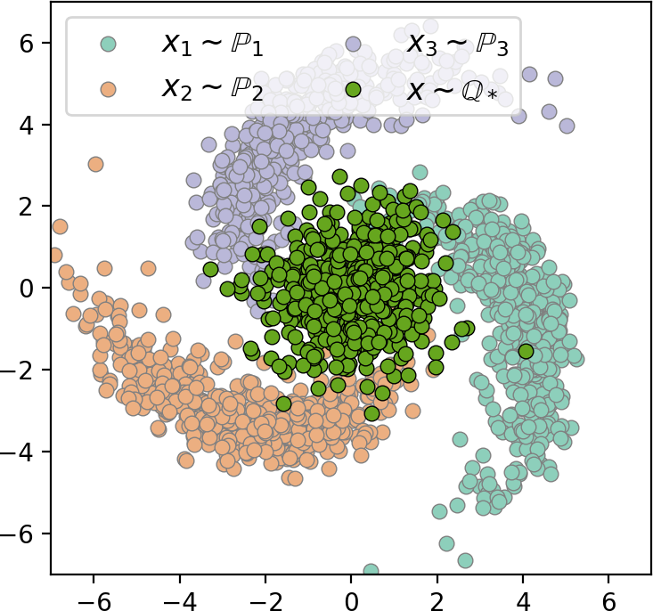
(a) The true unregularized barycenter for the twisted cost.

(b) Our EOT barycenter for the twisted cost (map from $\mathbb{P}_{1}$).

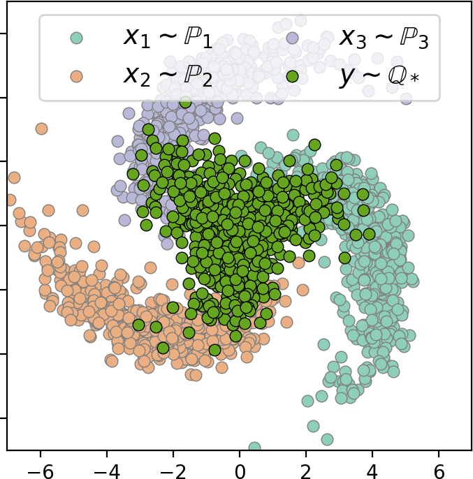
(c) The true unregularized barycenter for $\ell^{2}$ cost.

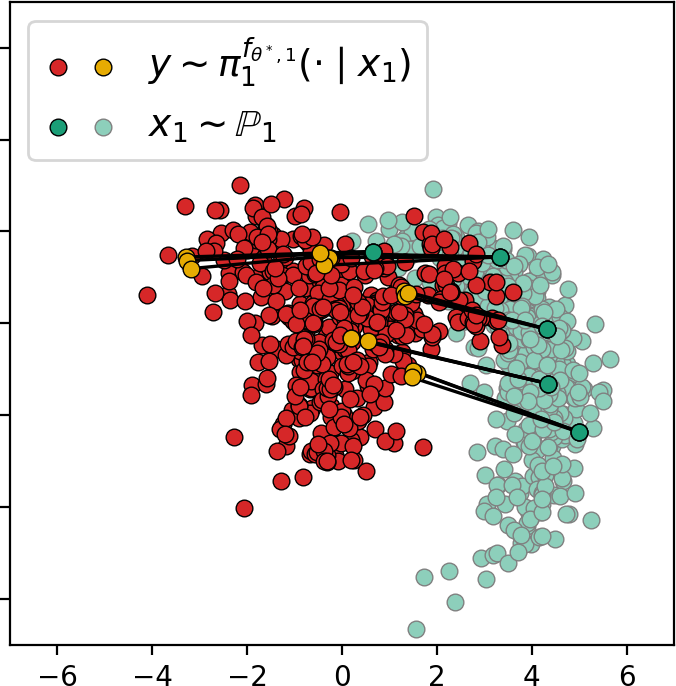
(d) Our EOT barycenter for $\ell^{2}$ cost (map from $\mathbb{P}_{1}$).

Figure 1: 2D twister example: The true barycenter of 3 comets vs. the one computed by our solver with ${\epsilon}=10^{-2}$. Two costs $c_{k}$ are considered: the twisted cost (1(a), 1(b)) and $\ell^{2}$ (1(c), 1(d)).

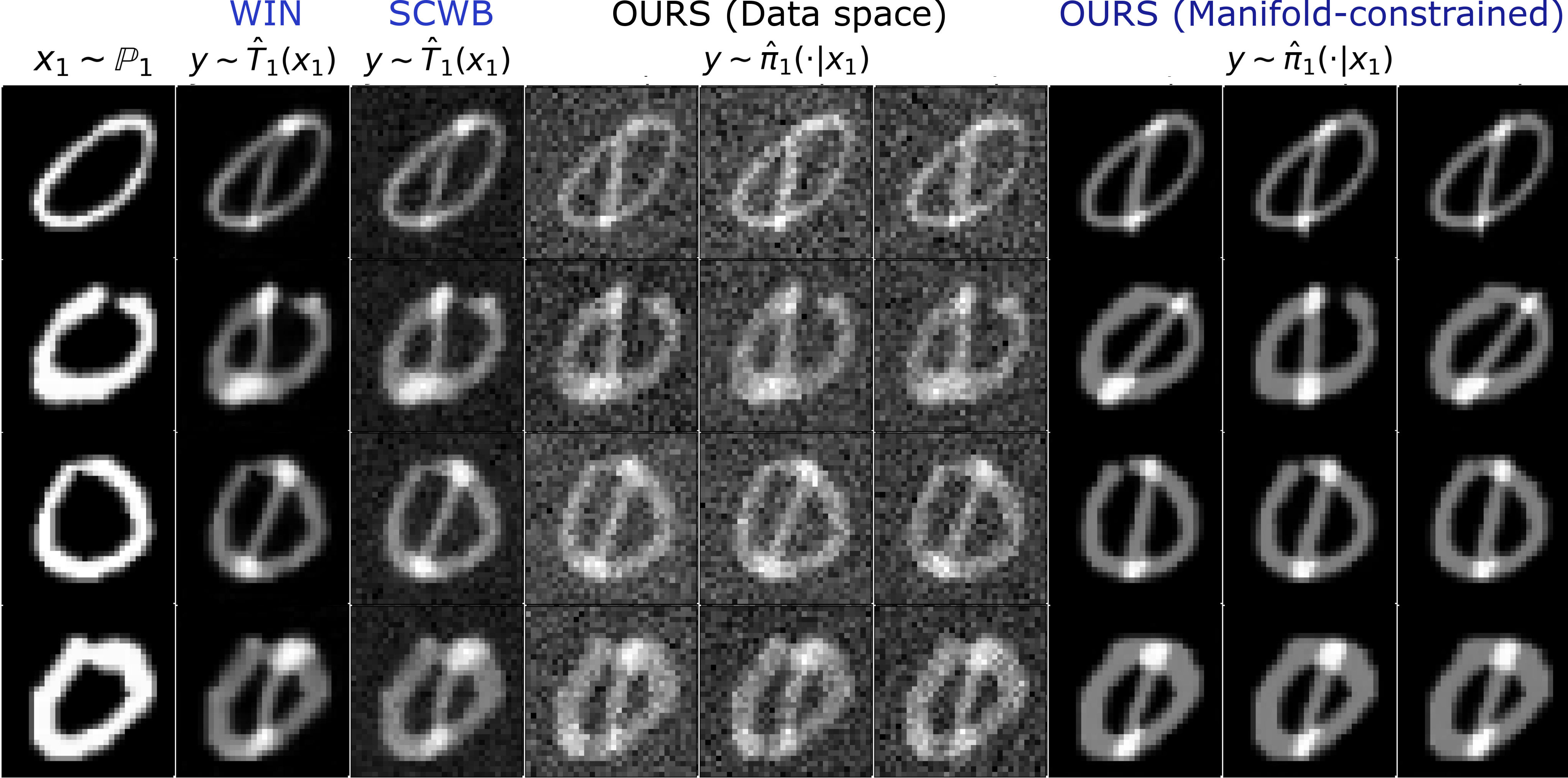
(a) Learned plans from $\mathbb{P}_{1}$ (zeros) to the barycenter.

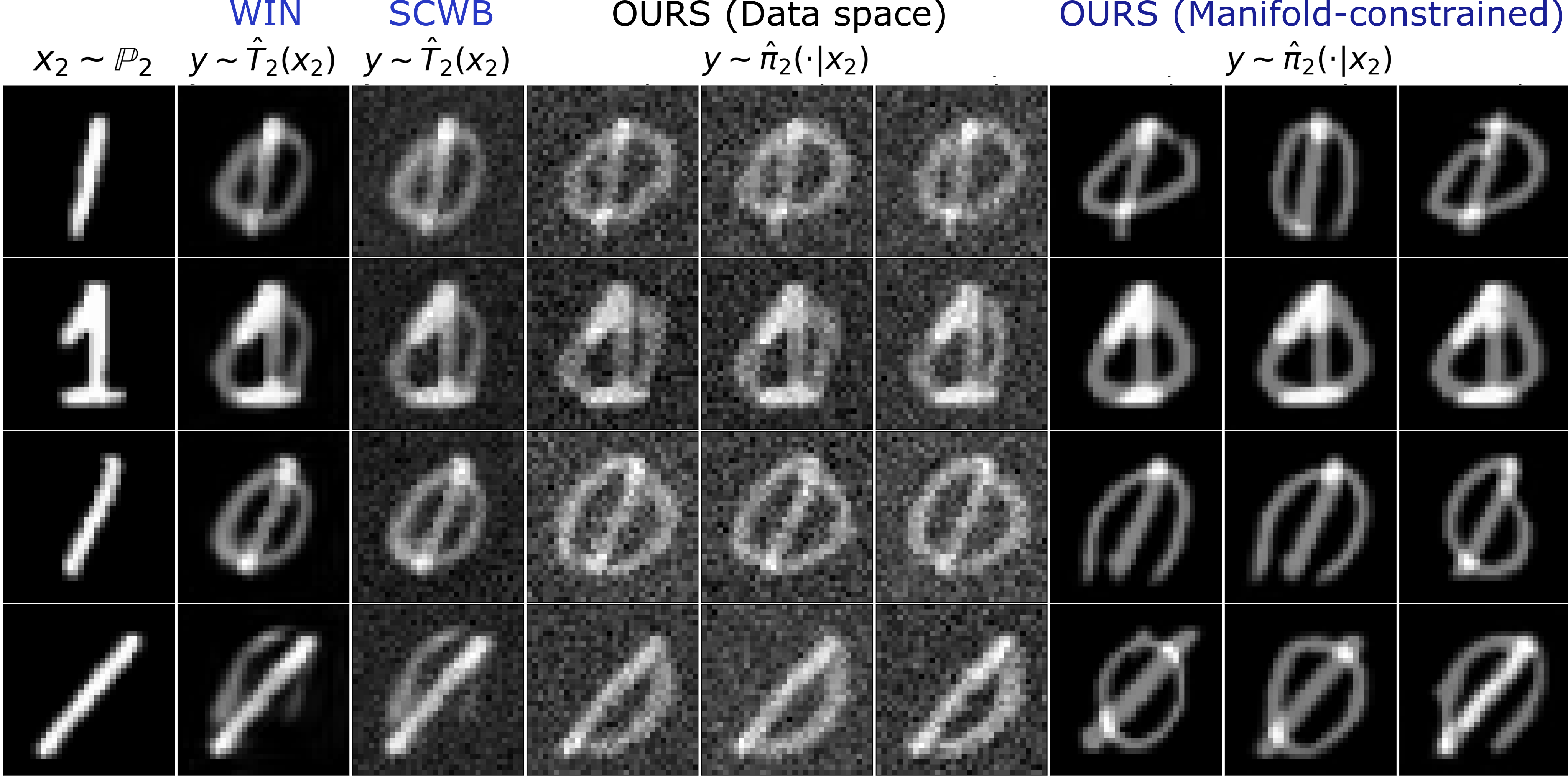
(b) Learned plans from $\mathbb{P}_{2}$ (ones) to the barycenter.

Figure 2: Qualitative comparison of barycenters of MNIST 0/1 digit classes computed with barycenter solvers in the image space w.r.t. the pixel-wise $\ell^{2}$. Solvers SCWB and WIN only learn the unregularized barycenter ($\epsilon=0$) directly in the data space. In turn, our solver learns the EOT barycenter in data space as well as it can learn EOT barycenter restricted to the StyleGAN manifold (${\epsilon}=10^{-2}$).

2D Twister. Consider the map $u:\mathbb{R}^{2}\rightarrow\mathbb{R}^{2}$ which, in the polar coordinate system, is represented by $\mathbb{R}_{+}\times[0,2\pi)\ni(r,\theta)\mapsto\big{(}r,(\theta-r)\text{ mod }2\pi\big{)}$. The cartesian version of $u$ is presented in Appendix C.1. Let $\mathbb{P}_{1},\mathbb{P}_{2},\mathbb{P}_{3}$ be $2$-dimensional distributions as shown in Fig. 1(a). For these distributions and uniform weights $\lambda_{k}=\frac{1}{3}$, the unregularized barycenter ($\epsilon=0$) for the twisted cost $c_{k}(x_{k},y)=\frac{1}{2}\|u(x_{k})-u(y)\|^{2}$ can be derived analytically, see Appendix C.1. The barycenter is the centered Gaussian distribution which is also shown in Fig. 1(a). We run the experiment for this cost with $\epsilon=10^{-2}$, and the results are recorded in Fig. 1(b). We see that it qualitatively coincides with the true barycenter. For completeness, we also show the EOT barycenter computed with our solver for $\ell^{2}(x,y)=\frac{1}{2}\|x-y\|^{2}$ costs (Fig. 1(c)) and the same regularization $\epsilon$. The true $\ell^{2}$ barycenter is estimated by using the free_support_barycenter solver from POT package (Flamary et al., 2021). We stress that the twisted cost barycenter and $\ell^{2}$ barycenter differ, and so do the learned conditional plans: the $\ell^{2}$ EOT plan (Fig. 1(d)) expectedly looks more well-structured while for the twisted cost (Fig. 1(b)) it becomes more chaotic due to non-trivial structure of this cost.

5.2 Barycenters of MNIST Classes 0 and 1

A classic experiment considered in the continuous barycenter literature (Fan et al., 2021; Korotin et al., 2022a; Noble et al., 2023; Cohen et al., 2020) is averaging of distributions of MNIST 0/1 digits with weights $(\frac{1}{2},\frac{1}{2})$ in the grayscale image space $\mathcal{X}_{1}\!=\!\mathcal{X}_{2}\!=\!\mathcal{Y}\!=\![-1,1]^{32\times 32}$. The true unregularized ($\epsilon=0$) $\ell^{2}$-barycenter images $y$ are direct pixel-wise averages $\frac{x_{1}+x_{2}}{2}$ of pairs of images $x_{1}$ and $x_{2}$ coming from the $\ell^{2}$ OT plan between 0’s ($\mathbb{P}_{1}$) and 1’s ($\mathbb{P}_{2}$). In Fig. 2, we show the unregularized $\ell^{2}$ barycenter computed by (Fan et al., 2021, SCWB), (Korotin et al., 2022a, WIN).

Data space EOT barycenter. To begin with, we employ our solver to compute the $\epsilon$-regularized EOT $\ell^{2}$-barycenter directly in the image space $\mathcal{Y}$ for $\epsilon=10^{-2}$. We emphasize that the true entropic barycenter slightly differs from the unregularized one. To be precise, it is expected that regularized barycenter images are close to the unregularized barycenter images but with additional noise. In Fig. 2, we see that our solver (data space) recovers the noisy barycenter images exactly as expected.

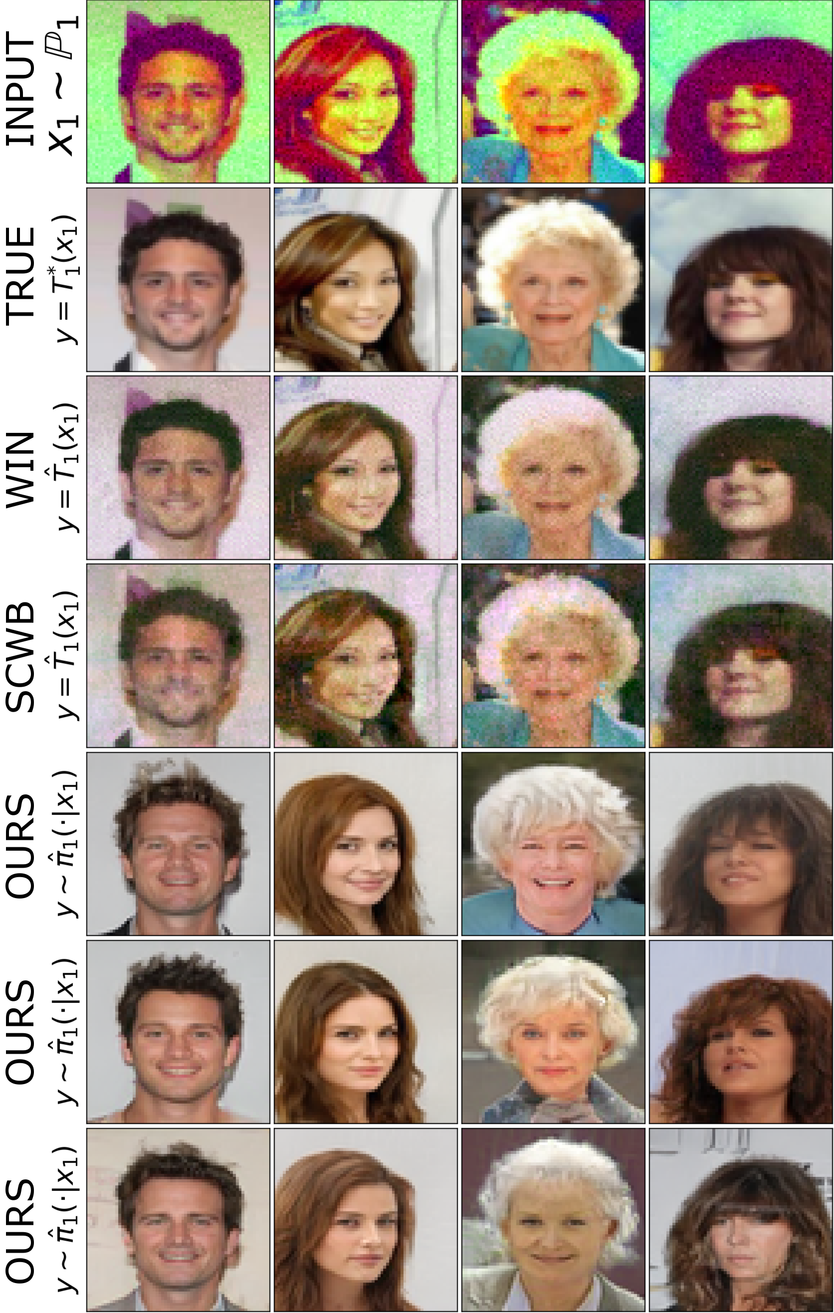
(a) Maps from $\mathbb{P}_{1}$ to the barycenter.

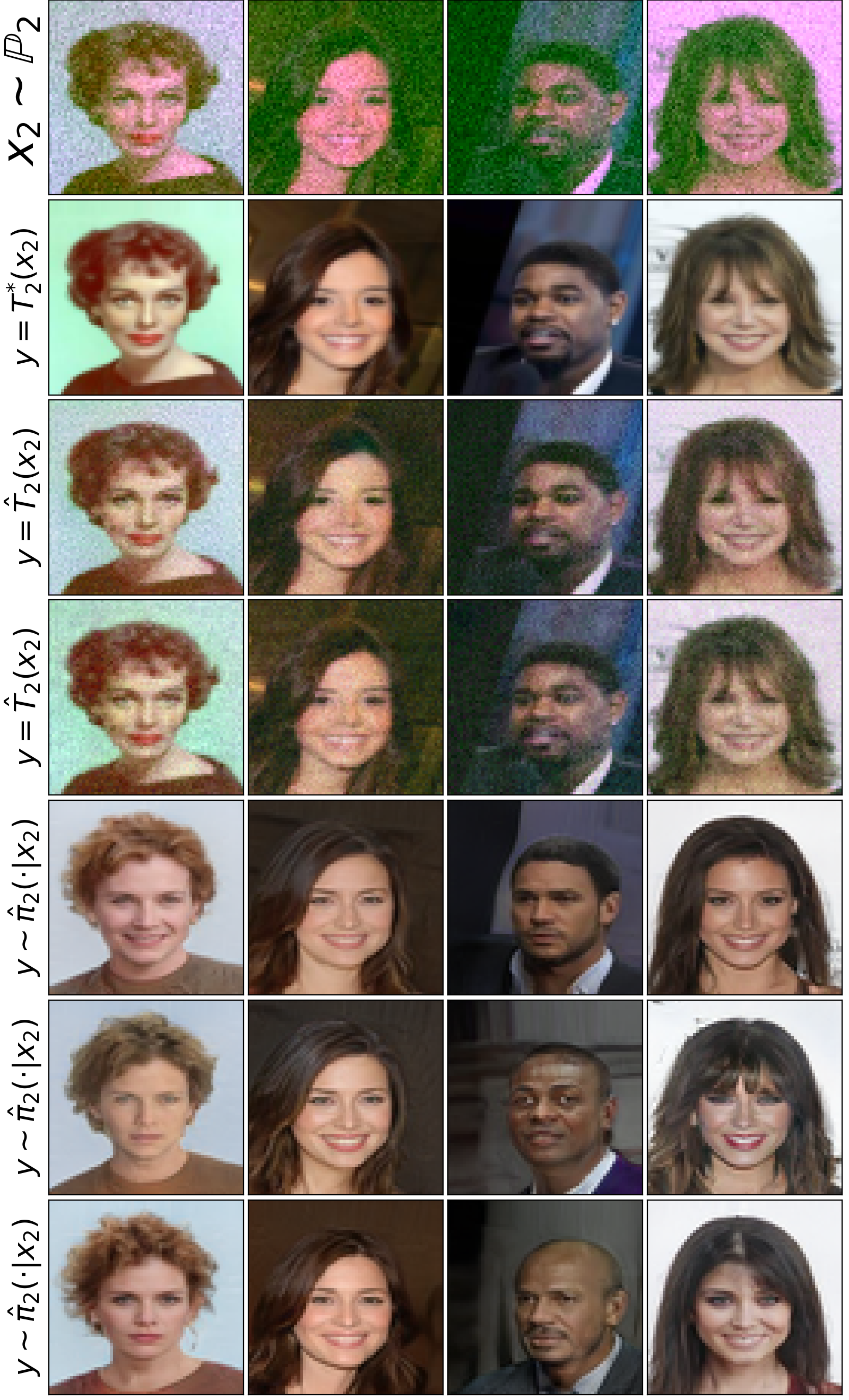
(b) Maps from $\mathbb{P}_{2}$ to the barycenter.

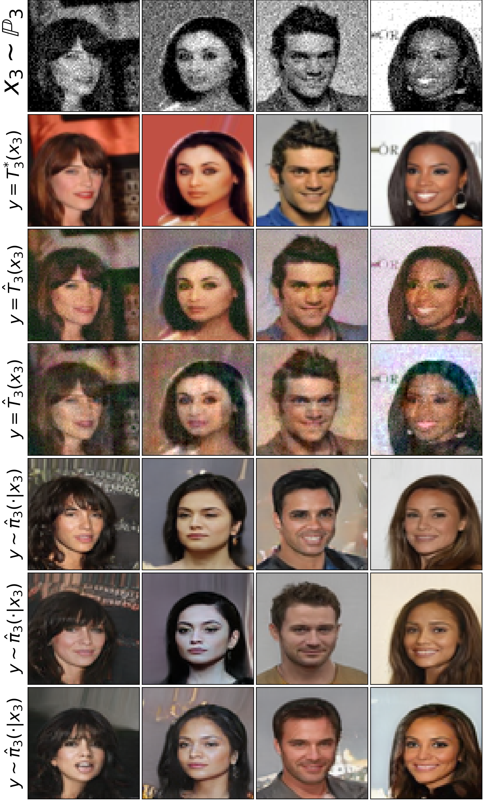
(c) Maps from $\mathbb{P}_{3}$ to the barycenter.

Figure 3: Experiment on the Ave, celeba! barycenter dataset. The plots compare the transported inputs ${x_{k}\sim\mathbb{P}_{k}}$ to the barycenter learned by various solvers. The true unregularized $\ell^{2}$ barycenter of $\mathbb{P}_{1},\mathbb{P}_{2},\mathbb{P}_{3}$ are the clean celebrity faces, see (Korotin et al., 2022a, §5).

Manifold-constrained EOT barycenter. Averaging image distributions directly in the data space can be challenging. Our experiment below shows that if we a priori have some manifold $\mathcal{M}$ where we want the barycenter to be concentrated on, our solver can restrict the search space to it.

As discussed earlier, the support of the image-space unregularized $\ell^{2}$-barycenter is a certain subset of $\mathcal{M}=\{\frac{x_{1}+x_{2}}{2}\text{ }|\text{ }x_{1}\in\text{Supp}(\mathbb{P}_{1}),x_{2}\in\text{Supp}(\mathbb{P}_{1})\}$. To achieve this, we train a StyleGAN model ${G:\mathcal{Z}\rightarrow\mathcal{Y}}$ (Karras et al., 2019) with $\mathcal{Z}=\mathbb{R}^{512}$ to generate an approximate manifold $G(\mathcal{Z})\approx\mathcal{M}$. Then, we use our solver with $\epsilon=10^{-2}$ to search for the barycenter of 0/1 digit distributions on $\mathcal{X}_{1},\mathcal{X}_{2}$ which lies in the latent space $\mathcal{Z}$ w.r.t. costs $c_{k}(x,z)\stackrel{{\scriptstyle\text{def}}}{{=}}\frac{1}{2}\|x-G(z)\|^{2}$ . This can be interpreted as learning the EOT $\ell^{2}$-barycenter in the ambient space but constrained to the StyleGAN-parameterized manifold $G(\mathcal{Z})$. The barycenter $\mathbb{Q}^{*}$ is the distribution of the latent variables $z$, which can be pushed to the manifold $G(\mathcal{Z})\subset\mathcal{Y}$ via $G(z)$. The results are also in Fig. 2. There is no noise compared to the data-space EOT barycenter because of the manifold constraint.

We emphasize that the costs $c_{k}(x_{k},z)$ used here are general (not $\ell^{2}$ cost!) because $G$ is a non-trivial StyleGAN generator. Hence, this experimental setup with the manifold-constrained barycenters is not feasible for most other barycenter solvers as they work exclusively with $\ell^{2}$.

5.3 Evaluation on the Ave, celeba! Dataset

In (Korotin et al., 2022a), the authors developed a theoretically grounded methodology for finding probability distributions whose unregularized $\ell^{2}$ barycenter is known by construction. Based on the CelebA faces dataset (Liu et al., 2015), they constructed an Ave, celeba! dataset containing 3 degraded subsets of faces. The true $\ell^{2}$ barycenter w.r.t. the weights $(\frac{1}{4},\frac{1}{2},\frac{1}{4})$ is the distribution of Celeba faces itself. This dataset is used to test how well our approach recovers the barycenter.

Solver	FID$\downarrow$ of plans to barycenter
	$k\!=\!1$	$k\!=\!2$	$k\!=\!3$
(Fan et al., 2021)	56.7	53.2	58.8
(Korotin et al., 2022a)	49.3	46.9	61.5
Ours	8.4	8.7	10.2

Table 2: FID scores of images mapped
from inputs $\mathbb{P}_{k}$ to the barycenter.

We follow the EOT manifold-constrained setup as in §5.2 and train the StyleGAN on unperturbed celeba faces. This might sound a little bit unfair but our goal is to demonstrate the learned transport plan to the constrained barycenter rather than unconditional barycenter samples (recall the setup in §2.3). Hence, we learn the constrained EOT barycenter with $\epsilon=10^{-4}$. In Fig. 3, we present the results, depicting samples from the learned plans from each $\mathbb{P}_{k}$ to the barycenter. Overall, the map is qualitatively good, although sometimes failures in preserving the image content may occur. This is presumably due to MCMC inference getting stuck in local minima of the energy landscape. For comparison, we also show the results of the solvers by (Fan et al., 2021, SCWB), (Korotin et al., 2022a, WIN). Additionally, we report the FID score (Heusel et al., 2017) for images mapped to the barycenter in Table 2. Owing to the manifold-constrained setup, the FID score of our solver is significantly smaller.

6 Discussion

Potential impact. In our work, we propose a novel approach for solving EOT barycenter problems which is applicable to general OT costs. From the practical viewpoint, we demonstrate the ability to restrict the sought-for barycenter to the image manifold by utilizing a pretrained generative model. Our findings may be applicable to a list of important real-world applications, see Appendix B.2. We believe that our large-scale barycenter solver will leverage industrial & socially-important problems.

Limitations. The limitations of our approach are mostly the same as those of EBMs. It is worth mentioning the usage of MCMC during the training/inference. The basic ULA algorithm which we use in §4.2 may poorly converge to the desired distribution $\mu_{x}^{f}$. In addition, MCMC sampling is time-consuming. We leave the search of more efficient sampling procedures for our solver, e.g., (Levy et al., 2017; Song et al., 2017; Habib & Barber, 2018; Neklyudov et al., 2020; Hoffman et al., 2019; Turitsyn et al., 2011; Lawson et al., 2019; Du et al., 2023), for future research. We also note that our theoretical analysis in §4.3 does not take into the account the optimization errors appearing due to the gradient descent and MCMC. The analysis of these quantities is a completely different domain in machine learning and out of the scope of our work. As the most generative modelling research, we do not attempt to analyse these errors.

7 Broader impact

This paper presents work whose goal is to advance the field of Machine Learning. There are many potential societal consequences of our work, none which we feel must be specifically highlighted here.

8 Acknowledgements

Skoltech was supported by the Analytical center under the RF Government (subsidy agreement 000000D730321P5Q0002, Grant No. 70-2021-00145 02.11.2021). AK acknowledges financial support from the NSERC Discovery Grant No. RGPIN-2023-04482. We would like to express special thanks to Vladimir Vanovskiy from Skoltech for the insightful discussions and details on geological modelling (Appendix B.2).

Appendix A Proofs

A.1 Auxiliary Statements

We start by showing some basic properties of the $C$-transform which will be used in the main proofs.

Proposition A.1 (Properties of the $C$-transform).

Let $f_{1},f_{2}\colon\mathcal{Y}\to\mathbb{R}$ be two measurable functions which are bounded from below. It holds that

1. Monotonicity: $f_{1}\leq f_{2}$ implies $f_{1}^{C}\geq f_{2}^{C}$;

2. Constant additivity: $(f_{1}+a)^{C}=f_{1}^{C}-a$ for all $a\in\mathbb{R}$;

3. Concavity: $(\lambda f_{1}+(1-\lambda)f_{2})^{C}\geq\lambda f_{1}^{C}+(1-\lambda)f_{2}^{C}$ for all $\lambda\in[0,1]$;

4. Continuity: $f_{1},f_{2}$ bounded implies $\sup_{x\in\mathcal{X}}|f_{1}^{C}(x)-f_{2}^{C}(x)|\leq\sup_{y\in\mathcal{Y}}|f_{1}(y)-f_{2}(y)|$.

Proof of Proposition A.1.

We recall the definition of the $C$-transform

$$f_{1}^{C}(x)=\inf_{\mu\in\mathcal{P}(\mathcal{Y})}\left\{C(x,\mu)-\int_{\mathcal{Y}}f_{1}(y)\mathrm{d}\mu(y)\right\},$$

where $C(x,\mu)\stackrel{{\scriptstyle\text{def}}}{{=}}\int_{\mathcal{Y}}c(x,y)\mathrm{d}\mu(y)-\epsilon H(\mu)$. Monotonicity (i) and constant additivity (ii) are immediate from the definition.

To see (iii), observe that the dependence of $\int_{\mathcal{Y}}f_{1}(y)\mathrm{d}\mu(y)$ on $f_{1}$ is linear. Thus, $f_{1}^{C}$ is the pointwise infimum of a family of linear functionals and thus concave.

Finally, to show (iv) we have by monotonicity of the integral that

$$\left|\int_{\mathcal{Y}}f_{1}(y)\mathrm{d}\mu(y)-\int_{\mathcal{Y}}f_{2}(y)\mathrm{d}\mu(y)\right|\leq\sup_{y\in\mathcal{Y}}|f_{1}(y)-f_{2}(y)|$$ (22)

for any $\mu\in\mathcal{P}(\mathcal{Y})$. For fixed $x\in\mathcal{X}$ we have

$$f_{1}^{C}(x)-f_{2}^{C}(x) =\inf_{\mu\in\mathcal{P}(\mathcal{Y})}\left[C(x,\tilde{\mu})-\int_{\mathcal{Y}}f_{1}(y)\mathrm{d}\tilde{\mu}(y)\right]-\inf_{\mu\in\mathcal{P}(\mathcal{Y})}\left[C(x,\mu)-\int_{\mathcal{Y}}f_{2}(y)\mathrm{d}\mu(y)\right]$$

$$=\sup_{\mu\in\mathcal{P}(\mathcal{Y})}\inf_{\tilde{\mu}\in\mathcal{P}(\mathcal{Y})}\left[C(x,\tilde{\mu})-C(x,\mu)-\int_{\mathcal{Y}}f_{1}(y)\mathrm{d}\tilde{\mu}(y)+\int_{\mathcal{Y}}f_{2}(y)\mathrm{d}\mu(y)\right].$$

By setting $\tilde{\mu}=\mu$ we increase the value and obtain

$$f_{1}^{C}(x)-f_{2}^{C}(x)\leq\sup_{\mu\in\mathcal{P}(\mathcal{Y})}\int_{\mathcal{Y}}\left[f_{2}(y)-f_{1}(y)\right]\mathrm{d}\mu(y)\leq\sup_{y\in\mathcal{Y}}|f_{1}(y)-f_{2}(y)|,$$ (23)

where the last inequality follows from (22). For symmetry reasons, we can swap the roles of $f_{1}$ and $f_{2}$ in (23), which yields the claim. ∎

A.2 Proof of Theorem 4.1

Proof.

By substituting in (8) the primal EOT problems (2) with their dual counterparts (3), we obtain a dual formulation, which is the starting point of our analysis:

$$\mathcal{L}^{*}=\min\limits_{\mathbb{Q}\in\mathcal{P}(\mathcal{Y})}\sup\limits_{f_{1},\dots,f_{K}\in\mathcal{C}(\mathcal{Y})}\underbrace{\sum\limits_{k=1}^{K}\lambda_{k}\bigg{\{}\int_{\mathcal{X}_{k}}f^{C_{k}}_{k}(x_{k})\mathrm{d}\mathbb{P}_{k}(x_{k})+\int_{\mathcal{Y}}f_{k}(y)\mathrm{d}\mathbb{Q}(y)\bigg{\}}}_{\stackrel{{\scriptstyle\text{def}}}{{=}}\widetilde{\mathcal{L}}\big{(}\mathbb{Q},\{f_{k}\}_{k=1}^{K}\big{)}}.$$ (24)

Here, we replaced $\inf$ with $\min$ because of the existence of the barycenter (§2.2). Moreover, we refer to the entire expression under the $\min\sup$ as a functional $\widetilde{\mathcal{L}}\colon\mathcal{P}(\mathcal{Y})\times\mathcal{C}(\mathcal{Y})^{K}\rightarrow\mathbb{R}$. For brevity, we introduce, for $(f_{1},\ldots,f_{K})\in\mathcal{C}(\mathcal{Y})^{K}$, the notation

$$\bar{f}\stackrel{{\scriptstyle\text{def}}}{{=}}\sum_{k=1}^{K}\lambda_{k}f_{k}\quad\text{and}\quad M\stackrel{{\scriptstyle\text{def}}}{{=}}\inf_{y\in\mathcal{Y}}\bar{f}(y)=\inf_{\mathbb{Q}\in\mathcal{P}(\mathcal{Y})}\int\bar{f}(y)\mathrm{d}\mathbb{Q}(y),$$ (25)

where the equality follows from two elementary observations that (a) $M\leq\int\bar{f}(y)\mathrm{d}\mathbb{Q}(y)$ for any $\mathbb{Q}\in\mathcal{P}(\mathcal{Y})$ and (b) $\bar{f}(y)=\int\bar{f}(y^{\prime})\mathrm{d}\delta_{y}(y^{\prime})$ where $\delta_{y}$ denotes a Dirac mass at $y\in\mathcal{Y}$.

On the one hand, $\mathcal{P}(\mathcal{Y})$ is compact w.r.t. the weak topology because $\mathcal{Y}$ is compact, and for fixed potentials $(f_{1},\ldots,f_{K})\in\mathcal{P}(\mathcal{Y})^{K}$ we have that $\widetilde{\mathcal{L}}(\cdot,(f_{k})_{k=1}^{K})$ is continuous and linear. In particular, $\widetilde{\mathcal{L}}(\cdot,(f_{k})_{k=1}^{K})$ is convex and l.s.c. On the other hand, for a fixed $\mathbb{Q}$, the functional $\widetilde{\mathcal{L}}\big{(}\mathbb{Q},\cdot\big{)}$ is concave by (iii) in Proposition A.1. These observations allow us to apply Sion’s minimax theorem (Sion, 1958, Theorem 3.4) to swap $\min$ and $\inf$ in (24) and obtain using (25)

$$\mathcal{L}^{*} =\sup_{f_{1},\dots,f_{K}\in\mathcal{C}(\mathcal{Y})}\min_{\mathbb{Q}\in\mathcal{P}(\mathcal{Y})}\sum_{k=1}^{K}\lambda_{k}\bigg{\{}\int_{\mathcal{X}_{k}}f^{C_{k}}_{k}(x_{k})\mathrm{d}\mathbb{P}_{k}(x_{k})+\int_{\mathcal{X}}f_{k}(y)\mathrm{d}\mathbb{Q}(y)\bigg{\}}$$

$$=\sup_{f_{1},\dots,f_{K}\in\mathcal{C}(\mathcal{Y})}\bigg{\{}\sum_{k=1}^{K}\lambda_{k}\int_{\mathcal{X}_{k}}f^{C_{k}}_{k}(x_{k})\mathrm{d}\mathbb{P}_{k}(x_{k})+\min\limits_{\mathbb{Q}\in\mathcal{P}(\mathcal{Y})}\int_{\mathcal{X}}\bar{f}(y)\mathrm{d}\mathbb{Q}(y)\bigg{\}}$$

$$=\sup\limits_{f_{1},\dots,f_{K}\in\mathcal{C}(\mathcal{Y})}\underbrace{\bigg{\{}\sum\limits_{k=1}^{K}\lambda_{k}\int_{\mathcal{X}_{k}}f^{C_{k}}_{k}(x_{k})\mathrm{d}\mathbb{P}_{k}(x_{k})+\min_{y\in\mathcal{Y}}\bar{f}(y)\bigg{\}}}_{\stackrel{{\scriptstyle\text{def}}}{{=}}\widetilde{\mathcal{L}}(f_{1},\dots,f_{K})}.$$ (26)

Next, we show that the $\sup$ in (26) can be restricted to tuplets satisfying the congruence condition $\sum_{k=1}^{K}\lambda_{k}f_{k}=0$. It remains to show that for every tuplet $(f_{1},\dots,f_{K})\in\mathcal{C}(\mathcal{Y})^{K}$ there exists a congruent tuplet $(\tilde{f}_{1},\dots,\tilde{f}_{K})\in\mathcal{C}(\mathcal{Y})^{K}$ such that $\widetilde{\mathcal{L}}(\tilde{f}_{1},\dots,\tilde{f}_{K})\geq\widetilde{\mathcal{L}}(f_{1},\dots,f_{K})$.

To this end, fix $(f_{1},\dots,f_{K})$ and define the congruent tuplet

$$(\tilde{f}_{1},\dots,\tilde{f}_{K})\stackrel{{\scriptstyle\text{def}}}{{=}}\left(f_{1},\dots,f_{K-1},f_{K}-\frac{\bar{f}}{\lambda_{K}}\right).$$ (27)

We find $\tilde{M}\stackrel{{\scriptstyle\text{def}}}{{=}}\inf_{y\in\mathcal{Y}}\sum_{k=1}^{K}\lambda_{k}\tilde{f}_{k}=0$ by the congruence and derive

$$\widetilde{\mathcal{L}}(\tilde{f}_{1},\dots,\tilde{f}_{K})-\widetilde{\mathcal{L}}(f_{1},\dots,f_{K}) =\lambda_{K}\int_{\mathcal{X}_{K}}\left[\tilde{f}_{K}^{C_{K}}(x_{K})-f^{C_{K}}_{K}(x_{K})\right]\mathrm{d}\mathbb{P}_{K}(x_{K})-M$$

$$\geq\lambda_{K}\int_{\mathcal{X}_{K}}\left[\left(f_{K}-\frac{M}{\lambda_{K}}\right)^{C_{K}}(x_{K})-f_{K}^{C_{K}}(x_{K})\right]\mathrm{d}\mathbb{P}(x_{K})-M$$

$$=\lambda_{K}\int_{\mathcal{X}_{K}}\frac{M}{\lambda_{K}}\mathrm{d}\mathbb{P}(x_{K})-M=0,$$

where the first inequality follows from $\tilde{f}_{K}=f_{K}-\frac{\bar{f}}{\lambda_{K}}\leq f_{K}-\frac{M}{\lambda_{K}}$ combined with monotonicity of the $C$-transform, see (i) in Proposition A.1. The second to last equality follow from constant additivity, see (ii) in Proposition A.1.

In summary, we obtain

$$\mathcal{L}^{\ast}=\sup_{\begin{subarray}{c}f_{1},\ldots,f_{k}\in\mathcal{C}(\mathcal{Y})\\ \sum_{k=1}^{K}f_{k}=0\end{subarray}}\widetilde{\mathcal{L}}(f_{1},\ldots,f_{K}).$$ (28)

Finally, observe that for congruent $(f_{1},\ldots,f_{K})$ we have $\widetilde{\mathcal{L}}(f_{1},\ldots,f_{K})=\mathcal{L}(f_{1},\ldots,f_{K})$. Hence, we can replace $\widetilde{\mathcal{L}}$ by $\mathcal{L}$ in (28), which yields (LABEL:EOT_bary_dual_our). ∎

A.3 Proof of Theorem 4.2

Proof.

Write $\mathbb{Q}^{\ast}$ for the barycenter and $\pi^{\ast}_{k}$ for the optimizer of $\text{EOT}_{c_{k},\epsilon}(\mathbb{P}_{k},\mathbb{Q}^{\ast})$. Consider congruent potentials $f_{1},\ldots,f_{K}\in\mathcal{C}(\mathcal{Y})$ and define the probability distribution

$$\mathrm{d}\pi^{f_{k}}(x_{k},y)\stackrel{{\scriptstyle\text{def}}}{{=}}\mathrm{d}\mu_{x_{k}}^{f_{k}}(y)\,\mathrm{d}\mathbb{P}_{k}(x_{k}),$$

where

$$\frac{\mathrm{d}\mu^{f_{k}}_{x_{k}}(y)}{\mathrm{d}y} \stackrel{{\scriptstyle\text{def}}}{{=}}\frac{1}{Z_{c_{k}}(f_{k},x_{k})}\exp\left(\frac{f_{k}(y)-c_{k}(x_{k},y)}{\epsilon}\right),$$ (29)

$$Z_{c_{k}}(f_{k},x_{k}) \stackrel{{\scriptstyle\text{def}}}{{=}}\log\left(\int_{\mathcal{Y}}e^{\frac{f_{k}(y)-c_{k}(x_{k},y)}{\epsilon}}\mathrm{d}y\right).$$ (30)

Then we have by (6)

$$\text{EOT}_{c_{k},\epsilon}(\mathbb{P}_{k},\mathbb{Q}^{\ast})-\left(\int_{\mathcal{X}_{k}}f^{C_{k}}(x_{k})\mathrm{d}\mathbb{P}(x_{k})+\int_{\mathcal{Y}}f(y)\mathrm{d}\mathbb{Q}^{*}(y)\right)=\epsilon\text{KL}\left(\pi_{k}^{*}\|\pi^{f_{k}}\right).$$ (31)

Multiplying (31) by $\lambda_{k}$ and summing over $k$ yields

$$\epsilon\sum_{k=1}^{K}\lambda_{k}\text{KL}\left(\pi_{k}^{*}\|\pi^{f_{k}}\right) =\sum_{k=1}\lambda_{k}\left\{\text{EOT}_{c_{k},\epsilon}(\mathbb{P}_{k},\mathbb{Q}^{\ast})-\int_{\mathcal{X}_{k}}f^{C_{k}}_{k}(x_{k})\mathrm{d}\mathbb{P}_{k}(x_{k})\right\}-\int_{\mathcal{Y}}\underbrace{\sum_{k=1}^{K}\lambda_{k}f(y)}_{=0}\mathrm{d}\mathbb{Q}^{\ast}(y)$$

$$=\mathcal{L}^{\ast}-\mathcal{L}(f_{1},\ldots,f_{k}),$$ (32)

where the last equality follows by congruence, i.e., $\sum_{k=1}^{K}\lambda_{k}f_{k}\equiv 0$.

The remaining inequality in (12) is a consequence of the data processing inequality for $f$-divergences which we invoke here to get

$$\text{KL}\left(\pi_{k}^{\ast}\|\pi^{f_{k}}\right)\geq\text{KL}\left(\mathbb{Q}^{\ast}\|\mathbb{Q}^{f_{k}}\right),$$

where $\mathbb{Q}^{\ast}$ and $\mathbb{Q}^{f_{k}}$ are the second marginals of $\pi^{\ast}_{k}$ and $\pi^{f_{k}}$, respectively. ∎

A.4 Proof of Theorem 4.3

Proof.

The desired equation (LABEL:weak_EOT_bary_loss_grad) could be derived exactly the same way as in (Mokrov et al., 2024, Theorem 3). ∎

A.5 Proof of Proposition 4.4 and Theorem 4.5

The derivations of the quantitative bound for Proposition 4.4 and Theorem 4.5 relies on the following standard definitions from learning theory, which we now recall for convenience (see, e.g. (Shalev-Shwartz & Ben-David, 2014, §26)). Consider some class $\mathcal{S}$ of functions $s:\mathcal{X}\rightarrow\mathbb{R}$ and a distribution $\mu$ on $\mathcal{X}$. Let $X=\{x^{1},\dots,x^{N}\}$ be a sample of $N$ points in $\mathcal{X}$.

The representativeness of the sample $X$ w.r.t. the class $\mathcal{S}$ and the distribution $\mu$ is defined by

$$\text{Rep}_{X}(\mathcal{S},\mu)\stackrel{{\scriptstyle\text{def}}}{{=}}\sup_{s\in\mathcal{S}}\big{[}\int_{\mathcal{X}}s(x)\mathrm{d}\mu(x)-\frac{1}{N}\sum_{n=1}^{N}s(x^{n})\big{]}.$$ (33)

The Rademacher complexity of the class $\mathcal{S}$ w.r.t. the distribution $\mu$ and sample size $N$ is given by

$$\mathcal{R}_{N}(\mathcal{S},\mu)\stackrel{{\scriptstyle\text{def}}}{{=}}\frac{1}{N}\mathbb{E}\bigg{\{}\sup_{s\in\mathcal{S}}\sum_{n=1}^{N}s(x^{n})\sigma_{n}\bigg{\}},$$ (34)

where $\{x^{n}\}_{n=1}^{N}\sim\mu$ are mutually independent, $\{\sigma^{n}\}_{n=1}^{N}$ are mutually independent Rademacher random variables, i.e., $\text{Prob}\big{(}\sigma^{n}=1\big{)}=\text{Prob}\big{(}\sigma^{n}=-1\big{)}=0.5$, and the expectation is taken with respect to both $\{x_{n}\}_{n=1}^{N}$, $\{\sigma_{n}\}_{n=1}^{N}$. The well-celebrated relation between (34) and $\eqref{representativeness-def}$, as shown in (Shalev-Shwartz & Ben-David, 2014, Lemma 26.2), is

$$\mathbb{E}\text{Rep}_{X}(\mathcal{S},\mu)\leq 2\cdot\mathcal{R}_{N}(\mathcal{S},\mu),$$ (35)

where the expectation is taken w.r.t. random i.i.d. sample $X\sim\mu$ of size $N$.

Proposition 4.4.

Observe that by (32) we may write

$$\epsilon\sum_{k=1}^{K}\lambda_{k}\text{KL}\left(\pi_{k}^{*}\|\pi^{\widehat{f}_{k}}\right)=\mathcal{L}^{*}-\mathcal{L}(\widehat{\textbf{f}})=\underbrace{\bigg{[}\mathcal{L}^{*}-\max\limits_{\scriptsize\textbf{f}\in\overline{\mathcal{F}}}\mathcal{L}(\textbf{f})\bigg{]}}_{\text{Approximation error}}+\underbrace{\bigg{[}\max\limits_{\scriptsize\textbf{f}\in\overline{\mathcal{F}}}\mathcal{L}(\textbf{f})-\mathcal{L}(\widehat{\textbf{f}})\bigg{]}}_{\text{Estimation error}}.$$ (36)

Let $\overline{\textbf{f}}$ be a maximizer of $\mathcal{L}(\textbf{f})$ within $\overline{\mathcal{F}}$. Analysing the estimation error in (36) yields

$$\max\limits_{\scriptsize\textbf{f}\in\overline{\mathcal{F}}}\mathcal{L}(\textbf{f})-\mathcal{L}(\widehat{\textbf{f}}) =\mathcal{L}(\overline{\textbf{f}})-\mathcal{L}(\widehat{\textbf{f}})$$

$$=\big{[}\mathcal{L}(\overline{\textbf{f}})-\widehat{\mathcal{L}}(\overline{\textbf{f}})\big{]}+\underbrace{\big{[}\widehat{\mathcal{L}}(\overline{\textbf{f}})-\widehat{\mathcal{L}}(\widehat{\textbf{f}})\big{]}}_{\leq 0}+\big{[}\widehat{\mathcal{L}}(\widehat{\textbf{f}})-\mathcal{L}(\widehat{\textbf{f}})\big{]}$$ (37)

$$\leq\,2\sup_{\textbf{f}\in\overline{\mathcal{F}}}\big{|}\mathcal{L}(\textbf{f})-\widehat{\mathcal{L}}(\textbf{f})\big{|},$$ (38)

where central term in line (37) is bounded above by $0$ due the maximality of $\widehat{\textbf{f}}$, that is, $\widehat{\mathcal{L}}(\widehat{\textbf{f}})=\max_{\textbf{f}\in\overline{\mathcal{F}}}\widehat{\mathcal{L}}(\textbf{f})\geq\widehat{\mathcal{L}}(\overline{\textbf{f}})$. Due to (38), we can bound the estimation error using the Rademacher complexity

$$\sup_{\textbf{f}\in\overline{\mathcal{F}}}\big{|}\mathcal{L}(\textbf{f})-\widehat{\mathcal{L}}(\textbf{f})\big{|}\leq\sum_{k=1}^{K}\lambda_{k}\sup_{f_{k}\in\mathcal{F}_{k}}\biggl{[}\int_{\mathcal{X}_{k}}f^{C_{k}}_{k}(x_{k})\mathrm{d}\mathbb{P}_{k}(x_{k})-\frac{1}{N_{k}}\sum_{n=1}^{N_{k}}f_{k}^{C_{k}}(x_{k}^{n})\biggr{]}=\sum_{k=1}^{K}\lambda_{k}\text{Rep}_{X_{k}}(\mathcal{F}_{k}^{C_{k}},\mathbb{P}_{k}).$$

∎

Proof of Theorem 4.5.

Case (a) - Lipschitz costs: Assume that, for $k\in\overline{K}$, $x\mapsto c_{k}(x,y)$ is Lipschitz with constant $L_{k}\geq 0$ for every $y\in\mathcal{Y}$. Recall that $f^{C_{k}}_{k}$ is defined as the pointwise supremum of $L_{k}$-Lipschitz functions and, therefore, Lipschitz continuous with the same constant. Since the value of the representativeness of a sample w.r.t. a function class is invariant under translating individual elements of said class, we have that $\text{Rep}_{X}(\mathcal{F}_{k}^{C_{k}},\mathbb{P}_{k})$ coincides with $\text{Rep}_{X}(\mathcal{G}_{k},\mathbb{P}_{k})$ where

$$\mathcal{G}_{k}\stackrel{{\scriptstyle\text{def}}}{{=}}\{f^{C_{k}}-f^{C_{k}}(\tilde{x}_{k}):f\in C(\mathcal{Y})\},$$

for some fixed $\tilde{x}_{k}\in\mathcal{X}_{k}$. All the functions in this class are $L_{k}$-Lipschitz and, therefore, bounded by $L_{k}\cdot\text{diam}(\mathcal{X}_{k})$. We may therefore apply (Gottlieb et al., 2016, Theorem 4.3) to the class $\mathcal{G}_{k}$ and obtain

$$\mathbb{E}_{X\sim\mathbb{P}_{k}}\text{Rep}_{X}(\mathcal{F}^{C_{k}}_{k},\mathbb{P}_{k})=\mathbb{E}_{X\sim\mathbb{P}_{k}}\text{Rep}_{X}(\mathcal{G}_{k},\mathbb{P}_{k})\leq 2\mathcal{R}_{N}(\mathcal{G}_{k},\mathbb{P}_{k})\leq O(N_{k}^{-\frac{1}{D_{k}+1}}).$$

Case (b) - Feature-based quadratic costs $\frac{1}{2}\|u_{k}(\cdot)-v(\cdot)\|_{2}^{2}$: Alternatively, consider the case where $c_{k}(x_{k},y)=\frac{1}{2}\|u_{k}(x_{k})-v(y)\|_{2}^{2}$ and $\mathcal{F}_{k}\subseteq\mathcal{C}(\mathcal{Y})$ is bounded (w.r.t. the supremum norm).

To this end, recall that for a measurable and bounded function $f:\mathcal{Y}\to\mathbb{R}$, the weak entropic $c_{k}$-transform satisfies

$$f^{C_{k}}(x_{k})=-\epsilon\log(Z_{c_{k}}(f,x_{k})),$$

where $Z_{c_{k}}(f,x_{k})=\int_{\mathcal{Y}}\exp\big{(}\frac{f(y)-c_{k}(x_{k},y)}{\epsilon}\big{)}\,dy$. Recall that $\mathbb{R}^{D^{\prime\prime}}\times\mathbb{R}^{D^{\prime\prime}}\ni(a,b)\mapsto\exp(-\frac{\|a-b\|^{2}}{2\epsilon})$ is a positive definite kernel which is widely known as the Gaussian kernel. This means that there exists a Hilbert space $\mathcal{H}$ and a feature map $\phi:\mathbb{R}^{D^{\prime\prime}}\to\mathcal{H}$ such that $\exp(-\frac{\|a-b\|^{2}}{2\epsilon})=\langle\phi(a),\phi(b)\rangle_{\mathcal{H}}.$ Due to the particular form of $c_{k}$, we may write

$$\exp\Big{(}-\frac{c_{k}(x_{k},y)}{\epsilon}\Big{)}=\exp\Big{(}-\frac{\|u_{k}(x)-v(y)\|^{2}}{2\epsilon}\Big{)}=\langle\phi(u_{k}(x_{k})),\phi(v(y))\rangle_{\mathcal{H}}.$$ (39)

Notice that $\{\phi(u_{k}(x_{k})):x_{k}\in\mathcal{X}_{k}\}\subseteq\{v\in\mathcal{H}:\,\|v\|_{\mathcal{H}}=1\}$ since $\|\phi(a)\|_{\mathcal{H}}^{2}=\langle\phi(a),\phi(a)\rangle_{\mathcal{H}}=1$ for every $a\in\mathbb{R}^{D^{\prime\prime}}$.

Using the identity in (39), we can express $Z_{c_{k}}(f,x_{k})$ by

$$Z_{c_{k}}(f,x_{k})=\int_{\mathcal{Y}}\langle\phi(u_{k}(x_{k})),\phi(v(y))\rangle_{\mathcal{H}}\,e^{\frac{f(y)}{\epsilon}}\,dy=\Big{\langle}\phi\big{(}u_{k}(x_{k})\big{)},\int_{\mathcal{Y}}\phi(v(y))e^{\frac{f(y)}{\epsilon}}\,dy\Big{\rangle}_{\mathcal{H}},$$

where the last equality is justified as $\mathcal{Y}$ is compact; furthermore, we note the integrals are well-defined by the measurability of $\phi$, $u_{k}$ and $v$. Moreover, using the boundedness of each $\mathcal{F}_{k}$ and compactness of $\mathcal{Y}$, we get

$$R\stackrel{{\scriptstyle\text{def}}}{{=}}\max_{k=1,\ldots,K}\sup_{f\in\mathcal{F}_{k}}\Big{\|}\int_{\mathcal{Y}}\phi(v(y))e^{\frac{f(y)}{\epsilon}}\,dy\Big{\|}_{\mathcal{H}}<\infty.$$ (40)

Define $\mathcal{G}_{k}\stackrel{{\scriptstyle\text{def}}}{{=}}\{Z_{c_{k}}(f,\cdot):f\in\mathcal{F}_{k}\}$ and observe that $\mathcal{G}_{k}\subseteq\mathcal{G}_{k}^{\prime}\stackrel{{\scriptstyle\text{def}}}{{=}}\{\langle\phi\big{(}u_{k}(\cdot)\big{)},w\rangle_{\mathcal{H}}:\|w\|_{\mathcal{H}}\leq R\}.$ This implies that $\mathcal{R}_{N_{k}}(\mathcal{G}_{k},\mathbb{P}_{k})\leq\mathcal{R}_{N_{k}}(\mathcal{G}_{k}^{\prime},\mathbb{P}_{k})$ by the properties of the Rademacher complexity. In turn, the latter Rademacher complexity can be bounded by (Bartlett & Mendelson, 2002, Lemma 22). Indeed, write $\mathbb{P}_{k}^{\prime}\stackrel{{\scriptstyle\text{def}}}{{=}}(u_{k})_{\#}\mathbb{P}_{k}$ such that

$$\mathcal{R}_{N_{k}}(\mathcal{G}_{k}^{\prime},\mathbb{P}_{k})=\mathcal{R}_{N_{k}}(\{\langle\phi(\cdot),w\rangle_{\mathcal{H}}:\|w\|_{\mathcal{H}}\leq R\},\mathbb{P}_{k}^{\prime}),$$

which can be directly seen from the definition of the Rademacher complexity. Thus, we can apply (Bartlett & Mendelson, 2002, Lemma 22) to the right-hand side, and summarizing obtain

$$\mathcal{R}_{N_{k}}(\mathcal{G}_{k},\mathbb{P}_{k})\leq\frac{R}{\sqrt{N_{k}}}.$$

Since the functions in $\mathcal{G}_{k}$ are bounded uniformly away from zero by some constant $\kappa>0$ (depending on the bound of $\mathcal{F}_{k}$ and $\epsilon$), and since the logarithm restricted to $[\kappa,\infty)$ is $1/\kappa$-Lipschitz, we have that

$$\mathcal{R}_{N_{k}}(\mathcal{F}_{k}^{C_{k}},\mathbb{P}_{k})\leq\frac{\epsilon}{\kappa}\mathcal{R}_{N_{k}}(\mathcal{G}_{k},\mathbb{P}_{k})\leq\frac{\epsilon}{\kappa}\,\frac{R}{\sqrt{N_{k}}}.$$

We can now bound the expected representativeness of $\mathcal{F}_{k}^{C_{k}}$ with the Rademacher complexity by (35), yielding the claim. ∎

A.6 Proof of Theorem 4.6

Proof of Theorem 4.6.

Let $\sigma\in C(\mathbb{R})$ be a non-affine activation function which is differentiable at some point $x_{0}\in\mathbb{R}$ and for which $\sigma^{\prime}(x_{0})\neq 0$. Let $\delta>0$, $\lambda_{1},\dots,\lambda_{K}>0$, and $K\in\mathbb{N}$ be given. By Theorem 4.1, there exist $K$ congruent continuous functions $f_{1}^{\prime},\dots,f_{K}^{\prime}$ such that

$$\mathcal{L}^{*}-\mathcal{L}(\tilde{f_{1}},\dots,\tilde{f_{K}})<\frac{\delta}{2}.$$ (41)

Applying (Dugundji, 1951, Theorem 4.1) we deduce that for each $k=1,\dots,K$, there exist a continuous extension $f_{k}^{\prime}:\mathbb{R}^{D}\to\mathbb{R}$ for $\tilde{f}_{k}$ to all of $\mathbb{R}^{D}$; i.e. $f_{k}^{\prime}(y)=\tilde{f}_{k}(y)$ for each $y\in\mathcal{Y}$. In particular, (41) can be rewritten as

$$\mathcal{L}^{*}-\mathcal{L}(f_{1}^{\prime},\dots,f_{K}^{\prime})<\frac{\delta}{2}.$$ (42)

Set $\delta_{k}\stackrel{{\scriptstyle\text{def}}}{{=}}\delta/(4\lambda_{k})$ for each $k=1,\dots,K$. Since $\mathcal{Y}$ is a compact subset of $\mathbb{R}^{D}$, and since we have assumed that $\sigma\in C(\mathbb{R})$ is non-affine activation function which is differentiable at some point $\widetilde{x}\in\mathbb{R}$ and for which $\sigma^{\prime}(\widetilde{x})\neq 0$ then the special case of (Kratsios & Papon, 2022, Theorem 9) given in (Kratsios & Papon, 2022, Proposition 53) , implies that for any there exist feedforward neural networks $g_{k}:\mathbb{R}^{D_{k}}\rightarrow\mathbb{R}$ ($k\in\overline{K}$) with activation function $\sigma$, such that

$$\|g_{k}-f_{k}^{\prime}\|_{\infty}\stackrel{{\scriptstyle\text{def}}}{{=}}\sup_{y\in\mathcal{Y}}|g_{k}(y)-f_{k}^{\prime}(y)|=\sup_{y\in\mathcal{Y}}|g_{k}(y)-f_{k}^{\prime}(y)|<\delta_{k},$$

each $g_{k}$ width at-most $D+4$. Pick $\delta_{k}=\frac{\delta}{4}$ for all $k\in\overline{K}$ and suitable neural networks $g_{1},\dots,g_{K}$. Next, we define the congruent sums of neural networks $f_{k}\stackrel{{\scriptstyle\text{def}}}{{=}}g_{k}-\sum_{k=1}^{K}\lambda_{k}g_{k}$. We derive

$$\Big{\|}\sum_{k=1}^{K}\lambda_{k}g_{k}\Big{\|}_{\infty}=\Big{\|}\sum_{k=1}^{K}\lambda_{k}g_{k}-\underbrace{\sum_{k=1}^{K}\lambda_{k}f_{k}^{\prime}}_{=0}\Big{\|}_{\infty}\leq\sum_{k=1}^{K}\lambda_{k}\Big{\|}g_{k}-f_{k}^{\prime}\Big{\|}_{\infty}<\sum_{k=1}^{K}\lambda_{k}\frac{\delta}{4\lambda_{k}}=\frac{\delta}{4}.$$ (43)

Using (43) we obtain for fixed $k\in\overline{K}$

$$\|f_{k}^{\prime}-f_{k}\|_{\infty}=\|f_{k}^{\prime}-g_{k}+\sum_{k^{\prime}=1}^{K}\lambda_{k^{\prime}}g_{k^{\prime}}\|_{\infty}\leq\underbrace{\|f_{k}^{\prime}-g_{k}\|_{\infty}}_{<\frac{\delta}{4}}+\underbrace{\|\sum\nolimits_{k^{\prime}=1}^{K}\lambda_{k^{\prime}}g_{k^{\prime}}\|_{\infty}}_{<\frac{\delta}{4}}<\frac{\delta}{2}.$$ (44)

By (iv) in Proposition A.1 together with (44) we find

$$\|f_{k}^{C_{k}}-(f_{k}^{\prime})^{C_{k}}\|_{\infty}\leq\|f_{k}-f_{k}^{\prime}\|_{\infty}<\frac{\delta}{2}.$$ (45)

Now we use (45) to derive

$$|\mathcal{L}(f_{1},\dots,f_{K})-\mathcal{L}(f_{1}^{\prime},\dots,f_{K}^{\prime})| \leq\sum_{k=1}^{K}\lambda_{k}\left|\int_{\mathcal{X}_{k}}f^{C_{k}}_{k}(x_{k})\mathrm{d}\mathbb{P}_{k}(x_{k})-\int_{\mathcal{X}_{k}}(f_{k}^{\prime})^{C_{k}}(x_{k})\mathrm{d}\mathbb{P}_{k}(x_{k})\right|$$

$$\leq\sum_{k=1}^{K}\lambda_{k}\int_{\mathcal{X}_{k}}|f^{C_{k}}_{k}(x_{k})-(f_{k}^{\prime})^{C_{k}}(x_{k})|\mathrm{d}\mathbb{P}_{k}(x_{k})$$

$$\leq\sum_{k=1}^{K}\lambda_{k}\|f_{k}^{C_{k}}-(f_{k}^{\prime})^{C_{k}}\|_{\infty}<\underbrace{(\sum_{k=1}^{K}\lambda_{k})}_{=1}\frac{\delta}{2}=\frac{\delta}{2}.$$ (46)

Next we combine (42) with (46) to get

$$\mathcal{L}^{*}-\mathcal{L}(f_{1},\dots,f_{K})\leq\underbrace{[\mathcal{L}^{*}-\mathcal{L}(f_{1}^{\prime},\dots,f_{K}^{\prime})]}_{<\delta/2}+\underbrace{|\mathcal{L}(f_{1},\dots,f_{K})-\mathcal{L}(f_{1}^{\prime},\dots,f_{K}^{\prime})|}_{<\delta/2}<\delta.$$ (47)

By using (47) together with Theorem 4.2 we obtain

$$\epsilon\sum_{k=1}^{K}\lambda_{k}\text{KL}\left(\pi_{k}^{*}\|\pi^{f_{k}}\right)=\mathcal{L}^{*}-\mathcal{L}(f_{1},\dots,f_{K})<\delta$$

which completes the proof. ∎

Appendix B Extended discussions

B.1 Extended discussion of related works

Discrete OT-based solvers provide solutions to OT-related problems between discrete distributions. A comprehensive overview can be found in (Peyré et al., 2019). The discrete OT methods for EOT barycenter estimation are (Cuturi & Doucet, 2014; Solomon et al., 2015; Benamou et al., 2015; Cuturi & Peyré, 2016, 2018; Dvurechenskii et al., 2018; Krawtschenko et al., 2020), (Le et al., 2021). An alternative formulation of the barycenter problem based on weak mass transport and corresponding discrete solver could be found in (Cazelles et al., 2021). In spite of sound theoretical foundations and established convergence guarantees (Kroshnin et al., 2019), these approaches can not be directly adapted to our learning setup, see §2.3.

Continuous OT solvers. Beside the continuous EOT solvers discussed in §3, there exist a variety of neural OT solver for the non-entropic (unregularized, $\epsilon=0$) case. For example, solvers such as (Henry-Labordere, 2019; Makkuva et al., 2020; Korotin et al., 2021a, b, 2022b; Fan et al., 2021; Gazdieva et al., 2023; Rout et al., 2021; Amos, 2022), are based on optimizing the dual form, similar to our (3), with neural networks. We mention these methods because they serve as the basis for certain continuous unregularized barycenter solvers. For example, ideas of (Korotin et al., 2022a) are employed in the barycenter method presented in (Korotin et al., 2021c); the solver from (Makkuva et al., 2020) is applied in (Fan et al., 2021); max-min solver introduced in (Korotin et al., 2021b) is used in (Korotin et al., 2022a). It is also worth noting that there exist several neural solvers that cater to more general OT problem formulations (Korotin et al., 2023b, a; Asadulaev et al., 2024). These can even be adapted to the EOT case (Gushchin et al., 2023b) but require substantial technical effort and the usage of restrictive neural architectures.

Other related works. Another relevant work is (Simon & Aberdam, 2020), where the authors study the barycenter problem and restrict the search space to a manifold produced by a GAN. This idea is also utilized in §5.2 and §5.3, but their overall setting drastically differs from our setup and actually is not applicable. We search for a barycenter of $K$ high-dimensional image distributions represented by their random samples (datasets). In contrast, they consider $K$ images, represent each image as a $2D$ distribution via its intensity histogram and search for a single image on the GAN manifold whose density is the barycenter of the input images. To compute the barycenter, they use discrete OT solver. In summary, neither our barycenter solver is intended to be used in their setup, nor their method is targeted to solve the problems considered in our paper.

B.2 Extended discussion of potential applications

It is not a secret that despite considerable efforts in developing continuous barycenter solvers (Li et al., 2020; Korotin et al., 2021c, 2022a; Fan et al., 2021; Noble et al., 2023; Chi et al., 2023), these solvers have not found yet a real working practical application. The reasons for this are two-fold:

1. Existing continuous barycenter solvers (Table 1) are yet not scalable enough and/or work exclusively with the quadratic cost ($\ell^{2}$), which might be not sufficient for the practical needs.

2. Potential applications of barycenter solvers are too technical and, unfortunately, require substantial efforts (challenging and costly data collection, non-trivial design of task-specific cost functions, unclear performance metrics, etc.) to be implemented in practice.

Despite these challenges, there exist rather inspiring practical problem formulations where the continuous barycenter solvers may potentially shine and we name a few below. These potential applications motivate the research in the area. More generally, we hope that our developed solver could be a step towards applying continuous barycenters to practical tasks that benefit humanity.

1. Solving domain shift problems in medicine (Fig. 4(a)). In medicine, it is common that the data is collected from multiple sources (laboratories, clinics) and using different equipment from various vendors, each with varying technical characteristics (Guan & Liu, 2021; Kushol et al., 2023; Kondrateva et al., 2021; Stacke et al., 2020; Yan et al., 2019). Moreover, the data coming from each source may be of limited size. These issues complicate building robust and reliable machine learning models by using such datasets, e.g., learning MRI segmentation models to assist doctors.

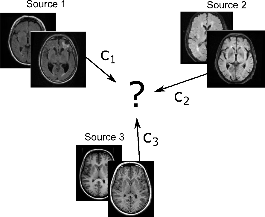
(a) Domain averaging of MRI scans’ sources.

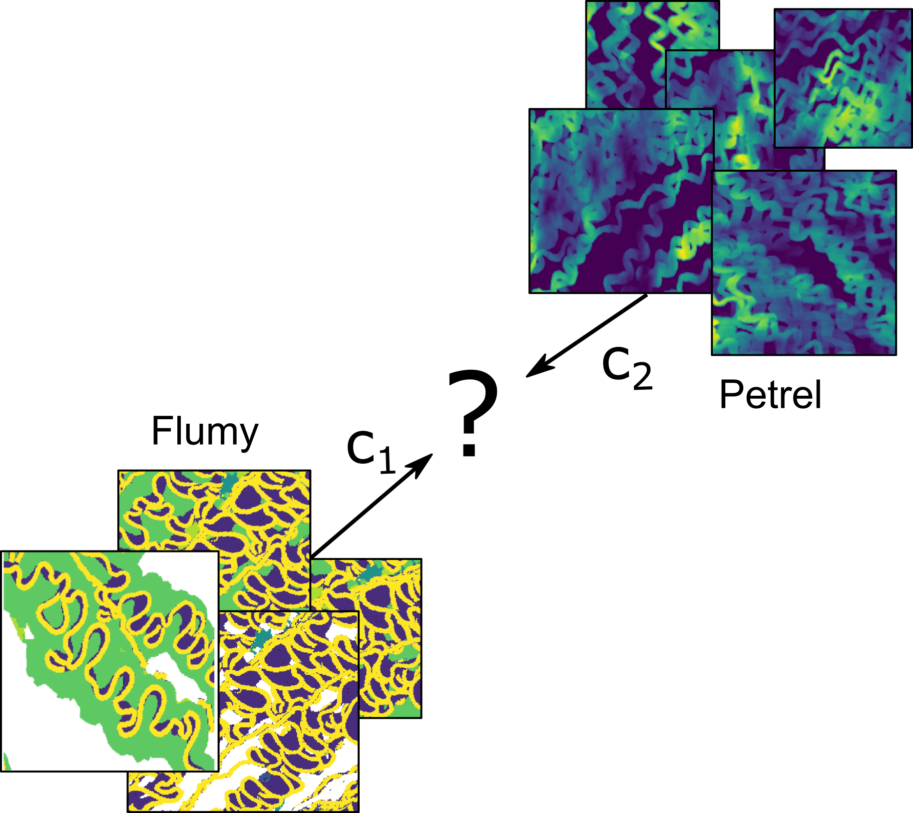
(b) Mixing geological simulators.

Figure 4: A schematical presentation of potential applications of barycenter solvers.

A potential way to overcome the above-mentioned limitations is to find a common representation of the data coming from multiple sources. This representation would require translation maps that can transform the new (previously unseen) data from each of the sources to this shared representation. This formulation closely aligns with the continuous barycenter learning setup (§2.3) studied in our paper. In this context, the barycenter could play the role of the shared representation.

To apply barycenters effectively to such domain averaging problems, two crucial ingredients are likely required: appropriate cost functions $c_{k}$ and a suitable data manifold $\mathcal{M}$ in which to search for the barycenters. The design of the cost itself may be a challenge requiring certain domain-specific knowledge that necessitates involving experts in the field. Meanwhile, the manifold constraint is required to avoid practically meaningless barycenters such as those considered in §5.2. Nowadays, with the rapid growth of the field of generative models, it is reasonable to expect that soon the new large models targeted for medical data may appear, analogously to DALL-E (Ramesh et al., 2022), StableDiffusion (Rombach et al., 2022) or StyleGAN-T (Sauer et al., 2023) for general image synthesis. These future models could potentially parameterize the medical data manifolds of interest, opening new possibilities for medical data analysis.

2. Mixing geological simulators (Fig. 4(b)). In geological modeling, variuos simulators exist to model different aspects of underground deposits. Sometimes one needs to build a generic tool which can take into account several desired geological factors which are successfully modeled by separate simulators.

Flumy is a process-based simulator that uses hydraulic theory (Ikeda et al., 1981) to model specific channel depositional processes returning a detailed three-dimensional geomodel informed with deposit lithotype, age and grain size. However, its result is a 3D segmentation field of facies (rock types) and it does not produce the real valued porosity field needed for hydrodynamical modeling.

Petrel software is the other popular simulator in the oil and gas industry. It is able to model complex real-valued geological maps such as the distribution of porosity. The produced porosity fields may not be realistic enough due to paying limited attention to the geological formation physics.

Both Flumy and Petrel simulators contain some level of stochasticity and are hard to use in conjunction. Even when conditioned on common prior information about the deposit, they may produce maps of facies and permeability which do not meaningfully correspond to each other. This limitation provides potential prospects for barycenter solvers which could be used to get the best from both simulators by mixing the distributions produced by each of them.

From our personal discussions with the experts in the field of geology, such task formulations are of considerable interest both for scientific community as well as industry. Applying our barycenter solver in this context is a challenge for future research. We acknowledge that this would also require overcoming considerable technical and domain-specific issues, including the data collection and the choice of costs $c_{k}$.

Appendix C Experimental Details

The hyper-parameters of our solver are summarized in Table 3. Some hyper-parameters, e.g., $L,S,iter$, are chosen primarily from time complexity reasons. Typically, the increase in these numbers positively affects the quality of the recovered solutions, see, e.g., (Gushchin et al., 2023b, Appendix E, Table 16). However, to reduce the computational burden, we report the figures which we found to be reasonable. Working with the manifold-constraint setup, we parameterize each $g_{\theta_{k}}(z)$ in our sover as $h_{\theta_{k}}\circ G(z)$, where $G$ is a pre-trained (frozen) StyleGAN and $h_{\theta_{k}}$ is a neural network with the ResNet architecture. We empirically found that this strategy provides better results than a direct MLP parameterization for the function $g_{\theta_{k}}(z)$.

Experiment	$D$	$K$	$\epsilon$	$\lambda_{1}$	$\lambda_{2}$	$\lambda_{3}$	$f_{\theta,k}$	$lr_{g_{\theta,k}}$	$iter$	$\sqrt{\eta}$	$L$	$S$
Toy 2D	2	3	$10^{-2}$	1/3	1/3	1/3	MLP	$10^{-2}$	200	1.0	300	256
MNIST 0/1	1024	2	$10^{-2}$	0.5	0.5	-	ResNet	$10^{-4}$	1000	0.1	500	32
MNIST 0/1	512	2	$10^{-2}$	0.5	0.5	-	ResNet	$10^{-4}$	1000	0.1	250	32
Ave, celeba!	512	3	$10^{-4}$	0.25	0.5	0.25	ResNet	$10^{-4}$	1000	0.1	250	128
Gaussians	2-64​	3	$10^{-2}$, 1	0.25	0.25	0.5	MLP	$10^{-3}$	50000	0.1	700	1024

Table 3: Hyperparameters that we use in the experiments with our algorithm 1.

To train the StyleGAN for MNSIT01 & Ave, celeba! experiments, we employ the official code from

https://github.com/NVlabs/stylegan2-ada-pytorch

C.1 Barycenters of 2D Distributions

Cartesian representation of twister map. In §5.1 we define twister map $u$ using polar coordinate system. For clearness, we give its form on cartesian coordinates. Let $x\in\mathbb{R}^{2}$, $x=(x_{(1)},x_{(2)})$. Note that $\|x\|=\sqrt{x_{(1)}^{2}+x_{(2)}^{2}}$ Then,

$$u(x)=u(x_{(1)},x_{(2)})=\begin{pmatrix}\cos\big{(}\|x\|\big{)}&-\sin\big{(}\|x\|\big{)}\\ \sin\big{(}\|x\|\big{)}&\cos\big{(}\|x\|\big{)}\end{pmatrix}\begin{pmatrix}x_{(1)}\\ x_{(2)}\end{pmatrix},$$

i.e., the twister map rotates input points $x$ by angles equal to $\|x\|$.

Analytical barycenter distribution for 2D Twister experiment. Below we provide a mathematical derivation that the true unregularized barycenter of the distributions $\mathbb{P}_{1},\mathbb{P}_{2},\mathbb{P}_{3}$ in Fig. 1(a) coincides with a Gaussian.

We begin with a rather general observation. Consider $\mathcal{X}_{k}=\mathcal{Y}=\mathbb{R}^{D}$ ($k\in\overline{K}$) and let $\text{OT}_{c}\stackrel{{\scriptstyle\text{def}}}{{=}}\text{EOT}_{c,0}$ denote the unregularized OT problem ($\epsilon=0$) for a given continuous cost function $c$. Let $u:\mathbb{R}^{D}\rightarrow\mathbb{R}^{D}$ be a measurable bijection and consider $\mathbb{P}_{k}^{\prime}\in\mathcal{P}(\mathbb{R}^{D})$ for $k\in\overline{K}$. By using the change of variables formula, we have for all $\mathbb{Q}^{\prime}\in\mathcal{P}(\mathbb{R}^{D})$ that

$$\text{OT}_{c\circ(u\times u)}(u^{-1}_{\#}(\mathbb{P}^{\prime}),u^{-1}_{\#}(\mathbb{Q}^{\prime}))=\text{OT}_{c}(\mathbb{P}^{\prime},\mathbb{Q}^{\prime}),$$ (56)

where $\#$ denotes the pushforward operator of distributions and $[c\circ(u\times u)](x,y)=c\big{(}u(x),u(y)\big{)}$. Note that by (56) the barycenter of $\mathbb{P}_{1}^{\prime},\dots,\mathbb{P}_{K}^{\prime}$ for the unregularized problem with cost $c$ coincides with the result of applying the pushforward operator $u^{-1}_{\#}$ to the barycenter of the very same problem but with cost $c\circ(u\times u)$.

Next, we fix $u$ to be the twister map (§5.1). In Fig. 1(a) we plot the distributions $\mathbb{P}_{1}\stackrel{{\scriptstyle\text{def}}}{{=}}u^{-1}_{\#}\mathbb{P}_{1}^{\prime},u^{-1}_{\#}\mathbb{P}_{1}^{\prime},u^{-1}_{\#}\mathbb{P}_{3}^{\prime}$ which are obtained from Gaussian distributions $\mathbb{P}_{1}^{\prime}=\mathcal{N}\big{(}(0,4),I_{2}\big{)},\mathbb{P}_{2}^{\prime}=\mathcal{N}\big{(}(-2,2\sqrt{3}),I_{2}\big{)},\mathbb{P}_{3}^{\prime}=\mathcal{N}\big{(}(2,2\sqrt{3}),I_{2}\big{)}$ by the pushforward. Here $I_{2}$ is the 2-dimensional identity matrix. For the unregularized $\ell^{2}$ barycenter problem, the barycenter of such shifted Gaussians can be derived analytically (Álvarez-Esteban et al., 2016). The solution coincides with a zero-centered standard Gaussian $\mathbb{Q}^{\prime}=\mathcal{N}\big{(}0,I_{2}\big{)}$. Hence, the barycenter of $\mathbb{P}_{1},\ldots,\mathbb{P}_{K}$ w.r.t. the cost $\ell^{2}\circ(u\times u)$ is given by $\mathbb{Q}^{*}=u^{-1}_{\#}\mathbb{Q}^{\prime}$. From the particular choice of $u$ it is not hard to see that ${\mathbb{Q}^{*}=\mathbb{Q}^{\prime}=\mathcal{N}\big{(}0,I_{2}\big{)}}$ as well.

C.2 Barycenters of MNIST Classes

Additional qualitative examples of our solver’s results are given in Figure 5.

Details of the baseline solvers. For the solver by (Fan et al., 2021, SCWB), we run their publicly available code from the official repository

https://github.com/sbyebss/Scalable-Wasserstein-Barycenter

The authors do no provide checkpoints, and we train their barycenter model from scratch. In turn, for the solver by (Korotin et al., 2022a, WIN), we also employ the publicly available code

https://github.com/iamalexkorotin/WassersteinIterativeNetworks

Here we do not train their models but just use the checkpoint available in their repo.

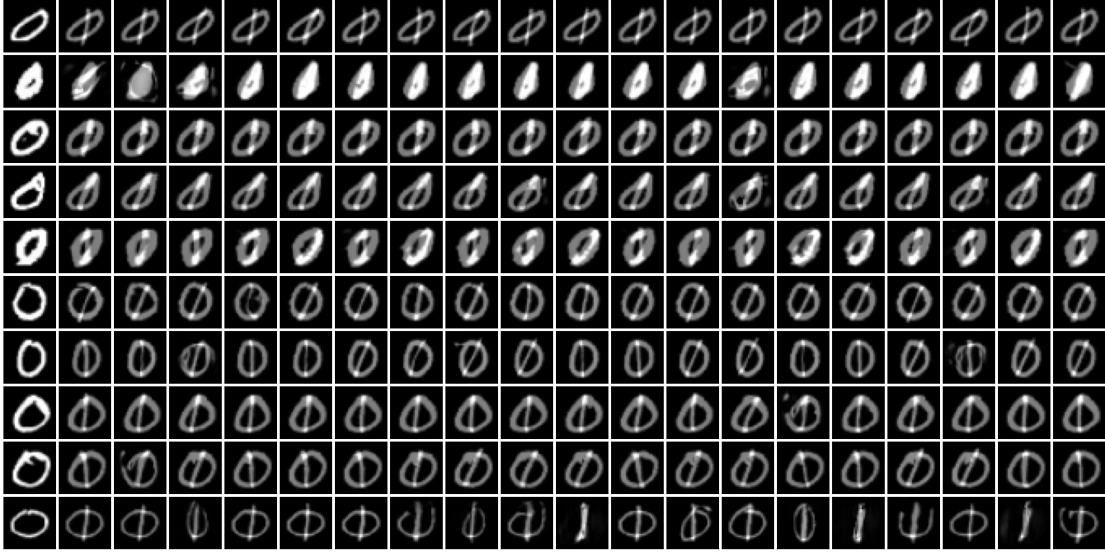
(a) Learned plans from $\mathbb{P}_{1}$ (zeros, 1st column) to the barycenter.

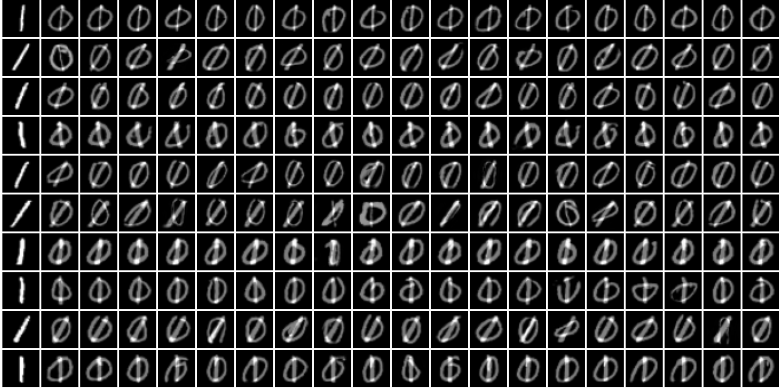
(b) Learned plans from $\mathbb{P}_{2}$ (ones, first column) to the barycenter.

Figure 5: Experiment with averaging MNIST 0/1 digit classes. The plot shows additional examples of samples transported with our solver to the barycenter.

C.3 Barycenters of the Ave,CELEBA! Dataset

Additional qualitative examples of our solver’s results are given in Figure 6.

Details of the baseline solvers. For the (Korotin et al., 2022a, WIN) solver, we use their pre-trained checkpoints provided by the authors in the above-mentioned repository. Note that the authors of (Fan et al., 2021, SCWB) do not consider such a high-dimensional setup with RGB images. Hence, to implement their approach in this setting, we follow (Korotin et al., 2022a, Appendix B.4).

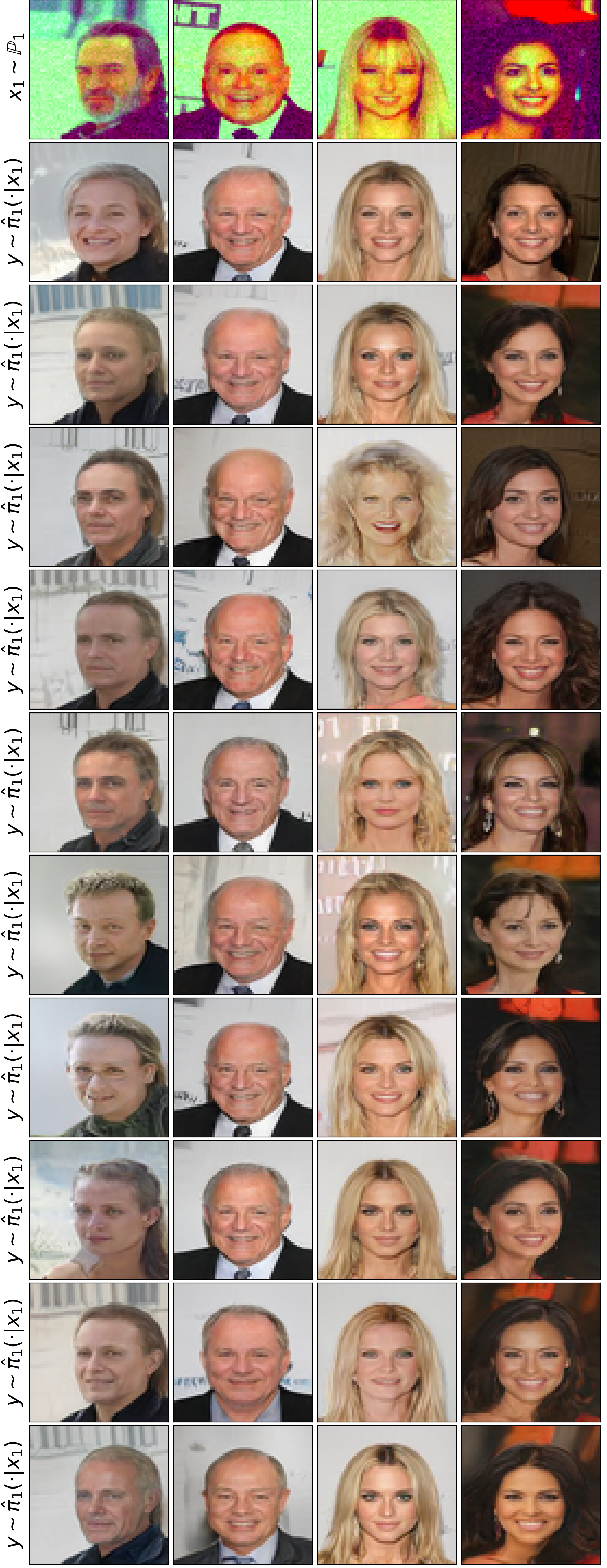
(a) Maps from $\mathbb{P}_{1}$ to the barycenter.

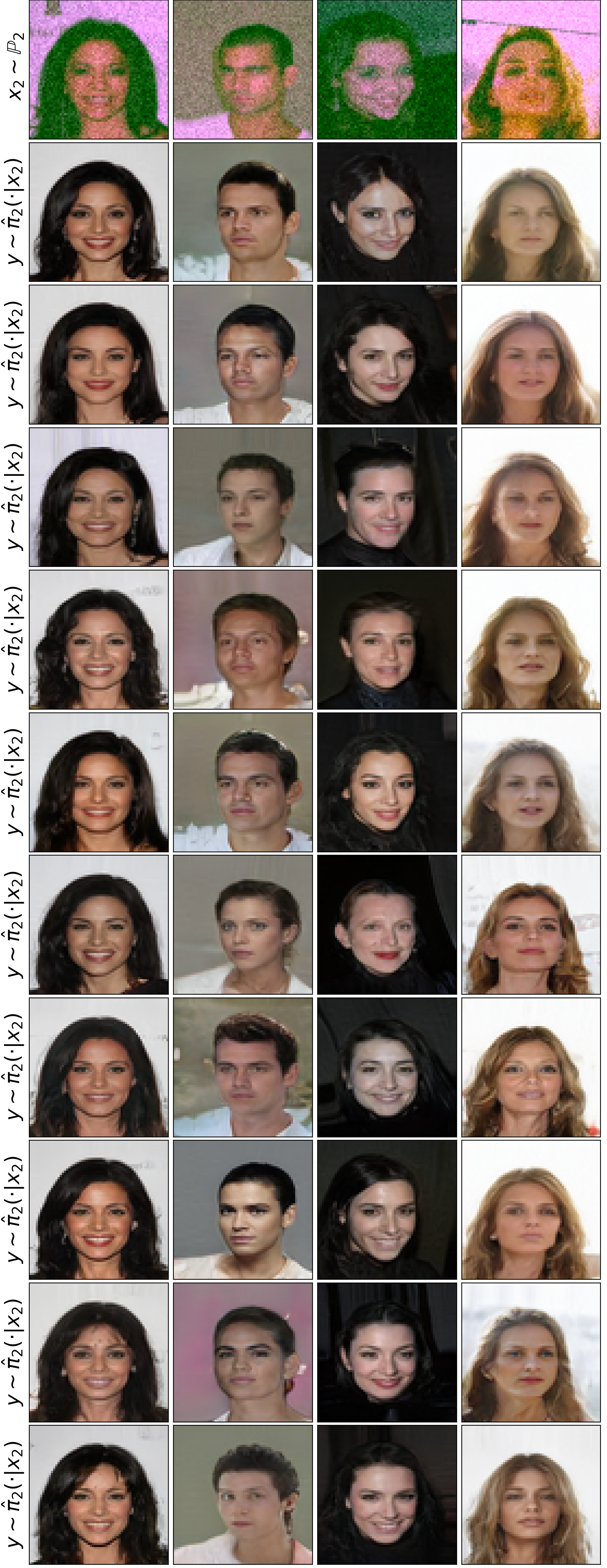
(b) Maps from $\mathbb{P}_{2}$ to the barycenter.

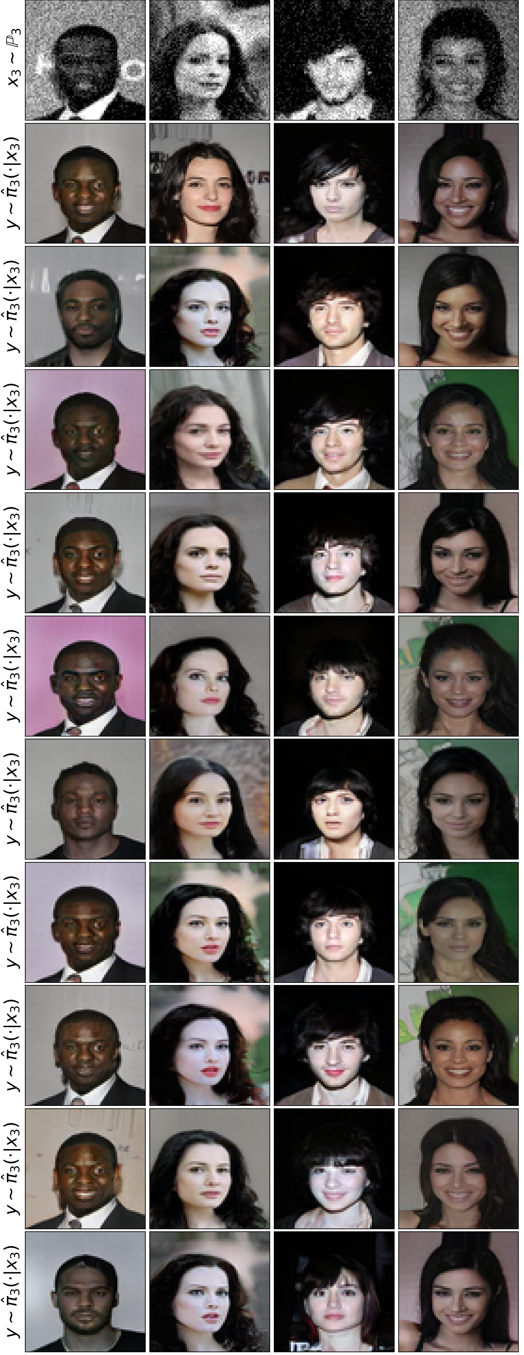
(c) Maps from $\mathbb{P}_{3}$ to the barycenter.

Figure 6: Experiment on the Ave, celeba! barycenter dataset. The plots show additional examples of samples transported with our solver to the barycenter.

C.4 Barycenters of Gaussian Distributions

We note that there exist many ways to incorporate the entropic regularization for barycenters (Chizat, 2023, Table 1); these problems do not coincide and yield different solutions. For some of them, the ground-truth solutions are known for specific cases such as the Gaussian case. For example, (Mallasto et al., 2022, Theorem 3) examines barycenters for OT regularized with KL divergence. They consider the task

$$\inf_{\mathbb{Q}\in\mathcal{P(Y)}}\sum_{k=1}^{K}\lambda_{k}\big{(}\int_{\mathcal{X}\times\mathcal{Y}}\frac{\|x-y\|^{2}}{2}d\pi_{k}(x,y)+\epsilon\text{KL}(\pi_{k}\|\mathbb{P}_{k}\times\mathbb{Q})\big{)}=$$

$$\inf_{\mathbb{Q}\in\mathcal{P(Y)}}\sum_{k=1}^{K}\lambda_{k}\big{(}\int_{\mathcal{X}\times\mathcal{Y}}\frac{\|x-y\|^{2}}{2}d\pi_{k}(x,y)-\epsilon\int_{\mathcal{X}}H(\pi_{k}(\cdot|x))d\mathbb{P}_{k}(x)+\epsilon H(\mathbb{Q})\big{)}=$$

$$\inf_{\mathbb{Q}\in\mathcal{P(Y)}}\bigg{\{}\underbrace{\sum_{k=1}^{K}\lambda_{k}\text{EOT}^{(2)}_{\ell^{2},\epsilon}(\mathbb{P}_{k},\mathbb{Q})}_{=\text{ our objective inside }\eqref{EOT_bary_primal_alternative}}+\epsilon H(\mathbb{Q})\bigg{\}}.$$

This problem differs from our objective (7) with $c(x,y)=\frac{1}{2}\|x-y\|^{2}$ by the non-constant $\mathbb{Q}$-dependent term $\epsilon H(\mathbb{Q})$; this problem yields a different solution. The difference of other mentioned approaches can be shown in the same way. In particular, (Le et al., 2022) tackles the barycenter for inner product Gromov-Wasserstein problem with entropic regularization which is not relevant for us. To our knowledge, the Gaussian ground-truth solution for our problem setup (7) is not yet known, although some of its properties seem to be established (del Barrio & Loubes, 2020).

Still when $\epsilon\approx 0$, our entropy-regularized barycenter is expected to be close to the unregularized one ($\epsilon=0$). In the Gaussian case, it is known that the unregularized OT barycenter for $c_{k}(x,y)=\frac{1}{2}\|x-y\|^{2}$ is itself Gaussian and can be computed using the well-celebrated fixed point iterations of (Álvarez-Esteban et al., 2016, Eq. (19)). This gives us an opportunity to compare our results with the ground-truth unregularized barycenter in the Gaussian case. As the baseline, we include the results of (Korotin et al., 2022a, WIN) solver which learns the unregularized barycenter (${\epsilon}=0$).

We consider 3 Gaussian distributions $\mathbb{P}_{1},\mathbb{P}_{2},\mathbb{P}_{3}$ in dimensions $D=2,4,8,16,64$ and compute the approximate EOT barycenters $\pi^{\widehat{f}_{k}}_{k}$ for $\epsilon=0.01,1$ w.r.t. weights $(\lambda_{1},\lambda_{2},\lambda_{3})=(\frac{1}{4},\frac{1}{4},\frac{1}{2})$ with our solver. To initialize these distributions, we follow the strategy of (Korotin et al., 2022a, Appendix C.2). The ground truth unregularized barycenter $\mathbb{Q}^{*}$ is estimated via the above-mentioned iterative procedure. We use the code from WIN repository available via the link mentioned in Appendix C.2. To assess the WIN solver, we use the unexplained variance percentage metrics defined as $\mathcal{L}_{2}\text{-UVP}(\hat{T})=100\cdot[\|\hat{T}-T^{*}\|]_{\mathbb{P}}^{2}$ where $T^{*}$ denotes the optimal transport map $T^{*}$, see (Korotin et al., 2021a, §5.1). Since our solver computes EOT plans but not maps, we evaluate the barycentric projections of the learned plans, i.e., $\widehat{\overline{T}}_{k}(x)=\int_{\mathcal{Y}}y\pi_{k}^{\widehat{f}_{k}}(y|x)$, and calculate $\mathcal{L}_{2}\text{-UVP}(\widehat{\overline{T}}_{k},T^{*}_{k})$. We evaluate this metric using $10^{4}$ samples. To estimate the barycentric projection in our solver, we use $10^{3}$ samples $y\sim\pi_{k}^{\widehat{f}_{k}}(y|x_{k})$ for each $x_{k}$. To keep the table with the results simple, in each case we report the average of this metric for $k=1,2,3$ w.r.t. the weights $\lambda_{k}$.

Dim / Method	Ours (${\epsilon}=1$)	Ours (${\epsilon}=0.01$)	(Korotin et al., 2022a, WIN)
2	1.12	0.02	0.03
4	1.6	0.05	0.08
8	1.85	0.06	0.13
16	1.32	0.09	0.25
64	1.83	0.84	0.75

Table 4: $\mathcal{L}_{2}\text{-UVP}$ for our method with ${\epsilon}=0.01,1$ and WIN, $D=2,4,8,16,64$.

Results. We see that for small ${\epsilon}=0.01$ and dimension up to $D=16$, our algorithm gives the results even better than WIN solver designed specifically for the unregularized case ($\epsilon=0$). As was expected, larger ${\epsilon}=1$ leads to the increased bias in the solutions of our algorithm and $\mathcal{L}_{2}\text{-UVP}$ metric increases.

Appendix D Alternative EBM training procedure

(a) The true unregularized barycenter for the twisted cost.

(b) Our EOT barycenter for the twisted cost (map from $\mathbb{P}_{1}$).

(c) The true unregularized barycenter for $\ell^{2}$ cost.

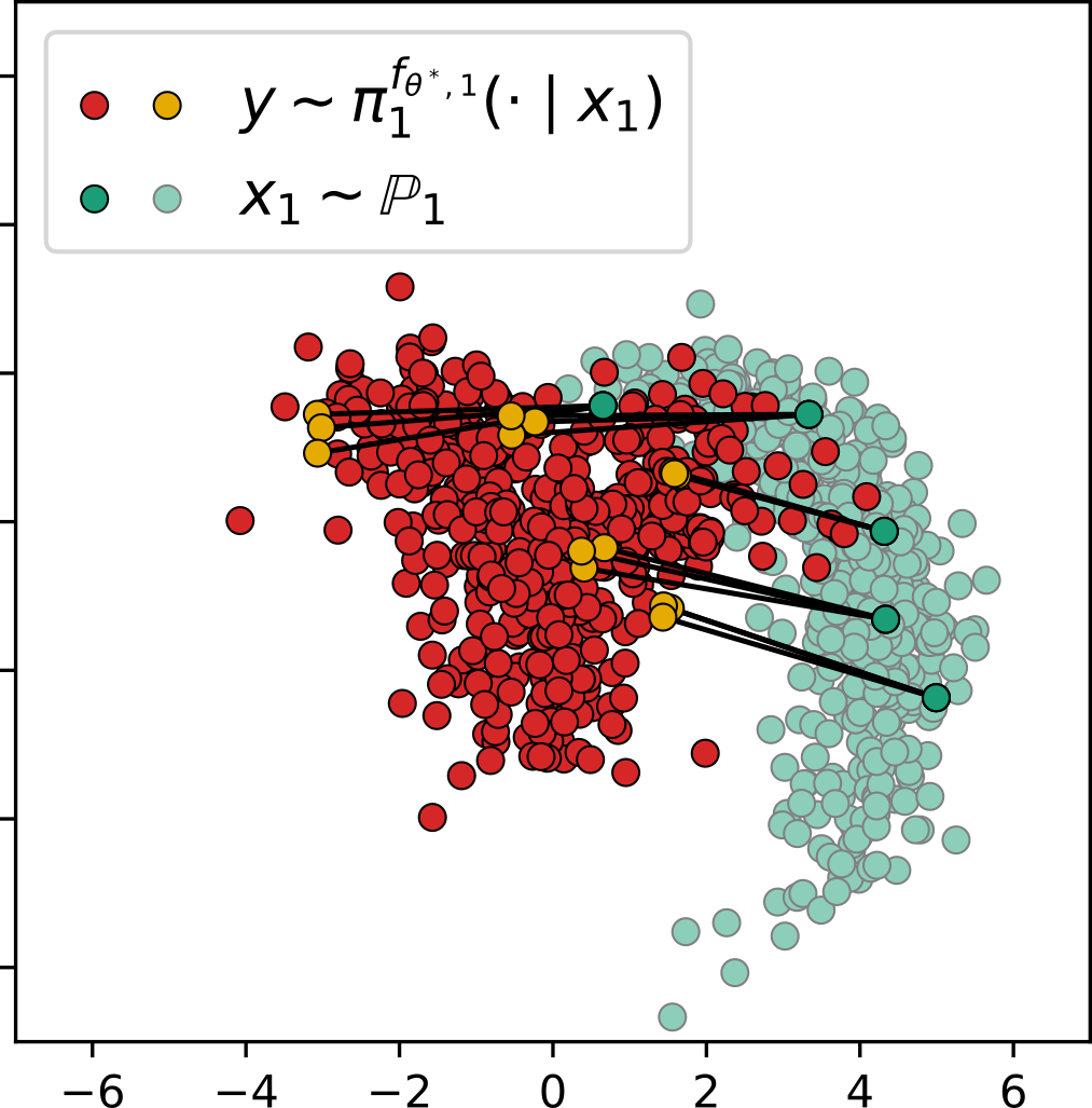
(d) Our EOT barycenter for $\ell^{2}$ cost (map from $\mathbb{P}_{1}$).

Figure 7: 2D twister example. Trained with importance sampling: The true barycenter of 3 comets vs. the one computed by our solver with ${\epsilon}=10^{-2}$. Two costs $c_{k}$ are considered: the twisted cost (7(a), 7(b)) and $\ell^{2}$ (7(c), 7(d)). We employ the simulation-free importance sampling procedure for training.

In this section, we describe an alternative simulation-free training procedure for learning EOT barycenter distribution via our proposed methodology. The key challenge behind our approach is to estimate the gradient of the dual objective (4.3). To overcome the difficulty, in the main part of our manuscript, we utilize MCMC sampling from conditional distributions $\mu_{x_{k}}^{f_{\theta,k}}$ and estimate the loss with Monte-Carlo. Here we discuss a potential alternative approach based on importance sampling (IS) (Tokdar & Kass, 2010). That is, we evaluate the internal integral over $\mathcal{Y}$ in (4.3):

$$\mathcal{I}(x_{k})\stackrel{{\scriptstyle\text{def}}}{{=}}\int_{\mathcal{Y}}\left[\frac{\partial}{\partial\theta}f_{\theta,k}(y)\right]\mathrm{d}\mu_{x_{k}}^{f_{\theta,k}}(y)$$ (57)

with help of an auxiliary proposal (continuous) distribution accessible by samples with the known density $q(y)$. Let $Y^{q}=\{y_{1}^{q},\dots,y_{P}^{q}\}$ be a sample from $q(y)$. Define the weights:

$$\omega_{k}(x_{k},y_{p}^{q})\stackrel{{\scriptstyle\text{def}}}{{=}}\exp\bigg{(}\frac{f_{\theta,k}(y_{p}^{q})-c(x_{k},y_{p}^{q})}{\varepsilon}\bigg{)}q(y_{p}^{q}).$$

Then (57) permits the following stochastic estimate:

$$\mathcal{I}(x_{k})\approx\frac{\sum\nolimits_{p=1}^{P}\left[\frac{\partial}{\partial\theta}f_{\theta,k}(y)\right]\omega_{k}(x_{k},y_{p}^{q})}{\sum\nolimits_{p=1}^{P}\omega_{k}(x_{k},y_{p}^{q})}.$$ (58)

Experimental illustration. To demonstrate the applicability of IS-based training procedure to our barycenter setting, we conduct the experiment following our 2D Twister setup, see §5.1. We employ zero-mean $16I$-covariance Gaussian distribution as $q$ and pick the batch size $P=1024$. Our results are shown in Figure 7. As we can see, the alternative training procedure yields similar results to Figure1 but converges faster ($\approx 1$ min. VS $\approx 18$ min. of the original MCMC-based training).

Concluding remarks. We note that IS-based methods requires accurate selection of the proposal distribution $q$ to reduce the variance of the estimator (Tokdar & Kass, 2010). It may be challenging in real-world scenarios. We leave the detailed study of more advanced IS approaches in the context of energy-based models and their applicability to our EOT barycentric setup to follow-up research.

References

- Agueh & Carlier (2011) Agueh, M. and Carlier, G. Barycenters in the wasserstein space. SIAM Journal on Mathematical Analysis, 43(2):904–924, 2011.
- Altschuler & Boix-Adsera (2022) Altschuler, J. M. and Boix-Adsera, E. Wasserstein barycenters are np-hard to compute. SIAM Journal on Mathematics of Data Science, 4(1):179–203, 2022.
- Álvarez-Esteban et al. (2016) Álvarez-Esteban, P. C., Del Barrio, E., Cuesta-Albertos, J., and Matrán, C. A fixed-point approach to barycenters in wasserstein space. Journal of Mathematical Analysis and Applications, 441(2):744–762, 2016.
- Ambrosio & Gigli (2013) Ambrosio, L. and Gigli, N. A User’s Guide to Optimal Transport, pp. 1–155. Springer Berlin Heidelberg, Berlin, Heidelberg, 2013. ISBN 978-3-642-32160-3. doi: 10.1007/978-3-642-32160-3˙1. URL https://doi.org/10.1007/978-3-642-32160-3_1.
- Amos (2022) Amos, B. On amortizing convex conjugates for optimal transport. In The Eleventh International Conference on Learning Representations, 2022.
- Amos et al. (2017) Amos, B., Xu, L., and Kolter, J. Z. Input convex neural networks. In International Conference on Machine Learning, pp. 146–155. PMLR, 2017.
- Andrieu et al. (2003) Andrieu, C., De Freitas, N., Doucet, A., and Jordan, M. I. An introduction to mcmc for machine learning. Machine learning, 50:5–43, 2003.
- Asadulaev et al. (2024) Asadulaev, A., Korotin, A., Egiazarian, V., and Burnaev, E. Neural optimal transport with general cost functionals. In The Twelfth International Conference on Learning Representations, 2024.
- Backhoff-Veraguas et al. (2019) Backhoff-Veraguas, J., Beiglböck, M., and Pammer, G. Existence, duality, and cyclical monotonicity for weak transport costs. Calculus of Variations and Partial Differential Equations, 58(6):203, 2019.
- Bartlett & Mendelson (2002) Bartlett, P. L. and Mendelson, S. Rademacher and Gaussian complexities: risk bounds and structural results. J. Mach. Learn. Res., 3:463–482, 2002. ISSN 1532-4435,1533-7928. doi: 10.1162/153244303321897690. URL https://doi.org/10.1162/153244303321897690.
- Benamou et al. (2015) Benamou, J.-D., Carlier, G., Cuturi, M., Nenna, L., and Peyré, G. Iterative bregman projections for regularized transportation problems. SIAM Journal on Scientific Computing, 37(2):A1111–A1138, 2015.
- Cazelles et al. (2021) Cazelles, E., Tobar, F., and Fontbona, J. A novel notion of barycenter for probability distributions based on optimal weak mass transport. Advances in Neural Information Processing Systems, 34:13575–13586, 2021.
- Chen et al. (2021) Chen, T., Liu, G.-H., and Theodorou, E. A. Likelihood training of schr” odinger bridge using forward-backward sdes theory. arXiv preprint arXiv:2110.11291, 2021.
- Chi et al. (2023) Chi, J., Yang, Z., Li, X., Ouyang, J., and Guan, R. Variational wasserstein barycenters with c-cyclical monotonicity regularization. In Proceedings of the AAAI Conference on Artificial Intelligence, volume 37, pp. 7157–7165, 2023.
- Chizat (2023) Chizat, L. Doubly regularized entropic wasserstein barycenters. arXiv preprint arXiv:2303.11844, 2023.
- Clason et al. (2021) Clason, C., Lorenz, D. A., Mahler, H., and Wirth, B. Entropic regularization of continuous optimal transport problems. Journal of Mathematical Analysis and Applications, 494(1):124432, 2021.
- Cohen et al. (2020) Cohen, S., Arbel, M., and Deisenroth, M. P. Estimating barycenters of measures in high dimensions. arXiv preprint arXiv:2007.07105, 2020.
- Colombo et al. (2021) Colombo, P., Staerman, G., Clavel, C., and Piantanida, P. Automatic text evaluation through the lens of Wasserstein barycenters. In Proceedings of the 2021 Conference on Empirical Methods in Natural Language Processing, pp. 10450–10466, Online and Punta Cana, Dominican Republic, November 2021. Association for Computational Linguistics. doi: 10.18653/v1/2021.emnlp-main.817. URL https://aclanthology.org/2021.emnlp-main.817.
- Cuturi (2013) Cuturi, M. Sinkhorn distances: Lightspeed computation of optimal transport. In Burges, C., Bottou, L., Welling, M., Ghahramani, Z., and Weinberger, K. (eds.), Advances in Neural Information Processing Systems, volume 26. Curran Associates, Inc., 2013. URL https://proceedings.neurips.cc/paper_files/paper/2013/file/af21d0c97db2e27e13572cbf59eb343d-Paper.pdf.
- Cuturi & Doucet (2014) Cuturi, M. and Doucet, A. Fast computation of wasserstein barycenters. In International conference on machine learning, pp. 685–693. PMLR, 2014.
- Cuturi & Peyré (2016) Cuturi, M. and Peyré, G. A smoothed dual approach for variational wasserstein problems. SIAM Journal on Imaging Sciences, 9(1):320–343, 2016.
- Cuturi & Peyré (2018) Cuturi, M. and Peyré, G. Semidual regularized optimal transport. SIAM Review, 60(4):941–965, 2018. doi: 10.1137/18M1208654.
- Daniels et al. (2021) Daniels, M., Maunu, T., and Hand, P. Score-based generative neural networks for large-scale optimal transport. Advances in neural information processing systems, 34:12955–12965, 2021.
- De Bortoli et al. (2021) De Bortoli, V., Thornton, J., Heng, J., and Doucet, A. Diffusion schrödinger bridge with applications to score-based generative modeling. Advances in Neural Information Processing Systems, 34:17695–17709, 2021.
- del Barrio & Loubes (2020) del Barrio, E. and Loubes, J.-M. The statistical effect of entropic regularization in optimal transportation, 2020.
- Du & Mordatch (2019) Du, Y. and Mordatch, I. Implicit generation and modeling with energy based models. Advances in Neural Information Processing Systems, 32, 2019.
- Du et al. (2021) Du, Y., Li, S., Tenenbaum, B. J., and Mordatch, I. Improved contrastive divergence training of energy based models. In Proceedings of the 38th International Conference on Machine Learning (ICML-21), 2021.
- Du et al. (2023) Du, Y., Durkan, C., Strudel, R., Tenenbaum, J. B., Dieleman, S., Fergus, R., Sohl-Dickstein, J., Doucet, A., and Grathwohl, W. S. Reduce, reuse, recycle: Compositional generation with energy-based diffusion models and mcmc. In International Conference on Machine Learning, pp. 8489–8510. PMLR, 2023.
- Dugundji (1951) Dugundji, J. An extension of Tietze’s theorem. Pacific J. Math., 1:353–367, 1951. ISSN 0030-8730,1945-5844. URL http://projecteuclid.org/euclid.pjm/1103052106.
- Dvurechenskii et al. (2018) Dvurechenskii, P., Dvinskikh, D., Gasnikov, A., Uribe, C., and Nedich, A. Decentralize and randomize: Faster algorithm for wasserstein barycenters. Advances in Neural Information Processing Systems, 31, 2018.
- Fan et al. (2021) Fan, J., Taghvaei, A., and Chen, Y. Scalable computations of wasserstein barycenter via input convex neural networks. In Meila, M. and Zhang, T. (eds.), Proceedings of the 38th International Conference on Machine Learning, volume 139 of Proceedings of Machine Learning Research, pp. 1571–1581. PMLR, 18–24 Jul 2021. URL https://proceedings.mlr.press/v139/fan21d.html.
- Flamary et al. (2021) Flamary, R., Courty, N., Gramfort, A., Alaya, M. Z., Boisbunon, A., Chambon, S., Chapel, L., Corenflos, A., Fatras, K., Fournier, N., Gautheron, L., Gayraud, N. T., Janati, H., Rakotomamonjy, A., Redko, I., Rolet, A., Schutz, A., Seguy, V., Sutherland, D. J., Tavenard, R., Tong, A., and Vayer, T. Pot: Python optimal transport. Journal of Machine Learning Research, 22(78):1–8, 2021. URL http://jmlr.org/papers/v22/20-451.html.
- Gao et al. (2021) Gao, R., Song, Y., Poole, B., Wu, Y. N., and Kingma, D. P. Learning energy-based models by diffusion recovery likelihood. In International Conference on Learning Representations, 2021. URL https://openreview.net/forum?id=v_1Soh8QUNc.
- Gazdieva et al. (2023) Gazdieva, M., Korotin, A., Selikhanovych, D., and Burnaev, E. Extremal domain translation with neural optimal transport. In Advances in Neural Information Processing Systems, 2023.
- Genevay (2019) Genevay, A. Entropy-regularized optimal transport for machine learning. PhD thesis, Paris Sciences et Lettres (ComUE), 2019.
- Genevay et al. (2016) Genevay, A., Cuturi, M., Peyré, G., and Bach, F. Stochastic optimization for large-scale optimal transport. Advances in neural information processing systems, 29, 2016.
- Gottlieb et al. (2016) Gottlieb, L.-A., Kontorovich, A., and Krauthgamer, R. Adaptive metric dimensionality reduction. volume 620, pp. 105–118. 2016. doi: 10.1016/j.tcs.2015.10.040. URL https://doi.org/10.1016/j.tcs.2015.10.040.
- Gozlan et al. (2017) Gozlan, N., Roberto, C., Samson, P.-M., and Tetali, P. Kantorovich duality for general transport costs and applications. Journal of Functional Analysis, 273(11):3327–3405, 2017.
- Guan & Liu (2021) Guan, H. and Liu, M. Domain adaptation for medical image analysis: a survey. IEEE Transactions on Biomedical Engineering, 69(3):1173–1185, 2021.
- Gushchin et al. (2023a) Gushchin, N., Kolesov, A., Korotin, A., Vetrov, D., and Burnaev, E. Entropic neural optimal transport via diffusion processes. In Advances in Neural Information Processing Systems, 2023a.
- Gushchin et al. (2023b) Gushchin, N., Kolesov, A., Mokrov, P., Karpikova, P., Spiridonov, A., Burnaev, E., and Korotin, A. Building the bridge of schr” odinger: A continuous entropic optimal transport benchmark. In Thirty-seventh Conference on Neural Information Processing Systems Datasets and Benchmarks Track, 2023b.
- Habib & Barber (2018) Habib, R. and Barber, D. Auxiliary variational mcmc. In International Conference on Learning Representations, 2018.
- Henry-Labordere (2019) Henry-Labordere, P. (martingale) optimal transport and anomaly detection with neural networks: A primal-dual algorithm. arXiv preprint arXiv:1904.04546, 2019.
- Heusel et al. (2017) Heusel, M., Ramsauer, H., Unterthiner, T., Nessler, B., and Hochreiter, S. Gans trained by a two time-scale update rule converge to a local nash equilibrium. Advances in neural information processing systems, 30, 2017.
- Hinton (2002) Hinton, G. E. Training products of experts by minimizing contrastive divergence. Neural computation, 14(8):1771–1800, 2002.
- Hoffman et al. (2019) Hoffman, M., Sountsov, P., Dillon, J. V., Langmore, I., Tran, D., and Vasudevan, S. Neutra-lizing bad geometry in hamiltonian monte carlo using neural transport. arXiv preprint arXiv:1903.03704, 2019.
- Ikeda et al. (1981) Ikeda, S., Parker, G., and Sawai, K. Bend theory of river meanders. part 1. linear development. Journal of Fluid Mechanics, 112:363–377, 1981.
- Kantorovich (1942) Kantorovich, L. V. On the translocation of masses. In Dokl. Akad. Nauk. USSR (NS), volume 37, pp. 199–201, 1942.
- Karras et al. (2019) Karras, T., Laine, S., and Aila, T. A style-based generator architecture for generative adversarial networks. In Proceedings of the IEEE/CVF conference on computer vision and pattern recognition, pp. 4401–4410, 2019.
- Kondrateva et al. (2021) Kondrateva, E., Pominova, M., Popova, E., Sharaev, M., Bernstein, A., and Burnaev, E. Domain shift in computer vision models for mri data analysis: an overview. In Thirteenth International Conference on Machine Vision, volume 11605, pp. 126–133. SPIE, 2021.
- Korotin et al. (2021a) Korotin, A., Egiazarian, V., Asadulaev, A., Safin, A., and Burnaev, E. Wasserstein-2 generative networks. In International Conference on Learning Representations, 2021a.
- Korotin et al. (2021b) Korotin, A., Li, L., Genevay, A., Solomon, J. M., Filippov, A., and Burnaev, E. Do neural optimal transport solvers work? a continuous wasserstein-2 benchmark. Advances in Neural Information Processing Systems, 34:14593–14605, 2021b.
- Korotin et al. (2021c) Korotin, A., Li, L., Solomon, J., and Burnaev, E. Continuous wasserstein-2 barycenter estimation without minimax optimization. In International Conference on Learning Representations, 2021c. URL https://openreview.net/forum?id=3tFAs5E-Pe.
- Korotin et al. (2022a) Korotin, A., Egiazarian, V., Li, L., and Burnaev, E. Wasserstein iterative networks for barycenter estimation. In Oh, A. H., Agarwal, A., Belgrave, D., and Cho, K. (eds.), Advances in Neural Information Processing Systems, 2022a. URL https://openreview.net/forum?id=GiEnzxTnaMN.
- Korotin et al. (2022b) Korotin, A., Kolesov, A., and Burnaev, E. Kantorovich strikes back! wasserstein gans are not optimal transport? Advances in Neural Information Processing Systems, 35:13933–13946, 2022b.
- Korotin et al. (2023a) Korotin, A., Selikhanovych, D., and Burnaev, E. Kernel neural optimal transport. In The Eleventh International Conference on Learning Representations, 2023a.
- Korotin et al. (2023b) Korotin, A., Selikhanovych, D., and Burnaev, E. Neural optimal transport. In The Eleventh International Conference on Learning Representations, 2023b.
- Kratsios & Papon (2022) Kratsios, A. and Papon, L. Universal approximation theorems for differentiable geometric deep learning. J. Mach. Learn. Res., 23:Paper No. [196], 73, 2022. ISSN 1532-4435,1533-7928.
- Krawtschenko et al. (2020) Krawtschenko, R., Uribe, C. A., Gasnikov, A., and Dvurechensky, P. Distributed optimization with quantization for computing wasserstein barycenters. arXiv preprint arXiv:2010.14325, 2020.
- Kroshnin et al. (2019) Kroshnin, A., Tupitsa, N., Dvinskikh, D., Dvurechensky, P., Gasnikov, A., and Uribe, C. On the complexity of approximating wasserstein barycenters. In International conference on machine learning, pp. 3530–3540. PMLR, 2019.
- Kushol et al. (2023) Kushol, R., Wilman, A. H., Kalra, S., and Yang, Y.-H. Dsmri: Domain shift analyzer for multi-center mri datasets. Diagnostics, 13(18):2947, 2023.
- Lawson et al. (2019) Lawson, J., Tucker, G., Dai, B., and Ranganath, R. Energy-inspired models: Learning with sampler-induced distributions. Advances in Neural Information Processing Systems, 32, 2019.
- Le et al. (2021) Le, K., Nguyen, H., Nguyen, Q. M., Pham, T., Bui, H., and Ho, N. On robust optimal transport: Computational complexity and barycenter computation. Advances in Neural Information Processing Systems, 34:21947–21959, 2021.
- Le et al. (2022) Le, K., Le, D. Q., Nguyen, H., Do, D., Pham, T., and Ho, N. Entropic gromov-wasserstein between gaussian distributions. In International Conference on Machine Learning, pp. 12164–12203. PMLR, 2022.
- LeCun et al. (2006) LeCun, Y., Chopra, S., Hadsell, R., Ranzato, M., and Huang, F. A tutorial on energy-based learning. Predicting structured data, 1(0), 2006.
- Léonard (2013) Léonard, C. A survey of the schrödinger problem and some of its connections with optimal transport. Discrete and Continuous Dynamical Systems, 34(4):1533–1574, 2013.
- Levy et al. (2017) Levy, D., Hoffman, M. D., and Sohl-Dickstein, J. Generalizing hamiltonian monte carlo with neural networks. arXiv preprint arXiv:1711.09268, 2017.
- Li et al. (2020) Li, L., Genevay, A., Yurochkin, M., and Solomon, J. M. Continuous regularized wasserstein barycenters. Advances in Neural Information Processing Systems, 33:17755–17765, 2020.
- Liu et al. (2015) Liu, Z., Luo, P., Wang, X., and Tang, X. Deep learning face attributes in the wild. In Proceedings of International Conference on Computer Vision (ICCV), December 2015.
- Makkuva et al. (2020) Makkuva, A., Taghvaei, A., Oh, S., and Lee, J. Optimal transport mapping via input convex neural networks. In International Conference on Machine Learning, pp. 6672–6681. PMLR, 2020.
- Mallasto et al. (2022) Mallasto, A., Gerolin, A., and Minh, H. Q. Entropy-regularized 2-wasserstein distance between gaussian measures. Information Geometry, 5(1):289–323, 2022.
- Marino & Gerolin (2020) Marino, S. D. and Gerolin, A. An optimal transport approach for the schrödinger bridge problem and convergence of sinkhorn algorithm. Journal of Scientific Computing, 85(2):27, 2020.
- Metelli et al. (2019) Metelli, A. M., Likmeta, A., and Restelli, M. Propagating uncertainty in reinforcement learning via wasserstein barycenters. Advances in Neural Information Processing Systems, 32, 2019.
- Mokrov et al. (2024) Mokrov, P., Korotin, A., Kolesov, A., Gushchin, N., and Burnaev, E. Energy-guided entropic neural optimal transport. In The Twelfth International Conference on Learning Representations, 2024. URL https://openreview.net/forum?id=d6tUsZeVs7.
- Montesuma & Mboula (2021) Montesuma, E. F. and Mboula, F. M. N. Wasserstein barycenter for multi-source domain adaptation. In Proceedings of the IEEE/CVF conference on computer vision and pattern recognition, pp. 16785–16793, 2021.
- Mroueh (2020) Mroueh, Y. Wasserstein style transfer. In Chiappa, S. and Calandra, R. (eds.), Proceedings of the Twenty Third International Conference on Artificial Intelligence and Statistics, volume 108 of Proceedings of Machine Learning Research, pp. 842–852. PMLR, 26–28 Aug 2020. URL https://proceedings.mlr.press/v108/mroueh20a.html.
- Neklyudov et al. (2020) Neklyudov, K., Welling, M., Egorov, E., and Vetrov, D. Involutive mcmc: a unifying framework. In International Conference on Machine Learning, pp. 7273–7282. PMLR, 2020.
- Noble et al. (2023) Noble, M., De Bortoli, V., Doucet, A., and Durmus, A. Tree-based diffusion schr” odinger bridge with applications to wasserstein barycenters. arXiv preprint arXiv:2305.16557, 2023.
- Peyré et al. (2019) Peyré, G., Cuturi, M., et al. Computational optimal transport: With applications to data science. Foundations and Trends® in Machine Learning, 11(5-6):355–607, 2019.
- Ramesh et al. (2022) Ramesh, A., Dhariwal, P., Nichol, A., Chu, C., and Chen, M. Hierarchical text-conditional image generation with clip latents. arXiv preprint arXiv:2204.06125, 1(2):3, 2022.
- Roberts & Tweedie (1996) Roberts, G. O. and Tweedie, R. L. Exponential convergence of langevin distributions and their discrete approximations. Bernoulli, pp. 341–363, 1996.
- Rombach et al. (2022) Rombach, R., Blattmann, A., Lorenz, D., Esser, P., and Ommer, B. High-resolution image synthesis with latent diffusion models. In Proceedings of the IEEE/CVF conference on computer vision and pattern recognition, pp. 10684–10695, 2022.
- Rout et al. (2021) Rout, L., Korotin, A., and Burnaev, E. Generative modeling with optimal transport maps. In International Conference on Learning Representations, 2021.
- Santambrogio (2015) Santambrogio, F. Optimal transport for applied mathematicians. Birkäuser, NY, 55(58-63):94, 2015.
- Sauer et al. (2023) Sauer, A., Karras, T., Laine, S., Geiger, A., and Aila, T. Stylegan-t: Unlocking the power of gans for fast large-scale text-to-image synthesis. arXiv preprint arXiv:2301.09515, 2023.
- Seguy et al. (2018) Seguy, V., Damodaran, B. B., Flamary, R., Courty, N., Rolet, A., and Blondel, M. Large scale optimal transport and mapping estimation. In International Conference on Learning Representations, 2018. URL https://openreview.net/forum?id=B1zlp1bRW.
- Sejdinovic et al. (2014) Sejdinovic, D., Strathmann, H., Garcia, M. L., Andrieu, C., and Gretton, A. Kernel adaptive metropolis-hastings. In International conference on machine learning, pp. 1665–1673. PMLR, 2014.
- Shalev-Shwartz & Ben-David (2014) Shalev-Shwartz, S. and Ben-David, S. Understanding machine learning: From theory to algorithms. Cambridge university press, 2014.
- Shi et al. (2023) Shi, Y., De Bortoli, V., Campbell, A., and Doucet, A. Diffusion schr” odinger bridge matching. arXiv preprint arXiv:2303.16852, 2023.
- Simon & Aberdam (2020) Simon, D. and Aberdam, A. Barycenters of natural images constrained wasserstein barycenters for image morphing. In Proceedings of the IEEE/CVF Conference on Computer Vision and Pattern Recognition, pp. 7910–7919, 2020.
- Sion (1958) Sion, M. On general minimax theorems. Pacific Journal of Mathematics, 8(1):171–176, 1958.
- Solomon (2018) Solomon, J. Optimal transport on discrete domains. AMS Short Course on Discrete Differential Geometry, 2018.
- Solomon et al. (2015) Solomon, J., De Goes, F., Peyré, G., Cuturi, M., Butscher, A., Nguyen, A., Du, T., and Guibas, L. Convolutional wasserstein distances: Efficient optimal transportation on geometric domains. ACM Transactions on Graphics (ToG), 34(4):1–11, 2015.
- Song et al. (2017) Song, J., Zhao, S., and Ermon, S. A-nice-mc: Adversarial training for mcmc. Advances in Neural Information Processing Systems, 30, 2017.
- Song & Kingma (2021) Song, Y. and Kingma, D. P. How to train your energy-based models. arXiv preprint arXiv:2101.03288, 2021.
- Srivastava et al. (2015) Srivastava, S., Cevher, V., Dinh, Q., and Dunson, D. Wasp: Scalable bayes via barycenters of subset posteriors. In Artificial Intelligence and Statistics, pp. 912–920. PMLR, 2015.
- Srivastava et al. (2018) Srivastava, S., Li, C., and Dunson, D. B. Scalable bayes via barycenter in wasserstein space. The Journal of Machine Learning Research, 19(1):312–346, 2018.
- Stacke et al. (2020) Stacke, K., Eilertsen, G., Unger, J., and Lundström, C. Measuring domain shift for deep learning in histopathology. IEEE journal of biomedical and health informatics, 25(2):325–336, 2020.
- Strathmann et al. (2015) Strathmann, H., Sejdinovic, D., Livingstone, S., Szabo, Z., and Gretton, A. Gradient-free hamiltonian monte carlo with efficient kernel exponential families. Advances in Neural Information Processing Systems, 28, 2015.
- Tokdar & Kass (2010) Tokdar, S. T. and Kass, R. E. Importance sampling: a review. Wiley Interdisciplinary Reviews: Computational Statistics, 2(1):54–60, 2010.
- Tong et al. (2023) Tong, A., Malkin, N., Huguet, G., Zhang, Y., Rector-Brooks, J., Fatras, K., Wolf, G., and Bengio, Y. Conditional flow matching: Simulation-free dynamic optimal transport. arXiv preprint arXiv:2302.00482, 2023.
- Turitsyn et al. (2011) Turitsyn, K. S., Chertkov, M., and Vucelja, M. Irreversible monte carlo algorithms for efficient sampling. Physica D: Nonlinear Phenomena, 240(4-5):410–414, 2011.
- Vargas et al. (2021) Vargas, F., Thodoroff, P., Lamacraft, A., and Lawrence, N. Solving schrödinger bridges via maximum likelihood. Entropy, 23(9):1134, 2021.
- Villani et al. (2009) Villani, C. et al. Optimal transport: old and new, volume 338. Springer, 2009.
- Xie et al. (2016) Xie, J., Lu, Y., Zhu, S.-C., and Wu, Y. A theory of generative convnet. In International Conference on Machine Learning, pp. 2635–2644. PMLR, 2016.
- Yan et al. (2019) Yan, W., Wang, Y., Gu, S., Huang, L., Yan, F., Xia, L., and Tao, Q. The domain shift problem of medical image segmentation and vendor-adaptation by unet-gan. In Medical Image Computing and Computer Assisted Intervention–MICCAI 2019: 22nd International Conference, Shenzhen, China, October 13–17, 2019, Proceedings, Part II 22, pp. 623–631. Springer, 2019.
- Zhao et al. (2021) Zhao, Y., Xie, J., and Li, P. Learning energy-based generative models via coarse-to-fine expanding and sampling. In International Conference on Learning Representations, 2021.