Diffusion-controlled reactions with
non-Markovian binding/unbinding kinetics

Abstract

We develop a theory of reversible diffusion-controlled reactions with generalized binding/unbinding kinetics. In this framework, a diffusing particle can bind to the reactive substrate after a random number of arrivals onto it, with a given threshold distribution. The particle remains bound to the substrate for a random waiting time drawn from another given distribution and then resumes its bulk diffusion until the next binding, and so on. When both distributions are exponential, one retrieves the conventional first-order forward and backward reactions whose reversible kinetics is described by generalized Collins-Kimball’s (or back-reaction) boundary condition. In turn, if either of distributions is not exponential, one deals with generalized (non-Markovian) binding or unbinding kinetics (or both). Combining renewal technique with the encounter-based approach, we derive spectral expansions for the propagator, the concentration of particles, and the diffusive flux on the substrate. We study their long-time behavior and reveal how anomalous rarity of binding or unbinding events due to heavy tails of the threshold and waiting time distributions may affect such reversible diffusion-controlled reactions. Distinctions between time-dependent reactivity, encounter-dependent reactivity, and a convolution-type Robin boundary condition with a memory kernel are elucidated.

I Introduction

The importance of diffusion in chemical reactions was first recognized by von Smoluchowski [1] and then became a broad field of intensive research in physical chemistry [2, 3, 4, 5]. In many chemical and biophysical processes, the involved species (atoms, ions, molecules, or even whole organisms such as bacteria) have first to encounter each other, or to find a specific target or a substrate, to initiate a reaction event [6, 7, 8]. Most former works were dedicated to understand the role of this first-passage step in chemical reactions [9, 10]. In particular, the dependence of the first-passage time (FPT) distribution on the geometric structure of the environment [11, 12, 13, 14, 15, 16], on the size and shape of the target region [17, 18, 19, 20, 21, 22, 23, 24, 25, 26, 27, 28, 29, 30, 31, 32], and on the type of diffusion process [33, 34] was thoroughly investigated. For instance, the impact of anomalously long halts or non-Markovian bulk dynamics onto diffusion-controlled reactions (also known as diffusion-influenced, diffusion-limited or diffusion-mediated reactions) was emphasized [35, 36, 37]. Eventual limitations of the mean FPT and the importance of knowing whole distribution of FPT for an adequate description of chemical reactions were discussed [38, 39, 40, 41, 42].

While the importance of diffusion in the bulk is now fully acknowledged, the role of surface reactions, occurring after the arrival of a molecule onto the reactive substrate (or after the encounter of two molecules), still remains underestimated. Collins and Kimball realized already in 1949 that the original assumption by Smoluchowski of a perfect reaction upon the first encounter of two species was too idealized and limited in practice [43]. In fact, the molecules may need to overcome an activation barrier or to be in appropriate conformational states to be able to react. When the reaction is understood as as escape from a confining domain through a hole, an entropic barrier has to be overcome [44, 45, 46, 47]. Moreover, if the escape region is not simply a “hole” but, e.g., an ion channel, it has to be in an “open” (or active) state when the ion arrives [48, 49, 50, 51]. In heterogeneous catalysis, the particle may arrive onto the catalytic surface at a passive (or passivated) location and thus resume its diffusive search for an active site [52, 53, 54, 55, 56, 57, 58, 59, 60]. Whatever the microscopic mechanism of surface reaction is, the arrived particle may either react or be reflected back to resume its bulk diffusion. As a consequence, the successful reaction event is generally preceded by a long sequence of failed reaction attempts and the consequent diffusive explorations of the bulk. This stochastic process is known as partially reflected Brownian motion [61, 62] or partially reflected diffusion [63].

Collins and Kimball suggested to employ the Robin (also known as radiation) boundary condition to describe the concentration of diffusing particles, $c(\bm{x},t)$, on the partially reactive region $\partial\Omega_{R}$:

$$-D\partial_{n}c(\bm{x},t)=\kappa_{0}\,c(\bm{x},t)\quad(\bm{x}\in\partial\Omega_{R}),$$ (1)

where $D$ is the (self-)diffusion coefficient of particles, $\partial_{n}$ is the normal derivative on the boundary oriented outwards the confining domain, and $\kappa_{0}$ is the reactivity of the region. This condition postulates that the net diffusive flux of particles from the bulk onto the reactive region (the left-hand side) is proportional to the concentration on that surface (the right-hand side). The proportionality coefficient $\kappa_{0}$ can range from $0$ for the no reaction setting on an inert impermeable surface, to $+\infty$ for an immediate reaction upon the first encounter with a perfectly reactive region, as formulated by Smoluchowski. Such an irreversible process can be schematically described by either of two reactions

$$A+C\stackrel{{\scriptstyle[}}{{k_{\rm on}}}]{}\longrightarrow[AC]\quad\textrm{or}\quad A+C\stackrel{{\scriptstyle[}}{{k_{\rm on}}}]{}\longrightarrow B+C,$$ (2)

where $A$ denotes the diffusing molecule, $C$ is the immobile reactive region, $[AC]$ is the formed complex (if the molecule $A$ stuck on $C$), and $B$ is the product of chemical transformation of $A$ on $C$, or the same particle that has lost its excited state (e.g., a transverse magnetization of a spin-bearing particle can be lost due to surface relaxation or an excited luminescent state of a nanoparticle can relax). The role of reactivity onto diffusion-controlled reactions was thoroughly investigated [64, 65, 66, 67, 68, 69, 70, 71, 72, 73, 74, 75, 76]. In particular, the bimolecular rate constant $k_{\rm on}$ (in units m³/mol/s or 1/M/s) is proportional to the reactivity $\kappa_{0}$ (in units m/s):

$$k_{\rm on}=\kappa_{0}N_{A}|\partial\Omega_{R}|,$$ (3)

where $N_{A}$ is the Avogadro number, and $|\partial\Omega_{R}|$ is the surface area of the reactive region. Bearing in mind this relation, we will use the reactivity $\kappa_{0}$ in the following discussions.

The next step consists in accounting for reversible binding. In fact, the Robin boundary condition describes the reactive region as a sink or a definitive trap for the reacted particle, as if it was killed, destroyed, irreversibly transformed into another molecule, or irreversibly lost its excited state. In many applications, however, the chemical reaction can be reversed, while the particle that was adsorbed onto a substrate, can desorb from it and resume its bulk diffusion. In other words, the forward reactions in Eq. (2) have to be completed by backward reactions, which are typically characterized by the backward reaction rate (also known as desorption or dissociation rate) $k_{\rm off}$:

$$A+C\stackrel{{\scriptstyle[}}{{k_{\rm on}}}]{k_{\rm off}}\mathrel{\raise 3.22916pt\hbox{\oalign{$\scriptstyle\leftarrow$\cr\vrule width=0.0pt,height=2.15277pt$\hfil\scriptstyle\relbar$\cr}}}\joinrel\mathrel{\raise 3.22916pt\hbox{\oalign{$\scriptstyle\relbar$\cr\vrule width=0.0pt,height=2.15277pt$\scriptstyle\relbar$}}}\joinrel\mathrel{\raise 3.22916pt\hbox{\oalign{$\scriptstyle\relbar$\hfil\cr$\scriptstyle\vrule width=0.0pt,height=1.50694pt\smash{\rightarrow}$\cr}}}[AC]\quad\textrm{or}\quad A+C\stackrel{{\scriptstyle[}}{{k_{\rm on}}}]{k_{\rm off}}\mathrel{\raise 3.22916pt\hbox{\oalign{$\scriptstyle\leftarrow$\cr\vrule width=0.0pt,height=2.15277pt$\hfil\scriptstyle\relbar$\cr}}}\joinrel\mathrel{\raise 3.22916pt\hbox{\oalign{$\scriptstyle\relbar$\cr\vrule width=0.0pt,height=2.15277pt$\scriptstyle\relbar$}}}\joinrel\mathrel{\raise 3.22916pt\hbox{\oalign{$\scriptstyle\relbar$\hfil\cr$\scriptstyle\vrule width=0.0pt,height=1.50694pt\smash{\rightarrow}$\cr}}}B+C.$$ (4)

In a broad sense, such bimolecular reversible reactions can also be understood as an adsorption/desorption process of a molecule $A$ on a substrate $C$. While the microscopic physochemical mechanisms of these processes are different, their effect onto the concentration admits the same mathematical description. Note also that adsorption/desorption processes were usually considered on a flat surface and thus modeled by one-dimensional diffusion, whereas bimolecular reactions were most often associated to a spherical geometry. In general, however, an adsorbing surface of a porous medium can be non-flat even at nanoscopic scales, while many proteins and other macromolecules are not spherical. In this light, one needs to go beyond the conventional settings and to treat diffusion-controlled reactions in general domains. Despite microscopic differences between reversible bimolecular reactions and adsorption/desorption processes, we will use inter-changeably the terms “forward reaction”, “binding”, “adsorption”, “association” and “recombination”, as well as the terms “backward reaction”, “unbinding”, “desorption”, and “dissociation”.

A theoretical description of reversible reactions and adsorption/desorption processes in Eq. (4) is well established (see [77, 78, 79, 80, 81, 82, 83, 84, 85, 86, 87, 88, 89, 90, 91, 92, 93, 94, 95, 96, 97] and references therein). In a nutshell, one introduces the surface concentration of particles in the bound state, $c_{b}(\bm{x},t)$, and writes the first-order exchange kinetics at each boundary point on the reactive region:

$$\partial_{t}c_{b}(\bm{x},t)=\kappa_{0}\,c(\bm{x},t)-k_{\rm off}\,c_{b}(\bm{x},t)\quad(\bm{x}\in\partial\Omega_{R}),$$ (5)

which describes both forward reaction (the first term) and backward reaction (the second term). In adsorption theory, the linear form of the forward term is known as the Henry’s law [89] (see also an overview in [97]). At the same time, the conservation of mass implies that any change in the fraction of bound particles is equal to the diffusive flux density of unbound particles from the bulk to the reactive region:

$$\partial_{t}c_{b}(\bm{x},t)=-D\partial_{n}c(\bm{x},t)\quad(\bm{x}\in\partial\Omega_{R}).$$ (6)

Equating the right-hand sides of these equations, one gets the “back-reaction” boundary condition, also known as “generalized radiation” or “generalized Collins-Kimball” boundary condition [78, 83, 91, 93, 96]. Microscopic derivation and interpretation of Eqs. (5, 6) are discussed in Appendix A.

These two equations can be reduced to a single Robin-type boundary condition by taking the Laplace transform (denoted by tilde) with respect to time $t$, e.g.,

$$\tilde{c}(\bm{x},p)=\mathcal{L}\{c(\bm{x},t)\}=\int\limits_{0}^{\infty}dt\,e^{-pt}\,c(\bm{x},t).$$ (7)

Rewriting Eqs. (5, 6) in the Laplace domain and eliminating $\tilde{c}_{b}(\bm{x},p)$ from them yield

$$-D\partial_{n}\tilde{c}(\bm{x},p)=\tilde{\kappa}(p)\,\tilde{c}(\bm{x},p)\quad(\bm{x}\in\partial\Omega_{R}),$$ (8)

with

$$\tilde{\kappa}(p)=\frac{\kappa_{0}}{1+k_{\rm off}/p}\,,$$ (9)

where we assumed that there was no bound particle in the initial state (i.e., $c_{b}(\bm{x},0)=0$). In the Laplace domain, the effect of reversible binding is thus incorporated through the $p$-dependent reactivity $\tilde{\kappa}(p)$. In other words, if one knows the solution for irreversible binding, it is enough to replace $\kappa_{0}$ by $\tilde{\kappa}(p)$ to incorporate backward reactions.

In turn, irreversible and reversible settings differ in time domain; in fact, the inverse Laplace transform of Eq. (8) yields a convolution-type boundary condition

$$-D\partial_{n}c(\bm{x},t)=\int\limits_{0}^{t}dt^{\prime}\,\mathcal{K}(t-t^{\prime})\,c(\bm{x},t^{\prime})\quad(\bm{x}\in\partial\Omega_{R}),$$ (10)

with a memory kernel

$$\mathcal{K}(t)=\mathcal{L}^{-1}\{\tilde{\kappa}(p)\}=\kappa_{0}\bigl{(}\delta(t)-k_{\rm off}\,e^{-k_{\rm off}t}\bigr{)},$$ (11)

where $\mathcal{L}^{-1}$ denotes the inverse Laplace transform. In contrast to Eq. (1) for irreversible binding, the boundary condition (10) is nonlocal in time: a particle that was adsorbed at an earlier time $t^{\prime}$ can desorb at a later time $t$ and thus contribute to the net diffusive flux in the left-hand side. The effect of binding/unbinding events onto the time evolution of the concentration $c(\bm{x},t)$ and on other first-passage events was investigated. Moreover, simultaneous binding of multiple independently diffusing particles is known to control many activation mechanisms in microbiology such as signaling in neurons, synaptic plasticity, cell apoptosis caused by double strand DNA breaks, cell differentiation and division [98, 99, 100, 101]. The random, asynchronous binding/unbinding events for each particle bring new statistical challenges to the theoretical description of such systems [102, 103, 104, 105].

In summary, most theoretical works on reversible reactions were limited to the above setting, in which binding events are incorporated via Robin boundary condition with a single forward reaction constant $k_{\rm on}$ (or $\kappa_{0}$), while unbinding events are characterized by a first-order kinetics with a single rate $k_{\rm off}$. Despite the convolution-type boundary condition (10) for the concentration $c(\bm{x},t)$ alone, this kinetics is called Markovian because the time evolution of the particle state, characterized by the pair $c(\bm{x},t)$ and $c_{b}(\bm{x},t)$, is governed by the diffusion equation $\partial_{t}c(\bm{x},t)=D\Delta c(\bm{x},t)$ and the differential equation (5) that are both local in time; as a consequence, the future state depends on the present but not on the past.

In this paper, we aim at extending the current framework to much more general non-Markovian surface reactions. On the one hand, each bound state can be characterized by a random waiting time drawn from a prescribed probability density $\phi(t)$. The above first-order kinetics of backward reactions would then correspond to an exponential distribution, with

$$\phi(t)=k_{\rm off}\,e^{-k_{\rm off}t}.$$ (12)

This extension was introduced by Agmon and Weiss for a pair of reversibly binding particles whose motion is described by a spherically symmetric diffusion equation [86]. We will further extend this concept to general confining domains.

On the other hand, one can also modify the description of the forward reaction by using the encounter-based approach [106]. This approach relies on the notion of the boundary local time $\ell_{t}$, i.e., a rescaled number of encounters between the diffusing particle and the reactive region (see Sec. II.1 for details). As the particle attempts to bind at each encounter, the successful binding occurs when the number of failed attempts, characterized by $\ell_{t}$, exceeds some random threshold $\hat{\ell}$ described by a probability density $\psi(\ell)$. If the random threshold obeys the exponential probability density

$$\psi(\ell)=q\,e^{-q\ell}\quad(q=\kappa_{0}/D),$$ (13)

one retrieves the standard description of binding events via Robin boundary condition (1), as detailed below in Sec. II.4. In analogy to Eq. (12), we call the binding kinetics characterized by Eq. (13) as Markovian. In turn, other probability densities $\psi(\ell)$ yield non-Markovian binding kinetics. One of the crucial advantages of the encounter-based approach is that both binding and unbinding events can be characterized in a very similar way.

The paper is organized as follows. Section II presents the general theory. After a brief introduction of the main ingredients of the encounter-based approach in Sec. II.1, we employ the renewal technique to derive the propagator in Sec. II.2. Section II.3 is dedicated to the simpler case when only unbinding events are non-Markovian, while Sec. II.4 illustrates the violation of the Robin boundary condition in the general case of non-Markovian binding. Different long-time regimes are discussed in Sec. II.5. Section III illustrates the general properties for the case of a spherical reactive region. In particular, we inspect the probability to be in the unbound state, the diffusive flux and the concentration profile. In Sec. IV, we discuss limitations of the conventional description and its extensions via different types of variable reactivity. Section V concludes the paper, with the summary of main results and further perspectives.

II Theory

We consider ordinary diffusion of a point-like particle with a constant diffusivity $D$ inside a bounded Euclidean domain $\Omega\subset\mathbb{R}^{d}$ with a smooth boundary $\partial\Omega$, which is split into two disjoint parts: a passive (inert) region $\partial\Omega_{N}$, which confines the particle by reflecting it back to the domain, and a reactive region $\partial\Omega_{R}$, to which the particle can bind reversibly (Fig. 1). The binding mechanism is characterized by a given probability density $\psi(\ell)$ of a random threshold $\hat{\ell}$, as described explicitly in Sec. II.1. After each binding event, the particle remains immobile on the reactive region for a random waiting time $\hat{t}$ drawn from a given probability density $\phi(t)$. When this time elapses, the particle unbinds and resumes its bulk diffusion from the boundary point where it was bound. We assume that all binding and unbinding events occur independently from each other.

At a single-molecule level, we aim at obtaining the propagator $Q(\bm{x},t|\bm{x}_{0})$, i.e., the probability density that a single particle started from $\bm{x}_{0}\in\Omega$ at time $0$ is found in the unbound state in a vicinity of point $\bm{x}\in\Omega$ at time $t$. We will also discuss the probability of finding the particle in the unbound state at time $t$:

$$S(t|\bm{x}_{0})=\int\limits_{\Omega}d\bm{x}\,Q(\bm{x},t|\bm{x}_{0}),$$ (14)

whereas $1-S(t|\bm{x}_{0})$ is the probability to be in the bound state at time $t$. For irreversible reactions, $S(t|\bm{x}_{0})$ is called the survival probability.

At a macroscopic level, if there are many independently diffusing particles with a given initial concentration $c_{0}(\bm{x}_{0})$, the propagator determines the concentration of these particles at time $t$ as

$$c(\bm{x},t)=\int\limits_{\Omega}d\bm{x}_{0}\,Q(\bm{x},t|\bm{x}_{0})\,c_{0}(\bm{x}_{0}).$$ (15)

In turn,

$$J(t)=\int\limits_{\partial\Omega_{R}}d\bm{x}\,(-D\partial_{n}c(\bm{x},t))$$ (16)

is the diffusive flux of particles onto the reactive region. We will derive all these quantities and discuss their behavior.

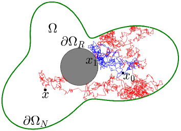
Figure 1: Illustration of a confining domain $\Omega$ with a smooth boundary $\partial\Omega$, which is split into two disjoint parts: a reflecting boundary $\partial\Omega_{N}$ (in green) and a reactive region $\partial\Omega_{R}$ (the frontier of a gray obstacle). A simulated trajectory, started from $\bm{x}_{0}$ and arrived in $\bm{x}$, exhibits multiple failed attempts to react on $\partial\Omega_{R}$ before the successful reaction (binding) at an intermediate point $\bm{x}_{1}$ (path in blue). After staying in the bound state for a random waiting time, the particle was released from $\bm{x}_{1}$ and resumed its bulk diffusion toward the arrival point $\bm{x}$ (path in red).

II.1 Binding events

The encounter-based approach employs the statistics of encounters between the diffusing particle and the reactive region $\partial\Omega_{R}$ to implement surface reactions [106]. As the details of this approach were presented in earlier publications [106, 107, 108, 109, 110], we just sketch the main steps and “ingredients” needed for our computation.

In addition to the (random) position $\bm{X}_{t}$ of the particle at time $t$, we introduce its boundary local time $\ell_{t}$ on $\partial\Omega_{R}$ as

$$\ell_{t}=\lim\limits_{a\to 0}a\,\mathcal{N}_{t}^{(a)},$$ (17)

where $\mathcal{N}_{t}^{(a)}$ is the (random) number of downcrossings of a thin layer of width $a$ near $\partial\Omega_{R}$ up to time $t$. Each such downcrossing can be understood as an encounter between the particle and the substrate $\partial\Omega_{R}$ at a given spatial resolution $a$. As $a\to 0$, $\mathcal{N}_{t}^{(a)}$ diverges due to the self-similar character of Brownian motion but its rescaling by $a$ yields a nontrivial limit $\ell_{t}$, which is a non-decreasing process (with $\ell_{0}=0$) that increments at each encounter of the particle with $\partial\Omega_{R}$ [111, 112, 113]. The boundary local time should not be confused with the local time in a bulk point, which was thoroughly studied (see [114, 115] and references therein). Despite its name, $\ell_{t}$ has units of length. While physical time $t$ is a proxy of the number of particle’s jumps in the bulk, the boundary local time $\ell_{t}$ characterizes the number of jumps onto the surface [107]. In this light, both quantities are complementary and tightly related (see [106] for further discussion). The diffusive dynamics of the particle is fully described by the pair $(\bm{X}_{t},\ell_{t})$, whose probability density is called the full propagator $P(\bm{x},\ell,t|\bm{x}_{0})$. The crucial distinction of the encounter-based approach from conventional methods is that the full propagator characterizes purely diffusive dynamics by treating the region $\partial\Omega_{R}$ as reflecting. In turn, surface reactions on $\partial\Omega_{R}$ are then introduced explicitly via an appropriate stopping condition.

In fact, as discussed earlier, the reaction event is preceded by a sequence of failed reaction attempts at each encounter with $\partial\Omega_{R}$. In other words, the reaction occurs at the first instance $\mathcal{T}$ when the boundary local time (the proxy of the failed attempts) exceeds some threshold $\hat{\ell}$:

$$\mathcal{T}=\inf\{t>0~{}:~{}\ell_{t}>\hat{\ell}\}.$$ (18)

The choice of this threshold selects the mechanism of surface reaction [106]. For instance, if $\hat{\ell}=0$, the reaction occurs when the boundary local time $\ell_{t}$ first exceeds $0$, i.e., when the particle first encounters the region $\partial\Omega_{R}$. This is the perfect reaction introduced by Smoluchowski [1]. In turn, if the particle attempts to react independently on each encounter with probability $\rho\approx a\kappa_{0}/D\ll 1$, the probability of no surface reaction up to the $n$-th encounter is

$$1-\sum\limits_{k=1}^{n}\rho(1-\rho)^{k-1}=(1-\rho)^{n}\approx e^{-\rho n}\approx e^{-q\ell},$$ (19)

where $q=\kappa_{0}/D$, $\ell=na$, and the auxiliary parameter $a$ is a small width of the reactive layer (which is needed here as a sort of regularization but then eliminated in the limit $a\to 0$). By introducing an exponentially distributed random threshold $\hat{\ell}$ such that $\mathbb{P}\{\ell<\hat{\ell}\}=e^{-q\ell}$ and associating the $n$-th reaction attempt to the number of encounters $\mathcal{N}_{t}^{(a)}\approx\ell_{t}/a$ up to time $t$, one sees that the condition $\ell_{t}<\hat{\ell}$ incorporates the survival of the particle in the presence of surface reactions on $\partial\Omega_{R}$ with a constant reactivity $\kappa_{0}$. Most importantly, the encounter-based approach allows one to go far beyond this classical mechanism and to describe much more general and sophisticated surface reactions by means of a random threshold $\hat{\ell}$ obeying a general probability density $\psi(\ell)$, as discussed in this paper.

Let $G_{\psi}(\bm{x},t|\bm{x}_{0})$ denote the generalized propagator in the presence of irreversible forward reaction on $\partial\Omega_{R}$, i.e., $G_{\psi}(\bm{x},t|\bm{x}_{0})$ is the probability density of diffusion from $\bm{x}_{0}$ to $\bm{x}$ in time $t$ under the survival condition (no forward reaction on $\partial\Omega_{R}$ up to time $t$). As the survival condition can be written in terms of the boundary local time, $\ell_{t}<\hat{\ell}$, one gets

$$G_{\psi}(\bm{x},t|\bm{x}_{0})=\int\limits_{0}^{\infty}d\ell\,\Psi(\ell)\,P(\bm{x},\ell,t|\bm{x}_{0}),$$ (20)

where

$$\Psi(\ell)=\mathbb{P}\{\ell<\hat{\ell}\}=\int\limits_{\ell}^{\infty}d\ell^{\prime}\,\psi(\ell^{\prime}).$$ (21)

In other words, the full propagator $P(\bm{x},\ell,t|\bm{x}_{0})$ that treats $\partial\Omega_{R}$ as reflecting, is explicitly complemented by the survival condition $\ell_{t}<\hat{\ell}$, which is fulfilled with probability $\Psi(\ell)$ for a given realized value $\ell$ of the boundary local time $\ell_{t}$. The above integral sums up contributions from all possible realizations of $\ell_{t}$. The associated probability flux density on the reactive region $\partial\Omega_{R}$ reads

$$j_{\psi}(\bm{x},t|\bm{x}_{0})=-D\partial_{n}G_{\psi}(\bm{x},t|\bm{x}_{0})\quad(\bm{x}\in\partial\Omega_{R}).$$ (22)

This quantity characterizes a single binding event (the unbinding mechanism will be introduced in Sec. II.2).

In the case of Markovian binding, Eq. (13) implies $\Psi(\ell)=e^{-q\ell}$, so that one retrieves the conventional propagator

$$G_{q}(\bm{x},t|\bm{x}_{0})=\int\limits_{0}^{\infty}d\ell\,e^{-q\ell}\,P(\bm{x},\ell,t|\bm{x}_{0}),$$ (23)

that satisfies the Robin boundary condition on $\partial\Omega_{R}$ (see [106])

$$-\partial_{n}G_{q}(\bm{x},t|\bm{x}_{0})=q\,G_{q}(\bm{x},t|\bm{x}_{0})\quad(\bm{x}\in\partial\Omega_{R}),$$ (24)

and the corresponding probability flux density

$$j_{q}(\bm{x},t|\bm{x}_{0})=-D\partial_{n}G_{q}(\bm{x},t|\bm{x}_{0})\quad(\bm{x}\in\partial\Omega_{R}).$$ (25)

We will often refer to two particular limits: $q=\infty$ and $q=0$. The quantities $G_{q}(\bm{x},t|\bm{x}_{0})$ and $j_{q}(\bm{x},t|\bm{x}_{0})$ can be represented via spectral expansions over the eigenvalues and eigenfunctions of the Laplace operator [9, 116, 117]. Unfortunately, these commonly used eigenfunctions are not suitable to access the generalized propagator $G_{\psi}(\bm{x},t|\bm{x}_{0})$ that does not satisfy the Robin boundary condition (24).

This problem was solved in [106] by using the Dirichlet-to-Neumann operator $\mathcal{M}_{p}$. This operator acts on an appropriate space of functions on $\partial\Omega_{R}$ as follows: for a function $f$ on $\partial\Omega_{R}$, one finds the solution $u$ of the boundary value problem

$$(p-D\Delta)u =0\quad(\bm{x}\in\Omega),$$ (26a)

$$u =f\quad(\bm{x}\in\partial\Omega_{R}),$$ (26b)

$$\partial_{n}u =0\quad(\bm{x}\in\partial\Omega_{N}),$$ (26c)

evaluates its normal derivative on $\partial\Omega_{R}$, $(\partial_{n}u)|_{\partial\Omega_{R}}$, and associates it to $f$:

$$\mathcal{M}_{p}~{}:~{}f\to(\partial_{n}u)|_{\partial\Omega_{R}}\quad\textrm{or}\quad\mathcal{M}_{p}f=(\partial_{n}u)|_{\partial\Omega_{R}}.$$ (27)

Intuitively, the operator $\mathcal{M}_{p}$ transforms the Dirichlet boundary condition $u=f$ on $\partial\Omega_{R}$ to an equivalent Neumann boundary condition $\partial_{n}u=\mathcal{M}_{p}f$ on $\partial\Omega_{R}$. In physical terms, if $f$ is understood as a density of particles maintained on $\partial\Omega_{R}$, the operator $\mathcal{M}_{p}$ determines their steady-state diffusive flux density $D\mathcal{M}_{p}f=D(\partial_{n}u)|_{\partial\Omega_{R}}$ into the reactive bulk (with a bulk reaction rate $p$). In the particular case $p=0$, a similar problem arises in heat transfer from the boundary $\partial\Omega_{R}$ with an imposed temperature profile $f$, so that $\mathcal{M}_{0}f$ is proportional to the steady-state temperature flux density into the bulk; moreover, the analogy with electrostatics allows one to interpret $f$ as a charge density, for which $\mathcal{M}_{0}f$ determines the current density.

The Dirichlet-to-Neumann operator was thoroughly investigated for the case when $\partial\Omega_{R}=\partial\Omega$ (i.e., $\partial\Omega_{N}=\emptyset$) [118, 119, 120, 121, 122, 123, 124]. We conjecture that the inclusion of the additional boundary condition (26c) on the reflecting part $\partial\Omega_{N}$ does not affect general properties of this operator; in particular, as the region $\partial\Omega_{R}$ is bounded, $\mathcal{M}_{p}$ remains to be self-adjoint pseudo-differential operator with a discrete spectrum for any $p\geq 0$. Its eigenvalues can be enumerated in an ascending order,

$$0\leq\mu_{0}^{(p)}\leq\mu_{1}^{(p)}\leq\ldots\leq\mu_{k}^{(p)}\leq\ldots\nearrow+\infty,$$ (28)

while the eigenfunctions $\{v_{k}^{(p)}\}$ form a complete orthonormal basis in the space $L_{2}(\partial\Omega_{R})$ of square integrable functions on $\partial\Omega_{R}$. While we checked these spectral proprieties numerically for various domains (see an example in Sec. III), a mathematical proof of this extension is beyond the scope of this paper.

The following spectral expansion of the generalized propagator in the Laplace domain was derived in [106]:

$$\tilde{G}_{\psi}(\bm{x},p|\bm{x}_{0}) =\tilde{G}_{\infty}(\bm{x},p|\bm{x}_{0})$$ (29)

$$+\frac{1}{D}\sum\limits_{k=0}^{\infty}[V_{k}^{(p)}(\bm{x}_{0})]^{*}V_{k}^{(p)}(\bm{x})\frac{1-\bar{\psi}(\mu_{k}^{(p)})}{\mu_{k}^{(p)}}\,,$$

where asterisk denotes complex conjugate,

$$\bar{\psi}(\mu)=\int\limits_{0}^{\infty}d\ell\,e^{-\mu\ell}\,\psi(\ell)$$ (30)

is the Laplace transform of $\psi(\ell)$ (we use bar instead of tilde here to highlight different units),

$$V_{k}^{(p)}(\bm{x}_{0})=\int\limits_{\partial\Omega_{R}}d\bm{x}\,\tilde{j}_{\infty}(\bm{x},p|\bm{x}_{0})\,v_{k}^{(p)}(\bm{x}),$$ (31)

and $\tilde{G}_{\infty}(\bm{x},p|\bm{x}_{0})$ and $\tilde{j}_{\infty}(\bm{x},p|\bm{x}_{0})$ are the Laplace transforms of $G_{\infty}(\bm{x},t|\bm{x}_{0})$ and $j_{\infty}(\bm{x},t|\bm{x}_{0})$, respectively.

For the conventional case of a constant reactivity, $\psi(\ell)$ is given by Eq. (13) and thus $\bar{\psi}(\mu)=1/(1+\mu/q)$, so that Eq. (29) is reduced to

$$\tilde{G}_{q}(\bm{x},p|\bm{x}_{0})=\tilde{G}_{\infty}(\bm{x},p|\bm{x}_{0})+\frac{1}{D}\sum\limits_{k=0}^{\infty}\frac{[V_{k}^{(p)}(\bm{x}_{0})]^{*}V_{k}^{(p)}(\bm{x})}{q+\mu_{k}^{(p)}}\,.$$ (32)

Setting $q=0$, one also gets the identity

$$\tilde{G}_{0}(\bm{x},p|\bm{x}_{0})=\tilde{G}_{\infty}(\bm{x},p|\bm{x}_{0})+\sum\limits_{k=0}^{\infty}\frac{[V_{k}^{(p)}(\bm{x}_{0})]^{*}V_{k}^{(p)}(\bm{x})}{D\mu_{k}^{(p)}}\,,$$ (33)

that allows one to write alternative representations

$$\tilde{G}_{q}(\bm{x},p|\bm{x}_{0})=\tilde{G}_{0}(\bm{x},p|\bm{x}_{0})-\frac{1}{D}\sum\limits_{k=0}^{\infty}\frac{[V_{k}^{(p)}(\bm{x}_{0})]^{*}V_{k}^{(p)}(\bm{x})}{\mu_{k}^{(p)}(1+\mu_{k}^{(p)}/q)}$$ (34)

and

$$\tilde{G}_{\psi}(\bm{x},p|\bm{x}_{0}) =\tilde{G}_{0}(\bm{x},p|\bm{x}_{0})$$ (35)

$$-\frac{1}{D}\sum\limits_{k=0}^{\infty}[V_{k}^{(p)}(\bm{x}_{0})]^{*}V_{k}^{(p)}(\bm{x})\frac{\bar{\psi}(\mu_{k}^{(p)})}{\mu_{k}^{(p)}}\,.$$

As a consequence, we find

$$\tilde{j}_{\psi}(\bm{x},p|\bm{x}_{0}) =\left.-D\partial_{n}\tilde{G}_{\psi}(\bm{x},p|\bm{x}_{0})\right|_{\partial\Omega_{R}}$$

$$=\sum\limits_{k=0}^{\infty}[V_{k}^{(p)}(\bm{x}_{0})]^{*}v_{k}^{(p)}(\bm{x})\,\bar{\psi}(\mu_{k}^{(p)})\,,$$ (36)

where we used the property $(\partial_{n}V_{k}^{(p)})|_{\partial\Omega_{R}}=\mu_{k}^{(p)}v_{k}^{(p)}$, given that $v_{k}^{(p)}$ is an eigenfunction of the Dirichlet-to-Neumann operator $\mathcal{M}_{p}$.

In summary, the generalized propagator $G_{\psi}(\bm{x},t|\bm{x}_{0})$ and related quantities fully characterize diffusion-controlled reactions with irreversible binding described by the probability density $\psi(\ell)$. The next step consists in implementing unbinding events.

II.2 Unbinding events

Let us now merge the general mechanism of binding events with a general waiting time distribution for unbinding events. Using the renewal technique, one can compute the propagator $Q(\bm{x},t|\bm{x}_{0})$ of reversible diffusion-controlled reactions as

$$Q(\bm{x},t|\bm{x}_{0})=G_{\psi}(\bm{x},t|\bm{x}_{0})+\int\limits_{\partial\Omega_{R}}d\bm{x}_{1}\int\limits_{0}^{t}dt_{1}\int\limits_{t_{1}}^{t}dt^{\prime}_{1}$$

$$\times j_{\psi}(\bm{x}_{1},t_{1}|\bm{x}_{0})\phi(t^{\prime}_{1}-t_{1})G_{\psi}(\bm{x},t-t^{\prime}_{1}|\bm{x}_{1})+\ldots.$$ (37)

The first term accounts for the random trajectories from $\bm{x}_{0}$ to $\bm{x}$ without any binding, whose fraction is precisely given by $G_{\psi}(\bm{x},t|\bm{x}_{0})$. In the second term, the particle binds at time $t_{1}$ on the point $\bm{x}_{1}\in\partial\Omega_{R}$ (with probability $j_{\psi}(\bm{x}_{1},t_{1}|\bm{x}_{0})d\bm{x}_{1}dt_{1}$), stays in the bound state for the time $t^{\prime}_{1}-t_{1}$ (with probability $\phi(t^{\prime}_{1}-t_{1})dt^{\prime}_{1}$), unbinds and diffuses from $\bm{x}_{1}$ to $\bm{x}$ within the remaining time $t-t^{\prime}_{1}$ (with probability density $G_{\psi}(\bm{x},t-t^{\prime}_{1}|\bm{x}_{1})$). As the binding position and time as well as the duration of the bound state are random, one integrates over all their possible realizations. The next terms in this expression account for two, three, etc. binding events.

With the help of the Laplace transform, one can turn convolutions in time into products, yielding

$$\tilde{Q}(\bm{x},p|\bm{x}_{0}) =\tilde{G}_{\psi}(\bm{x},p|\bm{x}_{0})$$ (38)

$$+\int\limits_{\partial\Omega_{R}}d\bm{x}_{1}\,\tilde{j}_{\psi}(\bm{x}_{1},p|\bm{x}_{0})\tilde{\phi}(p)\tilde{G}_{\psi}(\bm{x},p|\bm{x}_{1})+\ldots.$$

Using the spectral expansions (29, 36), one can evaluate the integrals over the intermediate binding positions $\bm{x}_{1},\bm{x}_{2},\ldots$ in Eq. (38) due to the orthogonality of eigenfunctions $\{v_{k}^{(p)}\}$ and then sum up all contributions as a geometric series to get

$$\tilde{Q}(\bm{x},p|\bm{x}_{0}) =\tilde{G}_{\infty}(\bm{x},p|\bm{x}_{0})+\frac{1}{D}\sum\limits_{k=0}^{\infty}[V_{k}^{(p)}(\bm{x}_{0})]^{*}V_{k}^{(p)}(\bm{x})$$

$$\times\frac{1-\bar{\psi}(\mu_{k}^{(p)})}{\mu_{k}^{(p)}[1-\tilde{\phi}(p)\bar{\psi}(\mu_{k}^{(p)})]}\,.$$ (39)

Using the identity (33), one can rewrite Eq. (39) as

$$\tilde{Q}(\bm{x},p|\bm{x}_{0}) =\tilde{G}_{0}(\bm{x},p|\bm{x}_{0})-\frac{1}{D}\sum\limits_{k=0}^{\infty}[V_{k}^{(p)}(\bm{x}_{0})]^{*}V_{k}^{(p)}(\bm{x})$$

$$\times\frac{(1-\tilde{\phi}(p))\,\bar{\psi}(\mu_{k}^{(p)})}{\mu_{k}^{(p)}[1-\tilde{\phi}(p)\bar{\psi}(\mu_{k}^{(p)})]}\,.$$ (40)

This spectral expansion is one of the main general results of the paper. It shows how the geometric structure of the confining domain $\Omega$, expressed in terms of the spectral quantities $\mu_{k}^{(p)}$ and $V_{k}^{(p)}(\bm{x})$, is coupled to the binding and unbinding kinetics expressed in terms of $\bar{\psi}(\mu)$ and $\tilde{\phi}(p)$, respectively. This expansion holds for any $p\geq 0$ and any confining domain $\Omega$ with a smooth boundary $\partial\Omega$ and a bounded region $\partial\Omega_{R}$.

In the same way, one can also compute the propagator $Q_{b}(\bm{x},t|\bm{x}_{0})$ to be in the bound state at $\bm{x}\in\partial\Omega_{R}$ at time $t$. The renewal technique yields

$$Q_{b}(\bm{x},t|\bm{x}_{0})=\int\limits_{0}^{t}dt^{\prime}\,j_{\psi}(\bm{x},t^{\prime}|\bm{x}_{0})\,\Phi(t-t^{\prime})$$

$$+\int\limits_{\partial\Omega_{R}}d\bm{x}_{1}\int\limits_{0}^{t}dt_{1}\int\limits_{t_{1}}^{t}dt^{\prime}_{1}\int\limits_{t^{\prime}_{1}}^{t}dt^{\prime}\,j_{\psi}(\bm{x},t_{1}|\bm{x}_{0})\,\phi(t^{\prime}_{1}-t_{1})$$

$$\times j_{\psi}(\bm{x},t^{\prime}-t^{\prime}_{1}|\bm{x}_{1})\Phi(t-t^{\prime})+\ldots,$$

where $\Phi(t)=\int\nolimits_{t}^{\infty}dt^{\prime}\,\phi(t^{\prime})$ is the probability of no desorption up to time $t$. The first term describes the first binding at $\bm{x}$ at time $t^{\prime}$ and staying there until $t$, while the second and other terms account for multiple unbinding-rebinding events. Applying the Laplace transform and using the spectral expansions, we get

$$\tilde{Q}_{b}(\bm{x},p|\bm{x}_{0})=\sum\limits_{k=0}^{\infty}[V_{k}^{(p)}(\bm{x}_{0})]^{*}\,v_{k}(\bm{x})\frac{(1-\tilde{\phi}(p))\bar{\psi}(\mu_{k}^{(p)})}{p[1-\tilde{\phi}(p)\bar{\psi}(\mu_{k}^{(p)})]}\,,$$ (41)

where we used that $\tilde{\Phi}(p)=(1-\tilde{\phi}(p))/p$. Evaluating the normal derivative of the propagator $\tilde{Q}(\bm{x},p|\bm{x}_{0})$ from Eq. (40) on $\partial\Omega_{R}$, we deduce

$$p\,\tilde{Q}_{b}(\bm{x},p|\bm{x}_{0})=-D\partial_{n}\tilde{Q}(\bm{x},p|\bm{x}_{0})\quad(\bm{x}\in\partial\Omega_{R})$$ (42)

that reads in time domain as

$$\partial_{t}Q_{b}(\bm{x},t|\bm{x}_{0})=-D\partial_{n}Q(\bm{x},t|\bm{x}_{0})\quad(\bm{x}\in\partial\Omega_{R}).$$ (43)

In other words, the back-reaction boundary condition (6) remains valid in the general case of non-Markovian binding/unbinding kinetics. In turn, Eq. (5) representing the first-order kinetics, is only retrieved when both $\psi(\ell)$ and $\phi(t)$ are exponential (see Sec. II.3).

Note that if the particle was initially in the bound state (at a boundary point $\bm{x}_{0}\in\partial\Omega_{R}$), one has to include an additional waiting step until its first desorption. As a consequence, the Laplace transform of the associated propagator that we denote $Q(\bm{x},t|\bm{x}_{0},b)$ is

$$\tilde{Q}(\bm{x},p|\bm{x}_{0},b)=\tilde{\phi}(p)\tilde{Q}(\bm{x},p|\bm{x}_{0})$$ (44)

$$=\frac{1}{D}\sum\limits_{k=0}^{\infty}[V_{k}^{(p)}(\bm{x}_{0})]^{*}V_{k}^{(p)}(\bm{x})\frac{(1-\bar{\psi}(\mu_{k}^{(p)}))\,\tilde{\phi}(p)}{\mu_{k}^{(p)}[1-\tilde{\phi}(p)\bar{\psi}(\mu_{k}^{(p)})]}\,,$$

where we used Eq. (39).

The integral of Eq. (40) over $\bm{x}\in\Omega$ determines the Laplace transform of the probability $S(t|\bm{x}_{0})$ that the particle is unbound at time $t$:

$$\tilde{S}(p|\bm{x}_{0})=\int\limits_{\Omega}d\bm{x}\,\tilde{Q}(\bm{x},p|\bm{x}_{0})=\frac{1}{p}$$ (45)

$$-\sum\limits_{k=0}^{\infty}[V_{k}^{(p)}(\bm{x}_{0})]^{*}\frac{\bar{\psi}(\mu_{k}^{(p)})(1-\tilde{\phi}(p))}{p[1-\tilde{\phi}(p)\bar{\psi}(\mu_{k}^{(p)})]}\int\limits_{\partial\Omega_{R}}d\bm{x}\,v_{k}^{(p)}(\bm{x}),$$

where we used the following identity from [125]

$$\int\limits_{\Omega}d\bm{x}\,V_{k}^{(p)}(\bm{x})=\frac{D}{p}\mu_{k}^{(p)}\int\limits_{\partial\Omega_{R}}d\bm{x}\,v_{k}^{(p)}(\bm{x}).$$ (46)

If there was a uniform concentration $c_{0}$ of particles at time $0$, their concentration $c(\bm{x},t)$ at time $t$ is given by Eq. (15). According to Eq. (40), the propagator is symmetric with respect to the exchange of $\bm{x}$ and $\bm{x}_{0}$, $Q(\bm{x},t|\bm{x}_{0})=Q(\bm{x}_{0},t|\bm{x})$, so that

$$c(\bm{x},t)=\int\limits_{\Omega}d\bm{x}_{0}\,c_{0}\,Q(\bm{x},t|\bm{x}_{0})=c_{0}\,S(t|\bm{x}),$$ (47)

and the latter is given by Eq. (45) in the Laplace domain. The diffusive flux of particles on the reactive region is then given in the Laplace domain as

$$\tilde{J}(p) =\int\limits_{\partial\Omega_{R}}d\bm{x}\,\bigl{(}-D\partial_{n}\tilde{c}(\bm{x},p)\bigr{)}$$ (48)

$$=c_{0}D\sum\limits_{k=0}^{\infty}\frac{\mu_{k}^{(p)}\bar{\psi}(\mu_{k}^{(p)})(1-\tilde{\phi}(p))}{p[1-\tilde{\phi}(p)\bar{\psi}(\mu_{k}^{(p)})]}\left|\int\limits_{\partial\Omega_{R}}d\bm{x}\,v_{k}^{(p)}(\bm{x})\right|^{2}.$$

In summary, we developed a general mathematical formalism to describe a very broad class of reversible diffusion-controlled reactions. At a microscopic level, one can think of a particle diffusing inside a confining domain $\Omega$ toward a reactive region $\partial\Omega_{R}$. When the particle approached $\partial\Omega_{R}$ close enough, a local short-range interaction attempts to bind it (e.g., due to attractive electrostatic potential, formation of covalent or ionic bonds, mutual affinity, conformational change, local minimum of a potential energy, entropic barrier, adsorption, transfer through a channel, etc.). If the binding attempt fails, the particle continues its bulk diffusion until the next encounter with $\partial\Omega_{R}$, and so on. The random number of failed attempts until the successful binding is represented by the threshold $\hat{\ell}$ drawn from the probability density $\psi(\ell)$ that characterizes binding kinetics. After staying in the bound state for a random waiting time $\hat{t}$ drawn from the probability density $\phi(t)$ that characterizes unbinding kinetics, the particle is released into the bulk to resume its diffusion. As the binding event is preceded by multiple diffusive excursions in the bulk, the generating function $\bar{\psi}(\mu)=\int\nolimits_{0}^{\infty}d\ell\,e^{-\mu\ell}\psi(\ell)$ of the random threshold $\hat{\ell}$ is tightly coupled to the geometric structure of the confining domain $\Omega$ that are captured via the eigenmodes of the Dirichlet-to-Neumann operator. In turn, the unbinding event is simply a halt at the binding point for a random waiting time, which is described by $\phi(t)$ or $\tilde{\phi}(p)=\int\nolimits_{0}^{\infty}dt\,e^{-pt}\phi(t)$, independently of the confinement. For more sophisticated unbinding events (such as, e.g., surface diffusion), $\tilde{\phi}(p)$ is expected to become coupled to the geometric structure of the reactive region $\partial\Omega_{R}$. In this way, one can potentially retrieve and further generalize the description of intermittent diffusions [126], in particular, those with alternating tours of bulk and surface diffusion [127, 128, 129, 130, 131, 132, 133, 134, 135, 136]. However, such an extension is beyond the scope of this paper.

II.3 Markovian binding kinetics

Let us first inspect the Markovian binding kinetics determined by the exponential distribution in Eq. (13). In this case, Eq. (40) reads

$$\tilde{Q}(\bm{x},p|\bm{x}_{0})=\tilde{G}_{0}(\bm{x},p|\bm{x}_{0})-\frac{1}{D}\sum\limits_{k=0}^{\infty}\frac{[V_{k}^{(p)}(\bm{x}_{0})]^{*}V_{k}^{(p)}(\bm{x})}{\mu_{k}^{(p)}(1+\mu_{k}^{(p)}/q_{p})}\,,$$ (49)

with

$$q_{p}=q(1-\tilde{\phi}(p))=\tilde{\kappa}(p)/D\,,$$ (50)

or, equivalently,

$$\tilde{Q}(\bm{x},p|\bm{x}_{0})=\tilde{G}_{\infty}(\bm{x},p|\bm{x}_{0})+\frac{1}{D}\sum\limits_{k=0}^{\infty}\frac{[V_{k}^{(p)}(\bm{x}_{0})]^{*}V_{k}^{(p)}(\bm{x})}{\mu_{k}^{(p)}+q_{p}}\,.$$ (51)

In line with the former description of reversible reactions in Sec. I, we retrieved the spectral expansion (34), in which the constant reactivity parameter $q$ is replaced by the $p$-dependent function $q_{p}$ from Eq. (50). In other words, the propagator $\tilde{Q}(\bm{x},p|\bm{x}_{0})$ satisfies the Robin boundary condition

$$-D\partial_{n}\tilde{Q}(\bm{x},p|\bm{x}_{0})=\tilde{\kappa}(p)\tilde{Q}(\bm{x},p|\bm{x}_{0})\quad(\bm{x}\in\partial\Omega_{R}),$$ (52)

with $\tilde{\kappa}(p)=q_{p}D$ (see Sec. II.4 for further discussions). One also sees that the results for irreversible binding are retrieved by formally setting $\tilde{\phi}(p)\equiv 0$.

The inverse Laplace transform of Eq. (52) yields a convolution-type boundary condition on $\partial\Omega_{R}$:

$$-D\partial_{n}Q(\bm{x},t|\bm{x}_{0})=\int\limits_{0}^{t}dt^{\prime}\,\mathcal{K}(t-t^{\prime})\,Q(\bm{x},t^{\prime}|\bm{x}_{0}),$$ (53)

with

$$\mathcal{K}(t)=\kappa_{0}\bigl{(}\delta(t)-\phi(t)\bigr{)},\quad\kappa_{0}=qD.$$ (54)

This is a generalization of Eqs. (10, 11). This is also an extension of the results by Agmon and Weiss [86] to arbitrary confining domains. Whatever the distribution of waiting times is, the memory kernel induces a sort of delayed feedback from the particles that are “stored” in the bound state and progressively released at later times. We inspect the consequences of these memory effects for general binding/unbinding kinetics in Sec. II.5.

II.4 Robin boundary condition

Let us return to the general setting. It is easy to check that the Laplace-transformed propagator $\tilde{Q}(\bm{x},p|\bm{x}_{0})$ given by Eq. (40) satisfies the modified Helmholtz equation, as the conventional propagators do:

$$(p-D\Delta)\tilde{Q}(\bm{x},p|\bm{x}_{0})=\delta(\bm{x}-\bm{x}_{0})\quad(\bm{x}\in\Omega),$$ (55)

where $\delta(\bm{x}-\bm{x}_{0})$ is the Dirac distribution. Expectedly, its inverse Laplace transform yields the diffusion equation in time domain,

$$\partial_{t}Q(\bm{x},t|\bm{x}_{0})=D\Delta Q(\bm{x},t|\bm{x}_{0})\quad(\bm{x}\in\Omega),$$ (56)

with the standard initial condition $Q(\bm{x},0|\bm{x}_{0})=\delta(\bm{x}-\bm{x}_{0})$ that affirms that $\bm{x}_{0}$ is the starting point at time $0$. As there is no surface reaction on the reflecting boundary $\partial\Omega_{N}$, the Neumann boundary condition applies:

$$\partial_{n}\tilde{Q}(\bm{x},p|\bm{x}_{0})=0\quad(\bm{x}\in\partial\Omega_{N})$$ (57)

(and the same holds in the time domain). Let us now inspect the boundary condition on the reactive part $\partial\Omega_{R}$.

As we discussed earlier, the Markovian binding kinetics is tightly related to the Robin boundary condition for the Laplace-transformed propagator $\tilde{Q}(\bm{x},p|\bm{x}_{0})$. However, this boundary condition does not hold in general for non-Markovian binding. Using Eqs. (39, 40), one can easily check that

$$\left.-D\partial_{n}\tilde{Q}(\bm{x},p|\bm{x}_{0})\right|_{\bm{x}\in\partial\Omega_{R}} =\sum\limits_{k=0}^{\infty}[V_{k}^{(p)}(\bm{x}_{0})]^{*}V_{k}^{(p)}(\bm{x})$$

$$\times\frac{\bar{\psi}(\mu_{k}^{(p)})(1-\tilde{\phi}(p))}{1-\tilde{\phi}(p)\bar{\psi}(\mu_{k}^{(p)})}\,,$$

$$\left.D\tilde{Q}(\bm{x},p|\bm{x}_{0})\right|_{\bm{x}\in\partial\Omega_{R}} =\sum\limits_{k=0}^{\infty}[V_{k}^{(p)}(\bm{x}_{0})]^{*}V_{k}^{(p)}(\bm{x})$$

$$\times\frac{1-\bar{\psi}(\mu_{k}^{(p)})}{\mu_{k}^{(p)}[1-\tilde{\phi}(p)\bar{\psi}(\mu_{k}^{(p)})]}\,.$$

These two functions can satisfy the Robin boundary condition (52) only if each term in one series is proportional to the corresponding term in the other, i.e., if

$$\frac{\bar{\psi}(\mu_{k}^{(p)})(1-\tilde{\phi}(p))}{1-\tilde{\phi}(p)\bar{\psi}(\mu_{k}^{(p)})}=q_{p}\frac{1-\bar{\psi}(\mu_{k}^{(p)})}{\mu_{k}^{(p)}[1-\tilde{\phi}(p)\bar{\psi}(\mu_{k}^{(p)})]}$$

for some proportionality coefficient $q_{p}$, from which

$$q_{p}=(1-\tilde{\phi}(p))\frac{\mu_{k}^{(p)}\bar{\psi}(\mu_{k}^{(p)})}{1-\bar{\psi}(\mu_{k}^{(p)})}\,.$$ (58)

As the left-hand side does not depend on $k$, the right-hand side should not as well, i.e., one should have

$$\frac{\mu_{k}^{(p)}\bar{\psi}(\mu_{k}^{(p)})}{1-\bar{\psi}(\mu_{k}^{(p)})}=q$$

for some constant $q$, and thus $\bar{\psi}(\mu_{k}^{(p)})=1/(1+\mu_{k}^{(p)}/q)$, i.e., the random threshold should obey an exponential distribution with the rate $q$. In other words, if the distribution of $\hat{\ell}$ is exponential, the propagator $\tilde{Q}(\bm{x},p|\bm{x}_{0})$ satisfies the Robing boundary condition (52). In turn, any non-exponential density $\psi(\ell)$ would in general invalidate the Robin boundary condition.

Despite this general statement, the Robin boundary condition can still re-appear in some situations. For instance, let us look at the concentration $c(\bm{x},t)$ with the uniform initial condition $c_{0}(\bm{x}_{0})=c_{0}$, which is proportional to $S(t|\bm{x})$ according to Eq. (47). In some symmetric domains, the integral over $\bm{x}\in\partial\Omega_{R}$ may cancel all contributions in Eq. (45) except for $k=0$. In this specific case, $\tilde{c}(\bm{x},p)$ would satisfy the Robin boundary condition

$$-\partial_{n}\tilde{c}(\bm{x},p)=q_{p}\,\tilde{c}(\bm{x},p)\quad(\bm{x}\in\partial\Omega_{R}),$$ (59)

with $q_{p}$ given by Eq. (58) for $k=0$. Indeed, if both $\tilde{c}(\bm{x},p)$ and $\partial_{n}\tilde{c}(\bm{x},p)$ (restricted on $\partial\Omega_{R}$) are determined by a single eigenmode, they are necessarily proportional to each other. In Sec. III, we discuss an explicit example of a spherical target, whose rotational symmetry leads to this situation.

The inverse Laplace transform of Eq. (59) yields again a convolution-type Robin boundary condition (10) in time domain, with the memory kernel $\mathcal{K}(t)$ obtained by the inverse Laplace transform of $\tilde{\kappa}(p)=q_{p}D$:

$$\mathcal{K}(t)=\mathcal{L}^{-1}\left\{D(1-\tilde{\phi}(p))\frac{\mu_{0}^{(p)}\bar{\psi}(\mu_{0}^{(p)})}{1-\bar{\psi}(\mu_{0}^{(p)})}\right\}.$$ (60)

In this case, the statistics of both binding and unbinding events, incorporated through $\bar{\psi}(\mu_{0}^{(p)})$ and $\tilde{\phi}(p)$, as well as the geometric structure of the domain, represented by $\mu_{0}^{(p)}$, all determine the memory kernel. This point was first mentioned in [106]. Moreover, Bressloff showed for simple one-dimensional settings that such memory kernels can be heavy-tailed [109, 137, 138]. We return to this point in Sec. III for the case of a spherical reactive region.

II.5 Long-time behavior

To conclude this section, we investigate the long-time behavior of the propagator $Q(\bm{x},t|\bm{x}_{0})$. We consider general asymptotic expressions

$$\bar{\psi}(\mu) \approx 1-\mu^{\alpha}\ell_{0}^{\alpha}+\ldots\quad(\mu\to 0),$$ (61)

$$\tilde{\phi}(p) \approx 1-p^{\beta}t_{d}^{\beta}+\ldots\quad(p\to 0),$$ (62)

with some exponents $0<\alpha\leq 1$ and $0<\beta\leq 1$ and length and time scales $\ell_{0}$ and $t_{d}$ that characterize binding and unbinding events, respectively. When $\beta=1$, the mean waiting time is finite and equal to $t_{d}$. Similarly, when $\alpha=1$, the mean threshold is finite and equal to $\ell_{0}$. Using the asymptotic expansion [139]

$$\mu_{0}^{(p)}\approx\frac{|\Omega|}{D|\partial\Omega_{R}|}p+\ldots\quad(p\to 0),$$ (63)

where $|\Omega|$ is the volume of $\Omega$, we can write

$$\bar{\psi}(\mu_{0}^{(p)})\approx 1-p^{\alpha}t_{a}^{\alpha}+\ldots\quad(p\to 0),$$ (64)

where

$$t_{a}=\frac{\ell_{0}|\Omega|}{D|\partial\Omega_{R}|}$$ (65)

is a time scale associated to binding events (see Appendix B). Finally, we note that $v_{0}^{(0)}=1/\sqrt{|\partial\Omega_{R}|}$ and thus

$$V_{0}^{(0)}(\bm{x}_{0})=\int\limits_{\partial\Omega_{R}}d\bm{x}\,\tilde{j}_{\infty}(\bm{x},0|\bm{x}_{0})v_{0}^{(0)}(\bm{x})=\frac{1}{\sqrt{|\partial\Omega_{R}|}}$$ (66)

due to the normalization of the probability flux density $j_{\infty}(\bm{x},t|\bm{x}_{0})$.

The first term in Eq. (40) behaves as $\tilde{G}_{0}(\bm{x},p|\bm{x}_{0})\approx 1/(p|\Omega|)$ in the limit $p\to 0$, ensuring that the conventional propagator $G_{0}(\bm{x},t|\bm{x}_{0})$ approaches the uniform distribution in the bounded domain $\Omega$ with reflecting boundary $\partial\Omega$:

$$G_{0}(\bm{x},t|\bm{x}_{0})\approx\frac{1}{|\Omega|}+O(exp)\quad(t\to\infty),$$ (67)

where $O(exp)$ denotes an exponentially decaying correction. In the second term of Eq. (40), let us denote the contributions as

$$\tilde{Q}_{k}(p)=\frac{1}{D}[V_{k}^{(p)}(\bm{x}_{0})]^{*}V_{k}^{(p)}(\bm{x})\frac{\bar{\psi}(\mu_{k}^{(p)})(1-\tilde{\phi}(p))}{\mu_{k}^{(p)}[1-\tilde{\phi}(p)\bar{\psi}(\mu_{k}^{(p)})]}\,.$$ (68)

For the ground eigenmode $k=0$, the substitution of the above small-$p$ expansions yields

$$\tilde{Q}_{0}(p)\approx\frac{p^{\beta-1}t_{d}^{\beta}}{|\Omega|\bigl{(}p^{\alpha}t_{a}^{\alpha}+p^{\beta}t_{d}^{\beta}\bigr{)}}\quad(p\to 0).$$ (69)

Expectedly, it does not depend on the starting point $\bm{x}_{0}$, nor on the arrival point $\bm{x}$. In turn, for other eigenmodes with $k>0$, one has $\mu_{k}^{(p)}\to\mu_{k}^{(0)}>0$ as $p\to 0$ and therefore

$$\tilde{Q}_{k}(p)\approx\frac{[V_{k}^{(0)}(\bm{x}_{0})]^{*}V_{k}^{(0)}(\bm{x})t_{d}^{\beta}\bar{\psi}(\mu_{k}^{(0)})}{D\mu_{k}^{(0)}\bigl{(}1-\bar{\psi}(\mu_{k}^{(0)})\bigr{)}}p^{\beta}\quad(p\to 0).$$ (70)

For any combination of the exponents $\alpha$ and $\beta$, the inverse Laplace transform of this term yields a subleading contribution as compared to $Q_{0}(t)$. As a consequence, we focus on the leading-order term $Q_{0}(t)$.

We distinguish four regimes.

(i) If $\alpha=\beta=1$, one has in the leading order

$$\tilde{Q}_{0}(p)\approx\frac{t_{d}}{|\Omega|(t_{d}+t_{a})p}\quad(p\to 0),$$ (71)

so that

$$Q(\bm{x},t|\bm{x}_{0})\approx\frac{1}{|\Omega|(1+t_{d}/t_{a})}+O(exp)\quad(t\to\infty).$$ (72)

Expectedly, when both binding and unbinding events are characterized by finite means, the system evolves toward an equilibrium distribution, which is uniform inside the confining domain. The probability to be in the unbound state is $1/(1+t_{d}/t_{a})$. An exponential relaxation to the equilibrium is the reminiscent feature of restricted diffusion in a bounded confining domain. It is drastically different from diffusion in unbounded domains, for which the particle can diffuse arbitrarily far away from the reactive region so that the duration of each bulk exploration between consecutive bindings can be very long; in particular, the survival probability for irreversible reactions and the probability to be in the bound state for reversible reactions are known to exhibit power-law decays in time [9, 83, 86, 140, 141, 142, 143].

(ii) If $\alpha<\beta\leq 1$, one has in the leading order

$$\tilde{Q}_{0}(p)\approx\frac{t_{d}^{\beta}}{|\Omega|t_{a}^{\alpha}}p^{-(1+\alpha-\beta)}\quad(p\to 0),$$ (73)

so that

$$Q(\bm{x},t|\bm{x}_{0})\approx\frac{1}{|\Omega|}\biggl{(}1-\frac{t_{d}^{\beta}\,t^{\alpha-\beta}}{t_{a}^{\alpha}\Gamma(1+\alpha-\beta)}\biggr{)}\quad(t\to\infty).$$ (74)

As the binding events are characterized by the smaller exponent $\alpha$, unbinding events more probable at long times. As a consequence, the particle is asymptotically unbound but the approach to this regime is controlled by a slow power-law decay, with the exponent $\alpha-\beta$ (much faster decaying exponential corrections are not relevant here and thus omitted).

(iii) If $\beta<\alpha\leq 1$, one has in the leading order

$$\tilde{Q}_{0}(p)\approx\frac{1}{|\Omega|p}\biggl{(}1-\frac{t_{a}^{\alpha}}{t_{d}^{\beta}}p^{\alpha-\beta}\biggr{)}\quad(p\to 0),$$ (75)

so that

$$Q(\bm{x},t|\bm{x}_{0})\approx\frac{t_{a}^{\alpha}\,t^{\beta-\alpha}}{|\Omega|t_{d}^{\beta}\Gamma(1+\beta-\alpha)}\quad(t\to\infty).$$ (76)

In this case, binding events are characterized by the larger exponent $\alpha$ and thus more probable than the unbinding events so that the particle tends to be asymptotically in the bound state. In particular, the probability to be in the unbound state slowly vanishes as $t^{\beta-\alpha}$, with the exponent $\beta-\alpha$.

(iv) If $\alpha=\beta<1$, we have

$$\tilde{Q}_{0}(p)\approx\frac{1}{|\Omega|p(1+(t_{a}/t_{d})^{\alpha})}\biggl{(}1-\frac{t_{a}^{2\alpha}\,p^{\alpha}}{t_{a}^{\alpha}+t_{d}^{\alpha}}\biggr{)}\quad(p\to 0),$$ (77)

so that

$$Q(\bm{x},t|\bm{x}_{0}) \approx\frac{1}{|\Omega|(1+(t_{d}/t_{a})^{\alpha})}$$ (78)

$$\times\biggl{(}1+\frac{t_{d}^{\alpha}\,t^{-\alpha}}{(1+(t_{d}/t_{a})^{\alpha})\Gamma(1-\alpha)}\biggr{)}\quad(t\to\infty).$$

In this subtle setting, the occurrence of binding and unbinding events is equally rare at long times so that the system approaches an equilibrium uniform distribution, but this power-law approach is much slower than in the case $\alpha=\beta=1$. The asymptotic probability of the unbound state is $1/(1+(t_{d}/t_{a})^{\alpha})$.

The integral over $\bm{x}\in\Omega$ of the above relations removes the factor $1/|\Omega|$ and yields the long-time asymptotic behavior of the probability $S(t|\bm{x}_{0})$, while its multiplication by $c_{0}$ determines the asymptotic behavior of the concentration $c(\bm{x},t)$.

III Spherical target

To illustrate the above general results, we consider restricted diffusion between two concentric spheres of radii $R$ and $L$: $\Omega=\{\bm{x}\in\mathbb{R}^{3}~{}:~{}R<|\bm{x}|<L\}$. The inner sphere represents the reactive region $\partial\Omega_{R}$, while the outer sphere is the reflecting boundary $\partial\Omega_{N}$. This emblematic model for diffusion-controlled reactions was thoroughly investigated (see [40, 101] and references therein). In a similar way, one can obtain the exact results for restricted diffusion on an interval, a half-line, a circular annulus, and the exterior of the cylinder (see [107] and Appendix C). For the sake of clarity, we focus on the probability $S(t|\bm{x}_{0})$ (or, equivalently, on the concentration $c(\bm{x},t)$) and on the diffusive flux $J(t)$.

The eigenbasis of the Dirichlet-to-Neumann operator in this domain is known [107]. In fact, the eigenfunctions $v_{k}^{(p)}$ are given by the normalized spherical harmonics so that the integral over $\partial\Omega_{R}$ in Eq. (45) cancels all terms except the ground eigenmode, for which $v_{0}^{(p)}(\bm{x})=1/\sqrt{|\partial\Omega_{R}|}$. We get then

$$\tilde{S}(p|\bm{x}_{0})=\frac{1}{p}-g_{0}^{(p)}(r_{0})\frac{\bar{\psi}(\mu_{0}^{(p)})(1-\tilde{\phi}(p))}{p[1-\tilde{\phi}(p)\bar{\psi}(\mu_{0}^{(p)})]}\,,$$ (79)

where $r_{0}=|\bm{x}_{0}|$,

$$g_{0}^{(p)}(r) =\frac{R}{r}\,\frac{w(L\sqrt{p/D},r\sqrt{p/D})}{w(L\sqrt{p/D},R\sqrt{p/D})}\,,$$ (80a)

$$w(x,y) =\sinh(x-y)-x\cosh(x-y),$$ (80b)

and

$$\mu_{0}^{(p)}=\frac{1}{R}+\sqrt{p/D}\,\frac{L\sqrt{p/D}\tanh((L-R)\sqrt{p/D})-1}{L\sqrt{p/D}-\tanh((L-R)\sqrt{p/D})}\,.$$ (81)

The diffusive flux (48) reads in the Laplace domain:

$$\tilde{J}(p)=4\pi R^{2}c_{0}D\frac{\mu_{0}^{(p)}(1-\tilde{\phi}(p))\bar{\psi}(\mu_{0}^{(p)})}{p[1-\tilde{\phi}(p)\bar{\psi}(\mu_{0}^{(p)})]}\,.$$ (82)

If the particle was initially in the bound state, the inclusion of an additional waiting step yields

$$\tilde{S}(p|b)=\tilde{\phi}(p)\,\tilde{S}(p|\bm{x}_{0})|_{\partial\Omega_{R}}=\frac{\tilde{\phi}(p)(1-\bar{\psi}(\mu_{0}^{(p)}))}{p[1-\tilde{\phi}(p)\bar{\psi}(\mu_{0}^{(p)})]}\,,$$ (83)

which is independent of the starting point $\bm{x}_{0}$ due to the rotational invariance of the domain.

For Markovian binding kinetics with $\psi(\ell)$ from Eq. (13), one has $\bar{\psi}(\mu)=1/(1+\mu/q)$, so that the above expressions are reduced to

$$\tilde{S}(p|\bm{x}_{0})=\frac{1}{p}-\frac{g_{0}^{(p)}(r_{0})[1-\tilde{\phi}(p)]}{p[1-\tilde{\phi}(p)+\mu_{0}^{(p)}/q]}\,,$$ (84)

$$\tilde{S}(p|b)=\frac{\tilde{\phi}(p)}{p[1+q(1-\tilde{\phi}(p))/\mu_{0}^{(p)}]}\,,$$ (85)

and

$$\tilde{J}(p)=4\pi R^{2}c_{0}D\frac{\mu_{0}^{(p)}(1-\tilde{\phi}(p))}{p(1-\tilde{\phi}(p)+\mu_{0}^{(p)}/q)}\,.$$ (86)

To show the behavior of these quantities in time domain, we will compute their inverse Laplace transforms numerically by using the Talbot algorithm [144].

III.1 Mittag-Leffler model

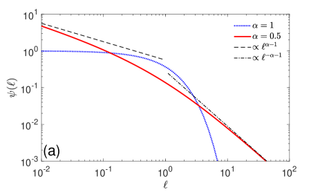
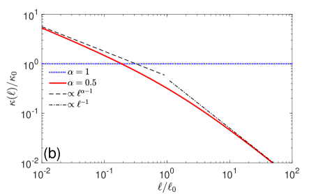
Figure 2: (a) The Mittag-Leffler probability density $\psi(\ell)$ from Eq. (87), with $\ell_{0}=1$ and two exponents: $\alpha=1$ and $\alpha=0.5$. Thin lines indicate the asymptotic relations (90). (b) The associated encounter-dependent reactivity $\kappa(\ell)$ given by Eq. (108). Thin lines indicate the asymptotic relations (109).

In order to illustrate various features of non-Markovian binding/unbinding kinetics, we introduce the Mittag-Leffler model, in which both binding and unbinding events are characterized by Mittag-Leffler distributions:

$$\psi(\ell)=-E_{\alpha,0}(-(\ell/\ell_{0})^{\alpha})/\ell$$ (87)

for the threshold $\hat{\ell}$ determining each binding event, and

$$\phi(t)=-E_{\beta,0}(-(t/t_{d})^{\beta})/t$$ (88)

for the waiting time $\hat{t}$ in each bound state, where

$$E_{\gamma,\delta}(z)=\sum\limits_{k=0}^{\infty}\frac{z^{k}}{\Gamma(\gamma k+\delta)}$$ (89)

is the Mittag-Leffler function. The associated generating functions are particularly simple: $\bar{\psi}(\mu)=1/(1+(\mu\ell_{0})^{\alpha})$ and $\tilde{\phi}(p)=1/(1+(pt_{d})^{\beta})$. Since $E_{1,0}(z)=ze^{z}$, the above distributions become exponential (with $q=1/\ell_{0}$ and $k_{\rm off}=1/t_{d}$) when $\alpha=1$ or $\beta=1$. When the exponent is smaller than $1$, the probability density exhibits a power-law behavior in both limits, e.g.,

$$\psi(\ell) \approx\frac{\ell^{\alpha-1}}{\ell_{0}^{\alpha}\Gamma(\alpha)}\quad(\ell\to 0),$$ (90a)

$$\psi(\ell) \approx\frac{\ell_{0}^{\alpha}\,\ell^{-\alpha-1}}{|\Gamma(-\alpha)|}\quad(\ell\to\infty).$$ (90b)

Note that if $\alpha$ or $\beta$ is equal to $1/2$, the above Mittag-Leffler function can be expressed in terms of the error function $\mathrm{erf}(z)$, e.g., one has for $\alpha=1/2$

$$\psi(\ell)=\frac{1}{\sqrt{\pi\ell_{0}\ell}}-\frac{1}{\ell_{0}}\,\mathrm{erfcx}(\sqrt{\ell/\ell_{0}}),$$ (91)

where $\mathrm{erfcx}(z)=e^{z^{2}}(1-\mathrm{erf}(z))$ is the scaled complementary error function (see Fig. 2(a)).

III.2 Diffusion toward a sphere in $\mathbb{R}^{3}$

Before dwelling on restricted diffusion in the bounded spherical domain, it is instructive to have a look at the limit $L\to\infty$ when the outer reflecting boundary is moved away. This limit corresponds to the most well-studied setting of a particle diffusing in $\mathbb{R}^{3}$ toward a reactive sphere of radius $R$. This is the problem that was addressed in the seminal works by Smoluchowski, Collins and Kimball and many others. Even though we focused on bounded domains in Sec. II, the derived spectral expansions generally remain valid for unbounded domains as well, provided that the reactive region $\partial\Omega_{R}$ is bounded. While the mathematical treatment of general unbounded domains goes beyond the scope of the paper, taking the limit $L\to\infty$ in the considered example of concentric spheres is straightforward. For instance, one gets immediately

$$\tilde{S}(p|\bm{x}_{0}) =\frac{1}{p}-\frac{R}{r_{0}}e^{-(r_{0}-R)\sqrt{p/D}}$$

$$\times\frac{(1-\tilde{\phi}(p))\bar{\psi}(1/R+\sqrt{p/D})}{p[1-\tilde{\phi}(p)\bar{\psi}(1/R+\sqrt{p/D})]}$$ (92)

and

$$\tilde{S}(p|b)=\frac{\tilde{\phi}(p)(1-\bar{\psi}(1/R+\sqrt{p/D}))}{p[1-\tilde{\phi}(p)\bar{\psi}(1/R+\sqrt{p/D})]}\,.$$ (93)

For the Markovian binding, these expressions are reduced to

$$1-p\tilde{S}(p|\bm{x}_{0})=\frac{R}{r_{0}}\,\frac{e^{-(r_{0}-R)\sqrt{p/D}}(1-\tilde{\phi}(p))}{1-\tilde{\phi}(p)+\frac{1/R+\sqrt{p/D}}{q}}$$ (94)

and

$$p\tilde{S}(p|b)=\frac{\tilde{\phi}(p)}{1+(1-\tilde{\phi}(p))\frac{\kappa_{0}R}{D(1+R\sqrt{p/D})}}\,.$$ (95)

An equation similar to Eq. (94) was earlier reported in [91, 97] for the conventional case of Markovian unbinding, with $\tilde{\phi}(p)=1/(1+p/k_{\rm off})$. In this particular case, the inverse Laplace transform can be explicitly inverted to express $S(t|\bm{x}_{0})$ in terms of error functions [91]. Equation (94) turns out to be a generalization to the non-Markovian setting. In turn, Eq. (95) is identical to the expression (2.12) derived by Agmon and Weiss for this particular setting [86], with their notation $k_{a}=4\pi R^{2}\kappa_{0}$.

For Markovian binding/unbinding kinetics, Eq. (86) yields

$$\tilde{J}(p)=4\pi Rc_{0}D\frac{1+R\sqrt{p/D}}{p[1+\frac{1}{qR}(1+R\sqrt{p/D})(1+k_{\rm off}/p)]}\,.$$ (96)

This Laplace transform can be inverted explicitly by finding the roots of a cubic polynomial in powers of $\sqrt{p/D}$ in the denominator, expanding it into partial fractions and inverting them (see details in [91]). If there is no unbinding kinetics (i.e., $k_{\rm off}=0$), the inverse Laplace transform of this expression yields the diffusive flux found by Collins and Kimball [43]:

$$J(t)=\frac{4\pi R^{2}c_{0}qD}{1+qR}\bigg{(}1+qR\,\mathrm{erfcx}\bigl{(}\sqrt{Dt}(1/R+q)\bigr{)}\biggr{)}.$$ (97)

In the limit $q\to\infty$ (perfect reactions), one retrieves the Smoluchowski formula:

$$J(t)=J_{\rm S}\biggl{(}1+\frac{R}{\sqrt{\pi Dt}}\biggr{)},$$ (98)

where

$$J_{\rm S}=4\pi Rc_{0}D$$ (99)

is the Smoluchowski steady-state flux in the long-time limit.

The crucial difference from the bounded case is the possibility of an escape to infinity in three dimensions. From the mathematical point of view, this possibility is reflected in the strictly positive limit of the smallest eigenvalue: $\mu_{0}^{(p)}\to 1/R$ as $p\to 0$, whereas for bounded domains, one had $\mu_{0}^{(0)}=0$. As discussed in [139], the mean boundary local time approaches a finite limit so that the particle undertakes a finite number of binding events before escaping to infinity. If the mean waiting time in each bound state is finite, the mean value of the overall duration of binding events is also finite, and this mean determines the characteristic time scale $T$, above which the probability $S(t|\bm{x}_{0})$ approaches $1$ exponentially fast, i.e., $1-S(t|\bm{x}_{0})\propto e^{-t/T}$. In turn, if the mean waiting time is infinite, one can insert Eq. (62) with $\beta<1$ into Eq. (92) to get in the leading order

$$\tilde{S}(p|\bm{x}_{0})\approx\frac{1}{p}-\frac{Rt_{d}^{\beta}\,p^{\beta-1}}{r_{0}(1/\bar{\psi}(1/R)-1)}\quad(p\to 0),$$ (100)

that yields

$$S(t|\bm{x}_{0})\approx 1-\frac{R\,(t/t_{d})^{-\beta}}{r_{0}(1/\bar{\psi}(1/R)-1)\Gamma(1-\beta)}\quad(t\to\infty).$$ (101)

Expectedly, the slow, power-law approach of the probability $S(t|\bm{x}_{0})$ to $1$ is controlled by long halts in the bound states. The role of $\bar{\psi}(1/R)$ that determines the amplitude in front of the power law, was revealed in [106]. For instance, in the case of conventional binding in Eq. (13), one has $\bar{\psi}(1/R)=1/(1+1/(qR))$ so that

$$S(t|\bm{x}_{0})\approx 1-\frac{qR^{2}\,(t/t_{d})^{-\beta}}{r_{0}\Gamma(1-\beta)}\quad(t\to\infty).$$ (102)

One sees that a highly reactive region (large $q$) ensures rapid binding events and therefore a larger amplitude of the correction term, i.e., a slower approach to $1$.

III.3 Probability to be in the unbound state

From now on, we return to restricted diffusion between concentric spheres. In the following, we fix the units of length and time by setting $R=1$ and $D=1$.

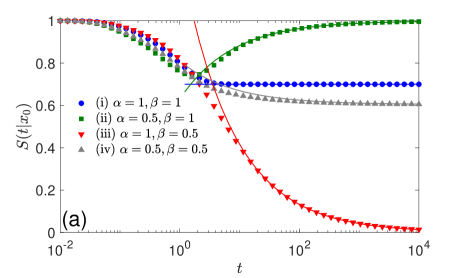
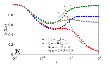
Figure 3: The probability $S(t|\bm{x}_{0})$ of finding the particle in the unbound state at time $t$, for diffusion between concentric spheres, with $D=1$, $R=1$, $|\bm{x}_{0}|=1.5$, $L=2$ (a) and $L=10$ (b). The random threshold and waiting time obey Mittag-Leffler distributions (87, 88), with $\ell_{0}=1$ and $t_{d}=1$ (a) and $\ell_{0}=0.1$ and $t_{d}=10$ (b), and four combinations of the exponents $\alpha$ and $\beta$ as indicated in the legend. Symbols present the inverse Laplace transform of the exact expression (79) obtained by the Talbot algorithm, whereas lines indicate the long-time asymptotic relations discussed in Sec. II.5. The values of $\ell_{0}$ and $t_{d}$ were changed for the panel (b) for a better visualization.

Figure 3 illustrates the behavior of the probability $S(t|\bm{x}_{0})$ of finding a particle in the unbound state in four different regimes discussed in Sec. II.5. Two panels correspond to strong and weak confinements, with $L=2$ and $L=10$, respectively. In both cases, the asymptotic relations derived in Sec. II.5 accurately capture the long-time behavior of $S(t|\bm{x}_{0})$. For the regimes (i), (iii) and (iv), $S(t|\bm{x}_{0})$ exhibits a monotonous decrease in panel (a); in contrast, this function achieves a minimum in the regime (ii). This minimum is necessarily present for any setting because $S(t|\bm{x}_{0})$ starts from $1$ at $t=0$ and returns to $1$ in the limit $t\to\infty$. In turn, the monotonous decrease of $S(t|\bm{x}_{0})$ in other regimes is specific to the chosen set of parameters. For instance, the panel (b) illustrates the case $L=10$, for which $S(t|\bm{x}_{0})$ is not monotonous in all regimes. Moreover, a local maximum is observed for the case (iv). Changing the parameters $\ell_{0}$ and $t_{d}$ (as well as $L$ and $|\bm{x}_{0}|$), one can achieve other situations (not shown), in which this local maximum is either enhanced or removed. To rationalize its origin, let us revise the short-time and long-time behaviors of the probability $S(t|\bm{x}_{0})$. At short times, the binding kinetics is the limiting factor so that $S(t|\bm{x}_{0})$ is almost independent of the unbinding kinetics (see Appendix D for technical details). In particular, a rapid decrease of $S(t|\bm{x}_{0})$ can be achieved either by increasing the “reactivity” of $\partial\Omega_{R}$ (i.e., taking smaller $\ell_{0}$ or $t_{a}$) or by choosing the starting position $\bm{x}_{0}$ closer to $\partial\Omega_{R}$. After this initial drop, unbinding events come in play and start to “compete” with binding events to slowly reach an equilibrium limit $S(\infty|\bm{x}_{0})=1/(1+(t_{d}/t_{a})^{\alpha})$. Changing the timescale $t_{d}$ of unbinding events allows one to control the value of this limit, independently of the short-time behavior. Moreover, as the second term in Eq. (78) is positive, the limit $S(\infty|\bm{x}_{0})$ is approached from above. As a consequence, if the initial drop led to intermediate values of $S(t|\bm{x}_{0})$ that are below $S(\infty|\bm{x}_{0})$, a local maximum should be present. In a similar way, one can rationalize the presence of a local maximum for the case (iii) that we observed for a different set of parameters (not shown).

III.4 Diffusive flux

In order to quantify the uptake on the reactive region, we consider the diffusive flux $J(t)$, which is obtained via a numerical inversion of the Laplace transform in Eq. (82). To grasp the main features of this quantity, we start with the conventional case of Markovian binding and unbinding kinetics (i.e., $\alpha=\beta=1$).

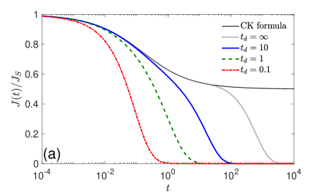
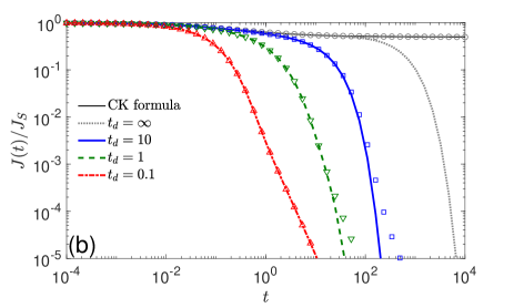
Figure 4: (a) The diffusive flux $J(t)$ divided by the Smoluchowski steady-state flux $J_{\rm S}$ from Eq. (99), for diffusion between concentric spheres, with $D=1$, $R=1$, $L=10$, and $c_{0}=1$. Conventional Markovian binding/unbinding kinetics ($\alpha=\beta=1$), with $\ell_{0}=1$ (and thus $q=1$) and four values of the mean waiting time $t_{d}$ as indicated in the legend. The classical Collins-Kimball formula (97) is compared to the inverse Laplace transform of the exact expression (86) obtained numerically by the Talbot algorithm. (b) The same diffusive fluxes are presented on the log-log scale, for $L=10$ (shown by lines, as on panel (a)) and $L=100$ (shown by symbols).

Figure 4(a) shows the diffusive flux $J(t)$ as a function of time $t$ for four values of the mean waiting time $t_{d}$. Let us first look at the particular case $t_{d}=\infty$ corresponding to irreversible binding. Comparing this curve with the explicit Collins-Kimball formula (97) for $L=\infty$ (shown by thin black line), one can clearly see the effect of confinement. At short times, two curves are almost indistinguishable because the flux is formed by particles near the reactive region and thus there is no influence of the outer reflecting boundary. However, as time goes on, two curves split and start to behave differently. Indeed, when there is no outer boundary, the confining domain is unbounded, and there is an infinite, inexhaustible amount of particles that diffuse toward the sphere to react on it. The flux reaches a strictly positive steady-state limit $J_{\rm S}\frac{qR}{1+qR}$, which depends on the reactivity parameter $q$. In contrast, if the domain is bounded, the amount of particles is limited, and they all irreversibly bind to the sphere so that the flux drops to $0$ as $t\to\infty$.

The presence of unbinding events (i.e., a finite value of $t_{d}$) does not fundamentally change the behavior but shifts the curves to shorter times as $t_{d}$ decreases. At first thought, this may sound counter-intuitive because unbinding events ensure that some particles are present in the confining domain; in particular, we saw earlier that the fraction of particles in the bulk reaches a constant. In this case, vanishing of the flux simply reflects that the equilibrium is reached at long times.

The remarkable effect of unbinding events is that the diffusive flux does not almost depend on the size $L$ of the confinement if the size is large enough. This is illustrated on Fig. 4(b) which compares the fluxes in two domains, with $L=10$ (lines) and $L=100$ (symbols). For irreversible binding, an enlargement of the domain to $L=100$ extends the validity of the Collins-Kimball formula to longer times, implying the deviation between two curves for $L=10$ and $L=100$. In contrast, when binding is reversible, the curves for $L=10$ and $L=100$ are almost indistinguishable. Actually, to see their difference at long times, we had to show the vertical axis in panel (b) on logarithmic scale. From the mathematical point of view, the similarity between these curves comes from the fact that the smallest eigenvalue $\mu_{0}^{(p)}$, given by Eq. (81), is exponentially close to its limiting value $1/R+\sqrt{p/D}$ when $L$ is large enough and $p$ is not too small (indeed, $\tanh((L-R)\sqrt{p/D})=1+O(exp)$ when $(L-R)\sqrt{p/D}\gg 1$). As a consequence, the effect of confinement can only be seen at very small $p$ or, equivalently, at very long times. From the physical point of view, if $L$ is large enough, the system starts to equilibrate near the reactive sphere (on a time scale of $t_{d}$), and then the equilibrated layer extends further into the bulk due to diffusion. As a consequence, the initial drop of the diffusive flux $J(t)$ on the reactive sphere does not depend on the confinement size.

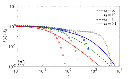
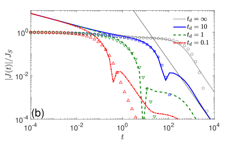
Figure 5: The diffusive flux $J(t)$ divided by the Smoluchowski steady-state flux $J_{\rm S}$ from Eq. (99), for diffusion between concentric spheres, with $D=1$, $R=1$, $L=10$, and $c_{0}=1$, and Mittag-Leffler binding/unbinding kinetics determined by (87, 88), with $\ell_{0}=1$ and four values of the time scale $t_{d}$ as indicated in the legend. Symbols present the reference case of Markovian binding/unbinding kinetics ($\alpha=\beta=1$). Lines show non-Markovian cases: (a) $\alpha=1$, $\beta=0.5$; (b) $\alpha=0.5$, $\beta=1$; and (c) $\alpha=0.5$, $\beta=0.5$. Black straight line on panel (b) presents the long-time asymptotic relation (106) for $t_{d}=10$.

Figure 5 illustrates the effects of non-Markovian binding and unbinding kinetics. To highlight these effects, we consider the aforementioned Markovian kinetics as a reference case (shown by symbols). We also fix the threshold scale $\ell_{0}=1$ and use the same set of time scales $t_{d}$ as in Fig. 4. Panel (a) presents the effect of non-Markovian unbinding kinetics ($\alpha=1,~{}\beta=0.5$). When $t_{d}=\infty$ (irreversible binding), the unbinding kinetics has no influence, and two curves (for $\beta=0.5$ and $\beta=1$) are identical. In turn, there is a drastic difference between the cases $\beta=0.5$ and $\beta=1$ for any finite $t_{d}$. In fact, anomalously long sojourns in the bound state considerably delay the decay of the diffusive flux and thus the equilibration of the system. In line with the long-time asymptotic analysis of Sec. II.5, one can easily show that the exponential decay for $\beta=1$ switches to a power-law decay for $\beta=0.5$. These qualitative conclusions agree with the earlier results by Agmon and Weiss for the unbounded case $L=\infty$ [86].

In turn, panel (b) of Fig. 5 presents the new effect of non-Markovian binding kinetics, while keeping the unbinding events to be Markovian ($\alpha=0.5,~{}\beta=1$). Let us first examine the short-time behavior. As the mean threshold is infinite in the case $\alpha=0.5$, binding events are expected to be rarer, as compared to the case of Markovian binding with $\alpha=1$, and therefore it would be more difficult for a particle to adsorb on the substrate. One might thus expect that the diffusive flux would be smaller for $\alpha=0.5$ than for $\alpha=1$. This is not the case. In contrast, while the diffusive flux converged to a constant as $t\to 0$ for the Markovian binding kinetics (in agreement with the Collins-Kimball formula), it diverges for the considered non-Markovian setting. In fact, substituting $\mu_{0}^{(p)}\approx\sqrt{p/D}$ and $\bar{\psi}(\mu)\approx(\mu\ell_{0})^{-\alpha}$ for large $p$ and $\mu$ into Eq. (82), one gets

$$\tilde{J}(p)\approx J_{\rm S}\frac{RD^{(\alpha-1)/2}}{\ell_{0}^{\alpha}}\,p^{-(\alpha+1)/2}\quad(p\to\infty),$$ (103)

from which

$$J(t)\approx J_{\rm S}\frac{R\,(Dt/\ell_{0}^{2})^{(\alpha-1)/2}}{\ell_{0}\,\Gamma(\frac{\alpha+1}{2})}\quad(t\to 0),$$ (104)

in agreement with the power-law divergence seen in Fig. 5(b). Expectedly, the short-time behavior does not depend on the unbinding kinetics so that four curves for different $t_{d}$ fall onto each other.

What is the reason of this enhanced flux? We recall that the encounter-based description identifies the binding event with the first crossing of the random threshold $\hat{\ell}$ by the boundary local time. According to Eq. (90a), small values of the threshold $\hat{\ell}$ are more likely than in the Markovian model. As a consequence, the particle can easier bind the reactive region at short times within the Mittag-Leffler model. Evidently, this peculiar result is specific to the small-$\ell$ behavior of the probability density $\psi(\ell)$. In [106], other models were discussed, for which the diffusive flux may tend zero as $t\to 0$. We finally note that the strongest divergence $J(t)\propto t^{-1/2}$ corresponds to the formal limit $\alpha=0$, which corresponds to the Smoluchowski setting of a perfect adsorption, see Eq. (98).

The long-time behavior of the diffusive flux on Fig. 5(b) reveals another interesting feature. At intermediate times, the curves for $\alpha=0.5$ are close to those for $\alpha=1$ suggesting that the distinction between Markovian and non-Markovian binding kinetics is progressively reduced due to several binding/unbinding events. However, at longer times, the curves separate again and become drastically different. In particular, one can notice a spike-like feature which actually means that the diffusive flux becomes negative (note also that the absolute value of the diffusive flux is plotted on this panel, to be able to employ the logarithmic scale on the vertical axis). The negative values of the diffusive flux can be also deduced from the long-time asymptotic analysis from Sec. II.5. Repeating it for the diffusive flux, one gets

$$\tilde{J}(p)\approx J_{\rm S}\frac{Rt_{a}^{1-\alpha}t_{d}}{\ell_{0}}\,p^{1-\alpha}\quad(p\to 0),$$ (105)

so that

$$J(t)\approx J_{\rm S}\frac{Rt_{a}^{1-\alpha}t_{d}}{\ell_{0}\Gamma(\alpha-1)}\,t^{\alpha-2}\quad(t\to\infty).$$ (106)

Since $0<\alpha<1$, $\Gamma(\alpha-1)$ is negative, and so is the flux at long times. This behavior can be intuitively expected. At the beginning, there is no particle in the bound state, and eventual binding events are responsible for the positive flux at short and intermediate times. However, the power-law decay in Eq. (90b) allows for anomalously large values of the random threshold $\hat{\ell}$ so that binding events are getting rarer and rarer in the course of time. As a consequence, the bound particles start to be released more often than the new ones are getting bound, implying the negative flux. The power-law decay (106) implies that the equilibration of the system is anomalously long. We stress that the negative flux can be also found in the Markovian setting; it is actually related to the non-monotonous behavior of the probability $S(t|\bm{x}_{0})$ (see, e.g., the curve shown by blue circles on Fig. 3(b)).

The last panel (c) of Fig. 5 illustrates the combined effect of both non-Markovian binding and unbinding kinetics ($\alpha=\beta=0.5$). Expectedly, the short-time behavior has not changed as being unaffected by unbinding kinetics. In turn, the long-time behavior is again modified. In this particular example, the diffusive flux remains positive for all times but still exhibits a slow power-law decay. Its positive character simply reflects a sort of balance between anomalously rare binding events and anomalously long durations of unbinding events.

III.5 Concentration evolution

Yet another insight onto reversible diffusion-controlled reactions can be achieved by looking at the temporal evolution of the concentration profile $c(\bm{x},t)$ from the uniform initial concentration $c_{0}$. We recall that this quantity is proportional to the probability $S(t|\bm{x})$ and is a function of the radial distance $r=|\bm{x}|$ for the considered spherical domain. Figure 6 illustrates how the concentration evolves with time for four combinations of the exponents $\alpha$ and $\beta$ (all other parameters being kept fixed to ease the comparison). In the conventional setting $\alpha=\beta=1$ (panel (a)), one observes an exponential approach to the equilibrium concentration, $c_{0}/(1+t_{d}/t_{a})=0.7$, as discussed in Sec. II.5. When the unbinding kinetics is non-Markovian (panel (b)), the particles stay longer and longer in the bound state so that the concentration of unbound particles slowly vanishes. In turn, if the binding kinetics is non-Markovian (panel (c)), binding events are rare at long times, and the concentration is slowly restored to the initial level $c_{0}$. Finally, when both kinetics are non-Markovian (panel (d)), the rarity of binding and unbinding events is compensated and leads to a slow relaxation to a new equilibrium concentration, $c_{0}/(1+(t_{d}/t_{a})^{\alpha})\approx 0.60$.

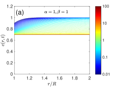
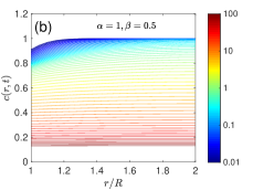
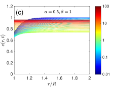
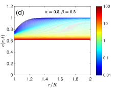
Figure 6: The concentration profile $c(\bm{x},t)$ (rescaled by $c_{0}$) as a function of $r=|\bm{x}|$, for diffusion between concentric spheres, with $D=1$, $R=1$, $L=2$, $c_{0}=1$, and the Mittag-Leffler binding/unbinding kinetics determined by (87, 88), with $\ell_{0}=1$ and $t_{d}=1$. The concentration was evaluated at 64 times ranging uniformly on the logarithmic scale from $0.01$ to $100$ and represented by colors, from dark blue ($t=0.01$) to dark red ($t=100$). (a) $\alpha=1$, $\beta=1$; (b) $\alpha=1$, $\beta=0.5$; (c) $\alpha=0.5$, $\beta=1$; and (d) $\alpha=0.5$, $\beta=0.5$.

IV Discussion

Despite successful applications of the conventional (Markovian) binding/unbinding kinetics, its numerous limitations have been identified long ago. For instance, Agmon and Weiss introduced a general waiting time distribution to account for anomalously long sojourns in the bound states [86]. Similarly, the simple form of the forward reaction term in Eq. (5) cannot fully account for microscopic heterogeneity of the reactive region, its temporal variations, saturation effects in adsorption processes and passivation of catalysts, as well as various regulation and control mechanisms of biochemical reactions in living cells. Quite naturally, different extensions of the forward term have been proposed. Here we briefly discuss a large class of extensions that impact reactivity but do not alter the linearity of the forward term with respect to $c(\bm{x},t)$.

There are at least three basic ways to render reactivity nonconstant (and thus to go beyond the classical setting): (i) a space-dependent reactivity $\kappa(\bm{x})$ that allows one to model microscopic heterogeneity of the reactive region; (ii) a time-dependent reactivity $\kappa(t)$ that implements a temporal evolution of that region; and (iii) a $p$-dependent reactivity $\tilde{\kappa}(p)$ in the Laplace domain that incorporates memory effects via a convolution-type boundary condition (10) in time domain (one can also consider their combinations). The first extension is in general challenging because the diffusive dynamics is intrinsicly coupled here to surface reactions: the particle encounters the reactive region in different locations and thus realizes a sequence of reaction attempts with different reaction probabilities that depend on the whole random trajectory of the particle. A general spectral approach for this extension was proposed in [125] (see further discussions and references therein). The second extension is also difficult for analytical treatments because the Laplace transform, which is usually performed to reduce the diffusion equation to the modified Helmholtz equation, would lead to a convolution-type Robin boundary condition in the Laplace domain. In contrast, the third extension, that we discussed in Sec. II.3, does not change the solution in the Laplace domain, except that the constant reactivity $\kappa_{0}$ is replaced by the reactivity $\tilde{\kappa}(p)$ that depends on $p$ as a fixed parameter. In turn, the asymptotic behavior of the solution, as well as its form in time domain, are modified.

The general binding mechanism discussed in this paper can be associated to the fourth extension of a constant reactivity. As first suggested in [106], the probability density $\psi(\ell)$ of the threshold $\hat{\ell}$ can be related to the so-called encounter-dependent reactivity as

$$\kappa(\ell)=D\frac{\psi(\ell)}{\int\nolimits_{\ell}^{\infty}d\ell^{\prime}\,\psi(\ell^{\prime})}\,.$$ (107)

In the conventional setting, the particle attempts to react at each arrival onto $\partial\Omega_{R}$ with the constant probability $\rho\approx a\kappa_{0}/D$ (see Sec. II.1). In turn, Eq. (107) allows one to implement an arbitrary dependence of the reaction probability on the number of encounters, i.e., on the number of failed attempts represented by $\ell$. The encounter-dependent reactivity can be interpreted in a similar way to the time-dependent diffusivity $D(t)$ [145, 146, 147]. In fact, if the bulk properties change with time, their effect onto diffusive displacements can be modeled via a prescribed dependence $D(t)$. Likewise, if the reactive properties of the substrate depend on the number of encounters with the particle, it can be modeled via a prescribed dependence $\kappa(\ell)$. This is yet another manifestation of the fundamental similarity between the physical time as a proxy of the number of bulk jumps and the boundary local time as a proxy of the number of jumps onto the boundary.

To illustrate the concept of the encounter-dependent reactivity, let us inspect again the Mittag-Leffler model. Inserting Eq. (87) for the probability density $\psi(\ell)$ in Eq. (107), one gets

$$\kappa(\ell)=\kappa_{0}(\ell/\ell_{0})^{\alpha-1}\frac{E_{\alpha,\alpha}(-(\ell/\ell_{0})^{\alpha})}{E_{\alpha,1}(-(\ell/\ell_{0})^{\alpha})}\,,$$ (108)

with $\kappa_{0}=D/\ell_{0}$. This function is shown on Fig. 2(b). In the Markovian case $\alpha=1$, one simply retrieves a constant reactivity $\kappa(\ell)=\kappa_{0}$, which stands in the Robin boundary condition (1). In turn, if $0<\alpha<1$, the above encounter-dependent reactivity exhibits two asymptotic power-law behaviors

$$\kappa(\ell) \approx\frac{\kappa_{0}}{\Gamma(\alpha)}(\ell/\ell_{0})^{\alpha-1}\quad(\ell\to 0),$$ (109a)

$$\kappa(\ell) \approx\kappa_{0}\alpha(\ell/\ell_{0})^{-1}\quad(\ell\to\infty).$$ (109b)

In the limit $\ell\to 0$, the encounter-dependent reactivity diverges, indicating that $\partial\Omega_{R}$ is highly reactive. This is consistent with the earlier discussion that small values of the threshold $\hat{\ell}$ are more likely to occur than for the Markovian setting with $\alpha=1$. The higher reactivity can thus explain the larger diffusive flux observed in Fig. 5(b). In the opposite limit $\ell\to\infty$, the reactivity slowly decays, resulting in rarer and rarer binding events. While we focused on the Mittag-Leffler model for illustrative purposes, one can easily implement any function $\kappa(\ell)$, which is suitable to represent the reactivity evolution of the substrate, by using the random threshold with the probability density

$$\psi(\ell)=\frac{\kappa(\ell)}{D}\exp\left(-\frac{1}{D}\int\limits_{0}^{\ell}d\ell^{\prime}\,\kappa(\ell^{\prime})\right).$$ (110)

In other words, there is a mapping between $\kappa(\ell)$ and $\psi(\ell)$. In [106], several other models and their consequences for irreversible surface reactions were discussed.

We emphasize that $\kappa(\ell)$ depends on the number of encounters (represented by $\ell$), not on the physical time $t$. In other words, we model here the dynamical situation when the reactivity of the target $\partial\Omega_{R}$ changes due to its “interactions” with the particle, and not because of some external actions. We also stress that the effect of the encounter-dependent reactivity $\kappa(\ell)$ onto diffusion-controlled reactions is not in general reduced to a $p$-dependent reactivity $\tilde{\kappa}(p)$ or to a convolution-type boundary condition (10) with a memory kernel $\mathcal{K}(t)$, discussed in II.3. This reduction is only possible for some quantities and some specific geometric settings such as the spherical target considered in Sec. III.

In order to improve the intuitive comprehension of the general binding mechanism, let us further highlight its similarity with the description of unbinding events. In fact, the long history of continuous-time random walks gets us used to the concept of waiting times with heavy-tailed distributions and the consequent anomalous features [148, 149, 150]. One can formally say that an unbinding event occurs at the first instance $\tau$ when the time spent by the particle in the bound state exceeds a random threshold $\hat{\tau}$ obeying a given probability density $\phi(t)$:

$$\tau=\inf\{t>0~{}:~{}t>\hat{\tau}\}.$$ (111)

However, this is a tautology because $\tau=\hat{\tau}$. At the same time, this formal definition provides a direct analogy to the introduction of the first instance of a binding event via Eq. (18). As the boundary local time $\ell_{t}$ is the proxy of the number of encounters between the particle and the reactive region, the sequence of failed reaction attempts is stopped when $\ell_{t}$ exceeds an appropriate random threshold $\hat{\ell}$ with a given probability density $\psi(\ell)$. In this light, both binding and unbinding events are implemented in the same way, with the only difference that the “counter” of failed unbinding attempts is the physical time $t$, whereas the “counter” of failed binding attempts is the boundary local time $\ell_{t}$. While the impact of the waiting time and thus of a “threshold” $\hat{\tau}$ onto diffusive processes had been studied for many decades, the very similar threshold $\hat{\ell}$ for binding events, which was introduced in [61, 62, 139, 106], has not yet got a proper attention.

V Conclusion

In this paper, we developed a general theory of reversible diffusion-controlled reactions with general, non-Markovian binding and unbinding kinetics. In this theory, surface reactions are described by two functions: the probability density $\phi(t)$ that characterizes the random waiting time of a particle in the bound state, and the probability density $\psi(\ell)$ of the random number of failed reaction attempts prior to the successful binding. While an extension of the classical theory of reversible reactions to unbinding events with a general waiting time distribution was proposed by Agmon and Weiss more than thirty years ago [86], an implementation of non-Markovian binding events required recent advances on the encounter-based approach [106]. Combining this approach with the renewal technique, we managed to derive the spectral expansion (40) for the Laplace-transformed propagator $\tilde{Q}(\bm{x},p|\bm{x}_{0})$. When both $\phi(t)$ and $\psi(\ell)$ are exponential, one retrieves the Markovian setting with conventional forward rate constant $k_{\rm on}$ (or $\kappa_{0}$) and backward rate $k_{\rm off}$. From the propagator, we deduced other quantities such as the concentration of particles and the diffusive flux onto the reactive region. While spectral expansions are very common for describing diffusion-controlled reactions in bounded domains, they are usually based on the eigenmodes of the Laplace operator (or the Fokker-Planck operator) [9, 116, 117]. In turn, Eq. (40) employs the eigenmodes of the Dirichlet-to-Neumann operator $\mathcal{M}_{p}$, which is most suitable for describing diffusive exploration of the bulk between consecutive binding events. Being less known than the Laplace operator, the operator $\mathcal{M}_{p}$ offers flexible complementary tools for studying diffusion-controlled reactions.

As most formulas were derived in the Laplace domain, a numerical inversion of the Laplace transform was needed to present the results in time domain. Even without this inversion, the Laplace-transformed quantities allow one to determine the asymptotic behavior at short and long times. Moreover, if the diffusing particle has a random lifetime $\delta$ (so-called “mortal” random walker [151, 152, 153, 154]), the Laplace-transformed quantities admit additional probabilistic interpretations. For instance,

$$p\tilde{Q}(\bm{x},p|\bm{x}_{0})=\int\limits_{0}^{\infty}dt\,pe^{-pt}\,Q(\bm{x},t|\bm{x}_{0})=\mathbb{E}\{Q(\bm{x},\delta|\bm{x}_{0})\}$$ (112)

is the probability density of finding the particle in a vicinity of a bulk point $\bm{x}$ at the death time $\delta$, where $pe^{-pt}$ is the probability density of $\delta$ with the rate $p$. In other words, one does not need to perform the inverse Laplace transform in the framework of mortal random walkers.

When the binding kinetics is Markovian, the effect of non-Markovian unbinding events is captured in the Laplace domain via a $p$-dependent reactivity $\tilde{\kappa}(p)$, which is related by Eq. (50) to the probability density $\phi(t)$. In time domain, one retrieves thus a convolution-type boundary condition (10) with a memory kernel $\mathcal{K}(t)=\kappa_{0}\bigl{(}\delta(t)-\phi(t)\bigr{)}$. This result was already reported by Agmon and Weiss for the specific case of a spherical target [86]. Our approach permitted to generalize it to arbitrary bounded domains. In turn, when the binding kinetics is non-Markovian, the natural description of binding events involves the encounter-dependent reactivity $\kappa(\ell)$. In general, its effects are not reducible to an effective $\tilde{\kappa}(p)$ or to a memory kernel $\mathcal{K}(t)$. Further exploration of its effects and potentials for describing realistic surface reactions presents an important perspective for the future.

We also investigated the long-time behavior of the propagator $Q(\bm{x},t|\bm{x}_{0})$ and related quantities. Depending on the exponents $\alpha$ and $\beta$ that characterize the asymptotic behavior of the densities $\psi(\ell)$ and $\phi(t)$, four regimes were distinguished. When $\alpha=\beta=1$, one retrieves the classical exponential relaxation toward the uniform equilibrium state. If $\alpha<\beta$, binding events occur rarer than unbinding ones at long times so that the particle will be asymptotically in the unbound state; in turn, the opposite inequality $\alpha>\beta$ makes binding events more frequent so that the particle will be mostly in the bound state. Finally, if $\alpha=\beta<1$, a subtle balance between anomalously rare binding and unbinding events is settled, and a new uniform equilibrium state is approached anomalously slowly.

In order to highlight the effects of non-Markovian binding/unbinding kinetics, we considered the most basic setting of a single particle undergoing ordinary diffusion in the bulk. This study can be extended in several directions. (i) The ordinary bulk diffusion can be replaced by more general stochastic processes such as continuous-time random walks [148, 149, 150], processes with diffusing diffusivity [155, 156, 34], diffusion with a drift or in an external potential [157] diffusion with stochastic resetting [158, 159, 160], or in the presence of escape regions [161]. (ii) The collective effect of multiple independently diffusing particles can be implemented by defining binding events through the total boundary local time that these particles spent on the reactive region [162]. (iii) When the reactive region is bounded, the encounter-based approach can be used even for unbounded domains (see [143]); however, as briefly discussed in Sec. III.2, the long-time behavior can be considerably altered. (iv) In the case of a small reactive region, one can employ matched asymptotic techniques and other approximations [163, 164] to capture more explicitly the effects of non-Markovian binding/unbinding kinetics. (v) The majority of former contributions to reversible diffusion-controlled reactions dealt either with one-dimensional setting (diffusion on a half-line or, equivalently, diffusion in the half-space), or with diffusion outside a reactive sphere. The symmetry of these domains helped to implement adsorption/desorption kinetics rather explicitly (e.g., see Sec. III), but did not allow one to fully explore new features related to the encounter-dependent reactivity. In the future, it would be interesting to investigate how non-Markovian binding kinetics may affect diffusion-controlled reactions in more general confining domains.

Data Availability Statement

Data sharing is not applicable to this article as no new data were created or analyzed in this study.

Appendix A A microscopic derivation of Robin boundary conditions

In this Appendix, we provide a simple derivation of Robin-type boundary conditions for reversible binding in the conventional case of Markovian binding and unbinding kinetics. While the origins of Robin boundary condition and its microscopic interpretations for irreversible reactions have been thoroughly discussed [52, 165, 166, 62, 63, 50, 167, 168, 169], we propose here a simple derivation that may be instructive for non-expert readers.

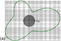
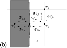
Figure 7: (a) A confining domain $\Omega\subset\mathbb{R}^{d}$ in two dimensions ($d=2$) is discretized by a square lattice. (b) A zoom of the vicinity of a boundary point $\bm{x}_{b}$, which is connected to a single bulk point $\bm{x}_{i}$ in the interior and to a storage site $\bm{x}_{s}$. Some transition rates $W$ between connected sites are shown.

To get an intuitive picture of Robin boundary conditions, let us approximate Brownian motion by a symmetric random walk on a $d$-dimensional (hyper)cubic lattice with a step $a$ that discretizes the confining domain $\Omega$ (Fig. 7(a)). As surface reactions are local in space, it is sufficient to consider a vicinity of a boundary point $\bm{x}_{b}$ on $\partial\Omega_{R}$ (Fig. 7(b)). For the sake of simplicity, we assume that this point is connected to a single bulk point $\bm{x}_{i}$ in the interior of the domain (at distance $a$ from $\bm{x}_{b}$). As the binding event consists in a temporal “storage” of the particle on the boundary, the surface point $\bm{x}_{b}$ is also connected to a storage site $\bm{x}_{s}$ behind it. The diffusive dynamics of this random walk can be described by the master equation for the probability $q(\bm{x}_{k},t)$ of finding the particle in a state $\bm{x}_{k}$ at time $t$. For three aforementioned sites, the master equation reads

$$\frac{dq(\bm{x}_{s},t)}{dt} =-q(\bm{x}_{s},t)W_{s,b}+q(\bm{x}_{b},t)W_{b,s},$$ (113a)

$$\frac{dq(\bm{x}_{b},t)}{dt} =-q(\bm{x}_{b},t)\bigl{[}W_{b,s}+W_{b,i}\bigr{]}$$

$$+q(\bm{x}_{i},t)W_{i,b}+q(\bm{x}_{s},t)W_{s,b},$$ (113b)

$$\frac{dq(\bm{x}_{i},t)}{dt} =-q(\bm{x}_{i},t)\sum_{j}W_{i,j}+\sum_{j}q(\bm{x}_{j},t)W_{j,i},$$ (113c)

where the sums in the last relation are taken over all $2d$ neighbors $\bm{x}_{j}$ of the bulk site $\bm{x}_{i}$, and $W_{i,j}$ denotes the transition rate from site $i$ to site $j$. For bulk diffusion, one has

$$W_{j,i}=W_{i,j}=\frac{1}{2d\delta}\,,$$ (114)

where $\delta$ is a time step of one jump. The last master equation (113c) is the discrete version of the diffusion equation with

$$D=\frac{a^{2}}{2d\delta}\,.$$ (115)

Using this relation, the second master equation (113b) can be written as

$$\frac{dq(\bm{x}_{b},t)}{dt} =-\frac{D}{a}\bigl{(}\partial_{n}q(\bm{x},t)\bigr{)}_{\bm{x}=\bm{x}_{b}}$$

$$-q(\bm{x}_{b},t)W_{b,s}+q(\bm{x}_{s},t)W_{s,b},$$

where we replaced the discretized form of the normal derivative, $(q(\bm{x}_{i},t)-q(\bm{x}_{b},t))/a$, by its continuous form. Substituting $W_{s,b}=k_{\rm off}$ and dividing by $a^{d-1}$, we get

$$a\frac{dc(\bm{x}_{b},t)}{dt} =-D\bigl{(}\partial_{n}c(\bm{x},t)\bigr{)}_{\bm{x}=\bm{x}_{b}}$$

$$-\kappa_{0}c(\bm{x}_{b},t)+k_{\rm off}c_{b}(\bm{x}_{b},t),$$ (116)

where we set

$$\kappa_{0}=aW_{b,s}$$ (117)

and introduced the bulk and surface concentrations as

$$c(\bm{x},t)=N_{0}\frac{q(\bm{x},t)}{a^{d}},\quad c_{b}(\bm{x}_{b},t)=N_{0}\frac{q(\bm{x}_{s},t)}{a^{d-1}}.$$ (118)

Here we included the number $N_{0}$ of independent diffusing particles to pass from a single-molecule description to the macroscopic one (expectedly, the surface concentration has the units 1/m^d-1 or mol/m^d-1). Note also that the storage site $\bm{x}_{s}$ was identified with the associated boundary site $\bm{x}_{b}$. In the limit $a\to 0$, the left-hand side of Eq. (116) vanishes, and one gets the boundary condition

$$-D\partial_{n}c(\bm{x},t)=\kappa_{0}\,c(\bm{x},t)-k_{\rm off}\,c_{b}(\bm{x},t)\quad(\bm{x}\in\partial\Omega_{R}).$$ (119)

Finally, the division of the first master equation (113a) by $a^{d-1}$ yields

$$\frac{dc_{b}(\bm{x}_{b},t)}{dt}=-k_{\rm off}\,c_{b}(\bm{x}_{b},t)+\kappa_{0}\,c(\bm{x}_{b},t),$$ (120)

which is identical to Eq. (5). In turn, the combination of Eqs. (119, 120) yields Eq. (6).

When there is no unbinding event (i.e., $k_{\rm off}=0$), the particle stays in the bound state forever, and Eq. (119) is reduced to the conventional Robin boundary condition. Here, the left-hand side is the diffusive flux from the bulk to the boundary (i.e., from $\bm{x}_{i}$ to $\bm{x}_{b}$ in the discrete picture), whereas the right-hand side is the “reactive flux” into the bound state (i.e., from $\bm{x}_{b}$ to $\bm{x}_{s}$ in the discrete picture).

The implicit assumption in the above derivation of the Robin-type boundary condition is that the transition rate $W_{b,s}$ to the bound state scales as $1/a$ in the limit $a\to 0$, in order to get a finite reactivity $\kappa_{0}$ in Eq. (117). A more general scaling

$$W_{b,s}\sim a^{-\gamma}\quad(a\to 0)$$ (121)

with $\gamma>1$ would yield an infinite reactivity and thus the Dirichlet boundary condition $c(\bm{x},t)=0$ at $\bm{x}\in\partial\Omega_{R}$. Once the particle hits such a point, it is immediately adsorbed. Moreover, as the desorption occurs at the same boundary point, the unbound particle re-binds immediately. In other words, this scaling leads to a perfect irreversible binding, regardless the unbinding kinetics. In turn, scaling (121) with $\gamma<1$ yields $\kappa_{0}=0$, i.e., an inert reflecting boundary. As the particle started from the unbound state, one has $c_{b}(\bm{x},0)=0$ and thus the diffusive flux remains zero at all times. We stress that the scaling relation (117) is indeed an assumption, in the same way as the scaling relation (115) for the diffusion coefficient: if Eq. (115) does not hold, the master equation does not converge to the macroscopic diffusion equation; similarly, if Eq. (117) is not valid, the macroscopic limit does not represent a partially reactive boundary.

Appendix B Distribution of binding times

The probability flux density $j_{\psi}(\bm{x},t|\bm{x}_{0})$ can be interpreted as the joint probability density of the binding position $\bm{X}_{\mathcal{T}}$ and the binding time $\mathcal{T}$ defined by Eq. (18). In particular, the integral of this quantity over $\bm{x}\in\partial\Omega_{R}$ determines the (marginal) probability density of the binding time

$$J_{\psi}(t|\bm{x}_{0})=\int\limits_{\partial\Omega_{R}}d\bm{x}\,j_{\psi}(\bm{x},t|\bm{x}_{0}).$$ (122)

As a consequence, the spectral expansion (36) implies

$$\tilde{J}_{\psi}(p|\bm{x}_{0}) =\mathbb{E}_{\bm{x}_{0}}\{e^{-p\mathcal{T}}\}$$

$$=\sum\limits_{k=0}^{\infty}[V_{k}^{(p)}(\bm{x}_{0})]^{*}\bar{\psi}(\mu_{k}^{(p)})\int\limits_{\partial\Omega_{R}}d\bm{x}\,v_{k}^{(p)}(\bm{x})\,.$$ (123)

This quantity determines all positive integer-order moments of the binding time $\mathcal{T}$ (if they exist),

$$\mathbb{E}_{\bm{x}_{0}}\{\mathcal{T}^{n}\}=(-1)^{n}\lim\limits_{p\to 0}\frac{\partial^{n}}{\partial p^{n}}\tilde{J}_{\psi}(p|\bm{x}_{0}),$$ (124)

while its inverse Laplace transform yields the probability density $J(t|\bm{x}_{0})$.

Let us examine the small-$p$ asymptotic behavior of Eq. (123) by treating separately the contributions from the ground eigenmode $k=0$ and other eigenmodes with $k>0$. In fact, as $v_{0}^{(p)}$ approaches a constant in the limit $p\to 0$, the integral in Eq. (123) vanishes for any $k>0$. Substituting the small-$p$ expansion (64) for $k=0$, we get

$$\tilde{J}_{\psi}(p|\bm{x}_{0})\approx 1-p^{\alpha}t_{a}^{\alpha}+O(p)\quad(p\to 0).$$ (125)

If $0<\alpha<1$, the correction $O(p)$ from all other terms is subleading, and the mean binding time is infinite. In this case, binding events are characterized by the time scale $t_{a}$ from Eq. (65). In contrast, if $\alpha=1$, both contributions in Eq. (125) are comparable and sum up to determine the mean binding time.

Appendix C Diffusion on an interval

In this Appendix, we summarize the formulas in the case of diffusion on an interval $(0,L)$, with the reactive endpoint $x=0$ and the reflecting endpoint $x=L$ [107]. In this case, Eqs. (80a, 81) are replaced by

$$g_{0}^{(p)}(x) =\frac{\cosh((L-x)\sqrt{p/D})}{\cosh(L\sqrt{p/D})}\,,$$ (126)

$$\mu_{0}^{(p)} =\sqrt{p/D}\,\tanh(L\sqrt{p/D}),$$ (127)

while other relations in the beginning of Sec. III remain unchanged, except for the diffusive flux, which reads

$$\tilde{J}(p)=(-D\partial_{n}\tilde{c}(x,p))_{x=0}=c_{0}D\frac{\mu_{0}^{(p)}(1-\tilde{\phi}(p))\bar{\psi}(\mu_{0}^{(p)})}{p[1-\tilde{\phi}(p)\bar{\psi}(\mu_{0}^{(p)})]}$$ (128)

and differs from Eq. (82) by the factor $4\pi R^{2}$ (the surface area of the reactive region). The major difference between these two settings araises in the limit $L\to\infty$ when the outer reflecting boundary is moved to infinity so that $\mu_{0}^{(p)}=\sqrt{p/D}$ on the half-line. As $p\to 0$, this eigenvalue vanishes, whereas the eigenvalue $\mu_{0}^{(p)}$ from Eq. (81) approached a strictly positive constant $1/R$ (see Sec. III). This distinction is related to the transient (resp. recurrent) character of three-dimensional (resp. one-dimensional) Brownian motions, see [143] for further discussions.

Appendix D Short-time behavior

We briefly discuss the short-time asymptotic behavior of $S(t|\bm{x}_{0})$ for the case of diffusion between concentric spheres. According to Eq. (80a, 81), one has $g_{0}^{(p)}(r_{0})\approx e^{-(r_{0}-R)\sqrt{p/D}}R/r_{0}$ and $\mu_{0}^{(p)}\approx\sqrt{p/D}$ in the limit $p\to\infty$. For the Mittag-Leffler model, one gets

$$\bar{\psi}(\mu)\approx(\ell_{0}\mu)^{-\alpha}\quad(\mu\to\infty),$$ (129)

and so that Eq. (79) implies

$$\tilde{S}(p|\bm{x}_{0})\approx\frac{1}{p}-e^{-(r_{0}-R)\sqrt{p/D}}\frac{RD^{\alpha/2}}{r_{0}\ell_{0}^{\alpha}p^{1+\alpha/2}}\quad(p\to\infty).$$ (130)

Expectedly, this behavior does not depend on the waiting time distribution. In fact, the particle does not have enough time to unbind in this limit, and the probability $S(t|\bm{x}_{0})$ at short times is mainly affected by the first binding event.

The inverse Laplace transform yields

$$S(t|\bm{x}_{0}) \approx 1-\frac{RD^{\alpha/2}}{r_{0}\ell_{0}^{\alpha}}\int\limits_{0}^{t}dt_{1}\,\frac{(r_{0}-R)e^{-(r_{0}-R)^{2}/(4Dt_{1})}}{\sqrt{4\pi Dt_{1}^{3}}}$$

$$\times\frac{(t-t_{1})^{\alpha/2}}{\Gamma(\alpha/2+1)}\quad(t\to 0).$$

After simplifications, we get

$$S(t|\bm{x}_{0})\approx 1-\frac{2^{1+\alpha}R\,e^{-(r_{0}-R)^{2}/(4Dt)}}{\sqrt{\pi}\,r_{0}\,\ell_{0}^{\alpha}\,(r_{0}-R)^{\alpha+1}}\,(Dt)^{\alpha+1/2}\quad(t\to 0).$$ (131)

One sees that the short-time behavior is controlled by the first arrival onto the reactive region (the typical exponential factor $e^{-(r_{0}-R)^{2}/(4Dt)}$ from the Lévy-Smirnov probability density of the first-passage time) and by small random thresholds, i.e., by the behavior of $\psi(\ell)$ as $\ell\to 0$. The chosen Mittag-Leffler distribution is responsible for the corrective power-law factor $t^{\alpha+1/2}$. We stress that if $\bar{\psi}(\mu)$ does not exhibit a power-law decay (129), the result will be different.

References

- [1] M. Smoluchowski, Versuch einer Mathematischen Theorie der Koagulations Kinetic Kolloider Lösungen, Z. Phys. Chem. 92U, 129-168 (1918).
- [2] S. A. Rice, Diffusion-limited reactions (Elsevier, Amsterdam, 1985).
- [3] J. E. House, Principles of chemical kinetics (Academic press, 2007).
- [4] R. Metzler, G. Oshanin, and S. Redner (Eds), First-Passage Phenomena and Their Applications (Singapore, World Scientific, 2014).
- [5] K. Lindenberg, R. Metzler, and G. Oshanin (Eds), Chemical Kinetics: Beyond the Textbook (World Scientific, New Jersey, 2019).
- [6] B. Alberts, A. Johnson, J. Lewis, D. Morgan, M. Raff, K. Roberts, and P. Walter, Molecular Biology of the Cell (Garland Science, New York, NY, 2014).
- [7] D. A. Lauffenburger and J. Linderman, Receptors: Models for Binding, Trafficking, and Signaling (Oxford University Press, Oxford, 1993).
- [8] P. C. Bressloff and J. M. Newby, Stochastic models of intracellular transport, Rev. Mod. Phys. 85, 135-196 (2013).
- [9] S. Redner, A Guide to First Passage Processes (Cambridge, Cambridge University press, 2001).
- [10] Z. Schuss, Brownian Dynamics at Boundaries and Interfaces in Physics, Chemistry and Biology (Springer, New York, 2013).
- [11] O. Bénichou, C. Chevalier, J. Klafter, B. Meyer, and R. Voituriez, Geometry-controlled kinetics, Nat. Chem. 2, 472-477 (2010).
- [12] O. Bénichou and R. Voituriez, From first-passage times of random walks in confinement to geometry-controlled kinetics, Phys. Rep. 539, 225-284 (2014).
- [13] G. Vaccario, C. Antoine, and J. Talbot, First-Passage Times in d-Dimensional Heterogeneous Media, Phys. Rev. Lett. 115, 240601 (2015).
- [14] D. S. Grebenkov, Universal formula for the mean first passage time in planar domains, Phys. Rev. Lett. 117, 260201 (2016).
- [15] A. Godec and R. Metzler, First passage time distribution in heterogeneity controlled kinetics: going beyond the mean first passage time, Sci. Rep. 6, 20349 (2016).
- [16] M. Galanti, D. Fanelli, S. D. Traytak, and F. Piazza, Theory of diffusion-influenced reactions in complex geometries, Phys. Chem. Chem. Phys. 18, 15950-15954 (2016).
- [17] T. Kolokolnikov, M. S. Titcombe, and M. J. Ward, Optimizing the fundamental Neumann eigenvalue for the Laplacian in a domain with small traps, Eur. J. Appl. Math 16, 161 (2005).
- [18] A. Singer, Z. Schuss, D. Holcman, and R. S. Eisenberg, Narrow escape, part I, J. Stat. Phys. 122, 437-463 (2006).
- [19] A. Singer, Z. Schuss, and D. Holcman, Narrow escape, part II: the circular disk, J. Stat. Phys. 122, 465 (2006).
- [20] A. Singer, Z. Schuss, and D. Holcman, Narrow escape, part III: non-smooth domains and Riemann surfaces, J. Stat. Phys. 122, 491 (2006).
- [21] Z. Schuss, A. Singer, and D. Holcman, The narrow escape problem for diffusion in cellular microdomains, Proc. Nat. Acad. Sci. USA 104, 16098-16103 (2007).
- [22] O. Bénichou and R. Voituriez, Narrow-escape time problem: time needed for a particle to exit a confining domain through a small window, Phys. Rev. Lett. 100, 168105 (2008).
- [23] S. Pillay, M. J. Ward, A. Peirce, and T. Kolokolnikov, An asymptotic analysis of the mean first passage time for narrow escape problems: part I: two-dimensional domains, Multiscale Model. Simul. 8, 803-835 (2010).
- [24] A. F. Cheviakov, M. J. Ward, and R. Straube, An asymptotic analysis of the mean first passage time for narrow escape problems: part II: the sphere, Multiscale Model. Simul. 8, 836-870 (2010).
- [25] A. F. Cheviakov and M. J. Ward, Optimizing the principal eigenvalue of the Laplacian in a sphere with interior traps, Math. Comput. Modelling 53, 1394-1409 (2011).
- [26] A. F. Cheviakov, A. S. Reimer, and M. J. Ward, Mathematical modeling and numerical computation of narrow escape problems, Phys. Rev. E 85, 021131 (2012).
- [27] D. Holcman and Z. Schuss, Control of flux by narrow passages and hidden targets in cellular biology, Phys. Progr. Rep. 76, 074601 (2013).
- [28] D. Holcman and Z. Schuss, The narrow escape problem, SIAM Rev. 56, 213-257 (2014).
- [29] S. A. Isaacson, A. J. Mauro, and J. Newby, Uniform asymptotic approximation of diffusion to a small target: Generalized reaction models, Phys. Rev. E 94, 042414 (2016).
- [30] D. S. Grebenkov and G. Oshanin, Diffusive escape through a narrow opening: new insights into a classic problem, Phys. Chem. Chem. Phys. 19, 2723-2739 (2017).
- [31] D. S. Grebenkov, R. Metzler, and G. Oshanin, Effects of the target aspect ratio and intrinsic reactivity onto diffusive search in bounded domains, New J. Phys. 19, 103025 (2017).
- [32] T. Agranov and B. Meerson, Narrow escape of interacting diffusing particles, Phys. Rev. Lett. 120, 120601 (2018).
- [33] S. Condamin, O. Bénichou, V. Tejedor, R. Voituriez, and J. Klafter, First-passage time in complex scale-invariant media, Nature 450, 77 (2007).
- [34] Y. Lanoiselée, N. Moutal, and D. S. Grebenkov, Diffusion-limited reactions in dynamic heterogeneous media, Nature Commun. 9, 4398 (2018).
- [35] D. S. Grebenkov, Searching for partially reactive sites: Analytical results for spherical targets, J. Chem. Phys. 132, 034104 (2010).
- [36] D. S. Grebenkov, Subdiffusion in a bounded domain with a partially absorbing-reflecting boundary, Phys. Rev. E 81, 021128 (2010).
- [37] T. Guérin, N. Levernier, O. Bénichou, and R. Voituriez, Mean first-passage times of non-Markovian random walkers in confinement, Nature 534, 356-359 (2016).
- [38] T. G. Mattos, C. Mejía-Monasterio, R. Metzler, and G. Oshanin, First passages in bounded domains: When is the mean first passage time meaningful? Phys. Rev. E 86, 031143 (2012).
- [39] A. Godec and R. Metzler, Universal Proximity Effect in Target Search Kinetics in the Few-Encounter Limit, Phys. Rev. X 6, 041037 (2016).
- [40] D. S. Grebenkov, R. Metzler, and G. Oshanin, Strong defocusing of molecular reaction times results from an interplay of geometry and reaction control, Commun. Chem. 1, 96 (2018).
- [41] D. S. Grebenkov, R. Metzler, and G. Oshanin, Towards a full quantitative description of single-molecule reaction kinetics in biological cells, Phys. Chem. Chem. Phys. 20, 16393-16401 (2018).
- [42] D. S. Grebenkov, R. Metzler, and G. Oshanin, Full distribution of first exit times in the narrow escape problem, New J. Phys. 21, 122001 (2019).
- [43] F. C. Collins and G. E. Kimball, Diffusion-controlled reaction rates, J. Colloid Sci. 4, 425 (1949).
- [44] H.-X. Zhou and R. Zwanzig, A rate process with an entropy barrier, J. Chem. Phys. 94, 6147 (1991).
- [45] D. Reguera, G. Schmid, P. S. Burada, J.-M. Rubí, P. Reimann, and P. Hänggi, Entropic Transport: Kinetics, Scaling, and Control Mechanisms, Phys. Rev. Lett. 96, 130603 (2006).
- [46] P. Malgaretti, I. Pagonabarraga and J. Miguel Rubí, Entropically induced asymmetric passage times of charged tracers across corrugated channels, J. Chem. Phys. 144, 034901 (2016).
- [47] A. T. Skvortsov, L. Dagdug, E. F. Hilder, A. M. Berezhkovskii, and S. M. Bezrukov, Permeability and diffusion resistance of porous membranes: Analytical theory and its numerical test, J. Chem. Phys. 158, 054114 (2023).
- [48] O. Bénichou, M. Moreau, and G. Oshanin, Kinetics of stochastically gated diffusion-limited reactions and geometry of random walk trajectories, Phys. Rev. E 61, 3388-3406 (2000).
- [49] J. Reingruber and D. Holcman, Gated Narrow Escape Time for Molecular Signaling, Phys. Rev. Lett. 103, 148102 (2009).
- [50] S. D. Lawley and J. P. Keener, A new derivation of Robin boundary conditions through homogenization of a stochastically switching boundary, SIAM J. Appl. Dyn. Syst. 14, 1845-1867 (2015).
- [51] P. C. Bressloff, Stochastic switching in biology: from genotype to phenotype, J. Phys. A. 50, 133001 (2017).
- [52] H. C. Berg and E. M. Purcell, Physics of chemoreception, Biophys. J. 20, 193 (1977).
- [53] D. Shoup, G. Lipari, and A. Szabo, Diffusion-controlled bimolecular reaction rates. The effect of rotational diffusion and orientation constraints, Biophys. J. 36, 697-714 (1981).
- [54] R. Zwanzig and A. Szabo, Time dependent rate of diffusion-influenced ligand binding to receptors on cell surfaces, Biophys. J. 60, 671-678 (1991).
- [55] A. M. Berezhkovskii, M. I. Monine, C. B. Muratov, and S. Y. Shvartsman, Homogenization of boundary conditions for surfaces with regular arrays of traps, J. Chem. Phys. 124, 036103 (2006).
- [56] C. B. Muratov and S. Y. Shvartsman, Boundary homogenization for periodic arrays of absorbers, Multiscale Model. Simul. 7, 44-61 (2008).
- [57] M. Filoche, D. S. Grebenkov, J. S. Andrade Jr., and B. Sapoval, Passivation of Irregular Surfaces Accessed by Diffusion, Proc. Natl. Acad. Sci. USA 105, 7636-7640 (2008).
- [58] A. J. Bernoff, A. E. Lindsay, and D. D. Schmidt, Boundary homogenization and capture time distributions of semipermeable membranes with periodic patterns of reactive sites, Multiscale Model. Simul. 16, 1411-1447 (2018).
- [59] B. Punia, S. Chaudhury, and A. B. Kolomeisky, Understanding the Reaction Dynamics on Heterogeneous Catalysts Using a Simple Stochastic Approach, J. Phys. Chem. Lett. 12, 11802-11810 (2021).
- [60] S. Chaudhury, P. Jangid, and A. B. Kolomeisky, Dynamics of Chemical Reactions on Single Nanocatalysts with Heterogeneous Active Sites J. Chem. Phys. 158, 074101 (2023).
- [61] D. S. Grebenkov, Partially Reflected Brownian Motion: A Stochastic Approach to Transport Phenomena, in “Focus on Probability Theory”, Ed. L. R. Velle, pp. 135-169 (Nova Science Publishers, New York, 2006).
- [62] D. S. Grebenkov, Residence times and other functionals of reflected Brownian motion, Phys. Rev. E 76, 041139 (2007).
- [63] A. Singer, Z. Schuss, A. Osipov, and D. Holcman, Partially reflected diffusion, SIAM J. Appl. Math. 68, 844 (2008).
- [64] H. Sano and M. Tachiya, Partially diffusion-controlled recombination, J. Chem. Phys. 71, 1276 (1979).
- [65] K. R. Brownstein and C. E. Tarr, Importance of Classical Diffusion in NMR Studies of Water in Biological Cells, Phys. Rev. A 19, 2446-2453 (1979).
- [66] G. H. Weiss, Overview of theoretical models for reaction rates, J. Stat. Phys. 42, 3 (1986).
- [67] J. G. Powles, M. J. D. Mallett, G. Rickayzen, and W. A. B. Evans, Exact analytic solutions for diffusion impeded by an infinite array of partially permeable barriers, Proc. R. Soc. London A 436, 391-403 (1992).
- [68] B. Sapoval, General Formulation of Laplacian Transfer Across Irregular Surfaces, Phys. Rev. Lett. 73, 3314 (1994).
- [69] B. Sapoval, M. Filoche, and E. R. Weibel, Smaller is better – but not too small: A physical scale for the design of the mammalian pulmonary acinus, Proc. Nat. Ac. Sci. USA 99, 10411-10416 (2002).
- [70] D. S. Grebenkov, M. Filoche, B. Sapoval, and M. Felici, Diffusion-reaction in Branched Structures: Theory and Application to the Lung Acinus, Phys. Rev. Lett. 94, 050602 (2005).
- [71] S. D. Traytak and W. S. Price, Exact solution for anisotropic diffusion-controlled reactions with partially reflecting conditions, J. Chem. Phys. 127, 184508 (2007).
- [72] P. C. Bressloff, B. A. Earnshaw, and M. J. Ward, Diffusion of protein receptors on a cylindrical dendritic membrane with partially absorbing traps, SIAM J. Appl. Math. 68, 1223-1246 (2008).
- [73] D. S. Grebenkov, Analytical representations of the spread harmonic measure density, Phys. Rev. E 91, 052108 (2015).
- [74] A. S. Serov, C. Salafia, D. S. Grebenkov, and M. Filoche, The Role of Morphology in Mathematical Models of Placental Gas Exchange, J. Appl. Physiol. 120, 17-28 (2016).
- [75] F. Piazza and D. S. Grebenkov, Diffusion-controlled reaction rate on non-spherical partially absorbing axisymmetric surfaces, Phys. Chem. Chem. Phys. 21, 25896 (2019).
- [76] T. Guérin, M. Dolgushev, O. Bénichou, and R. Voituriez, Universal kinetics of imperfect reactions in confinement, Commun. Chem. 4, 157 (2021).
- [77] A. F. H. Ward and L. Tordai, Time-dependence of boundary tensions of solutions I. The role of diffusion in time-effects, J. Chem. Phys. 14, 453-461 (1946).
- [78] F. C. Goodrich, Random walk with semi-adsorbing barrier, J. Chem. Phys. 22, 588-594 (1954).
- [79] J. F. Baret, Kinetics of adsorption from a solution. Role of the diffusion and of the adsorption-desorption antagonism, J. Phys. Chem. 72, 2755-2758 (1968).
- [80] K. J. Mysels, Diffusion-controlled adsorption kinetics. General solution and some applications, J. Phys. Chem. 86, 4648-4651 (1982).
- [81] H. J. Frisch and K. J. Mysels, Diffusion-controlled adsorption. Concentration kinetics, ideal isotherms, and some applications, J. Phys. Chem. 87, 3988-3990 (1983).
- [82] R. P. Borwankar and D. T. Wasan, The kinetics of adsorption of surface active agents at gas-liquid surfaces, Chem. Engnr. Sci. 38, 1637-1649 (1983).
- [83] N. Agmon, Diffusion with back reaction, J. Chem. Phys. 81, 2811 (1984).
- [84] Z. Adamczyk and J. Petlicki, Adsorption and desorption kinetics of molecules and colloidal particles, J. Coll. Inter. Sci. 118, 20-49 (1987).
- [85] N. Agmon, E. Pines, and D. Huppert, Geminate recombination in proton-transfer reactions. II. Comparison of diffusional and kinetic schemes, J. Chem. Phys. 88, 5631 (1988).
- [86] N. Agmon and G. Weiss, Theory of non-Markovian reversible dissociation reactions, J. Chem. Phys. 91, 6937-6942 (1989).
- [87] N. Agmon and A. Szabo, Theory of reversible diffusion-influenced reactions, J. Chem. Phys. 92, 5270-5284 (1990).
- [88] N. Agmon, Competitive and noncompetitive reversible binding processes, Phys. Rev. E 47, 2415 (1993).
- [89] C. H. Chang and E. I. Franses, Adsorption dynamics of surfactants at the air/water interface: a critical review of mathematical models, data, and mechanisms, Coll. Surf. A 100, 1-45 (1995).
- [90] L. Liggieri, F. Ravera, and A. Passerone, A diffusion-based approach to mixed adsorption kinetics, Coll. Surf. A 114, 351-359 (1996).
- [91] H. Kim and K. J. Shin, Exact solution of the reversible diffusion-influenced reaction for an isolated pair in three dimensions, Phys. Rev. Lett. 82, 1578 (1999).
- [92] K. Y. Foo and B. H. Hameed, Insights into the modeling of adsorption isotherm systems, Chem. Engnr. J. 156, 2-10 (2010).
- [93] T. Prüstel and M. Tachiya, Reversible diffusion-influenced reactions of an isolated pair on some two dimensional surfaces, J. Chem. Phys. 139, 194103 (2013).
- [94] T. Prüstel and M. Meier-Schellersheim, Theory of reversible diffusion-influenced reactions with non-Markovian dissociation in two space dimensions, J. Chem. Phys. 138, 104112 (2013).
- [95] T. Miura and K. Seki, Diffusion influenced adsorption kinetics, J. Phys. Chem. B 119, 10954-10961 (2015).
- [96] D. S. Grebenkov, Reversible reactions controlled by surface diffusion on a sphere, J. Chem. Phys. 151, 154103 (2019).
- [97] Y. Scher, O. L. Bonomo, A. Pal, and S. Reuveni, Microscopic Theory of Adsorption Kinetics, J. Chem. Phys. 158, 094107 (2023).
- [98] M. J. Berridge, M. D. Bootman and H. L. Roderick, Calcium signalling: dynamics, homeostasis and remodelling, Nat. Rev. Mol. Cell Biol. 4, 517-529 (2003).
- [99] K. Dao Duc and D. Holcman, Threshold activation for stochastic chemical reactions in microdomains, Phys. Rev. E 81, 041107 (2010).
- [100] C. Guerrier and D. Holcman, Hybrid Markov-mass action law model for cell activation by rare binding events: application to calcium induced vesicular release at neuronal synapses, Sci. Rep. 6, 35506 (2016).
- [101] M. Reva, D. A. DiGregorio, and D. S. Grebenkov, A first-passage approach to diffusion-influenced reversible binding: insights into nanoscale signaling at the presynapse, Sci. Rep. 11, 5377 (2021).
- [102] D. S. Grebenkov, First passage times for multiple particles with reversible target-binding kinetics, J. Chem. Phys. 147, 134112 (2017).
- [103] S. D. Lawley and J. B. Madrid, First passage time distribution of multiple impatient particles with reversible binding, J. Chem. Phys. 150, 214113 (2019).
- [104] D. S. Grebenkov and A. Kumar, Reversible Target-Binding Kinetics of Multiple Impatient Particles, J. Chem. Phys. 156, 084107 (2022).
- [105] D. S. Grebenkov and A. Kumar, First-passage times of multiple diffusing particles with reversible target-binding kinetics, J. Phys. A: Math. Theor. 55, 325002 (2022).
- [106] D. S. Grebenkov, Paradigm Shift in Diffusion-Mediated Surface Phenomena, Phys. Rev. Lett. 125, 078102 (2020).
- [107] D. S. Grebenkov, Surface Hopping Propagator: An Alternative Approach to Diffusion-Influenced Reactions, Phys. Rev. E 102, 032125 (2020).
- [108] D. S. Grebenkov, Joint distribution of multiple boundary local times and related first-passage time problems with multiple targets, J. Stat. Mech. 103205 (2020).
- [109] P. C. Bressloff, Diffusion-mediated absorption by partially-reactive targets: Brownian functionals and generalized propagators, J. Phys. A: Math. Theor. 55, 205001 (2022).
- [110] P. C. Bressloff, A probabilistic model of diffusion through a semipermeable barrier, Proc. Roy. Soc. A 478, 20220615 (2022).
- [111] P. Lévy, Processus Stochastiques et Mouvement Brownien (Paris: Gauthier-Villard, 1965).
- [112] K. Itô and H. P. McKean, Diffusion Processes and Their Sample Paths (Berlin: Springer, 1965).
- [113] M. Freidlin, Functional Integration and Partial Differential Equations (Annals of Mathematics Studies, Princeton, NJ: Princeton University Press, 1985).
- [114] A. N. Borodin and P. Salminen, Handbook of Brownian Motion: Facts and Formulae (Birkhauser Verlag, Basel-Boston-Berlin, 1996).
- [115] S. N. Majumdar, Brownian functionals in physics and computer science, Curr. Sci. 88, 2076-2092 (2005).
- [116] C. W. Gardiner, Handbook of stochastic methods for physics, chemistry and the natural sciences (Springer: Berlin, 1985).
- [117] N. G. Van Kampen, Stochastic Processes in Physics and Chemistry (Elsevier, Amsterdam, 1992).
- [118] W. Arendt, A. F. M. ter Elst, J. B. Kennedy, and M. Sauter, The Dirichlet-to-Neumann operator via hidden compactness, J. Funct. Anal. 266, 1757-1786 (2014).
- [119] D. Daners, Non-positivity of the semigroup generated by the Dirichlet-to-Neumann operator, Positivity 18, 235-256 (2014).
- [120] A. F. M. ter Elst and E. M. Ouhabaz, Analysis of the heat kernel of the Dirichlet-to-Neumann operator, J. Funct. Anal. 267, 4066-4109 (2014).
- [121] J. Behrndt and A. F. M. ter Elst, Dirichlet-to-Neumann maps on bounded Lipschitz domains, J. Differ. Equ. 259, 5903-5926 (2015).
- [122] W. Arendt and A. F. M. ter Elst, The Dirichlet-to-Neumann operator on exterior domains, Potential Anal. 43, 313-340 (2015).
- [123] A. Hassell and V. Ivrii, Spectral asymptotics for the semiclassical Dirichlet to Neumann operator J. Spectr. Theory 7, 881-905 (2017).
- [124] A. Girouard and I. Polterovich, Spectral geometry of the Steklov problem, J. Spectr. Theory 7, 321-359 (2017).
- [125] D. S. Grebenkov, Spectral theory of imperfect diffusion-controlled reactions on heterogeneous catalytic surfaces, J. Chem. Phys. 151, 104108 (2019).
- [126] O. Bénichou, C. Loverdo, M. Moreau, and R. Voituriez, Intermittent search strategies Rev. Mod. Phys. 83, 81 (2011).
- [127] A. V. Chechkin, I. M. Zaid, M. Lomholt, I. M. Sokolov and R. Metzler, Bulk-mediated surface diffusion along a cylinder: Propagators and crossovers, Phys. Rev. E 79, 040105(R) (2009).
- [128] O. Bénichou, D. S. Grebenkov, P. E. Levitz, C. Loverdo and R. Voituriez, Optimal Reaction Time for Surface-Mediated Diffusion, Phys. Rev. Lett. 105, 150606 (2010).
- [129] O. Bénichou, D. S. Grebenkov, P. E. Levitz, C. Loverdo and R. Voituriez, Mean first-passage time of surface-mediated diffusion in spherical domains, J. Stat. Phys. 142, 657 (2011).
- [130] F. Rojo and C. E. Budde, Enhanced diffusion through surface excursion: A master-equation approach to the narrow-escape-time problem, Phys. Rev. E 84, 021117 (2011).
- [131] A. V. Chechkin, I. M. Zaid, M. A. Lomholt, I. M. Sokolov, and R. Metzler, Effective surface motion on a reactive cylinder of particles that perform intermittent bulk diffusion, J. Chem. Phys. 134, 204116 (2011).
- [132] A. V. Chechkin, I. M. Zaid, M. Lomholt, I. M. Sokolov, and R. Metzler, Bulk-mediated diffusion on a planar surface: Full solution, Phys. Rev. E 86, 041101 (2012).
- [133] J.-F. Rupprecht, O. Bénichou, D. S. Grebenkov and R. Voituriez, Exact mean exit time for surface-mediated diffusion, Phys. Rev. E 86, 041135 (2012).
- [134] J.-F. Rupprecht, O. Bénichou, D. S. Grebenkov and R. Voituriez, Kinetics of active surface-mediated diffusion in spherically symmetric domains, J. Stat. Phys. 147, 891 (2012).
- [135] A. M. Berezhkovskii, L. Dagdug, and S. M. Bezrukov, A new approach to the problem of bulk-mediated surface diffusion, J. Chem. Phys. 143, 084103 (2015).
- [136] A. M. Berezhkovskii, L. Dagdug, and S. M. Bezrukov, Bulk-mediated surface transport in the presence of bias, J. Chem. Phys. 147, 014103 (2017).
- [137] P. C. Bressloff, Renewal equation for single-particle diffusion through a semipermeable interface, Phys. Rev. E. 107, 014110 (2023).
- [138] P. C. Bressloff, Renewal equations for single-particle diffusion in multi-layered media (Preprint, arXiv:2301.02895)
- [139] D. S. Grebenkov, Probability distribution of the boundary local time of reflected Brownian motion in Euclidean domains, Phys. Rev. E 100, 062110 (2019).
- [140] P. Levitz, M. Zinsmeister, P. Davidson, D. Constantin, and O. Poncelet, Intermittent Brownian dynamics over a rigid strand: Heavily tailed relocation statistics in a simple geometry, Phys. Rev. E 78, 030102(R) (2008).
- [141] A. J. Bray, S. N. Majumdar and G. Schehr, Persistence and first-passage properties in non-equilibrium systems, Adv. Phys. 62, 225 (2013).
- [142] N. Levernier, M. Dolgushev, O. Bénichou, R. Voituriez, and T. Guérin, Survival probability of stochastic processes beyond persistence exponents, Nat. Comm. 10, 2990 (2019).
- [143] D. S. Grebenkov, Statistics of boundary encounters by a particle diffusing outside a compact planar domain, J. Phys. A.: Math. Theor. 54, 015003 (2021).
- [144] A. Talbot, The accurate numerical inversion of Laplace transforms, IMA J. Appl. Math. 23, 97-120 (1979).
- [145] L. L. Latour, K. Svoboda, P. P. Mitra, and C. H. Sotak, Time-dependent diffusion of water in a biological model system, Proc. Natl. Acad. Sci. USA 91, 1229-1233 (1994).
- [146] P. N. Sen, Time-dependent diffusion coefficient as a probe of geometry, Conc. Magn. Reson. 23A, 1-21 (2004).
- [147] J. Wu and K. M. Berland, Propagators and Time-Dependent Diffusion Coefficients for Anomalous Diffusion? Biophys. J. 95, 2049-2052 (2008).
- [148] E. W. Montroll and G. H. Weiss, Random Walks on Lattices. II, J. Math. Phys. 6, 167 (1965).
- [149] R. Metzler and J. Klafter, The random walk’s guide to anomalous diffusion: a fractional dynamics approach, Phys. Rep. 339, 1-77 (2000).
- [150] J. Klafter and I. M. Sokolov, First Steps in Random Walks: From Tools to Applications (Oxford University Press, 2011).
- [151] S. B. Yuste, E. Abad, and K. Lindenberg, Exploration and trapping of mortal random walkers, Phys. Rev. Lett. 110, 220603 (2013).
- [152] B. Meerson and S. Redner, Mortality, Redundancy, and Diversity in Stochastic Search, Phys. Rev. Lett. 114, 198101 (2015).
- [153] D. S. Grebenkov and J.-F. Rupprecht, The escape problem for mortal walkers, J. Chem. Phys. 146, 084106 (2017).
- [154] B. Meerson, Mortal Brownian motion: Three short stories, Int. J. Mod. Phys. B 33, 1950172 (2019).
- [155] M. V. Chubynsky and G. W. Slater, Diffusing diffusivity: a model for anomalous, yet Brownian, diffusion, Phys. Rev. Lett. 113, 098302 (2014).
- [156] A. V. Chechkin, F. Seno, R Metzler, and I. M. Sokolov, Brownian yet non-Gaussian diffusion: from superstatistics to subordination of diffusing diffusivities, Phys. Rev. X 7, 021002 (2017).
- [157] D. S. Grebenkov, An encounter-based approach for restricted diffusion with a gradient drift, J. Phys. A: Math. Theor. 55, 045203 (2022).
- [158] M. R. Evans, S. N. Majumdar, and G. Schehr, Stochastic resetting and applications J. Phys. A: Math. Theor. 53, 193001 (2020).
- [159] P. C. Bressloff, Diffusion-mediated surface reactions and stochastic resetting, J. Phys. A: Math. Theor. 55, 275002 (2022).
- [160] Z. Benkhadaj and D. S. Grebenkov, Encounter-based approach to diffusion with resetting, Phys. Rev. E 106, 044121 (2022).
- [161] D. S. Grebenkov, Encounter-based approach to the escape problem, Phys. Rev. E 107, 044105 (2023).
- [162] D. S. Grebenkov, Depletion of Resources by a Population of Diffusing Species, Phys. Rev. E 105, 054402 (2022).
- [163] P. C. Bressloff, Narrow capture problem: an encounter-based approach to partially reactive targets, Phys. Rev. E 105, 034141 (2022).
- [164] D. S. Grebenkov, Statistics of diffusive encounters with a small target: Three complementary approaches, J. Stat. Mech. 083205 (2022).
- [165] A. Szabo, Theory of diffusion-influenced fluorescence quenching, J. Phys. Chem. 93, 6929 (1989).
- [166] D. S. Grebenkov, M. Filoche, and B. Sapoval, Spectral Properties of the Brownian Self-Transport Operator, Eur. Phys. J. B 36, 221-231 (2003).
- [167] S. J. Chapman, R. Erban, and S. A. Isaacson, Reactive boundary conditions as limits of interaction potentials for Brownian and Langevin dynamics, SIAM J. Appl. Math 76, 368-390 (2016).
- [168] D. S. Grebenkov, Imperfect Diffusion-Controlled Reactions, in ”Chemical Kinetics: Beyond the Textbook”, Eds. K. Lindenberg, R. Metzler, G. Oshanin (World Scientific, New Jersey, 2019), pp. 191-219.
- [169] F. Piazza, The physics of boundary conditions in reaction-diffusion problems, J. Chem. Phys. 157, 234110 (2022).