Optimal Local Measurements in Many-body Quantum Metrology

Abstract

Quantum measurements are key to quantum metrology. Constrained by experimental capabilities, collective measurements on a large number of copies of metrological probes can pose significant challenges. Therefore, the locality in quantum measurements must be considered. In this work, we propose a method dubbed as the “iterative matrix partition" approach to elucidate the underlying structures of optimal local measurements, with and without classical communications, that saturate the quantum Cramér-Rao Bound (qCRB). Furthermore, we find that while exact saturation is possible for all two-qubit pure states, it is generically restrictive for multi-qubit pure states. However, we demonstrate that the qCRB can be universally saturated in an approximate manner through adaptive coherent controls, as long as the initial state is separable and the Hamiltonian allows for interaction. Our results bridge the gap between theoretical proposals and experiments in many-body metrology and can find immediate applications in noisy intermediate-scale quantum devices.

Introduction.— Locality plays a crucial role in various branches of physics, encompassing high energy physics [1, 2, 3], condensed matter physics [4, 5] and quantum information theory [6, 7, 8, 9, 10]. In the context of many-body systems, locality gives rise to the Lieb-Robinson bound [11, 12, 13], which sets an upper limit on the spread of local operators. Despite the recent resurgence of interest in quantum metrology using many-body Hamiltonians [14, 15, 16, 17, 18], the investigation of locality in the sensing Hamiltonian has only been undertaken until recently [19, 20, 21, 18].

On the other hand, at the fundamental as well as the practical level, locality in quantum measurements has been largely uncharted in many-body quantum metrology. For example, consider a non-interacting and multiplicative sensing Hamiltonian $H_{\lambda}=\lambda\sum_{j}h_{j}$, where $h_{j}$ is the local Hamiltonian defined for the spin at site $j$ and $\lambda$ is the estimation parameter. It has been show in Ref.[22] that if the initial state is prepared in a GHZ (Greenberger–Horne–Zeilinger)-like state and the precision is maximized among all the possible initial states and local measurements (LM) suffice to saturate the quantum Cramér-Rao bound(qCRB). However, it is worth to emphasize that, to our best knowledge, even for this non-interacting Hamiltonian, little is known about whether LM can saturate the qCRB for other initial states, not to mention that $H_{\lambda}$ in general can contain many-body interactions and have generic parametric dependence. Additionally, for pure states, Zhou et al [23] prove that rank$-1$ projective local measurements with classical communications (LMCC) can be constructed to saturate the qCRB. However, due to the classical communications between particles, the total number of measurement basis scales exponentially with the number of particles, which requires exponentially amount of experimental resources and thus difficult to implement.

In contrast, the total number of basis in LM scales linearly with the number of particles, which is feasible for experimental implementation. As such, in this work, we present a systematic study on qCRB-saturating LM. We address the following main questions: (i) Can LM universally saturate qCRB? (ii) If not, in what circumstances there exists qCRB-saturating LM? (iii) If one allows generic positive operator-valued measure (POVM) LM, the number of measurement basis is unlimited and thus can be made as exponentially large as the LMCC. Therefore it is natural to ask whether POVM LM can help in the saturation of the qCRB? (iv) If exact saturation with LM is very restrictive, is it possible to identify regimes where the approximate saturation is possible? We shall develop a comprehensive understanding on these questions subsequently.

The Optimal Measurement Condition. — To begin with, we consider a pure quantum state $\ket{\psi_{\lambda}}$. The quantum Fisher information (QFI) is given by [24, 25]

$$I=4\left(\braket{\partial_{\lambda}\psi_{\lambda}}{\partial_{\lambda}\psi_{\lambda}}-|\braket{\psi_{\lambda}}{\partial_{\lambda}\psi_{\lambda}}|{}^{2}\right).$$ (1)

The optimal measurement condition that can saturate the qCRB is given by [23, 26, 27]

$$\braket{\pi_{\omega}\big{missing}}{\mathcal{M}\big{missing}}{\pi_{\omega}}=0,$$ (2)

where

$$\mathcal{M}\equiv[\rho_{\lambda},\,L]=2[\rho_{\lambda},\,\partial_{\lambda}\rho_{\lambda}],$$ (3)

$L$ is the symmetric logarithmic derivative defined as $\partial_{\lambda}\rho_{\lambda}\equiv(\rho_{\lambda}L+L\rho_{\lambda})/2$ with $\rho_{\lambda}\equiv\ket{\psi_{\lambda}}\bra{\psi_{\lambda}}$ and the POVM measurement satisfies $\sum_{\omega}\ket{\pi_{\omega}}\bra{\pi_{\omega}}=\mathbb{I}$. Here, without loss of generality, we only consider a set of rank$-1$ POVM operators [27]. We would like to emphasize in Ref. [23] the optimal condition is divided into two cases according whether $\text{Tr}(\rho_{\lambda}\ket{\pi_{\omega}}\bra{\pi_{\omega}})$ vanishes or not. Using the results on multi-parameter estimation [28], we argue in the Sec. I in the Supplemental Material [27] that such a division is unnecessary and Eq. (2) is the condition to saturate the qCRB for all types of POVM measurements.

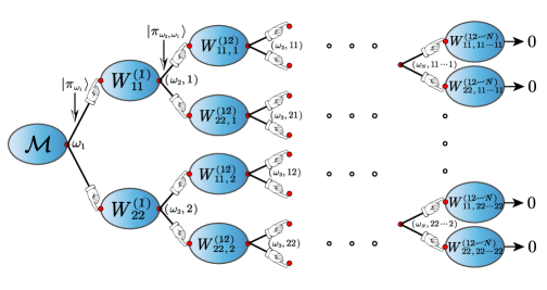
Figure 1: LMCC can be constructed through IMP using “block hollowization”, where the trace of the diagonal blocks of a matrix is transformed to zero through local unitary transformations with classical communications. The goal is to perform a full “hollowization” procedure, where all the diagonal matrix elements of the operator $\mathcal{M}$ are brought to zero. The IMP provides a feasible approach, see details in the main text and the Supplemental Material [27].

The Iterative Matrix Partition Approach to LMCC and LM.— From now on, we shall focus our discussion on pure states of $N$-qubit systems and search for optimal LM and LMCC. In this case, the measurement outcome $\omega$ in Eq. (2) becomes a string of measurement outcomes of each qubit denoted as $\omega=(\omega_{1},\,\omega_{2},\,\cdots,\,\omega_{N})$. Zhou et al [23] showed that the optimal projective LMCC can be constructed iteratively through

$$\braket{\pi_{\omega_{j},\,\omega_{1}\cdots\omega_{j-1}}^{(j)}}{M_{\omega_{1}\cdots\omega_{j-1}}^{(j)}\big{missing}}{\pi_{\omega_{j},\,\omega_{1}\cdots\omega_{j-1}}^{(j)}}=0.$$ (4)

The superscripts in basis and operators in Eq. (4) indicate the subsystems over which they are defined and

$$M_{\omega_{1}\cdots\omega_{j-1}}^{(j)}\equiv$$

$$\bra{\pi_{\omega_{1}}^{(1)}}\otimes\cdots\bra{\pi_{\omega_{j-1},\,\omega_{1}\cdots\omega_{j-2}}^{(j-1)}}\text{Tr}_{(j+1,\,\cdots N)}\mathcal{M}\ket{\pi_{\omega_{1}}^{(1)}}\otimes\cdots\ket{\pi_{\omega_{j-1},\,\omega_{1}\cdots\omega_{j-2}}^{(j-1)}}$$ (5)

is an operator defined on the $j$-th qubit with $j\geq 2$, where the subscripts in the “Tr” notation indicate the subsystems that are traced over. For $j=1$, $M^{(1)}\equiv\text{Tr}_{(2\cdots N)}\mathcal{M}$ and $\ket{\pi_{\omega_{1}}^{(1)}}$ satisfies $\braket{\pi_{\omega_{1}}^{(1)}\big{missing}}{M^{(1)}\big{missing}}{\pi_{\omega_{1}}^{(1)}}=0$. In Sec. II of the Supplemental Material [27], we show these properties naturally follow from the optimal measurement condition (2) and for optimal projective LM they reduce to

$$\braket{\pi_{\omega_{j}}^{(j)}\big{missing}}{M^{(j)}\big{missing}}{\pi_{\omega_{j}}^{(j)}}=0,$$ (6)

where $M^{(j)}\equiv\text{Tr}_{(1\cdots\cancel{j}\cdots N)}\mathcal{M},$ the subscript $\cancel{j}$ indicates that the $j$-th qubit is not traced over. A few comments in order: (i) Since $M_{\omega_{1}\cdots\omega_{j-1}}^{(j)}$ and $M^{(j)}$ are traceless, the measurement basis in Eqs. (4, 6) can be found through the “hollowization” process: A traceless matrix can be always brought to a hollow matrix, i.e., a matrix with zero diagonal entries, through unitary transformations[27, 29, 30]. (ii) While Eq. (4) is also sufficient to guarantee the optimal measurement condition (2), this is no longer true for Eq. (6).

To resolve this issue, we propose the “iterative matrix partition”(IMP) approach, which not only produces the LMCC, but also illuminates the intuition on the existence of LM. We denote the local computational basis for the $j$-th qubit as $\ket{e_{\omega_{j}}^{(j)}}$, $\omega_{j}=1,\,2$. One can compute the $\mathcal{M}$ operator in this basis (see a tutorial example in [27]). Consider

$$\mathcal{M}=\left[\begin{array}[]{c|l}M_{11}^{(\cancel{1})}&M_{12}^{(\cancel{1})}\\ \hline\cr M_{21}^{(\cancel{1})}&M_{22}^{(\cancel{1})}\end{array}\right],$$ (7)

where for fixed $\omega_{1}$ and $\mu_{1}$, $M_{\omega_{1}\mu_{1}}^{(\cancel{1})}\equiv\braket{e_{\omega_{1}}^{(1)}\big{missing}}{\mathcal{M}\big{missing}}{e_{\mu_{1}}^{(1)}}$ is a $2^{N-1}\times 2^{N-1}$ matrix that acts on all the qubits except first qubit .

Since $\mathcal{M}$ is anti-Hermitian, so is the diagonal block matrices $M_{11}^{(\cancel{1})}$ and $M_{22}^{(\cancel{1})}$. Furthermore, $\mathcal{M}$ is traceless, the trace of the two diagonal block matrices can be also brought zero through a unitary transformation on the first qubit (see Observation 3 in [27]). More precisely,

$$\mathcal{M}=\sum_{\omega_{1}\mu_{1}}W_{\omega_{1}\mu_{1}}^{(\cancel{1})}\ket{\pi_{\omega_{1}}^{(1)}}\bra{\pi_{\mu_{1}}^{(1)}}$$ (8)

where $|\pi_{\omega}^{(1)}\rangle\equiv U^{(1)}\ket{e_{\omega_{1}}^{(1)}}$, $W_{\omega_{1}\mu_{1}}^{(\cancel{1})}\equiv U^{(1)}M_{\omega_{1}\mu_{1}}^{(\cancel{1})}U^{(1)\dagger}$ and $U^{(1)\dagger}$ is chosen such that $\text{Tr}W_{11}^{(\cancel{1})}=\text{Tr}W_{22}^{(\cancel{1})}=0$. Note that $W_{11}^{(\cancel{1})}$ and $W_{22}^{(\cancel{1})}$ are also anti-Hermitian matrices.

Next, we decompose $W_{11}^{(\cancel{1})}$ and $W_{22}^{(\cancel{1})}$ in the local computational basis of the second qubit, i.e.

$$W_{\omega_{1}\omega_{1}}^{(\cancel{1})}=\sum_{\omega_{2},\,\mu_{2}}M_{\omega_{2}\mu_{2},\,\omega_{1}}^{(\cancel{12})}\ket{e_{\omega_{2}}^{(2)}}\bra{e_{\omega_{2}}^{(2)}},$$ (9)

where $M_{\omega_{2}\mu_{2},\,\omega_{1}}^{(\cancel{12})}$, analogous to $M_{\omega_{1}\mu_{1}}^{(\cancel{1})}$, is the block matrix representation of $W_{\omega_{1}\omega_{1}}^{(\cancel{1})}$ in the local computational basis of the second qubit. For fixed $\omega_{1}$, one can iterate to perform the “block-hollowization” process for $W_{\omega_{1}\omega_{1}}^{(\cancel{1})}$, leading to

$$W_{\omega_{1}\omega_{1}}^{(\cancel{1})}=\sum_{\omega_{2},\,\mu_{2}}W_{\omega_{2}\mu_{2},\,\omega_{1}}^{(\cancel{12})}\ket{\pi_{\omega_{2},\,\omega_{1}}^{(2)}}\bra{\pi_{\mu_{2},\,\omega_{1}}^{(2)}},$$ (10)

where $\ket{\pi_{\omega_{2},\,\omega_{1}}^{(2)}}\equiv U_{\omega_{1}}^{(2)}\ket{e_{\omega_{2}}^{(2)}}$ and $W_{\omega_{2}\omega_{2},\,\omega_{1}}^{(\cancel{12})}$ is traceless and anti-Hermitian for fixed $\omega_{1}$.

Iterating this process to the $N$-th qubit, we arrive at

$$W_{\omega_{N-1}\omega_{N-1},\,\omega_{1}\cdots\omega_{N-2}}^{(\cancel{1\cdots N-1})}=\sum_{\omega_{N},\,\mu_{N}}M_{\omega_{N}\mu_{N},\,\omega_{1}\cdots\omega_{N-1}}^{(\cancel{1\cdots N})}\ket{e_{\omega_{N}}^{(N)}}\bra{e_{\mu_{N}}^{(N)}},$$ (11)

where for fixed $\omega_{1},\,\cdots,\,\omega_{N-1}$, $M_{\omega_{N}\mu_{N},\,\omega_{1}\cdots\omega_{N-1}}^{(\cancel{1\cdots N})}$ is a $2\times 2$ anti-Hermitian traceless matrix. Finally, we perform the “hollowization” and obtain

$$W_{\omega_{N-1}\omega_{N-1},\,\omega_{1}\cdots\omega_{N-2}}^{(\cancel{1\cdots N-1})}$$

$$= \sum_{\omega_{N},\,\mu_{N}}W_{\omega_{N}\mu_{N},\,\omega_{1}\cdots\omega_{N-1}}^{(\cancel{1\cdots N})}\ket{\pi_{\omega_{N},\,\omega_{1}\cdots\omega_{N-1}}^{(N)}}\bra{\pi_{\mu_{N},\,\omega_{1}\cdots\omega_{N-1}}^{(N)}},$$ (12)

where $\ket{\pi_{\omega_{N},\,\omega_{1}\cdots\omega_{N-1}}^{(N)}}\equiv U_{\omega_{1}\cdots\omega_{N-1}}^{(N)}\ket{e_{\omega_{N}}^{(N)}}$ and $W_{\omega_{N}\omega_{N},\,\omega_{1}\cdots\omega_{N-1}}^{(\cancel{1\cdots N})}=0$ for $\omega_{N}=1,\,2$. The procedure is pictorially depicted in Fig. 1.

If $U_{\omega_{1}\cdots\omega_{j-1}}^{(j)}$ is independent of $\omega_{1}\cdots\omega_{j-1}$ for all $j\in[2,N]$ (the case of $j=1$ is obvious), then we call the IMP is degenerate. We prove in Sec. IV in [27] the following two observations: (i) a generic IMP gives rise to an LMCC measurement, as shown in Fig. 1. (ii) a degenerate IMP is equivalent to the existence of optimal LM.

An immediate application of the IMP approach is that it illuminates on the “self-similar” structure of the GHZ states, which guarantees the existence of local optimal measurements. Such a structure, to our best knowledge, has not been appreciated previously in the literature. To elaborate, consider the sensing Hamiltonian

$$H=\lambda S_{z},$$ (13)

and an initial GHZ state $\ket{\psi_{0}}=(|0\rangle^{\otimes N}+|1\rangle^{\otimes N})/\sqrt{2}$, where $S_{z}=\sum_{j}\sigma_{z}^{(j)}/2$ and $\ket{0},\ket{1}$ are the excited and ground states of $\sigma_{z}$, respectively. As time evolves, the state remains at a GHZ state, but with parameter-dependent relative phase, i.e., $|\psi_{\lambda}\rangle=(|0\rangle^{\otimes N}+e^{i\lambda Nt}|1\rangle^{\otimes N})/\sqrt{2}$ The $\mathcal{M}$ operator is given by

$$\mathcal{M}=\text{i}Nt(|0^{\otimes N}\rangle\langle 0^{\otimes N}|-|1^{\otimes N}\rangle\langle 1^{\otimes N}|).$$ (14)

In the first iteration, we observe that $M_{12}^{(\cancel{1})}=M_{21}^{(\cancel{1})}=0$ in the computational basis $\ket{0^{(1)}}$ and $\ket{1^{(1)}}$ vanishes, which simplifies the iteration dramatically and leads to [27]

$$U^{(1)}=\frac{1}{\sqrt{2}}\left[\begin{array}[]{cc}1&1\\ e^{i\phi^{(1)}}&-e^{i\phi^{(1)}}\end{array}\right].$$ (15)

Consequently, we immediately obtain

$$W_{\omega_{1}\omega_{1}}^{(\cancel{1})}=\frac{1}{2}(M_{11}^{(\cancel{1})}+M_{22}^{(\cancel{1})})=\frac{\text{i}Nt}{2}(|0^{\otimes N-1}\rangle\langle 0^{\otimes N-1}|-|1^{\otimes N-1}\rangle\langle 1^{\otimes N-1}|),$$ (16)

where $\omega_{1}=1,\,2$. A few observations can be drawn: (i) The first iteration of the IMP process leads to exact the same diagonal blocks $W_{11}^{(1)}=W_{22}^{(1)}$. (i) The matrix structure of $W_{\omega_{1}\omega_{1}}^{(\cancel{1})}$ , apart from the dimensionality and an irrelevant prefactor, is identical to Eq. (14) . The consequence of such a self-similar structure is that $U_{\omega_{1}}^{(2)}$, more generally $U_{\omega_{1}\cdots\omega_{k-1}}^{(k)}$, does not depend on the previous measurement outcomes. We note that $U^{(k)}$ is the the same as $U^{(1)}$ apart from the phase factor $e^{\text{i}\phi^{(k)}}.$ At the $k$-th iteration, we arrive at $W_{\omega_{k}\omega_{k}}^{(\cancel{1\cdots k})}=\text{i}Nt/2^{k}(|0^{\otimes N-k}\rangle\langle 0^{\otimes N-k}|-|1^{\otimes N-k}\rangle\langle 1^{\otimes N-k}|).$ The IMP for the GHZ state is degenerate and LMCC reduces to LM.

Fundamental Theorems on Optimal LM.— Now we present several theorems on optimal LM. Our first theorem is the following:

Theorem 1.

The qCRB of a 2-qubit pure state is universally saturated by projective LM.

Proof.

We perform the IMP procedure. After the first round, we obtain two anti-Hermitian matrix $W_{\omega_{1}\omega_{1}}^{(\cancel{1})}$ of the dimension $2\times 2$. According to Observation 2 in the Supplementary Material [27], $W_{11}^{(\cancel{1})}$ and $W_{22}^{(\cancel{1})}$ are simultaneously hollowizable. ∎

In [27], we provide a tutorial explanation demonstrating the application of the IMP approach using a two-qubit example and construct the corresponding optimal LM.

Beyond two qubits, as we will show later by a counterexample, universal saturation of the qCRB is not possible. Nevertheless, as an alternative method to the IMP approach, one can use the following theorem to determine explicitly whether an $N$-qubit pure state can saturate the qCRB.

Theorem 2.

For $N$-qubit system labeled by $\mathscr{X}_{N}=\{1,\,2,\,\cdots,N\}$, the qCRB of a pure state can be saturated by LM if and only if for each non-empty subset $\alpha\subseteq\mathscr{X}_{N}$ there exists Bloch vectors $\{\bm{n}^{(j)}\}_{j\in\alpha}$ such that

$$\text{Tr}\mathcal{M}\mathcal{N}_{\alpha}=0,\quad\mathcal{N}_{\alpha}\equiv\otimes_{n\in\alpha}\bm{n}^{(j)}\cdot\bm{\sigma}^{(j)}.$$ (17)

where the projectors of the projective LM is given by

$$\Pi_{\omega_{j}}^{(j)}=\frac{\mathbb{I}^{(j)}+(-1)^{\omega_{j}}\bm{n}^{(j)}\cdot\bm{\sigma}^{(j)}}{2},\,\omega_{j}=\pm 1.$$ (18)

Having discussed the projective LM, let us now come to generic non-projective POVM LM. For such measurements, unlike projective LM, the number of measurement basis is not necessarily bounded by two for each local spin and can become as many as the projective LMCC. Then a natural question arises: Are POVM LM more powerful than projective LM? The answer is no, according to the following theorem.

Theorem 3.

For $N$-qubit pure-state, if there is a generic qCRB-saturating POVM LM, then there must exists a qCRB-saturating projective LM.

By the virtue of Theorem 3, it suffices to focus on projective LM. If optimal projective LM cannot be found, then it is impossible to reach the qCRB by using POVM LM with a large number of measurement basis. In this sense, generic POVM LM does not help in reaching the qCRB. However, this does not exclude their other possible utilities. As we have shown before, in the projective LM basis, applying IMP to the GHZ state leads to the property of self-similarity. It is an interesting open question to search for states that display self-similarity in generic POVM LM basis, which could lead to non-GHZ-like many-body states that saturate the qCRB.

We consider a pure state $\ket{\psi_{\lambda}(t)}=U_{\lambda}(t)\ket{\psi_{0}}$ that is generated from a unitary parameter-dependent quantum channel $U_{\lambda}(t)$ and an initial pure state $\ket{\psi_{0}}$, where $U_{\lambda}(t)$ satisfied the Schrödinger equation $\text{i}\dot{U}_{\lambda}(t)=H_{\lambda}(t)U_{\lambda}(t)$. In this case, the quantum Fisher information is given by

$$I_{\lambda}=4\text{Var}\left(G_{\lambda}(t)\right){}_{\ket{\psi_{0}}},$$ (19)

and $\mathcal{M}$ can be rewritten as

$$\mathcal{M}=-2\text{i}U_{\lambda}(t)[\rho_{0},\,[G_{\lambda}(t),\,\rho_{0}]]U_{\lambda}^{\dagger}(t),$$ (20)

where the metrological generator is defined as [14, 31]

$$G_{\lambda}(t)\equiv\text{i}U_{\lambda}^{\dagger}(t)\partial_{\lambda}U_{\lambda}(t)=\int_{0}^{t}U_{\lambda}^{\dagger}(s)\partial_{\lambda}H_{\lambda}(s)U_{\lambda}(s)ds.$$ (21)

So we have the following theorem [27]:

Theorem 4.

Given a pair of initial state $\ket{\psi_{0}}$ and a unitary channel $U_{\lambda}(t)$, the qCRB of $\ket{\psi_{\lambda}(t)}$ can be saturated at the instantaneous time $t$ by LM if and only

$$\text{Cov}\left(\mathcal{N}_{\alpha}^{(\text{H})}(t)G_{\lambda}(t)\right)_{\ket{\psi_{0}}}=0,\,\forall\alpha\subseteq\mathscr{X}_{N},$$ (22)

where the set $\mathscr{X}_{N}$ is same as in Theorem 2 and $\mathcal{N}_{\alpha}^{(\text{H})}(t)\equiv U_{\lambda}^{\dagger}(t)\mathcal{N}_{\alpha}U_{\lambda}(t)$ is the Heisenberg evolution of $\mathcal{N}_{\alpha}$ and $\text{Cov}(AB)_{\ket{\psi_{0}}}\equiv\frac{1}{2}\langle\{A,\,B\}\rangle_{\ket{\psi_{0}}}-\langle A\rangle_{\ket{\psi_{0}}}\langle B\rangle_{\ket{\psi_{0}}}$.

One can check immediately that the GHZ state with $\sigma_{x}$-LM satisfies Theorem 4. Now we are in a position to give a minimum 3-qubit counter-example that fails to saturating the qCRB under LM. Consider $H_{\lambda}=\lambda H_{0},$where $H_{0}\equiv\sum_{a=x,\,y}(\sigma_{a}^{(1)}\sigma_{a}^{(2)}+\sigma_{a}^{(2)}\sigma_{a}^{(3)})$, the initial state is the W state, i.e., $|\psi_{0}\rangle=(|100\rangle+|010\rangle+|001\rangle)/\sqrt{3}$. We assume the true value of $\lambda$ is zero so that $|\psi_{\lambda}(t)\rangle=|\psi_{0}\rangle$. It should be clarified that in this case despite the state does not change over time, it does not mean the parameter cannot be estimated accurately. In fact, it is straightforward to see QFI is $4t^{2}\text{Var}[H_{0}]_{\ket{\psi_{0}}}=32t^{2}/9,$ independent of the value of $\lambda$. In [27], using symmetry arguments, we show that the set of equations determined by Eq. (22) can not be consistent with each other. Therefore, neither projective LM nor generic POVM LM exists according to Theorem 3.

Universal Approximate Saturation with Adaptive Control. — As one can see from Theorem 4, the saturation of the qCRB with LM can be very restrictive. Nevertheless, we observe that if

$$\mathcal{N}_{\alpha}^{(\text{H})}(t)\ket{\psi_{0}}\propto\ket{\psi_{0}},\,\,\forall\alpha\subseteq\mathscr{X}_{N}$$ (23)

is satisfied at time $t$, then Eq. (22) holds. Note that the case where $\ket{\psi_{0}}$ is an eigenstate of $G_{\lambda}(t)$ is trivial as it leads to a vanishing QFI.

To this end, when the initial state is a product of pure states, one can first choose $\mathcal{N}_{\alpha}(0)$ such that Eq. (23) hold at $t=0$. As time evolves, $\mathcal{N}_{\alpha}(t)$ will the spread and Eq. (23) will no longer hold. However, one can take advantage of our prior knowledge and apply a proper control Hamiltonian such that dynamics is frozen or at least very slow. That is,

$$\delta H(t)=H_{\lambda}(t)+H_{\text{1}}(t),$$ (24)

where the control Hamiltonian $H_{\text{1}}(t)=-H_{\lambda_{*}}(t)$ and $\lambda_{*}$ is our priori knowledge on the estimation parameter. Then $\mathcal{N}_{\alpha}^{(\text{H})}(t)$ remains close to $\mathcal{N}_{\alpha}(0)$ for quite long time as long as $\lambda_{*}$ is close to $\lambda$. It is worth to note that in local estimation theory, adaptive estimation is usually exploited where some refined knowledge of the estimation parameter is known a priori [32, 33, 34]. Quantum control was explored in quantum metrology before, but aiming to boosting the QFI [35, 36, 18, 31, 37] and overcome the measurement noise. [38, 39]. It is remarkable that quantum controls here, which facilities LM to saturate the qCRB is fully consistent with the QFI-boosting controls in Ref. [35, 31, 36]. Finally, we note that as long as $\lambda_{*}$ close to $\lambda$, the metrological generator associated with the dynamics generated by Eq. (24) becomes $G_{\lambda}(t)=\int_{0}^{t}\partial_{s}H_{\lambda}(s)ds$ and QFI is still given by Eq. (19). Let us consider the following an example, where

$$H_{\lambda}=\lambda S_{z}^{2},$$ (25)

and the initial state is a spin coherent state [40] parameterized by

$$|\psi_{0}\rangle=\bigotimes_{k=1}^{N}\left[\cos\frac{\theta}{2}|0\rangle^{(k)}+e^{i\phi}\sin\frac{\theta}{2}|1\rangle^{(k)}\right].$$ (26)

Equation (25) is nonlinear and non-local. It has been shown previously that precision beyond the shot-noise scaling in classical sensing [41, 14, 19] can be achieved. However, the optimal LM that reaches such a non-classical precision is still missing in the literature. To this end, we apply coherent control $H_{\text{1}}=-\lambda_{*}S_{z}^{2}$ so that $\delta H=\delta\lambda S_{z}^{2}$ where $\delta\lambda\equiv\lambda-\lambda_{*}$ state. The QFI corresponding to the initial state Eq. (26) is [27]

$$I=4t^{2}\text{Var}[S_{z}^{2}]_{\ket{\psi_{0}}}=4t^{2}\sum_{k=1}^{3}f_{k}(\cos\theta)N^{k},$$ (27)

and scales cubically in $N$, surpassing the Heisenberg limit. In Fig. 2, the comparison between the QFI and classical Fisher information (CFI) associated with the LM (18), where $\bm{n}^{(j)}=(\sin\theta\cos\phi,\,\sin\theta\sin\phi,\,\cos\theta)$ are plotted. One can readily see that qCRB is asymptotically saturated as $\lambda_{*}$ approaches $\lambda$.

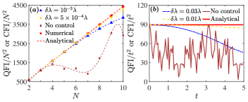
Figure 2: QFI and CFI associated with local measurements with the Hamiltonian (25) and initial state (26). The value of parameters are: $\theta=\frac{\pi}{3}$, $\phi=\frac{\pi}{2}$ and $\lambda=2$.(a) The variation of the saturation with the number of qubits $N$ for a fixed evolution time $t=1/0.01\lambda=50$. The red solid dots is the numerical calculations for the QFI while the dashed line is plotted according to Eq. (27). The blue triangles, yellow stars, and brown diamonds represent the numerically obtained CFI $/N^{2}$ under the application of different control strategies, respectively. (b) The saturation behavior of the qCRB under time-dependent evolution for $N=8$. The red solid line is plotted according to Eq.  (27), while the yellow dash-dotted line, blue dashed line, and brown solid line respectively depict the CFI under different control strategies, respectively.

Conclusion and outlook. — We systematically study optimal LMCC and LM that can saturate the qCRB in many-body sensing. We propose an IMP approach that illuminates the structure of the optimal LMCC and LM and provide several fundamental theorems on the qCRB-saturating optimal LM. We show that under LM, the qCRB can be universally saturated in an approximate way with adaptive control, regardless of the form of the sensing Hamiltonian.

Currently, in the protocols of many-body sensing [42, 43, 17, 18, 16, 14, 15], there is not yet a systematic construction of the optimal LM. Our results fill the gap between theoretical proposal of many-body sensing and its experimental realization. We expect to see their near-term implementation in noisy intermediate scale quantum devices [44, 45, 46]. Future works include generalization to qudits, continuous variable systems, and qubit-cavity systems, application to entanglement detection [47, 48, 49] and spin-squeezing [40, 50, 51], investigation of the effect of decoherence, etc.

Acknowledgement. —We thank Sisi Zhou for useful communications. JY was funded by the Wallenberg Initiative on Networks and Quantum Information (WINQ). HLS was supported by the NSFC key grants No. 12134015 and No. 92365202. SY was supported by Key-Area Research and Development Program of Guangdong Province Grant No. 2020B0303010001.

Supplemental Material

In this Supplemental Material, we present detailed discussions on (1) the optimal measurement condition, (2) properties of LMCC and LM (3) hollowization and block hollowization, (4) iterative matrix partition, (5) proofs of Theorems 2-4, (6) the three-qubit counter-example that cannot saturate the qCRB, and (7) the analytic calculations of the QFI in Eq. (27).

I Revisiting the QCRB-saturating optimal measurements

I.1 Optimal measurement condition for POVM operators

In this section, we revisit the optimal measurement condition for saturating the QCRB and find a simplified yet still necessary and sufficient condition, compared to Ref. [23]. To begin with, let us note the classical Fisher information associated with a POVM measurement is given by

$$F_{\omega}=\frac{(\text{Tr}[\partial_{\lambda}\rho_{\lambda}\Pi_{\omega}])^{2}}{\text{Tr}[\rho_{\lambda}\Pi_{\omega}]}.$$ (S1)

Following the procedure in Ref. [26], one can find that

$$F_{\omega}\leq I_{\omega},$$ (S2)

where

$$I_{\omega}=\text{Tr}[\rho_{\lambda}L\Pi_{\omega}L].$$ (S3)

The inequality is saturated provided [28]

$$\Pi_{\omega}\ket{\psi_{n\lambda}}=\xi_{\omega}\Pi_{\omega}L\ket{\psi_{n\lambda}},\,\xi_{\omega}\in\mathbb{R},\,\forall\omega,$$ (S4)

where $\ket{\psi_{n\lambda}}$ is the eigenvector of $\rho_{\lambda}$ corresponding to strictly positive eigenvalues. Summing over all the measurement outcome $\omega$ on both sides of Eq. (S2), we obtain

$$F\leq I,$$ (S5)

where

$$I\equiv\sum_{\omega}I_{\omega}\equiv\text{Tr}[\rho_{\lambda}L^{2}].$$ (S6)

Ref. [23] further recast Eq. (S4) into the following condition

$$\sqrt{\Pi_{\omega}}\mathcal{M}\sqrt{\Pi_{\omega}}=0,\,\forall\omega,$$ (S7)

if $\text{Tr}[\rho_{\lambda}\Pi_{\omega}]\neq 0$ and

$$\sqrt{\Pi_{\omega}}L\ket{\psi_{n\lambda}}=0,$$ (S8)

if $\text{Tr}[\rho_{\lambda}\Pi_{\omega}]=0$, where the POVM measurement satisfies $\sum_{\omega}\Pi_{\omega}=\mathbb{I}$.

However, we would like to point out the condition Eq. (S8) is redundant. This can be seen as follows: As shown in Ref. [28], when $\text{Tr}[\rho_{\lambda}\Pi_{\omega}]=0$ is satisfied, $\ket{\psi_{n\lambda}}$ must lies in the kernel of $\Pi_{\omega}$. As a consequence,

$$\text{Tr}[\partial_{\lambda}\rho_{\lambda}\Pi_{\omega}]=0,\qquad\text{Tr}[\Pi_{\omega}L\rho_{\lambda}]=0,\>\text{if}\>\text{Tr}[\rho_{\lambda}\Pi_{\omega}]=0.$$ (S9)

Furthermore, Eq. (S8) will also be satisfied automatically, if one substitute the expression of the SLD operator. In fact, $F_{\omega}$ should be calculated via the L’hospital rule, which turns out for that Eq. (S2) is always saturated for single-parameter estimation (see Theorem 2 in Ref. [28]). Therefore the constraint (S8) is unnecessary.

Finally, Eq. (S7) implies that

$$\Pi_{\omega}\mathcal{M}\Pi_{\omega}=0,\,\forall\omega.$$ (S10)

To prove the converse direction, one just needs to note that $\Pi_{\omega}$ and $\sqrt{\Pi}_{\omega}$ has the same support.

I.2 Rank$-1$ POVM measurements are sufficient

Now we shall prove if there exists optimal POVM measurements $\{\Pi_{\omega}\}$ that are not of rank-$1$, i.e.,

$$\Pi_{\omega}=\sum_{s}\alpha_{\omega s}\ket{\pi_{\omega s}}\bra{\pi_{\omega s}},$$ (S11)

then one can break them into rank-$1$ measurement operators $\{\Pi_{\omega s}\}$ with

$$\Pi_{\omega s}\equiv\alpha_{\omega s}\ket{\pi_{\omega s}}\bra{\pi_{\omega s}}.$$ (S12)

Since $\Pi_{\omega}$ satisfies Eq. (S4), we find

$$\sum_{s}\alpha_{\omega s}\ket{\pi_{\omega s}}\braket{\pi_{\omega s}\big{missing}}{\psi_{n\lambda}}=\xi_{\omega}\ket{\pi_{\omega s}}\braket{\pi_{\omega s}\big{missing}}{L\big{missing}}{\psi_{n\lambda}}.$$ (S13)

For fixed $\omega$, $\{\ket{\pi_{\omega s}}\}$ are orthonormal are linearly independent, we must have

$$\alpha_{\omega s}\braket{\pi_{\omega s}\big{missing}}{\psi_{n\lambda}}=\xi_{\omega}\braket{\pi_{\omega s}\big{missing}}{L\big{missing}}{\psi_{n\lambda}},$$ (S14)

which apparently leads to

$$\Pi_{\omega s}\ket{\psi_{n\lambda}}=\xi_{\omega}\Pi_{\omega s}L\ket{\psi_{n\lambda}}.$$ (S15)

This implies that $\{\Pi_{\omega s}\}$ is also an also optimal POVM measurement with rank-$1$. Note that

$$\Pi_{\omega s}\Pi_{\omega r}=\delta_{sr},$$ (S16)

but

$$\Pi_{\omega s}\Pi_{\mu r}\neq 0,\,\text{for}\,\omega\neq\mu.$$ (S17)

In summary, without loss of generality, one just need to consider rank$-1$ optimal measurements such that Eq. (2) is satisfied.

II Properties of optimal LMCC and LM

In this section, we observe useful properties of the optimal LMCC from optimal measurement condition. For LMCC, these properties in turn guarantee the optimal measurement conditions. We point out that this is the intuition and motivation that underlies the construction recipe by Zhou et al [23].

When it comes to LM, one can observe similar properties for the optimal LM from the optimal measurement condition. However, these properties alone cannot guarantee the optimal measurement condition. Thus, one needs to resort to the “bi-partition” intuition in the main text.

II.1 Properties of the optimal LMCC

We would like to find LMCC such that

$$\bra{\pi_{\omega_{1}}^{(1)}}\otimes\cdots\otimes\bra{\pi_{\omega_{1},\,\cdots\omega_{N}}^{(N)}}\mathcal{M}\ket{\pi_{\omega_{1}}^{(1)}}\otimes\cdots\otimes\ket{\pi_{\omega_{1},\,\cdots\omega_{N}}^{(N)}}=0,$$ (S18)

where

$$\sum_{\omega_{j}}\ket{\pi_{\omega_{1}\cdots\omega_{j}}^{(j)}}\bra{\pi_{\omega_{1}\cdots\omega_{j}}^{(j)}}=\mathbb{I}^{(j)},\,\forall j\in N.$$ (S19)

Interesting properties of the LMCC can be observed from the optimal measurement condition (S18).

We emphasize that the LMCC, if they exist, they must satisfy the following properties. First, we take the summation over $\omega_{2},$$\omega_{3},\cdots\omega_{N}$ in Eq. (S18) and find

$$\braket{\pi_{\omega_{1}}^{(1)}\big{missing}}{M^{(1)}\big{missing}}{\pi_{\omega_{1}}^{(1)}}=0,$$ (S20)

where

$$M^{(1)} \equiv\sum_{\omega_{2}}\cdots\sum_{\omega_{N}}\bra{\pi_{\omega_{2},\omega_{1}}^{(2)}}\otimes\cdots\otimes\bra{\pi_{\omega_{N},\omega_{1}\,\cdots\omega_{N-1}}^{(N)}}\mathcal{M}\ket{\pi_{\omega_{2},\,\omega_{1}}^{(2)}}\otimes\cdots\otimes\ket{\pi_{\omega_{N},\omega_{1}\,\cdots\omega_{N-1}}^{(N)}}$$ (S21)

$$=\text{Tr}_{(2\cdots N)}\mathcal{M}.$$ (S22)

Note that we have used Eq. (S19) and the sum must be performing in the order from $\omega_{N}$ up to $\omega_{1}$ in Eq. (S21). Given $\text{Tr}_{1}M^{(1)}=\text{Tr}\mathcal{M}=0,$it is possible to find $\ket{\pi_{\omega_{1}}^{(1)}}$ by hollowizing $M^{(1)}$ according to Sec. III.

Once $\ket{\pi_{\omega_{1}}^{(1)}}$ is found, one can use it as an input and take the summation over $\omega_{3},\cdots\omega_{N}$ in Eq. (S18) leads

$$\braket{\pi_{\omega_{2},\,\omega_{1}}^{(2)}\big{missing}}{M_{\omega_{1}}^{(2)}\big{missing}}{\pi_{\omega_{2},\omega_{1}}^{(2)}}=0,$$ (S23)

where

$$M_{\omega_{1}}^{(2)} \equiv\bra{\pi_{\omega_{1}}^{(1)}}\otimes\sum_{\omega_{3}}\cdots\sum_{\omega_{N}}\left(\bra{\pi_{\omega_{3},\,\omega_{1}\omega_{2}}^{(3)}}\otimes\cdots\otimes\bra{\pi_{\omega_{N},\,\omega_{1}\cdots\omega_{N-1}}^{(N)}}\mathcal{M}\ket{\pi_{\omega_{3},\,\omega_{1}\omega_{2}}^{(3)}}\otimes\cdots\otimes\ket{\pi_{\omega_{N},\,\omega_{1}\cdots\omega_{N-1}}^{(N)}}\right)\otimes\ket{\pi_{\omega_{1}}^{(1)}}$$

$$=\bra{\pi_{\omega_{1}}^{(1)}}\text{Tr}_{(3\dots N)}\mathcal{M}\ket{\pi_{\omega_{1}}^{(1)}}.$$ (S24)

From last step, we know

$$\text{Tr}_{2}M_{\omega_{1}}^{(2)}=\braket{\pi_{\omega_{1}}^{(1)}\big{missing}}{M^{(1)}\big{missing}}{\pi_{\omega_{1}}^{(1)}}=0.$$ (S25)

So hollowizing $M_{\omega_{1}}^{(2)}$ is also possible. In this procedure, we have the recursive relation

$$M_{\omega_{1}\cdots\omega_{j-1}}^{(j)}=\bra{\pi_{\omega_{1}}^{(1)}}\otimes\cdots\otimes\bra{\pi_{\omega_{j-1},\,\omega_{1}\cdots\omega_{j-2}}^{(j-1)}}\text{Tr}_{j+1\cdots N}\mathcal{M}\ket{\pi_{\omega_{1}}^{(1)}}\otimes\cdots\otimes\ket{\pi_{\omega_{j-1},\,\omega_{1}\cdots\omega_{j-2}}^{(j-1)}}.$$ (S26)

At the very end of the procedure, it leads to

$$\braket{\pi_{\omega_{N},\,\omega_{1}\cdots\omega_{N-1}}^{(N)}\big{missing}}{M_{\omega_{1}\cdots\omega_{N-1}}^{(N)}\big{missing}}{\pi_{\omega_{N},\,\omega_{1}\cdots\omega_{N-1}}^{(N)}}=0,$$ (S27)

where

$$M_{\omega_{1}\cdots\omega_{N-1}}^{(N)}\equiv\bra{\pi_{\omega_{1}}^{(1)}}\otimes\cdots\otimes\bra{\pi_{\omega_{N-1},\,\cdots\omega_{N-2}}^{(N-1)}}\mathcal{M}\bra{\pi_{\omega_{1}}^{(1)}}\otimes\cdots\otimes\ket{\pi_{\omega_{N-1},\,\cdots\omega_{N-2}}^{(N-1)}}.$$ (S28)

At this point, we have found the properties of the LMCC, i.e. Eqs. (S20), (S23) up to (S27), are just the consequence of Eq. (S18). It is not a prior true that they also guarantee the optimal measurement condition. However, in this case, the optimal measurement condition can be readily seen by substituting Eq. (S28) into Eq. (S27). The above analysis motivates the construction recipe by Zhou at al [23], which is listed in the following:

Step 1.0: Define $M^{(1)}\equiv\text{Tr}_{(2\cdots N)}\mathcal{M}$.

Step 1.1: Hollowizing $M^{(1)}$ leads to measurement basis $\{\ket{\pi_{\omega_{1}}}\}$ with

$$\braket{\pi_{\omega_{1}}^{(1)}}{M^{(1)}\big{missing}}{\pi_{\omega_{1}}^{(1)}}=0.$$ (S29)

Step 2.0: Use $\ket{\pi_{\omega_{1}}^{(1)}}$ as an input and define $M_{\omega_{1}}^{(2)}\equiv\text{Tr}_{(3\cdots N)}\braket{\pi_{\omega_{1}}^{(1)}}{\mathcal{M}\big{missing}}{\pi_{\omega_{1}}^{(1)}}$.

Step 2.1: Hollowizing $M^{(2)}$ leads to measurement basis $\{\ket{\pi_{\omega_{1},\,\omega_{2}}}\}$ with

$$\braket{\pi_{\omega_{1},\omega_{2}}^{(2)}}{M_{\omega_{1}}^{(2)}\big{missing}}{\pi_{\omega_{1},\,\omega_{2}}^{(2)}}=0.$$ (S30)

Step ($j$+1).0: Use $\ket{\pi_{\omega_{1}}^{(1)}},\,\cdots,\,\ket{\pi_{\omega_{1},\,\cdots\omega_{n}}^{(j)}}$as inputs and define

$$M_{\omega_{1},\,\cdots\omega_{j}}^{(j+1)} \equiv\text{Tr}_{(j+2,\,\cdots N)}\bra{\pi_{\omega_{1}}^{(1)}}\otimes\cdots\otimes\bra{\pi_{\omega_{1},\,\cdots\omega_{j}}^{(j)}}\mathcal{M}\ket{\pi_{\omega_{1}}^{(1)}}\otimes\ket{\pi_{\omega_{1},\,\cdots\omega_{j}}^{(j)}}.$$ (S31)

Remark ($j$+1).0: It is straightforward to check that $M^{(j+1)}$ is traceless.

$$\text{Tr}_{j+1}M^{(j+1)} =\text{Tr}_{(j+1,\,\cdots N)}\bra{\pi_{\omega_{1}}^{(1)}}\otimes\cdots\otimes\bra{\pi_{\omega_{j},\,\omega_{1}\cdots\omega_{j-1}}^{(j)}}\mathcal{M}\ket{\pi_{\omega_{1}}^{(1)}}\otimes\cdots\otimes\ket{\pi_{\omega_{j},\,\omega_{1}\cdots\omega_{j-1}}^{(j)}}$$

$$= \braket{\pi_{\omega_{j},\,\omega_{1}\cdots\omega_{j-1}}^{(j)}\big{missing}}{M_{\omega_{1}\cdots\omega_{j-1}}^{(j)}\big{missing}}{\pi_{\omega_{j},\,\omega_{1}\cdots\omega_{j-1}}^{(j)}}=0.$$ (S32)

II.2 Properties of LM

Similar with LMCC, the optimal measurement condition for LM is

$$\bra{\pi_{\omega_{1}}^{(1)}}\otimes\cdots\otimes\bra{\pi_{\omega_{N}}^{(N)}}\mathcal{M}\ket{\pi_{\omega_{1}}^{(1)}}\otimes\ket{\pi_{\omega_{N}}^{(N)}}=0,$$ (S33)

where

$$\sum_{\omega_{j}}\ket{\pi_{\omega_{j}}^{(j)}}\bra{\pi_{\omega_{j}}^{(j)}}=\mathbb{I}^{(j)},\,\forall j\in N.$$ (S34)

Again, if local measurements exist, they must satisfy following properties. We take the summation in Eq. (S33) except for the index $\omega_{j}$ and obtain

$$\braket{\pi_{\omega_{j}}^{(j)}\big{missing}}{M^{(j)}\big{missing}}{\pi_{\omega_{j}}^{(j)}}=0,\,\forall n,$$ (S35)

where

$$M^{(j)}=\text{Tr}_{(1\cdots\cancel{j}\cdots N)}\mathcal{M}.$$ (S36)

We note that only the first step with $j=1$ is the same as the construction for the LMCC. We emphasize the properties of the optimal measure, i.e., Eq. (S35) do not guarantee the optimal measurement condition (S33).

III The procedure of hollowization and block hollowization

As one can see from Eq. (2) in the main text, the meaning of the optimal measurements is that the $\mathcal{M}$ operator has zero-diagonal entries in the measurement basis. In this section, we present more mathematical details on the “hollowization” process discussed in the main text: A traceless matrix can be brought to zero through unitary transformations. A generalization notion of “hollowization” for block matrices, called “block hollowization” procedure is also discussed.

Proposition.

Any square traceless matrix can be transformed into a matrix with vanishing diagonal entries through a unitary similarity transformation.

The first proof of this claim, to our best knowledge, is by Fillmore [30], which is also discussed in the text book on matrix analysis [29]. An immediate corollary of above proposition is that any square matrix is unitary equivalent to a matrix with equal diagonal entries.

Just like the standard diagonalization process, it is also possible discuss simultaneous “hollowization” for multiple traceless matrices. For a $2\times 2$ Hermitian or anti-Hermitian traceless matrix, it can be parameterized by $A=\bm{a}\cdot\bm{\sigma}$ or $A=\text{i}\bm{a}\cdot\bm{\sigma}$ , where $\bm{a}$ is a real vector defined in $\mathbb{R}^{3}$. In this case, simultaneous “hollowization” process have a very clear geometrical meaning:

Observation 1.

A set of traceless $2\times 2$ Hermitian (anti-Hermitian) matrices $A_{j}=\bm{a}_{j}\cdot\bm{\sigma}$($A_{j}=\text{i}\bm{a}_{j}\cdot\bm{\sigma}$) can be simultaneously hollowized iff $\{\bm{a}_{j}\}$ are coplanar.

Proof.

We first observe that a Hermitian matrix $A=\bm{a}\cdot\bm{\sigma}$ has zero diagonal entries means they are traceless and have no $\sigma_{z}$ component, i.e., the vector $\bm{a}$ lies on the $X-Y$ plane or

$$\text{Tr}[A\sigma_{z}]=0.$$ (S37)

The backward direction can be proved as follows: If all $\bm{a}_{j}$ are on the same plane that is orthogonal to a unit normal vector $\hat{\bm{n}}$, then a rotation from $\bm{\hat{n}}$ to $+Z$-axis suffices to make the diagonal entries of all $A_{j}$ vanishing. The corresponding unitary reads

$$U_{\theta}=\exp\left\{-i\frac{\theta}{2}\frac{\bm{\hat{n}}\times\hat{\bm{z}}}{|\bm{\hat{n}}\times\hat{\bm{z}}|}\cdot\bm{\sigma}\right\},$$ (S38)

where $\theta$ is the angle between $\hat{\bm{n}}$ and $\hat{\bm{z}}$,i.e., $\cos\theta=\hat{\bm{n}}\cdot\bm{\hat{z}}$. Physically this corresponding the basis transformation. means $U_{\theta}\ket{+\bm{n}}=\ket{\uparrow}$ and $U_{\theta}\ket{-\bm{n}}=\ket{\downarrow}$. As consequence, we obtain

$$U_{\theta}\bm{n}\cdot\bm{\sigma}U_{\theta}^{\dagger}=\sigma_{z}.$$ (S39)

Using this identity, one can readily show

$$\text{Tr}(U_{\theta}A_{j}U_{\theta}^{\dagger}\sigma_{z})=\text{Tr}(A_{j}U_{\theta}^{\dagger}\sigma_{z}U_{\theta})=\text{Tr}\left((\bm{a}_{j}\cdot\bm{\sigma})(\bm{n}\cdot\bm{\sigma})\right)=\bm{a}_{j}\cdot\bm{n}=0.$$ (S40)

The forward direction can be easily seen by reversing the above argument. ∎

With Observation 1, it is clear that

Observation 2.

Two traceless $2\times 2$ Hermitian or anti-Hermitian matrices are simultaneous hollowizable.

Proof.

The proof is straightforward: two vector $\bm{a}_{1}$ and $\bm{a}_{2}$ in $\mathbb{R}^{3}$ must be coplanar. ∎

Since $\mathbb{C}^{2d}=\mathbb{C}^{2}\otimes\mathbb{C}^{d}$, one can decompose the linear transformation on $\mathbb{C}^{d}$, i.e., a $(2d)\times(2d)$ dimensional matrix $\mathcal{A}$ in the block form

$$\mathcal{A}=\left[\begin{array}[]{c|l}A_{11}&A_{12}\\ \hline\cr A_{21}&A_{22}\end{array}\right],$$ (S41)

where $A_{ij}$ is a $d\times d$ matrix acting on the linear space $\mathbb{C}^{d}$. Furthermore, if $A$ is Hermitian, then

$$A_{11}^{\dagger}=A_{11},\,A_{22}^{\dagger}=A_{11},\,A_{12}^{\dagger}=A_{21},$$ (S42)

while if $\mathcal{A}$ is anti-Hermitian,

$$A_{11}^{\dagger}=-A_{11},\,A_{22}^{\dagger}=-A_{11},\,A_{12}^{\dagger}=-A_{21}.$$ (S43)

Now we are in a position to state a theorem regarding the “block zero-trace” process:

Observation 3.

For a traceless Hermitian (anti-Hermitian) matrix $A$ decomposed into the block-structure form in Eq. (S41) can be brought to the “block hollowized” form through a unitary matrix defined on the in the auxiliary space $\mathbb{C}^{2}$, that is,$\exists$$2\times 2$ unitary matrix such that

$$U^{\dagger}\mathcal{A}U=\left[\begin{array}[]{c|l}B_{11}&B_{12}\\ \hline\cr B_{21}&B_{22}\end{array}\right],$$

with

$$\text{Tr}B_{11}=\text{Tr}B_{22}=0.$$ (S44)

Proof.

A $2\times 2$ unitary matrix can be parameterized as follows

$$U=\begin{bmatrix}\ket{+\bm{n}},\,&e^{\text{i}\beta}\ket{-\bm{n}}\end{bmatrix}=\begin{bmatrix}\cos\frac{\theta}{2}&\sin\frac{\theta}{2}e^{\text{i}\beta}\\ \sin\frac{\theta}{2}e^{i\phi}&-\cos\frac{\theta}{2}e^{\text{i}\phi+\text{i}\beta}\end{bmatrix},$$ (S45)

where

$$\ket{+\bm{n}} =\cos\frac{\theta}{2}\ket{e_{1}}+\sin\frac{\theta}{2}e^{\text{i}\phi}\ket{e_{2}},$$ (S46)

$$\ket{-\bm{n}} =\sin\frac{\theta}{2}\ket{e_{1}}-\cos\frac{\theta}{2}e^{\text{i}\phi}\ket{e_{2}},$$ (S47)

and

$$\ket{e_{1}}=\begin{bmatrix}1\\ 0\end{bmatrix},\,\ket{e_{2}}=\begin{bmatrix}0\\ 1\end{bmatrix}.$$ (S48)

Since the $U$ is also a unitary matrix on the global space $\mathbb{C}^{2}\otimes\mathbb{C}^{d}$, we expect that the trace is preserved, i.e.,

$$\text{Tr}B_{11}+\text{Tr}B_{22}=0.$$ (S49)

Therefore to satisfy Eq. (S44), it is sufficient to make the trace of one submatrix vanishes. It is straightforward calculate

$$B_{11} =\cos^{2}\frac{\theta}{2}A_{11}+\cos\frac{\theta}{2}\sin\frac{\theta}{2}(e^{\text{i}\phi}A_{12}+e^{-\text{i}\phi}A_{21})+\sin^{2}\frac{\theta}{2}A_{22},$$ (S50)

$$B_{22} =\cos^{2}\frac{\theta}{2}A_{22}-\cos\frac{\theta}{2}\sin\frac{\theta}{2}(e^{\text{i}\phi}A_{12}+e^{-\text{i}\phi}A_{21})+\sin^{2}\frac{\theta}{2}A_{11},$$ (S51)

which satisfies Eq. (S49) apparently. $\text{Tr}B_{11}=0$ leads to

$$\cos\theta\text{Tr}A_{11}+\sin\theta\text{Re}\left(e^{\text{i}\phi}\text{Tr}(A_{12})\right) =0,\>\text{if}\>\mathcal{A}=\mathcal{A}^{\dagger},$$ (S52)

$$\cos\theta\text{Tr}A_{11}+\text{i}\sin\theta\text{Im}\left(e^{\text{i}\phi}\text{Tr}(A_{12})\right) =0,\>\text{if}\>\mathcal{A}=-\mathcal{A}^{\dagger}.$$ (S53)

Thus

$$\tan\theta=\begin{cases}-\frac{\text{Tr}A_{11}}{\text{Re}\left(e^{\text{i}\phi}\text{Tr}(A_{12})\right)}&\mathcal{A}=\mathcal{A}^{\dagger}\\ \frac{\text{i}\text{Tr}A_{11}}{\text{Im}\left(e^{\text{i}\phi}\text{Tr}(A_{12})\right)}&\mathcal{A}=-\mathcal{A}^{\dagger}\end{cases},$$ (S54)

which concludes the proof. ∎

IV Proofs and examples related to the “iterative matrix partition” (IMP) approach

IV.1 Generic IMP leads to an optimal LMCC

Proof.

According to Eq. (8) in the main text, we know

$$W_{\omega_{1}\omega_{1}}^{(\cancel{1})}=\braket{\pi_{\omega_{1}}^{(1)}\big{missing}}{\mathcal{M}\big{missing}}{\pi_{\omega_{1}}^{(1)}}.$$ (S55)

Substituting this equation into Eq. (10), we obtain

$$W_{\omega_{2}\omega_{2},\,\omega_{1}}^{(\cancel{12})}=\braket{\pi_{\omega_{2},\,\omega_{1}}^{(2)}\big{missing}}{W_{\omega_{1}\omega_{1}}^{(\cancel{1})}\big{missing}}{\pi_{\omega_{2},\,\omega_{1}}^{(2)}}=\bra{\pi_{\omega_{2},\,\omega_{1}}^{(2)}}\bra{\pi_{\omega_{1}}^{(1)}}\mathcal{M}\ket{\pi_{\omega_{1}}^{(1)}}\ket{\pi_{\omega_{2},\,\omega_{1}}^{(2)}}.$$ (S56)

Iteratively, we find

$$W_{\omega_{j}\omega_{j},\,\omega_{1}\cdots\omega_{j-1}}^{(\cancel{1\cdots j})}=\bra{\pi_{\omega_{j},\,\omega_{1}\cdots\omega_{j-1}}^{(j)}}\cdots\otimes\bra{\pi_{\omega_{2},\,\omega_{1}}^{(2)}}\otimes\bra{\pi_{\omega_{1}}^{(1)}}\mathcal{M}\ket{\pi_{\omega_{1}}^{(1)}}\otimes\ket{\pi_{\omega_{2},\,\omega_{1}}^{(2)}}\otimes\cdots\ket{\pi_{\omega_{j},\,\omega_{1}\cdots\omega_{j-1}}^{(j)}}.$$ (S57)

Continuing to the last step, according to Eq. (12), we obtain

$$W_{\omega_{N}\omega_{N},\,\omega_{1}\cdots\omega_{N-1}}^{(\cancel{1\cdots N})}=\braket{\pi_{\omega_{N},\,\omega_{1}\cdots\omega_{N-1}}^{(N)}\big{missing}}{W_{\omega_{N-1}\omega_{N-1},\,\omega_{1}\cdots\omega_{N-2}}^{(\cancel{1\cdots N-1})}\big{missing}}{\pi_{\omega_{N},\,\omega_{1}\cdots\omega_{N-1}}^{(N)}}.$$ (S58)

Substituting Eq. (S57) into Eq. (S58), we arrive at

$$W_{\omega_{N}\omega_{N},\,\omega_{1}\cdots\omega_{N-1}}^{(\cancel{1\cdots N})}=\bra{\pi_{\omega_{N},\,\omega_{1}\cdots\omega_{N-1}}^{(N)}}\cdots\otimes\bra{\pi_{\omega_{2},\,\omega_{1}}^{(2)}}\otimes\bra{\pi_{\omega_{1}}^{(1)}}\mathcal{M}\ket{\pi_{\omega_{1}}^{(1)}}\otimes\ket{\pi_{\omega_{2},\,\omega_{1}}^{(2)}}\otimes\cdots\ket{\pi_{\omega_{N},\,\omega_{1}\cdots\omega_{N-1}}^{(N)}}.$$ (S59)

Upon noticing that $W_{\omega_{N}\omega_{N},\,\omega_{1}\cdots\omega_{N-1}}^{(\cancel{1\cdots N})}=0$ for all $(\omega_{1},\cdots,\omega_{N})$, the proof is completed ∎

IV.2 A degenerate IMP leads to an optimal LM

Proof.

The proof is straightforward based on the proof in Sec. IV.1. Since for degenerate IMP $U_{\omega_{j},\,\omega_{1}\cdots\omega_{j-1}}$ is independent of $\omega_{1},\,\cdots,\,\omega_{j-1}$ for all $j\in[1,N]$, $\ket{\pi_{\omega_{j},\,\omega_{1}\cdots\omega_{j-1}}^{(j)}}\equiv U_{\omega_{j},\,\omega_{1}\cdots\omega_{j-1}}\ket{e_{\omega_{j}}^{(j)}}$ is therefore also independent of $\omega_{1},\,\cdots,\,\omega_{j-1}$. So Eq. (S59) becomes

$$W_{\omega_{N}\omega_{N}}^{(\cancel{1\cdots N})}=\bra{\pi_{\omega_{1}}^{(1)}}\otimes\bra{\pi_{\omega_{2}}^{(2)}}\otimes\cdots\bra{\pi_{\omega_{N}}^{(N)}}\mathcal{M}\ket{\pi_{\omega_{1}}^{(1)}}\otimes\ket{\pi_{\omega_{2}}^{(2)}}\otimes\cdots\ket{\pi_{\omega_{N}}^{(N)}},$$ (S60)

that is $\mathcal{M}$ is hollowized with projective LM basis. ∎

IV.3 An optimal LM allows a degenerate IMP

Proof.

Given the optimal measurement condition for LM, Eq. (S33), we construct

$$U^{(j)}=\sum_{\omega_{j}}\ket{\pi_{\omega_{j}}^{(j)}}\bra{e_{\omega_{j}}^{(j)}}.$$ (S61)

It is then straightforward to check that the application of $U^{(1)}$ on the first qubit leads to

$$W_{\omega_{1}\omega_{1}}^{(\cancel{1})}=\braket{\pi_{\omega_{1}}^{(1)}\big{missing}}{\mathcal{M}\big{missing}}{\pi_{\omega_{1}}^{(1)}}.$$ (S62)

According to Eq. (S33), we find

$$\text{Tr}_{(2\cdots N)}W_{\omega_{1}\omega_{1}}^{(\cancel{1})}=\sum_{\omega_{2},\,\cdots\omega_{N}}\bra{\pi_{\omega_{2}}^{(1)}}\otimes\cdots\otimes\bra{\pi_{\omega_{N}}^{(N)}}W_{\omega_{1}\omega_{1}}^{(\cancel{1})}\ket{\pi_{\omega_{2}}^{(1)}}\otimes\ket{\pi_{\omega_{N}}^{(N)}}=0.$$ (S63)

Next, we apply $U^{(2)}$on the second qubit, leading to

$$W_{\omega_{2}\omega_{2},\,\omega_{1}}^{(\cancel{12})}=\braket{\pi_{\omega_{2}}^{(2)}\big{missing}}{W_{\omega_{1}\omega_{1}}^{(\cancel{1})}\big{missing}}{\pi_{\omega_{2}}^{(2)}}.$$ (S64)

Similarly with Eq. (S63), one can easily show

$$\text{Tr}_{(3\cdots N)}W_{\omega_{2}\omega_{2},\,\omega_{1}}^{(\cancel{12})}=0.$$ (S65)

With mathematical induction, one can prove that

$$W_{\omega_{j}\omega_{j},\,\omega_{j-1}\cdots\omega_{1}}^{(\cancel{1\cdots j})}=\bra{\pi_{\omega_{j}}^{(j)}}\cdots\otimes\bra{\pi_{\omega_{2}}^{(2)}}\otimes\bra{\pi_{\omega_{1}}^{(1)}}\mathcal{M}\ket{\pi_{\omega_{1}}^{(1)}}\otimes\ket{\pi_{\omega_{2}}^{(2)}}\otimes\cdots\ket{\pi_{\omega_{j}}^{(j)}},$$ (S66)

with

$$\text{Tr}W_{\omega_{j}\omega_{j},\,,\,\omega_{j-1}\cdots\omega_{1}}^{(\cancel{1\cdots j})}=0,\,\forall j.$$ (S67)

∎

IV.4 A two-qubit tutorial example for the “iterative matrix partition” approach

Let us now illustrate IMP approach with the two-qubit pure state

$$\left|\psi_{\lambda}\right\rangle=\cos\beta|01\rangle+\sin\beta e^{i\lambda}|10\rangle.$$ (S68)

where $\beta$ is a parameter independent of $\lambda$. It can be readily calculated that

$$\mathcal{M}=\text{i}\sin 2\beta(|01\rangle\langle 01|-|10\rangle\langle 10|)-\text{i}\cos 2\beta(e^{i\lambda}|10\rangle\langle 01|+e^{-i\lambda}|01\rangle\langle 10|).$$ (S69)

In the first step of the IMP, according to Sec. III in the Supplemental Material [27], we choose

$$U^{(1)}=\frac{1}{\sqrt{2}}\left[\begin{array}[]{cc}1&1\\ e^{i\phi}&-e^{i\phi}\end{array}\right]\text{, }$$ (S70)

where the phase $e^{i\phi}$ is arbitrary , leading to

$$\begin{array}[]{l}W_{11}^{(\cancel{1})}=\frac{i}{2}\left[\begin{array}[]{cc}-\sin 2\beta&-\cos 2\beta e^{i(\lambda-\phi)}\\ -\cos 2\beta e^{i(\phi-\lambda)}&\sin 2\beta\end{array}\right],\\ W_{22}^{(\cancel{1})}=\frac{i}{2}\left[\begin{array}[]{cc}-\sin 2\beta&\cos 2\beta e^{i(\lambda-\phi)}\\ \cos 2\beta e^{i(\phi-\lambda)}&\sin 2\beta\end{array}\right].\end{array}$$ (S71)

Next, a unitary matrix $U^{(2)}$ which is independent of $\omega_{1}$

$$U^{(2)}=\frac{1}{\sqrt{2}}\left[\begin{array}[]{cc}1&-e^{i\left(\lambda-\phi-\frac{\pi}{2}\right)}\\ e^{-i\left(\lambda-\phi-\frac{\pi}{2}\right)}&1\end{array}\right]\text{. }$$ (S72)

The comparison between QFI and CFI corresponding to the LM basis forming the local unitary transformations Eqs. (S70, S72) are depicted in Figure S1, which confirms universality of the saturation of the qCRB for 2-qubit pure states.

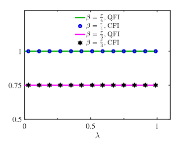
Figure S1: The ratio between CFI and QFI as functions of parameter $\lambda$ for the example of two-qubit state given by Eq. (S68). The CFI is computed from the LM basis found by the IMP approach while the QFI is computed according to Eq. (1).

V Proof of Theorem 2

Proof.

The projectors of a projective measurement on the $j$-th qubit is parameterized by

$$\Pi_{\omega_{j}}^{(j)}=\frac{\mathbb{I}^{(j)}+(-1)^{\omega_{j}}\bm{n}\cdot\bm{\sigma}}{2},\;\omega_{j}=\pm 1.$$ (S73)

It is straightforward to calculate

$$\prod_{j}\Pi_{\omega_{j}}^{(j)} =\frac{1}{2^{N}}\left(\mathbb{I}^{(1)}+(-1)^{\omega_{1}}\bm{n}^{(1)}\cdot\bm{\sigma}^{(1)}\right)\otimes\left(\mathbb{I}^{(2)}+(-1)^{\omega_{2}}\bm{n}^{(2)}\cdot\bm{\sigma}^{(2)}\right)\otimes\cdots\left(\mathbb{I}^{(N)}+(-1)^{\omega_{N}}\bm{n}^{(N)}\cdot\bm{\sigma}^{(N)}\right)$$

$$=\frac{1}{2^{N}}\left(\mathbb{I}+\sum_{\alpha\subseteq\mathscr{X},\,\alpha\neq\emptyset}(-1)^{\sum_{j\in\alpha}\omega_{j}}\otimes_{j\in\alpha}n^{(j)}\cdot\bm{\sigma}^{(j)}\right).$$ (S74)

Upon defining

$$\mathcal{N}_{\alpha}=\otimes_{j\in\alpha}n^{(j)}\cdot\bm{\sigma}^{(j)},$$ (S75)

the optimal measurement condition (S33) is equivalent to

$$\sum_{\alpha\subseteq\mathscr{X}_{N},\,|\alpha|\geq 1}(-1)^{\sum_{j\in\alpha}\omega_{j}}\text{Tr}(\mathcal{M}\mathcal{N}_{\alpha})=0,$$ (S76)

where $|\alpha|$ denotes the cardinality of the set $\alpha$ and we have used the fact that $\text{Tr}\mathcal{M}=0$. Apparently, Eq. (17) in Theorem 2 is sufficient for Eq. (S76) to hold. We prove the converse in several steps as follows:

Step 1: Let us first observe, upon setting $\omega_{N}=1$ and $\omega_{N}=-1$, respectively, while keeping all the remaining $\omega_{j}$’s fixed, we find

$$\sum_{\alpha\subseteq\mathscr{X}_{N}\backslash\{N\},\,|\alpha|\geq 1}(-1)^{\sum_{j\in\alpha}\omega_{j}}\text{Tr}(\mathcal{M}\mathcal{N}_{\alpha})+\sum_{\beta\cup\{N\},\,\beta\subseteq\mathscr{X}_{N}\backslash\{N\},\,|\beta|\geq 1}(-1)^{\sum_{j\in\beta}\omega_{j}}\text{Tr}(\mathcal{M}\mathcal{N}_{\beta\cup\{N\}}) =0,\,\omega_{N}=1,$$ (S77)

$$\sum_{\alpha\subseteq\mathscr{X}_{N}\backslash\{N\},\,|\alpha|\geq 1}(-1)^{\sum_{j\in\alpha}\omega_{j}}\text{Tr}(\mathcal{M}\mathcal{N}_{\alpha})-\sum_{\beta\cup\{N\},\,\beta\subseteq\mathscr{X}_{N}\backslash\{N\},\,|\beta|\geq 1}(-1)^{\sum_{j\in\beta}\omega_{j}}\text{Tr}(\mathcal{M}\mathcal{N}_{\beta\cup\{N\}}) =0,\,\omega_{N}=-1.$$ (S78)

Summing over these two equations, we find

$$\sum_{\alpha\subseteq\mathscr{X}_{N}\backslash\{N\},\,|\alpha|\geq 1}(-1)^{\sum_{j\in\alpha}\omega_{j}}\text{Tr}(\mathcal{M}\mathcal{N}_{\alpha})=0.$$ (S79)

Iterating above procedure, we find

$$\sum_{\alpha\subseteq\mathscr{X}_{N}\backslash\{N,\,N-1,\,\cdots 2\},\,|\alpha|\geq 0}(-1)^{\sum_{j\in\alpha}\omega_{j}}\text{Tr}(\mathcal{M}\mathcal{N}_{\alpha})=0,$$ (S80)

i.e.,

$$\text{Tr}(\mathcal{M}\mathcal{N}_{1})=0.$$ (S81)

In a similar manner, one can show

$$\text{Tr}(\mathcal{M}\mathcal{N}_{\alpha})=0,\,|\alpha|=1.$$ (S82)

Step 2: Substituting Eq. (S82) into Eq. (S76), we find

$$\sum_{\alpha\subseteq\mathscr{X}_{N},\,|\alpha|\geq 2}(-1)^{\sum_{j\in\alpha}\omega_{j}}\text{Tr}(\mathcal{M}\mathcal{N}_{\alpha})=0.$$ (S83)

Following similar manipulation in Step 1, one can first choose some $\omega_{j}$ and set it to be $+1$ and $-1$, respectively whiling keeping the remaining ones fixed. Then summing over the two equation corresponding to $\omega_{j}=\pm 1$, the index $j$ is then removing from equation, leading to

$$\sum_{\alpha\subseteq\mathscr{X}_{N}\backslash\{j\},\,|\alpha|\geq 2}(-1)^{\sum_{j\in\alpha}\omega_{j}}\text{Tr}(\mathcal{M}\mathcal{N}_{\alpha})=0.$$ (S84)

Iterating this process, we find

$$\text{Tr}(\mathcal{M}\mathcal{N}_{\alpha})=0,\,|\alpha|=2.$$ (S85)

Now one can clearly tell, when we arrive at Step $N$, we will arrive at

$$\text{Tr}(\mathcal{M}\mathcal{N}_{\alpha})=0,\;|\alpha|=N,$$ (S86)

which concludes the proof. ∎

VI Proof of Theorem 3

Proof.

For the $j$-th qubit, the most general rank-$1$ measurement can be parameterized as follows:

$$\tilde{\Pi}_{\omega_{j}}^{(j)}=x_{\omega_{j}}\ket{+\bm{n}_{\omega_{j}}^{(j)}}\bra{+\bm{n}_{\omega_{j}}^{(j)}}=\frac{x_{\omega_{j}}}{2}\left(\mathbb{I}^{(j)}+\bm{n}_{\omega_{j}}^{(j)}\cdot\bm{\sigma}^{(j)}\right),$$ (S87)

where $x_{\omega_{j}}\in(0,\,1]$ and the normalization condition

$$\sum_{\omega_{j}}\tilde{\Pi}_{\omega_{j}}^{(j)}=\mathbb{I}^{(j)},$$ (S88)

leads to

$$\sum_{\omega_{j}}x_{\omega_{j}}^{(j)}=2,\quad\sum_{\omega_{j}}x_{\omega_{j}}\bm{n}_{\omega_{j}}^{(j)}=0.$$ (S89)

According to the qCRB-saturating condition (S7), we find

$$\text{Tr}\left(\mathcal{M}\otimes_{j}\tilde{\Pi}_{\omega_{j}}^{(j)}\right)=0,$$ (S90)

which can be simplified as

$$\text{Tr}\left(\mathcal{M}\otimes_{j}(\ket{+\bm{n}_{\omega_{j}}^{(j)}}\bra{+\bm{n}_{\omega_{j}}^{(j)}})\right)=\text{Tr}\left(\mathcal{M}\otimes_{j}\frac{\mathbb{I}^{(j)}+\bm{n}_{\omega_{j}}^{(j)}\cdot\bm{\sigma}^{(j)}}{2}\right)=0.$$ (S91)

Without loss of generality, one can assuming $\omega_{j}=1,\,2,\cdots,\,d_{j}$. For $j$-th qubit we set $\omega_{j}=1$ and by summing over all the remaining $\omega$’s find,

$$\text{Tr}\left(\mathcal{M}\ket{+\bm{n}_{1}^{(j)}}\bra{+\bm{n}_{1}^{(j)}}\right)=\frac{1}{2}\text{Tr}\left(\mathcal{M}(\mathbb{I}^{(j)}+\bm{n}_{1}^{(j)}\cdot\bm{\sigma}^{(j)})\right)=0,$$ (S92)

which reduces to

$$\text{Tr}\left(\mathcal{M}\mathcal{N}_{\alpha}\right)=0,$$ (S93)

where $\alpha=\{j\}$ and $\mathcal{N}_{\alpha}$ is defined as in Eq. (S75) with $\bm{n}^{(j)}$ identified as $\bm{n}_{1}^{(j)}$. Similarly, by considering two qubits $j,k$, we obtain

$$\text{Tr}\left(\mathcal{M}\frac{(\mathbb{I}^{(j)}+\bm{n}_{1}^{(j)}\cdot\bm{\sigma}^{(j)})(\mathbb{I}^{(k)}+\bm{n}_{1}^{(k)}\cdot\bm{\sigma}^{(k)})}{2}\right)=0,$$ (S94)

which leads to Eq. (S93) with $\alpha=\{j,\,k\}$. In a similar manner, by induction,

$$\text{Tr}(\mathcal{M}\mathcal{N}_{\alpha})=0,\quad\forall\alpha\subseteq\mathscr{X}_{N}.$$ (S95)

∎

VII Proof of Theorem 4

Proof.

For simplicity, we shall suppress the time-dependence of $U_{\lambda}$ on $t$. For unitary channels and pure initial states, i.e.,

$$\rho_{\lambda}=U_{\lambda}\rho_{0}U_{\lambda}^{\dagger},$$ (S96)

with $\rho_{0}=\ket{\psi_{0}}\bra{\psi_{0}}$, it is straightforward to compute

$$\partial_{\lambda}\rho_{\lambda}=\partial_{\lambda}U_{\lambda}\rho_{0}U_{\lambda}^{\dagger}+U_{\lambda}\rho_{0}\partial_{\lambda}U_{\lambda}^{\dagger}=-\text{i}U_{\lambda}[G_{\lambda},\,\rho_{0}]U_{\lambda}^{\dagger}.$$ (S97)

Thus we find

$$\mathcal{M}=2[\rho_{\lambda},\,\partial_{\lambda}\rho_{\lambda}]=-2\text{i}U_{\lambda}[\rho_{0},\,[G_{\lambda},\,\rho_{0}]]U_{\lambda}^{\dagger}.$$ (S98)

In the special case of $U_{\lambda}=e^{-\text{i}H_{0}t\lambda}$, $G_{\lambda}=tH_{0}$, $M$ takes a simple form

$$\mathcal{M}=-2\text{i}tU_{\lambda}[\rho_{0},\,[H_{0},\,\rho_{0}]]U_{\lambda}^{\dagger}.$$ (S99)

Alternatively, in terms of $\rho_{\lambda}$

$$\mathcal{M}=2\text{i}t\left(\left\{H_{0}\text{,}\,\rho_{\lambda}\right\}-2\langle\psi_{0}|H_{0}|\psi_{0}\rangle\rho_{\lambda}\right),$$ (S100)

Substituting Eq. (S98) into Eq. (17), we arrive at

$$\text{Tr}\left([\rho_{0},\,[G_{\lambda},\,\rho_{0}]]\mathcal{N}_{\alpha}^{(\text{H})}\right)=0,$$ (S101)

Eq. (S101) can be rewritten as

$$\text{Tr}\left([G_{\lambda},\,\rho_{0}][\mathcal{N}_{\alpha}^{(\text{H})},\,\rho_{0}]\right)=0.$$ (S102)

leads to Eq. (22) in the main text. ∎

VIII Details on the three-qubit counter-example

Let us first note the symmetries in the initial states. We denote the computational basis

$$\ket{e_{1}}=\ket{001},\,\ket{e_{2}}=\ket{010},\,\ket{e_{3}}=\ket{001},$$ (S103)

$$\mathcal{V}_{o}=\text{span}\{\ket{e_{\alpha}}\}_{\alpha=1}^{3},$$ (S104)

and the orthogonal complement of $\mathcal{V}_{o}$ as $\mathcal{V}_{o}^{\perp}$. Clearly, $\mathcal{V}_{o}$ is the odd parity subspace with one ”$\ket{1}$” state. We observe that when acting on computational basis, $\sigma_{x}^{(j)}$ and $\sigma_{y}^{(j)}$ flip the computational basis for the $j$-th qubit while $\sigma_{z}^{(j)}$ left the computational basis unchanged, that is

$$\sigma_{a}^{(j)}|e_{\alpha}\rangle\in\mathcal{V}_{o}^{\perp},\>\forall\alpha=1,\,2,\,3,\,a=x,\,y.$$ (S105)

$$\sigma_{a}^{(j)}\sigma_{b}^{(k)}\sigma_{c}^{(l)}|e_{\alpha}\rangle\in\mathcal{V}_{o}^{\perp},\,\forall\alpha=1,\,2,\,3,\,a,\,b,\,c=x,\,y.$$ (S106)

More generally, for an operator $\mathcal{O}$ of odd parity, i.e., a combination of Pauli operators, flips the states at odd number of times,

$$\mathcal{O}|e_{\alpha}\rangle\in\mathcal{V}_{o}^{\perp},\>\forall\alpha=1,\,2,\,3,$$ (S107)

Furthermore, even for operators with even parity, we note that

$$\sigma_{a}^{(1)}\sigma_{b}^{(2)}\ket{001}\in\mathcal{V}_{o}^{\perp},\,\sigma_{a}^{(2)}\sigma_{b}^{(3)}\ket{100}\in\mathcal{V}_{o}^{\perp},\,\text{etc},\,a=x,\,y.$$ (S108)

Next, we note that initial states $\ket{\psi_{0}}$ also possesses permutation symmetry of spins, as well as $U(1)$ symmetry, i.e.,

$$\sum_{j}\sigma_{z}^{(j)}\ket{\psi_{0}}=\ket{\psi_{0}}.$$ (S109)

The parity, permutation and $U(1)$ symmetries will simplify our subsequent calculations dramatically.

Now we are in a position to list the all the equations in Eq. (22). When $\lambda=0$, $G_{\lambda}(t)=tH_{0}$, where

$$H_{0}=\sigma_{x}^{(1)}\sigma_{x}^{(2)}+\sigma_{x}^{(2)}\sigma_{x}^{(3)}+\sigma_{y}^{(1)}\sigma_{y}^{(2)}+\sigma_{y}^{(2)}\sigma_{y}^{(3)},$$ (S110)

and

$$\mathcal{N}_{\alpha}^{(\text{H})}(t)=\mathcal{N}_{\alpha}(0).$$ (S111)

So Eq. (22) becomes

$$\text{Cov}\left(\mathcal{N}_{\alpha}(0)H_{0}\right)_{\ket{\psi_{0}}}=0.$$ (S112)

First, taking $\alpha=\{j\}$ with $j\in\{1,2,3\}$, we find

$$\braket{\psi_{0}\big{missing}}{\left(\bm{n}^{(j)}\cdot\bm{\sigma}^{(j)}\right)H_{0}\big{missing}}{\psi_{0}}-\langle\psi_{0}|H_{0}|\psi_{0}\rangle n_{z}^{(j)}=0.$$ (S113)

With Eq. (S107), the above equation reduces to

$$n_{z}^{(j)}\left(\braket{\psi_{0}\big{missing}}{\sigma_{z}^{(j)}H_{0}\big{missing}}{\psi_{0}}-\langle\psi_{0}|H_{0}|\psi_{0}\rangle\right)=0.$$ (S114)

Using Eq. (S108) and the permutation symmetry of $\ket{\psi_{0}}$,

$$\braket{\psi_{0}\big{missing}}{\sigma_{a}^{(j)}\sigma_{a}^{(k)}\big{missing}}{\psi_{0}} =\braket{\psi_{0}\big{missing}}{\sigma_{a}^{(1)}\sigma_{a}^{(2)}\big{missing}}{\psi_{0}}$$

$$=\frac{1}{3}\left(\braket{010\big{missing}}{\sigma_{a}^{(1)}\sigma_{a}^{(2)}\big{missing}}{100}+\braket{100\big{missing}}{\sigma_{a}^{(1)}\sigma_{a}^{(2)}\big{missing}}{010}\right)$$

$$=\frac{2}{3},\;a=x,\,y.$$ (S115)

Since $\sigma_{z}^{(3)}\ket{e_{\alpha}}\in\mathcal{V}_{o}$ with $\alpha=1,\,2,\,3$, we conclude

$$\braket{\psi_{0}\big{missing}}{\sigma_{z}^{(3)}\sigma_{a}^{(1)}\sigma_{a}^{(2)}\big{missing}}{\psi_{0}}=\braket{\psi_{0}\big{missing}}{\sigma_{a}^{(1)}\sigma_{a}^{(2)}\big{missing}}{\psi_{0}}=\frac{2}{3}.$$ (S116)

Then according to the permutation symmetry and $U(1)$ symmetry (S109), we conclude

$$\braket{\psi_{0}\big{missing}}{\sigma_{z}^{(1)}\sigma_{a}^{(1)}\sigma_{a}^{(2)}\big{missing}}{\psi_{0}}=\braket{\psi_{0}\big{missing}}{\sigma_{z}^{(2)}\sigma_{a}^{(1)}\sigma_{a}^{(2)}\big{missing}}{\psi_{0}}=0.$$ (S117)

In summary,

$$\braket{\psi_{0}\big{missing}}{\sigma_{z}^{(l)}\sigma_{a}^{(j)}\sigma_{a}^{(k)}\big{missing}}{\psi_{0}}=\begin{cases}\frac{2}{3}&j\neq k\neq l\neq j\\ 0&l=j\>\text{or}\>l=k\end{cases},$$ (S118)

which also implies

$$\braket{\psi_{0}\big{missing}}{\sigma_{x}^{(j)}\sigma_{y}^{(k)}\big{missing}}{\psi_{0}}=0,\,j\neq k.$$ (S119)

According to Eq. (S115), we conclude

$$\langle\psi_{0}|H_{0}|\psi_{0}\rangle=\frac{8}{3},$$ (S120)

and according to Eq. (S118)

$$\braket{\psi_{0}\big{missing}}{\sigma_{z}^{(j)}H_{0}\big{missing}}{\psi_{0}}=\begin{cases}\frac{4}{3}&j=1,\,3\\ 0&j=2\end{cases}.$$ (S121)

Therefore we obtain $n_{z}^{(j)}=0$. Consequently, we can parameterize as

$$\bm{n}^{(j)}\cdot\bm{\sigma}^{(j)}=\cos\beta^{(j)}\sigma_{x}^{(j)}+\sin\beta^{(j)}\sigma_{y}^{(j)}.$$ (S122)

Combing this parameterization with parity symmetry, we find for $\alpha=\{1,\,2,3\}$, Eq. (S112) is satisfied automatically thanks to the parity symmetry. Next we take $\alpha=\{k,\,l\}$ in Eq. (S112) with $k\neq l,\,k,\,l\in\{1,2,3\}$, we find

$$\braket{\psi_{0}\big{missing}}{\left(\bm{n}^{(k)}\cdot\bm{\sigma}^{(k)}\otimes\bm{n}^{(l)}\cdot\bm{\sigma}^{(l)}\right)H_{0}\big{missing}}{\psi_{0}}-\braket{\psi_{0}\big{missing}}{\bm{n}^{(k)}\cdot\bm{\sigma}^{(k)}\otimes\bm{n}^{(l)}\cdot\bm{\sigma}^{(l)}\big{missing}}{\psi_{0}}\langle\psi_{0}|H_{0}|\psi_{0}\rangle=0,$$ (S123)

which implies,

$$\cos\left(\beta^{(k)}-\beta^{(l)}\right)=0.$$ (S124)

for any pair of $(k,\,l)$, which is impossible.

IX Analytical calculations of Eq.  (27)

Define a $N$-qubit highest-weight state $|j,\,j\rangle\equiv|0^{\otimes N}\rangle$ with $j=N/2$ such that $S_{z}|j,\,j\rangle=j|j,\,j\rangle$ and $S_{+}|j,\,j\rangle=0$. Then

$$\left(S_{-}\right)^{p}|j,\,j\rangle=\sqrt{\frac{N!p!}{(N-p)!}}|j,\,j-p\rangle,\quad p=0,1,\ldots,N$$ (S125)

where $|j,\,j-p\rangle$ is the eigenstate of $S_{z}$ such that $S_{z}|j,\,j-p\rangle=(\frac{N}{2}-p)|j,\,j-p\rangle$.

The spin coherent state Eq. (26) can be equivalently expressed as [40]

$$|\psi_{0}\rangle=\frac{\exp\left(\mu S_{-}\right)}{\left(1+|\mu|^{2}\right)^{\frac{N}{2}}}|j,\,j\rangle=\frac{1}{\left(1+|\mu|^{2}\right)^{\frac{N}{2}}}\sum_{p=0}^{N}\sqrt{\frac{N!}{p!(N-p)!}}\mu^{p}|j,\,j-p\rangle,\quad\mu=\tan\left(\frac{\theta}{2}\right)e^{i\phi},\>\theta\in[0,\pi),\phi\in[0,2\pi).$$ (S126)

Define the generating function

$$F(\beta) \equiv\langle\psi_{0}|e^{\text{i}S_{z}\beta}|\psi_{0}\rangle=\left(1+|\mu|^{2}\right)^{-N}e^{\text{i}\beta N/2}\sum_{p=0}^{N}\left(\frac{(N)!}{p!(N-p)!}\right)\left(\left|\mu\right|^{2}e^{-\text{i}\beta}\right)^{p}$$

$$=\frac{\left(e^{\text{i}\beta/2}+\left|\mu\right|^{2}e^{-\text{i}\beta/2}\right)^{N}}{\left(1+\left|\mu\right|^{2}\right)^{N}},$$ (S127)

where in the last step we have used $\sum_{p=0}^{N}\frac{(N)!}{p!(N-p)!}\left|\mu\right|^{2p}=\left(1+\left|\mu\right|^{2}\right)^{N}$. We note

$$\text{Var}[S_{z}^{2}]_{\ket{\psi_{0}}}=\left\langle\psi_{0}\left|S_{z}^{4}\right|\psi_{0}\right\rangle-\left(\left\langle\psi_{0}\left|S_{z}^{2}\right|\psi_{0}\right\rangle\right)^{2}=\left[\frac{\partial^{4}F(\beta)}{\partial\beta^{4}}-\left(\frac{\partial^{2}F(\beta)}{\partial\beta^{2}}\right)^{2}\right]\bigg{|}_{\beta=0}.$$ (S128)

Carrying out the derivatives, we obtain

$$\text{Var}[S_{z}^{2}]_{\ket{\psi_{0}}}= \left(-\frac{3}{8}(1-\cos\theta)^{4}+\frac{3}{2}(1-\cos\theta)^{3}-\frac{7}{4}(1-\cos\theta)^{2}+\frac{1}{2}(1-\cos\theta)\right)N$$ (S129)

$$+\left(\frac{5}{8}(1-\cos\theta)^{4}-\frac{5}{2}(1-\cos\theta)^{3}+3(1-\cos\theta)^{2}+\cos\theta-1\right)N^{2}$$

$$+\left(-\frac{1}{4}(1-\cos\theta)^{4}+(1-\cos\theta)^{3}-\frac{5}{4}(1-\cos\theta)^{2}+\frac{1}{2}(1-\cos\theta)\right)N^{3}.$$

One can immediate read off the expression for $f_{k}(\cos\theta)$ from above equation.

References

Peskin and Schroeder [2015]M. E. Peskin and D. V. Schroeder, An Introduction To
Quantum Field Theory, Student Economy Edition, 1st ed. (Westview Press, 2015).
Huang [2010]K. Huang, Quantum Field Theory:
From Operators to Path Integrals, 2nd Edition, 2nd ed. (Wiley-VCH, Weinheim, 2010).
Riedel et al. [2010]M. F. Riedel, P. Böhi,
Y. Li, T. W. Hänsch, A. Sinatra, and P. Treutlein, Nature 464, 1170 (2010).
Hyllus et al. [2012]P. Hyllus, W. Laskowski,
R. Krischek, C. Schwemmer, W. Wieczorek, H. Weinfurter, L. Pezzé, and A. Smerzi, Physical Review A 85, 022321 (2012).