Linear stability of the elliptic relative equilibria for the restricted $N$-body problem: two special cases

Abstract

In this paper, we consider the elliptic relative equilibria of the restricted $N$-body problems, where the $N-1$ primaries form an Euler-Moulton collinear central configuration or a $(1+n)$-gon central configuration. We obtain the symplectic reduction to the general restricted $N$-body problem. For the first case, by analyzing the relationship between this restricted $N$-body problems and the elliptic Lagrangian solutions, we obtain the linear stability of the restricted $N$-body problem by the ${\omega}$-Maslov index. Via numerical computations, we also obtain conditions of the stability on the mass parameters under $N=4$ and the symmetry of the central configuration. For the second case, there exist three positions $S_{1},S_{2}$ and $S_{3}$ of the massless body (up to rotations of angle $\frac{2\pi}{n}$). For ${m_{0}\over m}$ sufficiently large, we show that the elliptic relative equilibria is linearly unstable if the eccentricity $0\leq e<e_{0}$ and the massless body lies at $S_{1}$ or $S_{2}$; while the elliptic relative equilibria is linear stability if the massless body lies at $S_{3}$.

Keywords: restricted $N$-body problem, elliptic Euler-Moulton central configuration, reduction, linear stability.

AMS Subject Classification: 70F10, 70H14, 34C25.

1 Introduction and main results

In the classical planar $N$-body problems of celestial mechanics, the position vectors of the $N$-particles are denoted by $q_{1},\dots,{q_{N}}\in{\bf R}^{2}$, and the masses are represented by $m_{1},\dots,{m_{N}}>0$. By Newton’s second law and the law of universal gravitation, the system of equations is

$$m_{i}\ddot{q_{i}}=\frac{\partial U}{\partial q_{i}},\quad i=1,{\dots,N},$$ (1.1)

where $U(q)=U(q_{1},{\dots,q_{N}})=\sum_{1\leq i<j\leq{N}}\frac{m_{i}m_{j}}{|q_{i}-q_{j}|}$ is the potential function and $|\cdot|$ is the standard norm of vector in ${\bf R}^{2}$. Suppose the configuration space is

$$\hat{\chi}:=\left\{q=(q_{1},{\dots,q_{N}})\in({\bf R}^{2})^{{N}}\;|\sum_{i=1}^{{N}}m_{i}q_{i}=0,q_{i}\neq q_{j},\forall i\neq j\right\}.$$

For the period $T$, the corresponding action functional is

$$\mathbf{A}(q)=\int_{0}^{T}\left[\sum_{i=1}^{{N}}\frac{m_{i}|\dot{q}_{i}(t)|^{2}}{2}+U(q(t))\right]{\mathrm{d}}t,$$ (1.2)

which is defined on the loop space $W^{1,2}({\bf R}/T{\bf Z},\hat{\chi})$. The periodic solutions of (1.1) correspond to critical points of the action functional (1.2). Let $p_{1},{\dots,p_{N}}\in{\bf R}^{2}$ be the momentum vectors of the particles respectively. It is well-known that (1.1) can be reformulated as a Hamiltonian system by

$$\dot{p}_{i}=-\frac{\partial H}{\partial q_{i}},\;\dot{q}_{i}=\frac{\partial H}{\partial p_{i}},\quad\mbox{for}\;i=1,{\dots,N},$$ (1.3)

with the Hamiltonian function

$$H(p,q)=\sum_{i=1}^{{N}}\frac{|p_{i}|^{2}}{2m_{i}}-U(q_{1},{\dots,q_{N}}).$$ (1.4)

One special class of periodic solutions to the planar $N$-body problem is the elliptic relative equilibrium (ERE for short) [20]. It is generated by a central configuration and the Keplerian motion. A central configuration (C.C. for short) is formed by $N$ position vectors $\left(q_{1},\ldots,q_{N}\right)=\left(a_{1},\ldots,a_{N}\right)$ which satisfy

$$-\lambda m_{i}q_{i}=\frac{\partial U}{\partial q_{i}},\forall\;1\leq i\leq N,$$ (1.5)

where $\lambda=U(a)/{I(a)}>0$ and $I(a)={\sum_{i=1}^{N}}m_{i}|a_{i}|^{2}$ is the moment of inertia. A planar central configuration of the $N$-body problem gives rise to a solution of (1.1) where each particle moves on a specific Keplerian orbit while the totality of the particles move according to a homothetic motion.

The linear stability of the ERE is determined by the eigenvalues of the linearized Poincaré map. Let ${\bf U}$ denote the unit circle in the complex plane. The ERE is spectrally stable if all eigenvalues of linearized Poincaré map are on ${\bf U}$; it is linearly stable if Poincaré map is semi-simple and spectrally stable; it is linearly unstable if at least one pair of eigenvalues are not on ${\bf U}$. Since the nineteenth century [22], the researches on the stability have always been active in celestial mechanics because it reveals the dynamics near the period orbits. However, it has always been one difficult task to obtain the linear stability of ERE, because the linearized Hamiltonian systems are non-autonomous, especially when for the elliptic orbits. Many results on linear stability of the three-body problems have been obtained over the past decades by numerical methods [16, 17, 18], bifurcation theory [21] and the index theory [6, 4, 7, 24]. To the best of our knowledge, the ${\omega}$-Maslov index theory is the only analytical method to obtain the full picture of the stability and instability to the ERE, such as the elliptic Lagrangian solution [6, 4, 7], and the elliptic Euler solution [24, 25].

When it comes to $N$-body problems when $N\geq 4$, the research on stability of ERE is quite active in the past decades. One well-studied case is the elliptic rhombus solution [15, 11, 12] which are linearly unstable. For the restricted $4$-body problem with three primaries forming Lagrangian equilateral configuration, the full bifurcation diagram of the stability and instability has been obtained for all possible masses and all eccentricity [13, 10]. Furthermore, one stable region of the linear stability has been found. Regarding the linear stability of other ERE to the four-body problem, readers may refer to [23, 5]

In this paper, we focus on the restricted $N$-body problem with the primaries forming an Euller-Moulton collinear central configuration (see [25]) or a $(1+n)$-gon central configuration (see [19, 5]). It is reasonable to study the stability problem of the massless particle. since the “massless body” can be imaged as a space station and the massive bodies form a planetary system.

We first apply the symplectic reduction method [20] to the general restricted $N$-body problem. Let $P$ denote the inertial position of the massless body zero, which moves in the gravitational field of the $N-1$ primaries, without disturbing their motion. The corresponding Hamiltonian function for this $N$th body is given by

$$H(P,q,t)=\frac{1}{2}|P|^{2}-\sum_{i=1}^{N-1}\frac{m_{i}}{|r(t)R({\theta}(t))a_{i}-q|}.$$ (1.6)

Here $r=r(\theta(t))$ is the Kepler elliptic orbit given through the true anomaly ${\theta}={\theta}(t)$by

$$r({\theta}(t))=\frac{p}{1+e\cos{\theta}(t)},$$ (1.7)

where $p=a(1-e^{2})$ and $a>0$ is the latus rectum of the ellipse (1.7). By Proposition 2.1, the ERE $(P(t),q(t))^{T}$ of the system (1.3) is in time $t$ where $q(t)=r(t)R(\theta(t))a_{N}$ and $P(t)=\dot{q}(t)$. It can be transformed to the new solution $(\bar{Z}(\theta),\bar{z}(\theta))^{T}=(0,\sigma,\sigma,0)^{T}$ in the true anomaly $\theta$ as the new variable for the original Hamiltonian function $H$ given by (2.2). We then have the reduced Hamiltonian system is given in the theorem.

Theorem 1.1.

The linearized Hamiltonian system of (2.2) at the ERE $\zeta_{0}\equiv(\bar{Z}(\theta),\bar{z}(\theta))^{T}=(0,\sigma,\sigma,0)^{T}\in{\bf R}^{4}$ depending on the true anomaly $\theta$ is given by

$$\dot{\xi}(\theta)=JB(\theta)\xi(\theta),$$ (1.8)

with

$$B(\theta)=H^{\prime\prime}(\theta,\bar{Z},\bar{z})|_{\bar{\xi}=\xi_{0}}=\left(\begin{array}[]{cccc|cccc}I_{2}&-J_{2}\\ J_{2}&I_{2}-\frac{1}{1+e\cos{\theta}}D\end{array}\right),$$ (1.11)

where

$$D=I_{2}-\frac{1}{\mu}\left(\sum_{i=1}^{N-1}\frac{m_{i}}{|a_{i}-a_{N}|^{3}}\right)I+\frac{3}{\mu}\sum_{i=1}^{N-1}m_{i}\frac{(a_{i}-a_{N})(a_{i}-a_{N})^{T}}{|a_{i}-a_{N}|^{5}}.$$ (1.12)

The corresponding quadratic Hamiltonian function is given by

$$H_{2}(\theta,\bar{Z},\bar{z})=\frac{1}{2}|\bar{Z}|^{2}+\bar{Z}\cdot J\bar{z}+\frac{1}{2}\left(I_{2}-\frac{D}{1+e\cos{\theta}}\right)|\bar{z}|^{2}.$$ (1.13)

Since $D$ depends on the central configuration, it is difficult to compute $D$ for a general central configuration. That’s why we turn our attention to two special problems.

The first special problem is when the primaries form an Euler-Moulton collinear configuration and the $N$ bodies span ${\bf R}^{2}$. Denote the eigenvalues of $D$ by ${\lambda}_{3}$ and ${\lambda}_{4}$. By Proposition 3.1, we have that both ${\lambda}_{3}$ and ${\lambda}_{4}$ are positive and ${\lambda}_{3}+{\lambda}_{4}=3$. By this property, we show the relationship between the Maslov index of $\xi_{{\alpha},e}$ given by (1.8) and the Maslov index of ${\gamma}_{\beta,e}$ which is the elliptic Lagrangian solutions in [4].

Since the elliptic Lagrangian solutions have already been well-studied in [4], by the properties of the Maslov index, we define three curves ${\beta}_{s}(e)$, ${\beta}_{s}(e)$ and ${\beta}_{k}(e)$ from left to right in $({\beta},e)\in[0,9]\times[0,1)$ according to the $\omega$-Maslov indices of $\xi_{{\beta},e}$. By the ${\omega}$-Maslov index theory [14], we obtain the normal forms of $\xi_{{\beta},e}(2\pi)$ and then the linear stability as follows.

Theorem 1.2.

1. We have $\xi_{\beta,e}(2\pi)\approx R\left(\theta_{1}\right)\diamond R\left(\theta_{2}\right)$ for some $\theta_{1}$ and $\theta_{2}\in(\pi,2\pi)$, and thus it is strongly linearly stable on the segment $0<\beta<\beta_{s}(e)$;

2. We have $\left.\xi_{\beta,e}(2\pi)\approx D(\lambda)\diamond R(\theta)\right)$ for some $0>\lambda\neq-1$ and $\theta\in(\pi,2\pi)$ and it is elliptic-hyperbolic, and thus linearly unstable on the segment $\beta_{s}(e)<\beta<\beta_{m}(e)$.

3. We have $\xi_{\beta,e}(2\pi)\approx R\left(\theta_{1}\right)\diamond R\left(\theta_{2}\right)$ for some $\theta_{1}\in(0,\pi)$ and $\theta_{2}\in(\pi,2\pi)$ with $2\pi-\theta_{2}<\theta_{1}$, and thus it is strongly linearly stable on the segment $\beta_{m}(e)<\beta<\beta_{k}(e)$.

Note that it is also possible that ${\beta}_{s}(e)={\beta}_{m}(e)$, or ${\beta}_{m}(e)={\beta}_{k}(e)$ for some $e$ in $[0,1)$. For these cases, the corresponding normal forms of $\xi_{{\beta},e}$ are given in Theorem 3.3.

For the circular case and $N=4$, we first numerically relationships between ${\beta}$ and $m_{1}$, $m_{2}$, $m_{3}$. Since $m_{1}+m_{2}+m_{3}=1$, we can plot the stable regions with respect to in $m_{1}$ and $m_{2}$ by definition of ${\beta}$ in (3.1), (3.2) and Theorem 1.2. We show these results in (a) of Figure 1.

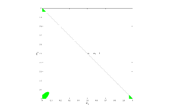
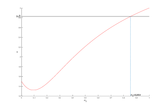
(a) The linear stability of circular solution.	(b) The symmetric case.

Figure 1: In Figure (a), the shade regions in the $(m_{1},m_{3})$-plane show the all the possible choices of $(m_{1},m_{2},m_{3})=(m_{1},1-m_{1}-m_{3},m_{3})$ of the circular orbit such that the system is linear stable. The Figure (b) shows the changes of $\alpha$ with respect to $m_{2}$ in the symmetric case

If we further assume that $m_{1}=m_{3}$. We have the following numerical results shown in (b) of Figure 1.

Theorem 1.3.

If $e=0$ and $m_{1}=m_{3}$, $\xi_{{\beta},e}$ is linear stable for $m_{2}\in(0.854,1)$.

The second special problem is when the primaries form a $(1+n)$-gon central configuration.

Suppose $n$ equal masses placed at the vertices of a regular polygon and rotating about $m_{0}$ at its center. Here note that $n=N-2$. In [1], D. Bang and B.Elmabsout find the positions of relative equilibrium for the massless body lie (up to rotations of angle $\frac{2\pi}{n}$) on the semi-axes ${\theta}=0$ and ${\theta}=\frac{\pi}{n}$ (see Figure 2):

(i) On the semi-axis ${\theta}=0$, there are two solutions $\rho=S_{1}>1$, and $\rho=S_{2},0<S_{2}<1$;

(ii) On the semi-axis ${\theta}=\frac{\pi}{n}$, there is one solution $\rho=S_{3}>1$.

Here, $S_{1},S_{2}$ and $S_{3}$ also denote the positions of the massless body, respectively. In the same paper, D. Bang and B.Elmabsout have proved that $S_{1}$ and $S_{2}$ are spectrally unstable for every $m_{0}>0$, while $S_{3}$ is linearly stable for $n\geq 7$ if $\frac{m_{0}}{m}$ is sufficiently large. Their analysis based on the methods which analytically compute means of functions on regular $n$-gons and study cyclic quantities of the complex variables in [2]. However, they just consider the circular orbits, i.e., the eccentricity $e=0$.

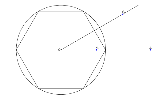
Figure 2: Positions of relative equilibrium for the massless body in the case $m_{0}>0$.

For the elliptic relative equilibrium with eccentricity $e\in[0,1)$, we have

Theorem 1.4.

If the massless body lies at $S_{1}$ or $S_{2}$, there exist $e_{0}\in(0,1)$ such that, the elliptic relative equilibrium is linearly unstable when ${m_{0}\over M}$ is sufficiently large and the eccentricity $e\in[0,e_{0}]$.

Theorem 1.5.

If the massless body lies at $S_{3}$, the elliptic relative equilibrium is linear stability when ${m_{0}\over M}$ is sufficiently large.

This paper is organized as follows. We first introduce the generalized symplectic reduction method to the restricted $N$-body problem in Section 2. We then use the ${\omega}$-Maslov index theory to obtain the linear stability of the restricted $N$-body problem when the primaries form an Euler-Muoulton central configuration in Section 3. We also consider the symmetric case by assuming $m_{1}=m_{3}$ of the restricted $4$-body problem in Section 3. In Section 4, we study the linear stability problem when the primaries form an $(1+n)$-gon central configuration. Theorem 1.4 and Theorem 1.5 are also proved there.

2 Reduction for the restricted $N$-body problem

The central configuration coordinates for a class of periodic solutions of the $n$-body problem was introduced [20]. In this section, we generalize this reduction to the restricted $N$-body problem. For the given masses $m=(m_{1},m_{2},\ldots,m_{N-1})\in({\bf R}^{+})^{N-1}$ of $N-1$ primaries let $a=(a_{1},a_{2},\ldots,a_{N-1})$ be an $(N-1)$-body central configuration of $m$ satisfying $m_{1}+m_{2}+\ldots+m_{N-1}=1$. Using normalization $2I(a)=\sum_{i=1}^{N-1}m_{i}|a_{i}|^{2}=1$ and assuming $\mu=U(a)=\sum_{1\leq i<j\leq N-1}\frac{m_{i}m_{j}}{|a_{i}-a_{j}|}$, we have

$$\sum_{j=1,j\neq i}^{N-1}\frac{m_{j}(a_{j}-a_{i})}{|a_{j}-a_{i}|^{3}}=-\frac{U(a)}{2I(a)}a_{i}=-\mu a_{i}.$$ (2.1)

Proposition 2.1.

There exists a symplectic coordinate change $\xi=(P,q)^{T}\;\mapsto\;\bar{\xi}=(\bar{Z},\bar{z})^{T},$ such that using the true anomaly ${\theta}$ as the variable the resulting Hamiltonian function of the $n$-body problem is given by

$$H(\theta,\bar{Z},\bar{z})=\frac{1}{2}|\bar{Z}|^{2}+\bar{z}\cdot J\bar{Z}+\frac{p-r}{2p}|\bar{z}|^{2}-\frac{r}{{\sigma}}\sum_{i=1}^{N-1}{m_{i}\over|{\sigma}a_{i}-\bar{z}|},$$ (2.2)

where $J=(\begin{smallmatrix}0&-1\\ 1&0\end{smallmatrix})$, $r({\theta})=\frac{p}{1+e\cos{\theta}}$, $\mu$ defined by (2.1), ${\sigma}=(\mu p)^{1/4}$ and $p$ is given in (1.7).

Proof.

Inspired by Lemma 3.1 of [20], we carry the coordinate changes in four steps.

Step 1. Rotating coordinates via the matrix $R({\theta}(t))$ in time $t$.

We change first the coordinates $\xi$ to $\hat{\xi}=(\hat{Z},\hat{z})^{T}\in({\bf R}^{2})^{2}$ which rotates with the speed of the true anomaly. The transformation matrix is given by the rotation matrix $R({\theta})=(\begin{smallmatrix}\cos{\theta}&-\sin{\theta}\\ \sin{\theta}&\cos{\theta}\end{smallmatrix})$. The generating function of this transformation is given by

$$\hat{F}(t,P,\hat{z})=-P\cdot R({\theta})\hat{z},$$ (2.3)

and for $1\leq i\leq n-1$ the transformation is given by

$$q=-\frac{\partial\hat{F}}{\partial P}=R({\theta})\hat{z},\quad\hat{Z}=-\frac{\partial\hat{F}}{\partial\hat{z}}=R({\theta})^{T}P,.$$ (2.4)

Writing $\dot{R}({\theta}(t))=\frac{d}{dt}R({\theta}(t))$, and noting that $R({\theta})^{T}=R({\theta})^{-1}$ and $\dot{R}({\theta})=\dot{{\theta}}JR({\theta})$ we obtain the function

$$\hat{F}_{t}\equiv\frac{\partial\hat{F}}{\partial t}=-P\cdot\dot{R}({\theta})\hat{z}=-\hat{Z}\cdot R({\theta})^{T}\dot{R}({\theta})\hat{z}=-\dot{{\theta}}\left(\hat{Z}\cdot R({\theta})^{T}JR({\theta})\hat{z}\right)=\dot{{\theta}}(\hat{z}\cdot J\hat{Z}).$$ (2.5)

Because ${\theta}={\theta}(t)$ depends on $t$, by adding the function $\frac{\partial\hat{F}}{\partial t}$ to the Hamiltonian function $H$ in (1.6), as in Line 5 in p.272 of [20], we obtain the Hamiltonian function $\hat{H}$ in the new coordinates:

$$\hat{H}(t,\hat{Z},\hat{z})=H_{0}(P,q)+\hat{F}_{t}=\frac{1}{2}|\hat{Z}|^{2}+(\hat{z}\cdot J\hat{Z})\dot{{\theta}}-\sum_{i=1}^{N-1}{m_{i}\over|r(t)a_{i}-\hat{z}|},$$ (2.6)

where the variables of $H_{0}$ are functions of ${\theta}$, $\hat{Z}$, $\hat{z}$, given by (2.4).

Step 2. Dilating coordinates via the polar radius $r=|z(t)|$.

We change the coordinates $\hat{\xi}$ to $\tilde{\xi}=(\tilde{Z},\tilde{z})$ which dilate with $r=|z(t)|$ given by (1.7). The position coordinates are transformed by $\hat{z}=r\tilde{z}$. It is natural to scale the momenta by $1/r$ to get $\hat{Z}=\tilde{Z}/r$. But it turns out that the new transformation

$$\hat{Z}=\frac{1}{r}\tilde{Z}+\dot{r}\tilde{z}$$ (2.7)

makes the resulting Hamiltonian function simpler. This transformation is generated by the function

$$\tilde{F}(t,\tilde{Z},\hat{z})=\frac{1}{r}\tilde{Z}\cdot\hat{z}+\frac{\dot{r}}{2r}|\hat{z}|^{2},$$ (2.8)

and is given by

$$\tilde{z}=\frac{\partial\tilde{F}}{\partial\tilde{Z}}=\frac{1}{r}\hat{z},\hat{Z}=\frac{\partial\tilde{F}}{\partial\hat{z}}=\frac{1}{r}\tilde{Z}+\frac{\dot{r}}{r}\hat{z}=\frac{1}{r}\tilde{Z}+\dot{r}\tilde{z},$$

with

$$\frac{\partial\tilde{F}}{\partial t}=-\frac{\dot{r}}{r^{2}}\tilde{Z}\cdot\hat{z}+\frac{\ddot{r}r-\dot{r}^{2}}{2r^{2}}|\hat{z}|^{2}=-\frac{\dot{r}}{r}\tilde{Z}\cdot\tilde{z}+\frac{\ddot{r}r-\dot{r}^{2}}{2}|\tilde{z}|^{2},$$ (2.9)

by (2.7).

In this case, as in the last two lines on p.272 of [20], the Hamiltonian function $\hat{H}$ in (2.6) becomes the new Hamiltonian function $\tilde{H}$ in the new coordinates:

$$\tilde{H}(t,\tilde{Z},\tilde{z}) \equiv \hat{H}(t,\hat{Z},\hat{z})+\tilde{F}_{t}$$ (2.10)

$$= \frac{1}{2r^{2}}|\tilde{Z}|^{2}+\frac{\dot{r}}{r}\tilde{Z}\cdot\tilde{z}+\frac{\dot{r}^{2}}{2}(|\tilde{z}|^{2})+(\tilde{z}\cdot J\tilde{Z})\dot{{\theta}}-\sum_{i=1}^{N-1}{m_{i}\over|r(t)a_{i}-r(t)\tilde{z}|}+\tilde{F}_{t}$$

$$= \frac{1}{2r^{2}}|\tilde{Z}|^{2}+\frac{r\ddot{r}}{2}|\tilde{z}|^{2}+(\tilde{z}\cdot J\tilde{Z})\dot{{\theta}}-\frac{1}{r}\sum_{i=1}^{N-1}{m_{i}\over|a_{i}-\tilde{z}|}.$$

Step 3. Coordinates via the true anomaly ${\theta}$ as the independent variable.

Here we use the true anomaly ${\theta}\in[0,2\pi]$ as an independent variable instead of $t\in[0,T]$ to simplify the study. This is achieved by dividing the Hamiltonian function $\tilde{H}$ in (2.10) by $\dot{{\theta}}$. Assuming $\dot{{\theta}}(t)>0$ for all $t\in[0,T]$ and $\tilde{\xi}\in W^{1,2}({\bf R}/(T{\bf Z}),{\bf R}^{8})$ we consider the action functional corresponding to the Hamiltonian system:

$$f(\tilde{\xi}) = \int_{0}^{T}(\frac{1}{2}\dot{\tilde{\xi}}(t)\cdot J\tilde{\xi}(t)-\tilde{H}(t,\tilde{\xi}(t)))dt$$

$$= \int_{0}^{2\pi}\left(\frac{1}{2}\frac{\dot{\tilde{\xi}}(t({\theta}))}{\dot{{\theta}}(t)}\cdot J\tilde{\xi}(t)-\frac{\tilde{H}(t,\tilde{\xi}(t({\theta})))}{\dot{{\theta}}(t)}\right)d{\theta}$$

$$= \int_{0}^{2\pi}\left(\frac{1}{2}\tilde{\xi}^{\prime}({\theta})\cdot J\tilde{\xi}({\theta})-\tilde{H}({\theta},\tilde{\xi}({\theta}))\right)d{\theta}.$$

Here we used $\tilde{\xi}^{\prime}({\theta})$ to denote the derivative of $\tilde{\xi}({\theta})$ with respect to ${\theta}$. But in the following we shall still write $\dot{\tilde{\xi}}({\theta})$ for the derivative with respect to ${\theta}$ instead of $\tilde{\xi}^{\prime}({\theta})$ for notational simplicity.

Note that the elliptic Kepler orbit (1.7) satisfies $r(t)^{2}\dot{{\theta}}(t)=\sqrt{\mu p}=\sqrt{\mu a(1-e^{2})}={\sigma}^{2}$ with ${\sigma}=(\mu p)^{1/4}.$ Note that $a=\mu^{1/3}(T/2\pi)^{2/3}$ with $T$ being the minimal period of the orbit (1.7), we have

$${\sigma}=(\mu a(1-e^{2}))^{1/4}=\mu^{1/3}(\frac{T}{2\pi})^{1/6}(1-e^{2})^{1/4}\;\in\;(0,\mu^{1/3}(\frac{T}{2\pi})^{1/6}]$$

depending on $e$, when the mass $\mu$ and the period $T$ are fixed. Note that similarly we have $p={\sigma}^{4}/\mu$ depends on $e$ too. Note that the function $r$ satisfies

$$\ddot{r}=\frac{\mu p}{r^{3}}-\frac{\mu}{r^{2}}=\mu\left(\frac{p}{r^{3}}-\frac{1}{r^{2}}\right).$$

Therefore we get the Hamiltonian function $\tilde{H}$ in the new coordinates:

$$\tilde{H}({\theta},\tilde{Z},\tilde{z}) \equiv \frac{1}{\dot{{\theta}}}\tilde{H}(t,\tilde{Z},\tilde{z})$$ (2.11)

$$= \frac{1}{2r^{2}(t)\dot{{\theta}}(t)}|\tilde{Z}|^{2}+\frac{r(t)\ddot{r}(t)}{2\dot{{\theta}}(t)}|\tilde{z}|^{2}+\tilde{z}\cdot J\tilde{Z}-\frac{1}{r(t)\dot{{\theta}}(t)}\sum_{i=1}^{N-1}{m_{i}\over|a_{i}-\tilde{z}|}$$

$$= \frac{1}{2{\sigma}^{2}}|\tilde{Z}|^{2}+\tilde{z}\cdot J\tilde{Z}+\frac{\mu(p-r({\theta}))}{2{\sigma}^{2}}|\tilde{z}|^{2}-\frac{r({\theta})}{{\sigma}^{2}}\sum_{i=1}^{N-1}{m_{i}\over|a_{i}-\tilde{z}|},$$

where $r({\theta})=p/(1+e\cos{\theta})$. Note that now the minimal period $T$ of the elliptic solution $\tilde{z}=\tilde{z}({\theta})$ becomes $2\pi$ in the new coordinates in terms of true anomaly ${\theta}$ as an independent variable.

Step 4. Coordinates via the dilation of ${\sigma}=(p\mu)^{1/4}$.

The last transformation is the dilation $(\tilde{Z},\tilde{z})\;=\;({\sigma}\bar{Z},{\sigma}^{-1}\bar{z})$. This transformation is symplectic and independent of the true anomaly ${\theta}$. Thus the Hamiltonian function $\tilde{H}$ in (2.11) becomes a new Hamiltonian function:

$$H({\theta},\bar{Z},\bar{z})\equiv\tilde{H}({\theta},{\sigma}\bar{Z},{\sigma}^{-1}\bar{z})=\frac{1}{2}|\bar{Z}|^{2}+\bar{z}\cdot J\bar{Z}+\frac{p-r}{2p}|\bar{z}|^{2}-\frac{r}{{\sigma}}\sum_{i=1}^{N-1}{m_{i}\over|{\sigma}a_{i}-\bar{z}|}.$$ (2.12)

The proof is complete. ∎

Suppose that $(P(t),q(t))^{T}$ is the solution of system (1.3) with $q(t)=r(t)R(\theta(t))a_{N}$, and $P(t)=\dot{q}(t).$ By Proposition 2.1, it is transformed to the new solution $(\bar{Z}(\theta),\bar{z}(\theta))^{T}$ in the true anomaly $\theta$ as the new variable for the original Hamiltonian function $H$ of (1.6), which is given by

$$\bar{Z}(\theta)=(0,\sigma)^{T}\qquad\bar{z}(\theta)=(\sigma,0)^{T}$$ (2.13)

Therefore, we can prove the Theorem 1.1 directly.

Proof of Theorem 1.1.

In this proof we omit all the upper bars on the variables of $H$ in (2.2). By (2.2), we have

$$H_{z}=JZ+\frac{p-r}{p}z-\frac{r}{\sigma}{\partial\over\partial z}\left(\sum_{i=1}^{N-1}{m_{i}\over|{\sigma}a_{i}-\bar{z}|}\right)|_{z={\sigma}a_{N}},\quad H_{Z}=Z-Jz,$$ (2.14)

and

$$H_{ZZ}=I,\quad H_{Zz}=-J,\quad H_{zZ}=J,\quad H_{zz}=\frac{p-r}{p}I-\frac{r}{\sigma}{\partial^{2}\over\partial z^{2}}\left(\sum_{i=1}^{N-1}{m_{i}\over|{\sigma}a_{i}-\bar{z}|}\right)|_{z={\sigma}a_{N}},$$ (2.15)

where all the items above are $2\times 2$ matrices, and we denote by $H_{x}$ and $H_{xy}$ the derivative of $H$ with respect to $x$, and the second derivative of $H$ with respect to $x$ and then $y$ respectively for $x$ and $y\in{\bf R}$.

Now evaluating the corresponding functions at the special solution $({0,{\sigma}},{{\sigma},0})^{T}\in{\bf R}^{4}$ of (2.13) with $z=({\sigma},0)^{T}$, and summing them up, we obtain

$$\frac{\partial^{2}}{\partial z^{2}}\left(\sum_{i=1}^{N-1}{m_{i}\over|{\sigma}a_{i}-\bar{z}|}\right)\Bigg{|}_{\xi_{0}} = -\left(-\sum_{i=1}^{N-1}{m_{i}\over|\sigma a_{i}-z|^{3}}\right)I+3\sum_{i=1}^{N-1}m_{i}\frac{({\sigma}a_{i}-z)({\sigma}a_{i}-z)^{T}}{|\sigma a_{i}-z|^{5}}$$ (2.16)

$$= -{1\over{\sigma}^{3}}\left(\sum_{i=1}^{N-1}{m_{i}\over|a_{i}-a_{N}|^{3}}\right)I+{3\over{\sigma}^{3}}\sum_{i=1}^{N-1}m_{i}\frac{(a_{i}-a_{N})(a_{i}-a_{N})^{T}}{|a_{i}-a_{N}|^{5}}.$$

Hence, we have

$$H_{zz} = I_{2}-{r\over p}I_{2}-{r\over p}{{\sigma}^{3}\over\mu}\left[-{1\over{\sigma}^{3}}\left(\sum_{i=1}^{N-1}{m_{i}\over|a_{i}-a_{N}|^{3}}\right)I+{3\over{\sigma}^{3}}\sum_{i=1}^{N-1}m_{i}\frac{(a_{i}-a_{N+1})(a_{i}-a_{N})^{T}}{|a_{i}-a_{N}|^{5}}\right]$$ (2.17)

$$= I_{2}-{r\over p}\left[I_{2}-{1\over\mu}\left(\sum_{i=1}^{N-1}{m_{i}\over|a_{i}-a_{N}|^{3}}\right)I+{3\over\mu}\sum_{i=1}^{N-1}m_{i}\frac{(a_{i}-a_{N})(a_{i}-a_{N})^{T}}{|a_{i}-a_{N}|^{5}}\right],$$

where the last equality of the first formula follows from the definition of $\mu$ in (2.1). Thus the proof is complete. ∎

3 When the primaries form an Euler-Moulton central configuration

We now consider the linear stability of special relative equilibrium in the $N$ body problem with one small mass away form the line of the $N-1$ primaries which form an Euler-Moulton central configuration. A typical example is the ERE orbit of the restricted $4$-bodies, the Sun, the Earth, the Moon and one space station. By the analytical results, we compute the one special case which is $m_{1}=m_{3}$ numerically for $N=4$ in Section 3.2.

3.1 Analytical results on the linear stability

Proposition 3.1.

Suppose that $a_{i}$ for $1\leq i\leq N-1$ forms an Euler collinear configuration and $a_{i}$ for $1\leq i\leq N$ span ${\bf R}^{2}$. The eigenvalues ${\lambda}_{3}$ and ${\lambda}_{4}$ of $D$ defined by (1.12) are both positive and satisfy

$${\lambda}_{3}+{\lambda}_{4}=3.$$ (3.1)

Proof.

By (1.12) and the direct computations, we have that

$$\lambda_{3}+\lambda_{4}=tr(D)=2+{1\over\mu}\sum_{i=1}^{N-1}{m_{i}\over|a_{i}-a_{N}|^{3}}=3+\beta_{2,0},$$ (3.2)

where $\beta_{2,0}={1\over\mu}\sum_{i=1}^{N-1}{m_{i}\over|a_{i}-a_{N}|^{3}}-1.$ Moreover, we have

$$D-{3+\beta_{2,0}\over 2}I_{2} =-{3\over 2\mu}\sum_{i=1}^{N-1}{m_{i}\over|a_{i}-a_{N}|^{3}}I_{2}+{3\over\mu}\sum_{i=1}^{N-1}{m_{i}(a_{i}-a_{N})(a_{i}-a_{N})^{T}\over|a_{i}-a_{N}|^{5}}$$ (3.3)

$$={3\over 2\mu}\left[\sum_{i=1}^{N-1}m_{i}{2(a_{i}-a_{N})(a_{i}-a_{N})^{T}-|a_{i}-a_{N}|^{2}\over|a_{i}-a_{N}|^{5}}\right]$$ (3.4)

$$=\psi(\beta_{22,0}),$$ (3.5)

where $\beta_{22,0}=\sum_{i=1}^{N-1}m_{i}{(z_{a_{i}}-z_{a_{N}})^{2}\over|a_{i}-a_{N}|^{5}}$ and $\psi(z)=(\begin{smallmatrix}x&y\\ -y&x\end{smallmatrix})$ with $z=x+\sqrt{-1}y$. Note that for $N=4$, $\beta_{2,0}$ and $\beta_{22,0}$ are coincide with those of (2.10) and (A.14) in [13]. Therefore, following the discussion in [13],we have

$$\lambda_{3},\lambda_{4}={3+\beta_{22,0}\over 2}\pm|\beta_{22,0}|.$$ (3.6)

Now suppose $a_{1},a_{2},\ldots,a_{N-1}$ form an Euler-Moulton collinear configuration where they are locate on the $x$-axis in ${\bf R}^{2}$. We set $a_{i}=(a_{ix},a_{iy})$ for $i=1,2,\ldots,N$, and hence $a_{iy}=0$ when $i=1,2,\ldots,N-1$. Then the central configuration equation (2.1) of $m_{N}$ gives $\sum_{j=1}^{N-1}{m_{j}(a_{j}-a_{N})\over|a_{j}-a_{N}|^{3}}=-\mu a_{N}.$ Especially, for $a_{Ny}$, we have that

$$\sum_{j=1}^{N-1}{m_{j}a_{Ny}\over|a_{j}-a_{N}|^{3}}=\mu a_{Ny}.$$ (3.7)

Since $a_{Ny}\neq 0$, it follows that

$$\mu=\sum_{j=1}^{N-1}{m_{j}\over|a_{j}-a_{N}|^{3}},$$ (3.8)

and hence $\beta_{2,0}=0$. By (3.6), we have $\lambda_{3}+\lambda_{4}=3$ and

$$D={3\over\mu}\sum_{j=1}^{N-1}{m_{j}(a_{j}-a_{N})(a_{j}-a_{N})^{T}\over|a_{j}-a_{N}|^{5}}={3\over\mu}\begin{pmatrix}\sum_{i=1}^{N-1}{m_{i}x_{Ni}^{2}\over r_{Ni}^{5}}&\sum_{i=1}^{N-1}{m_{i}x_{Ni}y_{Ni}\over r_{Ni}^{5}}\\ \sum_{i=1}^{N-1}{m_{i}x_{Ni}y_{Ni}\over r_{Ni}^{5}}&\sum_{i=1}^{N-1}{m_{i}y_{Ni}^{2}\over r_{Ni}^{5}}\end{pmatrix},$$ (3.9)

where $(x_{Ni},y_{Ni})=a_{N}-a_{i}$ and $r_{Ni}=|a_{N}-a_{i}|$. Using Cauchy’s inequality, we have

$$\left(\sum_{i=1}^{N-1}{m_{i}x_{Ni}y_{Ni}\over r_{Ni}^{5}}\right)^{2}=\left(\sum_{i=1}^{N-1}\sqrt{m_{i}x_{Ni}^{2}\over r_{Ni}^{5}}\sqrt{m_{i}y_{Ni}^{2}\over r_{Ni}^{5}}\right)^{2}\leq\left(\sum_{i=1}^{N-1}{m_{i}x_{Ni}^{2}\over r_{Ni}^{5}}\right)\left(\sum_{i=1}^{N-1}{m_{i}y_{Ni}^{2}\over r_{Ni}^{5}}\right).$$ (3.10)

Then we have $\det(D)\geq 0$ and hence $\lambda_{3},\lambda_{4}\geq 0$. ∎

Without loss of the generality, we assume that $\lambda_{3}\geq\lambda_{4}$ in the following. Accoroding to $\lambda_{3}+\lambda_{4}=3$ and $\lambda_{3},\lambda_{4}>0$, we can denote $\lambda_{3}$ and $\lambda_{4}$ by the varibale $\beta$ as the followings.

$$\lambda_{3}=\frac{3+\sqrt{9-\beta}}{2},\quad\lambda_{4}=\frac{3-\sqrt{9-\beta}}{2}.$$ (3.11)

According to (2.17) and (2.18) of [4], the essential part $\gamma=\gamma_{\beta,e}(t)$ of the fundamental solution of the elliptic Lagrangian solution satisfies

$$\begin{cases}&\dot{\gamma}(t)=JB(t)\gamma(t),\\ &\gamma(0)=I_{4},\end{cases}$$ (3.12)

with $B(t)=\left(\begin{smallmatrix}I&-J\\ J&I_{2}-\frac{K_{\beta}}{1+e\cos t}\end{smallmatrix}\right),$ where $e$ is the eccentricity and $K_{\beta}={\rm diag}\{\frac{3+\sqrt{9-\beta}}{2},\frac{3-\sqrt{9-\beta}}{2}\}$. For $(\beta,e)\in[0,9)\times[0,1)$, the second order differential operator corresponding to (3.12) is given by

$${\cal A}({\beta},e) =-\frac{{\mathrm{d}}^{2}}{{\mathrm{d}}t^{2}}I_{2}-I_{2}+\frac{1}{1+e\cos t}R(t)K_{{\beta}}R(t)^{T}$$

$$=-\frac{{\mathrm{d}}^{2}}{{\mathrm{d}}t^{2}}I_{2}-I_{2}+\frac{1}{2(1+e\cos t)}((\lambda_{3}+\lambda_{4})I_{2}+(\lambda_{3}-\lambda_{4})S(t))$$ (3.13)

$$=-\frac{{\mathrm{d}}^{2}}{{\mathrm{d}}t^{2}}I_{2}-I_{2}+\frac{1}{2(1+e\cos t)}(3I_{2}+\sqrt{9-\beta}S(t)),$$ (3.14)

where $R(t)=(\begin{smallmatrix}\cos t&-\sin t\\ \sin t&\cos t\end{smallmatrix})$, $S(t)=(\begin{smallmatrix}\cos 2t&\sin 2t\\ \sin 2t&-\cos 2t\end{smallmatrix})$, defined on the domain

$$\overline{D}({\omega},2\pi)=\{y\in W^{2,2}([0,2\pi],{\bf C}^{n})\;|\;y(2\pi)={\omega}y(0),\dot{y}(2\pi)={\omega}\dot{y}(0)\}.$$

Then it is self-adjoint and depends on the parameters $\beta$ and $e$. Therefore, the linear stability of restricted 4-body problem can be obtained in terms of $\beta$ directly from the linear stability of elliptic Lagrangian solution in [4]. We state the linear stability of the restricted 4-body problems without proofs. Readers may refer [4] for detailed discussions. Note that $\Gamma_{s}=\{(\beta_{s}(e),e)|e\in[0,1)\}$ and $\Gamma_{m}(e)=\{(\beta_{m}(e),e)|e\in[0,1)\}$ are the $-1$-degenerate curve of $\xi_{\beta,e}$ which are defined in (8.1) of [4] and $\Gamma=\{(\beta_{k}(e),e)|e\in[0,1)\}$ is the boundary of the hyperbolic region defined in (1.5) of [4].

Theorem 3.2 (cf. (ix) - (xi) of Theorem 1.2 in [4]).

1. We have $\xi_{\beta,e}(2\pi)\approx R\left(\theta_{1}\right)\diamond R\left(\theta_{2}\right)$ for some $\theta_{1}$ and $\theta_{2}\in(\pi,2\pi)$, and thus it is strongly linearly stable on the segment $0<\beta<\beta_{s}(e)$;

2. We have $\left.\xi_{\beta,e}(2\pi)\approx D(\lambda)\diamond R(\theta)\right)$ for some $0>\lambda\neq-1$ and $\theta\in(\pi,2\pi)$ and it is elliptic-hyperbolic, and thus linearly unstable on the segment $\beta_{s}(e)<\beta<\beta_{m}(e)$.

3. We have $\xi_{\beta,e}(2\pi)\approx R\left(\theta_{1}\right)\diamond R\left(\theta_{2}\right)$ for some $\theta_{1}\in(0,\pi)$ and $\theta_{2}\in(\pi,2\pi)$ with $2\pi-\theta_{2}<\theta_{1}$, and thus it is strongly linearly stable on the segment $\beta_{m}(e)<\beta<\beta_{k}(e)$.

Theorem 3.3 (cf. Theorem 1.8 of [4]).

When $(\beta,e)\in\Gamma_{s}$, $\Gamma_{m}$ or $\Gamma_{k}$, the normal form and the linear stability of $\xi_{\beta,e}(2\pi)$ satisfy followings.

1. If $\beta_{s}(e)<\beta_{m}(e)$, we have $\xi_{\beta_{s}(e),e}(2\pi)\approx N_{1}(-1,1)\diamond R({\theta})$ for some ${\theta}\in(\pi,2\pi)$. Thus it is spectrally stable and linearly unstable.

2. If $\beta_{s}(e)=\beta_{m}(e)<\beta_{k}(e)$, we have $\xi_{\beta_{s}(e),e}(2\pi)\approx-I_{2}\diamond R({\theta})$ for some ${\theta}\in(\pi,2\pi)$. Thus it is linearly stable, but not strongly linearly stable.

3. If $\beta_{s}(e)<\beta_{m}(e)<\beta_{k}(e)$, we have $\xi_{\beta_{m}(e),e}(2\pi)\approx N_{1}(-1,-1)\diamond R({\theta})$ for some ${\theta}\in(\pi,2\pi)$. Thus it is spectrally stable and linearly unstable.

4. If $\beta_{s}(e)\leq\beta_{m}(e)<\beta_{k}(e)$, we have $\xi_{\beta_{k}(e),e}(2\pi)\approx N_{2}(e^{\sqrt{-1}{\theta}},b)$ for some ${\theta}\in(0,\pi)$ and $b=\begin{pmatrix}b_{1}&b_{2}\\ b_{3}&b_{4}\end{pmatrix}$ satisfying $(b_{2}-b_{3})\sin{\theta}>0$, that is, $N_{2}(e^{\sqrt{-1}{\theta}},b)$ is trivial. Consequently the matrix $\xi_{\beta_{k}(e),e}(2\pi)$ is spectrally stable and linearly unstable.

5. If $\beta_{s}(e)<\beta_{m}(e)=\beta_{k}(e)$, we have either $\xi_{\beta_{k}(e),e}(2\pi)\approx N_{1}(-1,1)\diamond D({\lambda})$ for some $-1\neq{\lambda}<0$ and is linearly unstable; or $\xi_{\beta_{k}(e),e}(2\pi)\approx M_{2}(-1,c)$ with $c_{1}$, $c_{2}\in{\bf R}$ and $c_{2}\neq 0$. Thus it is spectrally stable and linearly unstable.

6. If $\beta_{s}(e)=\beta_{m}(e)=\beta_{k}(e)$, either $\xi_{\beta_{k}(e),e}(2\pi)\approx M_{2}(-1,c)$ with $c_{1}$, $c_{2}\in{\bf R}$ with $c_{2}\neq 0$, or $\xi_{\beta_{k}(e),e}\approx N_{1}(-1,1)\diamond N_{1}(-1,1)$. Thus $\xi_{\beta_{k}(e),e}(2\pi)$ is spectrally stable and linearly unstable.

3.2 Numerical results on the linear stability when in the symmetric case of four-body problem

In this section, we consider the symmetric case. Because of the relationship between the linear stability of the restrict 4-body problem and the linear stability of the Lagrangian solutions. It is well-known that the linear stability of an elliptic Euler solution of the $3$-body problem with masses $m=(m_{1},m_{2},m_{3})\in({\bf R}^{+})^{3}$ is determined by the eccentricity $e\in[0,1)$ and the mass parameter

$${\beta}=\frac{m_{1}(3x^{2}+3x+1)+m_{3}x^{2}(x^{2}+3x+3)}{x^{2}+m_{2}[(x+1)^{2}(x^{2}+1)-x^{2}]},$$ (3.15)

where $x$ is the unique positive solution of the Euler quintic polynomial equation

$$(m_{3}+m_{2})x^{5}+(3m_{3}+2m_{2})x^{4}+(3m_{3}+m_{2})x^{3}-(3m_{1}+m_{2})x^{2}-(3m_{1}+2m_{2})x-(m_{1}+m_{2})=0,$$ (3.16)

and the three bodies form a central configuration of $m$, which are denoted by $q_{1}=0$, $q_{2}=(x\alpha,0)^{T}$ and $q_{3}=((1+x)\alpha,0)^{T}$ with $\alpha=|q_{2}-q_{3}|>0$, $x\alpha=|q_{1}-q_{2}|$ [24].

If further assuming that $m_{1}=m_{3}$, we have that $x=1$ is the unique positive root of (3.16). Since the center of mass of the three primaries is the origin, we have the position $a_{i}$ can be written in $m_{2}$ as follows.

$$a_{1}=(-(1-m_{2})^{-{1\over 2}},0)^{T},\quad a_{2}=(0,0)^{T},\quad a_{3}=((1-m_{2})^{-{1\over 2}},0)^{T}.$$ (3.17)

Since the center of mass is the origin, we suppose $a_{4}=(0,y(1-m_{2})^{-{1\over 2}})^{T}$ for some $y\in{\bf R}^{+}$. By (3.8), we have

$${1-m_{2}\over(y^{2}+1)^{3\over 2}}+{m_{2}\over y^{3}}={1+7m_{2}\over 8}.$$ (3.18)

Note that when $m_{2}=0$, (3.18) gives $y=\sqrt{3}$; when $m_{2}=1$, (3.18) gives $y=1$. If $0<y<1$, we have

$${1-m_{2}\over(y^{2}+1)^{3\over 2}}+{m_{2}\over y^{3}}\geq{1-m_{2}\over\sqrt{8}}+m_{2}\geq{1-m_{2}\over 8}+m_{2}={1+7m_{2}\over 8},$$ (3.19)

where the equality holds if and only if $m_{2}=1$. Hence we must have $y\geq 1$. Moreover, we take the derivative of $y$ and obtain that

$${{\mathrm{d}}y\over{\mathrm{d}}m_{2}}=-\frac{{7\over 8}+{1\over(y^{2}+1)^{3\over 2}}-{1\over y^{3}}}{3y\Big{[}{1-m_{2}\over(y^{2}+1)^{5\over 2}}+{m_{2}\over y^{5}}\Big{]}}<0,$$ (3.20)

where $m_{2}\in[0,1)$. Here we used

$${1\over y^{3}}-{1\over(y^{2}+1)^{3\over 2}}<{1\over y^{3}}-{1\over(y+1)^{3}}={3y^{2}+3y+1\over y^{3}(y+1)^{3}}={3\over y^{2}(y+1)^{2}}+{1\over y^{3}(y+1)^{3}}<{3\over 4}+{1\over 8}={7\over 8}.$$

Therefore, the range of $y$ is $[1,\sqrt{3}]$, and $y$ is strictly decreasing with respect to $m_{2}\in[0,1]$. By direct computations, we can reduce $D$, defined in (3.9), to

$$D=3\left(\begin{matrix}{8(1-m_{2})\over(1+7m_{2})(y^{2}+1)^{5\over 2}}&0\\ 0&1-{8(1-m_{2})\over(1+7m_{2})(y^{2}+1)^{5\over 2}}\end{matrix}\right).$$ (3.21)

Let

$$z={8(1-m_{2})\over(1+7m_{2})(y^{2}+1)^{5\over 2}}.$$ (3.22)

We then have $\lambda_{3}=3(1-z)$, $\lambda_{4}=3z$ and $\det D=9z(1-z)$. It follows that

$$\beta=9-(\lambda_{3}-\lambda_{4})^{2}=36z(1-z).$$ (3.23)

If $m_{2}=0$, then $y=\sqrt{3}$, hence (3.22) gives $z={1\over 4}$, and (3.23) gives $\beta=9$; if $m_{2}=1$, (3.22) gives $z=0$, and (3.23) gives $\beta=0$. Now we have the relation of $\beta$ and $m_{2}$ and we obtain the stability of the system in term of $m_{2}$, and by numerical computations, Theorem 1.3 holds, see Figure 1(b).

4 When the primaries form a regular polygon central configuration

We now consider the linear stability of special relative equilibrium in the $N$ body problem with one small mass when the $N-1$ primaries which form a $(1+n)$-gon central configuration.

4.1 Analytical results on the linear stability

Suppose that $a_{i}$ for $1\leq i\leq N-1$ forms $(1+n)$-gon configuration. By Proposition A.1, the eigenvalues ${\lambda}_{3}$ and ${\lambda}_{4}$ of $D$ defined by (1.12) satisfy

$${\lambda}_{3}=1+{A\over\omega^{2}}+{B\over\omega^{2}},\quad{\lambda}_{4}=1+{A\over\omega^{2}}-{B\over\omega^{2}}={l_{3}(x,\theta)\over\omega^{2}},$$ (4.1)

where $\omega^{2},A,B$ and $l_{3}(x,\theta)$ are given by p.305 and p.311 of [1].

According to (2.17) and (2.18) of [4], the essential part $\gamma=\gamma_{m,e}(t)$ of the fundamental solution of the elliptic Lagrangian solution satisfies

$$\begin{cases}&\dot{\gamma}(t)=JB(t)\gamma(t),\\ &\gamma(0)=I_{4},\end{cases}$$ (4.2)

with $B(t)=\left(\begin{smallmatrix}I&-J\\ J&I_{2}-\frac{K_{m}}{1+e\cos t}\end{smallmatrix}\right),$ where $e$ is the eccentricity and $K_{m}={\rm diag}\{\lambda_{3},\lambda_{4}\}$, here subscript ”m” denote the dependence with respect to the masses. For $(\beta,e)\in[0,9)\times[0,1)$, the second order differential operator corresponding to (4.2) is given by

$${\cal A}(m,e) =-\frac{{\mathrm{d}}^{2}}{{\mathrm{d}}t^{2}}I_{2}-I_{2}+\frac{1}{1+e\cos t}R(t)K_{m}R(t)^{T}$$

$$=-\frac{{\mathrm{d}}^{2}}{{\mathrm{d}}t^{2}}I_{2}-I_{2}+\frac{1}{1+e\cos t}\left[\frac{\lambda_{3}+\lambda_{4}}{2}I_{2}+\frac{\lambda_{3}-\lambda_{4}}{2}S(t)\right],$$ (4.3)

defined on the domain $\overline{D}({\omega},2\pi)$. Then it is self-adjoint and depends on the parameters $m$ and $e$. We define the $\omega$-Morse index $\phi_{\omega}(\mathcal{A}(m,e))$ to be the total number of negative eigenvalues of $\mathcal{A}(m,e)$, and define $\nu_{\omega}(\mathcal{A}(m,e))=\dim\ker(\mathcal{A}(m,e))$.

Lemma 4.1.

(See Long [14] p.172) The $\omega$-Morse index $\phi_{\omega}(\mathcal{A}(m,e))$ and nullity $\nu_{\omega}(\mathcal{A}(m,e))$ are equal to the $\omega$-Maslov type index $i_{\omega}(\gamma)$ and nullity $\nu_{\omega}(\gamma)$ respectively, that is, for any $\omega\in{\bf U}$, we have

$$\phi_{\omega}(\mathcal{A}(m,e))=i_{\omega}(\gamma),\quad\nu_{\omega}(\mathcal{A}(m,e))=\nu_{\omega}(\gamma)$$ (4.4)

where $\gamma$ is given by (4.2).

The next theorem follows from the corresponding property of the Maslov-type index.

Theorem 4.2.

(See (9.3.3) on p.204 of Long [14] with $\omega_{0}=-1$ and $k=2$) The matrix $\gamma(2\pi)$ is spectral stable, if $|\phi_{1}(\mathcal{A}(m,e))-\phi_{-1}(\mathcal{A}(m,e))|=2$. The matrix $\gamma(2\pi)$ is hyperbolic, if $\mathcal{A}(m,e)$ is positive definite in $\overline{D}(\omega,2\pi)$ for any $\omega\in{\bf U}$.

Note that ${\cal A}(m,e)$ has the same type with the operator

$$\bar{\cal A}(\alpha,\beta,e)=-\frac{{\mathrm{d}}^{2}}{{\mathrm{d}}t^{2}}I_{2}-I_{2}+r_{e}(t)[(1+\alpha)I_{2}+\beta R(t)NR(t)^{T}],$$ (4.5)

which is defined on p. 1028 of [5]. Here $r_{e}(t)=\frac{1}{1+e\cos t},R(t)NR(t)^{T}=S(t)$ and $\alpha=\frac{\lambda_{3}+\lambda_{4}}{2}-1={A\over{\omega}^{2}}$, $\beta=\frac{\lambda_{3}-\lambda_{4}}{2}={|B|\over{\omega}^{2}}$. Hence

$$\phi_{\omega}(\mathcal{A}(m,e))=\phi_{\omega}(\bar{\mathcal{A}}(\alpha,\beta,e)),\quad\nu_{\omega}(\mathcal{A}(m,e))=\nu_{\omega}(\bar{\mathcal{A}}(\alpha,\beta,e)).$$

4.2 Linearly unstable of $S_{1}$ and $S_{2}$

By Proposition A.2, when ${m_{0}\over M}\to+\infty$, we have $\alpha\to 2$ and $\beta\to 6$; and hence, we have

$$\lim_{{m_{0}\over M}\to+\infty}\bar{\cal A}(\alpha,\beta,e)=\bar{\cal A}(2,6,e)=-\frac{{\mathrm{d}}^{2}}{{\mathrm{d}}t^{2}}I_{2}-I_{2}+r_{e}(t)[3I_{2}+6R(t)NR(t)^{T}].$$ (4.6)

Now we can give:

Proof of Theorem 1.4.

Note that $\bar{\cal A}(2,6,e)$ coincides with the following operator (see (2.42) on p.1263 of [24])

$$A(\beta,e)=-\frac{{\mathrm{d}}^{2}}{{\mathrm{d}}t^{2}}I_{2}-I_{2}+{1\over 2(1+e\cos{t})}[(3+\beta)I_{2}+2(1+\beta)R(t)NR(t)^{T}],$$ (4.7)

with $\beta=3$. Furthermore, use the notation of p.1252 , Theorem 1.3 and Theorem 1.5(ix) of [24] for convenience, we can always choose a fixed $e_{0}$ such that for any $e\leq e_{0}$, $\gamma(2\pi)\approx R(\theta)\diamond D(2)$ when $\hat{\beta_{2}}<\beta=3<\hat{\beta_{5\over 2}}$ , that is, $S_{1}$ and $S_{2}$ is unstable when ${m_{o}\over M}$ is sufficiently large and $e\in[0,e_{0}]$. ∎

4.3 Linear stability of $S_{3}$

Lemma 4.3.

For any $(m_{0},e)\in(0,+\infty)\times[0,1)$, ${\cal A}(m,e)$ is positive in $\overline{D}(1,2\pi)$.

In fact, from Remark 3.9 of [5], we have

$$\phi_{1}(\bar{\cal A}({1\over 2},\beta,e))=0,\quad\nu_{1}(\bar{\cal A}({1\over 2},{3\over 2},e))=0,\quad\forall(\beta,e)\in[0,3/2)\times[0,1),$$ (4.8)

$$\phi_{-1}(\bar{\cal A}({1\over 2},{3\over 2},e))=2,\quad\nu_{-1}(\bar{\cal A}({1\over 2},{3\over 2},e))=0,\quad\forall\beta\in(\beta_{m}(e),{3\over 2}),\,e\in[0,1),$$ (4.9)

here $\beta_{m}(e)$ is a analytic curve in $e$.

By Proposition A.3, we have $\alpha>{1\over 2}$ and $\alpha+1>\beta$; and hence, if $\beta<{3\over 2}$, we have $\bar{\cal A}(\alpha,\beta,e)>\bar{\cal A}({1\over 2},\beta,e)>0$ in $\overline{D}(1,2\pi)$. Moreover, if $\beta\geq{3\over 2}$, we can deduce the following formula:

$$\bar{\cal A}(\alpha,\beta,e) =-{d^{2}\over dt^{2}}I_{2}-I_{2}+{1\over 1+e\cos{t}}\big{[}(1+\alpha)I_{2}+\beta S(t)\big{]}$$ (4.10)

$$=-{d^{2}\over dt^{2}}I_{2}-I_{2}+{1\over 1+e\cos{t}}\big{[}{3\over 2}I_{+}{3\over 2}S(t)\big{]}$$ (4.11)

$$\quad+{1\over 1+e\cos{t}}\big{[}(\alpha-{1\over 2})I_{2}+(\beta-{3\over 2})S(t)\big{]}$$ (4.12)

$$=\bar{\cal A}({1\over 2},{3\over 2},e)+{1\over 1+e\cos{t}}(\beta-{3\over 2})(I_{2}+S(t))+{1\over 1+e\cos{t}}(\alpha-\beta+1)I_{2}$$ (4.13)

$$\quad>0,$$ (4.14)

when $\beta\geq{3\over 2}$ and $\alpha-\beta+1>0.$ Hence we have

Lemma 4.4.

(i) We have

$$\bar{\cal A}(\alpha,\beta,e)>0\;\;{\rm in}\;\overline{D}(1,2\pi),\quad\forall{m_{0}\over M}\in(0,+\infty),e\in[0,1).$$ (4.15)

(ii) There exists $m^{*}(e)$ depends on $e$ such that

$$\phi_{-1}({\cal A}(m,e))=2,\quad\nu_{-1}({\cal A}(m,e))=0,\quad\forall{m_{0}\over M}\in[m^{*}(e),+\infty),e\in[0,1).$$ (4.16)

Now from the above results, we can give :

Proof of Theorem 1.5.

Under the assumption of the above lemma, as for the fundamental solution $\gamma$ of (4.2):
If

$$\phi_{-1}({\cal A}({m,e}))=2,\quad\nu_{-1}({\cal A}({m,e}))=0,\quad$$

$$\phi_{1}({\cal A}({m,e}))=0,\quad\nu_{1}({\cal A}(m,e))=0,$$

Apply Theorem 4.2 and [14], $\gamma(2\pi)$ may have only two possible cases: $\gamma(2\pi)\approx R(\alpha)\diamond R(\beta)$,$\gamma(2\pi)\approx N_{2}(e^{-1\sqrt{-1}\theta},u)$, for $\alpha,\beta,\theta\in[0,2\pi)$and a real number u. Moreover from [14] p.207, we have the iteration formula as following:

$$i_{-1}(\gamma)=i_{1}(\gamma)+S^{+}_{\gamma(2\pi)}(1)+\sum_{0<\theta<\pi}(S^{+}_{\gamma(2\pi)}(e^{\sqrt{-1}\theta})-S^{-}_{\gamma(2\pi)}(e^{\sqrt{-1}\theta}))-S^{+}_{\gamma(2\pi)}(-1)$$

hence, we obtain

$$2=\sum_{0<\theta<\pi}(S^{+}_{\gamma(2\pi)}(e^{\sqrt{-1}\theta})-S^{-}_{\gamma(2\pi)}(e^{\sqrt{-1}\theta}))$$

Taking the splitting number of basic normal form into consideration (see [14]), we deduce $\gamma(2\pi)\approx R(\alpha)\diamond R(\beta)$, that is, $S_{3}$ is linear stability. ∎

Appendix A Appendix: on $\lambda_{3}$ and $\lambda_{4}$

To establish the relations between Bang’s quantities in [1] and ours, we use the following notations: the first $N-2$ equal masses m placed at the vertices of a regular polygon and rotating rigidly about the $(N-1)^{th}$ mass $m_{0}$ at the center, the $N^{th}$ is the massless body, i.e, the mostly mass is at the center. Notes that $n=N-2$.

We suppose

the positions	the masses
$a_{1}=\alpha\omega_{1}$	$m_{1}=m$
$\vdots$	$\vdots$
$a_{N-2}=\alpha\omega_{N-2}$	$m_{N-2}=m$
$a_{N-1}=0$	$m_{N-1}=m_{0}$
$a_{N}=\alpha w_{0}$	$m_{N}$=0

where $\omega_{i}=e^{-\frac{2i\pi j}{N-2}},j=1,\ldots,N-2$ and $w_{0}$ being the affix of one of the points $S_{1},S_{2}$ or $S_{3}$. Here the notations $m_{0},m,M=nm=(N-2)m$ and $w_{0}$ are used by D. Bang and B.Elmabsout in [1]. The moment of inertia is

$$I=\alpha^{2}\sum_{i=1}^{N-2}m|\omega_{i}|^{2}=1$$

and this implies $\alpha=\frac{1}{\sqrt{(N-2)m}}=\frac{1}{\sqrt{M}}$; the normalization

$$\sum_{i=1}^{N-2}m+m_{0}=1$$

Recall the following quantities defined in D. Bang and B.Elmabsout [1] for convenience:

$$h_{n}(1)=\frac{1}{4n}\sum_{j=1}^{n-1}\frac{1}{\sin(\frac{j\pi}{n})}$$

$$h_{n}(x,u)=\frac{1}{n}\sum_{j=1}^{n}\frac{1-x\thinspace cos(\frac{2j\pi}{n}+u)}{(1+x^{2}-2x\thinspace cos(\frac{2j\pi}{n}+u))^{3/2}}$$

The configuration guarantees the equilibrium equation

$$\alpha^{3}\omega^{2}=m_{0}+Mh_{n}(1)$$

and the additional equation[1]

$$\phi(\rho,\theta)=m_{0}(1-\rho^{3})+M(h_{n}(\frac{1}{\rho},\theta)-h_{n}(1)),$$

where $M=nm=(N-2)m$. Moreover,

$$\omega^{2} = m_{0}+Mh_{n}(1)=m_{0}+\frac{M}{4n}\sum_{j=1}^{n-1}\frac{1}{\sin(\frac{j\pi}{n})},$$ (A.1)

$$A = \frac{M}{2n}\sum_{j=1}^{n}\frac{1}{|w_{0}-\omega_{j}|^{3}}+\frac{m_{0}}{2|w_{0}|^{3}},$$ (A.2)

$$B = \frac{3M}{2n}\sum_{j=1}^{n}\frac{1}{|w_{0}-\omega_{j}|^{3}}\frac{w_{0}-{\omega}_{j}}{\overline{w_{0}-{\omega}_{j}}}+\frac{3}{2}\frac{m_{0}}{|w_{0}|^{3}}\frac{w_{0}}{\overline{w_{0}}},$$ (A.3)

and

$$l_{2}(x,{\theta}) = \omega^{2}-A,$$ (A.4)

$$l_{3}(x,{\theta}) = \omega^{2}+A-|B|.$$ (A.5)

We denote

$$\psi(x+iy)=\left(\begin{array}[]{ll}x&y\\ y&-x\end{array}\right)$$

It is easy to see that

$$zz^{T}=\frac{1}{2}|z|^{2}I_{2}+\frac{1}{2}\psi(z^{2})$$

where $z=x+iy$ and $zz^{T}$ denotes the product of $2\times 1$ matrix and $1\times 2$ matrix.

Using the notations and formulas above, we obtain

Proposition A.1.

Suppose that $a_{i}$ for $1\leq i\leq N-1$ forms a $(1+n)$-gon configuration. We have

$$\mu\alpha^{3}=\omega^{2}.$$

Moreover, the eigenvalues ${\lambda}_{3}$ and ${\lambda}_{4}$ of $D$ defined by (1.12) satisfy

$${\lambda}_{3}=1+{A\over\omega^{2}}+{B\over\omega^{2}},\quad{\lambda}_{4}=1+{A\over\omega^{2}}-{B\over\omega^{2}}={l_{3}(x,\theta)\over\omega^{2}}.$$ (A.6)

Proof.

First, we have

$$tr(D)=\sum_{i=1}^{N-1}\frac{m_{i}}{|a_{i}-a_{N}|^{3}}=\frac{1}{\alpha^{3}}\sum_{i=1}^{N-1}\frac{m}{|\omega_{i}-\omega_{N}|^{3}}+\frac{1}{\alpha^{3}}\frac{m_{0}}{|\omega_{N}|^{3}}=\frac{1}{\alpha^{3}}\cdot 2A$$

and

$$\sum_{i=1}^{N-1}m_{i}\frac{(a_{i}-a_{N})(a_{i}-a_{N})^{T}}{|a_{i}-a_{N}|^{5}}$$

$$= \sum_{i=1}^{N-2}m\frac{\frac{1}{2}\alpha^{2}|\omega_{i}-\omega_{N}|^{2}I_{2}+\frac{1}{2}\alpha^{2}\psi((\omega_{i}-\omega_{N})^{2})}{\alpha^{5}|\omega_{i}-\omega_{N}|^{5}}+m_{0}\frac{\frac{1}{2}\alpha^{2}|\omega_{N}|^{2}+\frac{1}{2}\alpha^{2}\psi(\omega_{N}^{2})}{\alpha^{5}|\omega_{N}|^{5}}$$

$$= \sum_{i=1}^{N-2}m(\frac{1}{2\alpha^{3}|\omega_{i}-\omega_{N}|^{3}}I_{2}+\frac{\psi((\omega_{i}-\omega_{N})^{2})}{2\alpha^{3}|\omega_{i}-\omega_{N}|^{5}})+m_{0}(\frac{1}{2\alpha^{3}|\omega_{N}|^{3}}I_{2}+\frac{\psi((\omega_{N})^{2})}{2\alpha^{3}|\omega_{N}|^{5}})$$

$$= [\sum_{i=1}^{N-2}\frac{m}{2\alpha^{3}|\omega_{i}-\omega_{j}|^{3}}I_{2}+\frac{m_{0}}{2\alpha^{3}|\omega|^{3}}I_{2}]+[\sum_{i=1}^{N-2}m\frac{\psi((\omega_{i}-\omega_{N})^{2})}{2\alpha^{3}|\omega_{i}-\omega_{N}|^{5}}+\frac{\psi(\omega_{N}^{2})}{2\alpha^{3}|\omega_{N}|^{5}}]$$

$$= \frac{1}{\alpha^{3}}AI_{2}+\frac{1}{3\alpha^{3}}\psi(B)$$

Therefore, we have the following formula

$$D = I_{2}-\frac{1}{\mu}(\sum_{i=1}^{N-1}\frac{m_{i}}{|a_{i}-a_{N}|^{3}})I_{2}+\frac{3}{\mu}(\sum_{i=1}^{N-1}m_{i}\frac{(a_{i}-a_{N})(a_{i}-a_{N})^{T}}{|a_{i}-a_{N}|^{5}})$$

$$= I_{2}-\frac{1}{\mu\alpha^{3}}\cdot 2AI_{2}+\frac{3}{\mu\alpha^{3}}(AI_{2}+\frac{1}{3}\psi(B))$$

$$= I_{2}+\frac{1}{\mu\alpha^{3}}(AI_{2}+\psi(B))$$

$$= I_{2}+\frac{A}{\mu\alpha^{3}}I_{2}+\frac{1}{\mu\alpha^{3}}\psi(B)$$

$$= I_{2}+\frac{1+\beta_{2.0}}{2}I_{2}+\psi(\beta_{22.0})$$

This implies the equations:

$$\frac{1+\beta_{2.0}}{2}=\frac{A}{\mu\alpha^{3}},\ \beta_{22.0}=\frac{B}{\mu\alpha^{3}}$$

Let $u=\frac{1+\beta_{2.0}}{2},\ v=\beta_{22.0}$, then we obtain

$$uI_{2}+\psi(v)=\left(\begin{array}[]{cc}u+v_{x}&v_{y}\\ v_{y}&u-v_{x}\end{array}\right)$$

where $v_{x}=Re\,\beta_{22.0},\,v_{y}=Im\,\beta_{22.0}$, $tr(uI_{2}+\psi(v))=2u,\ det(uI_{2}+\psi(v))=u^{2}-|v|^{2}$, then the eigenvalues of the matrix are $u\pm|v|$ with the characteristic polynomial $\lambda^{2}-2u\lambda+u^{2}-|v|^{2}$. In a short, the eigenvalues of D are

$$\lambda=1+\frac{1+\beta_{2.0}}{2}\pm|\beta_{22.0}|=1+\frac{A}{\mu\alpha^{3}}\pm\frac{|B|}{\mu\alpha^{3}}$$

The following formulas are the direct results from above arguments.

$$\mu = \sum_{1\leq i<j\leq N-1}\frac{m_{i}m_{j}}{|a_{i}-a_{j}|}$$

$$= \sum_{1\leq i<j\leq N-2}\frac{m^{2}}{\alpha|\omega_{i}-\omega_{j}|}+\sum_{i=1}^{N-2}\frac{mm_{0}}{\alpha\omega_{i}}$$

then

$$\mu\alpha^{3} = \alpha^{2}(\sum_{1\leq i<j\leq N-2}\frac{m^{2}}{\omega_{i}-\omega_{j}}+\sum_{i=1}^{N-2}\frac{mm_{0}}{|\omega_{i}|})$$

$$= \frac{m}{N-2}\sum_{1\leq i<j\leq N-2}\frac{1}{|\omega_{i}-\omega_{j}|}+m_{0}$$

$$= \frac{m}{N-2}\sum_{i<j}\frac{1}{|\omega_{i}-\omega_{j}|}+m_{0}$$

$$= \frac{m}{2}\sum_{1<j\leq N-2}\frac{1}{|\omega_{0}-\omega_{j}|}+m_{0}$$

$$= \omega^{2}.$$

Consequently, $\lambda_{4}=\frac{l_{3}(x,\theta)}{\mu\alpha^{3}}=\frac{l_{3}(x,\theta)}{\omega^{2}}$, where $l_{3}(x,\theta)=A+\omega^{2}-|B|$. ∎

For the central configurations which the massless body lies at $S_{1}$ or $S_{2}$, we have

Proposition A.2.

If $\rho=S_{1}$ (or $S_{2}$), we have $l_{3}(\rho,0)<0$; and hence, $\lambda_{4}<0.$ Moreover, $\frac{A}{\omega^{2}}\to 2$, $\frac{B}{\omega^{2}}\to 6$, as ${m_{0}\over M}\to+\infty$

Proof.

The first assertion immediately follows by Lemma 2 of [1] and Proposition A.1.
Let us verify the second assertion detailedly. Through the equilibrium equation of [1] p.309 , we have the following formula:

$$m_{0}=\frac{M(h_{n}(\frac{1}{\rho})-h_{n}(1)\rho^{3})}{\rho^{3}-1}=\frac{M(s^{3}h_{n}(s)-h_{n}(1))}{1-s^{3}}$$

$$\omega^{2}=m_{0}+Mh_{n}(1)=\frac{Ms^{3}}{1-s^{3}}(h_{n}(s)-h_{n}(1))$$

In this case, $\omega_{0}=\rho$

$$A = \frac{M}{2n}\sum_{j=1}^{n}\frac{1}{|w_{0}-\omega_{j}|^{3}}+\frac{m_{0}}{2|w_{0}|^{3}}$$

$$= \frac{M}{2n}\sum_{j=1}^{n}\frac{1}{((w_{0}|^{2}+|\omega_{j}|^{2}-2Re\thinspace\omega_{0}\thinspace\bar{\omega_{j}})^{3/2}}+\frac{m_{0}}{2|w_{0}|^{3}}$$

$$= \frac{Ms^{3}}{2n}\sum_{j=1}^{n}\frac{1}{(1+s^{2}-2s\cos{\frac{2j\pi}{n}})^{3/2}}+\frac{m_{0}s^{3}}{2}$$

$$= \frac{Ms^{3}}{2n}\sum_{j=1}^{n}\frac{1}{(1+s^{2}-2s\cos{\frac{2j\pi}{n}})^{3/2}}+\frac{Ms^{3}(s^{3}h_{n}(s)-h_{n}(1))}{2(1-s^{3})}$$

$$= \frac{Ms^{3}}{2n(1-s^{3})}(ns^{3}h_{n}(s)-nh_{n}(1)+\sum_{j=1}^{n}\frac{1-s^{3}}{(1+s^{2}-2s\cos{\frac{2j\pi}{n}})^{3/2}})$$

$$= \frac{Ms^{3}}{2n(1-s^{3})}\Bigl{(}\sum_{j=1}^{n}\frac{1-s^{4}\cos{2j\pi\over n}}{(1+s^{2}-2s\cos{\frac{2j\pi}{n}})^{3/2}}-nh_{n}(1)\Bigr{)}$$

and

$$B = \frac{3M}{2n}\sum_{j=1}^{n}\frac{(w_{0}-\omega_{j})^{2}}{|w_{0}-\omega_{j}|^{5}}+\frac{m_{0}}{2|w_{0}|^{3}}$$

$$= \frac{3M}{2n}\sum_{j=1}^{n}\frac{\rho^{2}+e^{-\frac{4j\pi}{n}i}-2\rho e^{-\frac{2j\pi}{n}i}}{(\rho^{2}+1-2\rho\cos{\frac{2j\pi}{n}})^{5/2}}+\frac{m_{0}}{2|w_{0}|^{3}}$$

$$= \frac{3Ms^{3}}{2n}\sum_{j=1}^{n}\frac{1+s^{2}(\cos{\frac{4j\pi}{n}}-i\sin{\frac{4j\pi}{n}})-2s(\cos{\frac{2j\pi}{n}}-i\sin{\frac{2j\pi}{n}})}{(1+s^{2}-2s\cos{\frac{2j\pi}{n}})^{5/2}}+\frac{m_{0}s^{3}}{2}$$

$$= \frac{3Ms^{3}}{2n}\Bigl{(}\sum_{j=1}^{n}\frac{1+s^{2}\cos{\frac{4j\pi}{n}}-2s\cos{\frac{2j\pi}{n}}}{(1+s^{2}-2s\cos{\frac{2j\pi}{n}})^{5/2}}+i\sum_{j=1}^{n}\frac{2s\sin{\frac{2j\pi}{n}}-s^{2}\sin{\frac{4j\pi}{n}}}{(1+s^{2}-2s\cos{\frac{2j\pi}{n}})^{5/2}}+\frac{m_{0}s^{3}}{2}$$

$$= \frac{3Ms^{3}}{2n}\sum_{j=1}^{n}\frac{1+s^{2}\cos{\frac{4j\pi}{n}}-2s\cos{\frac{2j\pi}{n}}}{(1+s^{2}-2s\cos{\frac{2j\pi}{n}})^{5/2}}+\frac{m_{0}s^{3}}{2}$$

here

$$\sum_{j=1}^{n}\frac{2s\sin{\frac{2j\pi}{n}}-s^{2}\sin{\frac{4j\pi}{n}}}{(1+s^{2}-2s\cos{\frac{2j\pi}{n}})^{5/2}}=0$$

which can be demonstrated by the qualities of trigonometric function. Furthermore, if $\frac{m_{0}}{M}$ is sufficiently large, that is, s is sufficiently near to 1, then $|B|=B$.
From above, we give the following calculation directly:

$$\lim_{s\to 1}\frac{2A}{\omega^{2}} = \lim_{s\to 1}\frac{\frac{1}{n}\sum_{j=1}^{n}\frac{1-s^{4}\cos{\frac{2j\pi}{n}}}{(1+s^{2}-2s\cos{\frac{2j\pi}{n}})^{3/2}}-h_{n}(1)}{h_{n}(s)-h_{n}(1)}$$

$$= \lim_{s\to 1}\frac{\frac{1}{n}\sum_{j=1}^{n}\frac{1-s^{4}\cos{\frac{2j\pi}{n}}}{(1+s^{2}-2s\cos{\frac{2j\pi}{n}})^{3/2}}-h_{n}(1)}{\frac{1}{n}\sum_{j=1}^{n}\frac{1-s\cos{\frac{2j\pi}{n}}}{(1+s^{2}-2s\cos{\frac{2j\pi}{n}})^{3/2}}-h_{n}(1)}$$

$$= 1+\lim_{s\to 1}\frac{\frac{1}{n}\sum_{j=1}^{n}\frac{(s-s^{4})\cos{\frac{2j\pi}{n}}}{(1+s^{2}-2s\cos{\frac{2j\pi}{n}})^{3/2}}}{\frac{1}{n}\sum_{j=1}^{n}\frac{1-s\cos{\frac{2j\pi}{n}}}{(1+s^{2}-2s\cos{\frac{2j\pi}{n}})^{3/2}}-h_{n}(1)}$$

$$= 1+\lim_{s\to 1}\frac{\frac{1}{n}\sum_{j=1}^{n-1}\frac{(s-s^{4})\cos{\frac{2j\pi}{n}}}{(1+s^{2}-2s\cos{\frac{2j\pi}{n}})^{3/2}}+\frac{1}{n}\frac{s(1-s^{3})}{(1-s)^{3}}}{\frac{1}{n}\sum_{j=1}^{n-1}\frac{1-s\cos{\frac{2j\pi}{n}}}{(1+s^{2}-2s\cos{\frac{2j\pi}{n}})^{3/2}}+\frac{1}{n}\frac{1-s}{(1-s)^{3}}-h_{n}(1)}$$

$$= 4$$

that is

$$\lim_{s\to 1}\frac{A}{\omega^{2}}=2$$

At the meanwhile, using the similar methods, we can derive the following formula:

$$\lim_{s\to}\frac{B}{\omega^{2}} = \lim_{s\to 1}\frac{\frac{3Ms^{3}}{2n}\sum_{j=1}^{n}\frac{1+s^{2}\cos{\frac{4j\pi}{n}}-2s\cos{\frac{2j\pi}{n}}}{(1+s^{2}-2s\cos{\frac{2j\pi}{n})}^{5/2}}+\frac{3Ms^{3}}{2(1-s^{3})}(s^{3}h_{n}(s)-h_{n}(1))}{\frac{Ms^{3}}{1-s^{3}}(h_{n}(s)-h_{n}(1))}$$

$$= \lim_{s\to 1}\frac{\frac{3(1-s^{3})}{2n}\sum_{j=1}^{n}\frac{1+s^{2}\cos{\frac{4j\pi}{n}}-2s\cos{\frac{2j\pi}{n}}}{(1+s^{2}-2s\cos{\frac{2j\pi}{n})}^{5/2}}+\frac{3}{2}(s^{3}h_{n}(s)-h_{n}(1))}{h_{n}(s)-h_{n}(1)}$$

$$= 6$$

∎

Consider the condition $\theta=\frac{\pi}{n}$ and let $s=\frac{1}{\rho}$, we can deduce the equation of as follows by the equilibrium above:

$$m_{0}=M\frac{s^{3}h_{n}(s,\frac{\pi}{n})-h_{n}(1)}{1-s^{3}}.$$ (A.7)

For the central configuration which the massless body lies at $S_{3}$, we have

Proposition A.3.

If $\rho=S_{3}$, we have $l_{3}(\rho,\frac{\pi}{n})>0$ and $2A-\omega^{2}>0$. Moreover, if $\frac{m_{0}}{M}\to+\infty$,

$$l_{3}\to 0^{+},\quad\frac{A}{\omega^{2}}\to\left(\frac{1}{2}\right)^{+}.$$ (A.8)

Hence, if $\frac{m_{0}}{M}\to+\infty$, we have

$$\lambda_{3}+\lambda_{4}\to 3,\quad\lambda_{4}\to 0^{+}.$$ (A.9)

Proof.

Since $s^{3}h_{n}(s,\frac{\pi}{n})-h_{n}(1)$ is a finite number if $s$ is bounded,

$$\frac{m_{0}}{M}({1-s^{3}})={h_{n}(1,\frac{\pi}{n})-h_{n}(1)}$$

implies $s\to 1^{-}$ as $m_{0}/M\to+\infty$. Furthermore, it’s easy to obtain

$$l_{3}\to 0(as\ s\to 1^{-})$$

However,

$$\lim_{s\to 1^{-}}\frac{l_{3}}{M} = \frac{1}{2n}\sum_{j=1}^{n}\frac{1}{(2-2\cos(\frac{2\pi j}{n}+\frac{\pi}{n}))^{\frac{3}{2}}}+\frac{1}{n}\sum_{j=1}^{n}\frac{1-\cos(\frac{2j\pi}{n}+\frac{\pi}{n})}{(2-2\cos(\frac{2\pi j}{n}+\frac{\pi}{n}))^{\frac{3}{2}}}$$

$$-\frac{3}{2n}\sum_{j=1}^{n}\frac{1+\cos(\frac{4j\pi}{n}+\frac{2\pi}{n})-2\cos(\frac{2j\pi}{n}+\frac{\pi}{n})}{(2-2\cos(\frac{2\pi j}{n}+\frac{\pi}{n}))^{\frac{5}{2}}}$$

$$= \frac{1}{2n}\sum_{j=1}^{n}\frac{1}{2^{3}\sin^{3}(\frac{\pi j}{n}+\frac{\pi}{2n})}+\frac{1}{n}\sum_{j=1}^{n}\frac{1-\cos(2(\frac{\pi j}{n}+\frac{\pi}{2n}))}{2^{3}\sin^{3}(\frac{\pi j}{n}+\frac{\pi}{2n})}$$

$$-\frac{3}{2n}\sum_{j=1}^{n}\frac{1+\cos(4(\frac{\pi j}{n}+\frac{\pi}{2n}))-2\cos(2({\frac{\pi j}{n}+\frac{\pi}{2n}}))}{2^{5}\sin^{5}(\frac{\pi j}{n}+\frac{\pi}{2n})}$$

$$= \frac{1}{n}\sum_{j=1}^{n}\frac{-4\sin^{4}(\frac{\pi j}{n}+\frac{\pi}{2n})+8\sin^{2}(\frac{\pi j}{n}+\frac{\pi}{2n})}{2^{5}\sin^{5}(\frac{\pi j}{n}+\frac{\pi}{2n})}$$

$$-\frac{3}{2n}\sum_{j=1}^{n}\frac{1+\cos 4(\frac{\pi j}{n}+\frac{\pi}{2n})-2\cos 2(\frac{\pi j}{n}+\frac{\pi}{2n})}{2^{5}\sin^{5}(\frac{\pi j}{n}+\frac{\pi}{2n})}$$

$$= \frac{1}{n}\sum_{j=1}^{n}\frac{-4\sin^{4}(\frac{\pi j}{n}+\frac{\pi}{2n})+8\sin^{2}(\frac{\pi j}{n}+\frac{\pi}{2n})}{2^{5}\sin^{5}(\frac{\pi j}{n}+\frac{\pi}{2n})}$$

$$> 0$$

which impies that $\frac{l_{3}}{M}$ is bigger than 0 when s sufficiently near to 1. Moreover,we can aslo derive

$$\omega^{2}=\frac{Ms^{3}}{1-s^{3}}(h_{n}(s,\frac{\pi}{n})-h_{n}(1))\to 1(as\ s\to 1^{-})$$

and then

$$2A-\omega^{2}=\frac{Ms^{3}}{n}\sum_{j=1}^{n}\frac{s\thinspace\cos(\frac{2\pi j}{n}+\frac{\pi}{n})}{(1+x^{2}-2x\thinspace cos(\frac{2j\pi}{n}+\frac{\pi}{n}))^{3/2}}$$

The sum of above equation can be written as a integration of a product of two positive continuous functions(see the proof of the Lemma 3 of [2])as follows:

$$\sum_{j=1}^{n}\frac{s\thinspace\cos(\frac{2\pi j}{n}+\frac{\pi}{n})}{(1+x^{2}-2x\thinspace cos(\frac{2j\pi}{n}+\frac{\pi}{n}))^{3/2}}=\frac{1}{\pi}\int_{0}^{1}\frac{\tau^{\frac{1}{2}}(1-s^{2}\tau^{2})}{[(1-1+\tau)(1-s^{2}\tau)]^{\frac{1}{2}}}$$

$$\cdot\Biggl{\{}\frac{s\tau cos(\frac{2j\pi}{n}+\frac{\pi}{n})}{(1+s^{2}\tau^{2}-2s\tau cos(\frac{2j\pi}{n}+\frac{\pi}{n}))^{2}}\Biggr{\}}_{n}d\tau$$

In a short, $2A-\omega^{2}>0.$ ∎

References

- [1] D. Bang, B.Elmabsout, Restricted -body problem: existence and stability of relative equilibria. Celest Mech. Dyn. Astron. 89. (2004) 305-318.
- [2] D. Bang, B.Elmabsout, Representations of complex functions, means on the regular -gon and applications to gravitational potential. J. Phys. A: Math. Gen. 36. (2003) 11435-11450.
- [3] L. Euler, De motu rectilineo trium corporum se mutuo attrahentium. Novi Comm. Acad. Sci. Imp. Petrop. 11. (1767) 144-151.
- [4] X. Hu, Y. Long, S. Sun, Linear stability of elliptic Lagrangian solutions of the classical planar three-body problem via index theory. Arch. Ration. Mech. Anal. 213. (2014) 993-1045.
- [5] X. Hu, Y. Long, and Y. Ou. Linear stability of the elliptic relative equilibrium with (1+n)-gon central configurations in planar n-body problem. Nonlinearity, 33(3):1016–1045, 2020.
- [6] X. Hu, S. Sun, Morse index and stability of elliptic Lagrangian solutions in the planar three-body problem. Adv. Math. 223. (2010) 98-119.
- [7] X. Hu, Y. Ou, and P. Wang. Trace formula for linear Hamiltonian systems with its applications to elliptic Lagrangian solutions. Arch. Ration. Mech. Anal., 216(1):313–357, 2015.
- [8] R. Iturriaga, E. Maderna, Generic uniqueness of the minimal Moulton central configuration. Celest. Mech. Dyn. Astr. 123 (2015), 351-361.
- [9] J. L. Lagrange, Essai sur le problème des trois corps. Chapitre II.
- [10] E. S. G. Leandro. Finiteness and bifurcations of some symmetrical classes of central configurations. Arch. Ration. Mech. Anal., 167(2):147–177, 2003.
- [11] E. S. G. Leandro. Structure and stability of the rhombus family of relative equilibria under general homogeneous forces. J. Dynam. Differential Equations, 31(2):933–958, 2018.
- [12] B. Liu. Linear instability of elliptic rhombus solutions to the planar four-body problem. Nonlinearity, Nonlinearity 34 (11), 7728–7749, 2021.
- [13] B. Liu, Q. Zhou, Linear stability of elliptic relative equilibria of restricted four-body problem. J. Diff. Equa. 269. (2020) 4751-4798.
- [14] Y. Long, Index Theory for Symplectic Paths with Applications. Progress in Math. 207, Birkhäuser. Basel. 2002.
- [15] A. Mansur, D. Offin, and M. Lewis. Instability for a family of homographic periodic solutions in the parallelogram four body problem. Qual. Theory Dyn. Syst., 16(3):671–688, 2017.
- [16] R. Martínez, A. Samà, C. Simó, Stability of homograpgic solutions of the planar three-body problem with homogeneous potentials. in International conference on Differential equations. Hasselt, 2003, eds, Dumortier, Broer, Mawhin, Vanderbauwhede and Lunel, World Scientific, (2004) 1005-1010.
- [17] R. Martínez, A. Samà, C. Simó, Stability diagram for 4D linear periodic systems with applications to homographic solutions. J. Diff. Equa. 226. (2006) 619-651.
- [18] R. Martínez, A. Samà, C. Simó, Analysis of the stability of a family of singular-limit linear periodic systems in . Applications. J. Diff. Equa. 226. (2006) 652-686.
- [19] J.C. Maxwell, Stability of the motion of Saturn’s. ring in: The Scientific Papers of James Clerk Maxwell, ed W.D.Niven. Cambridge University Press, Cambridge 1890.
- [20] K. Meyer, D. Schmidt, Elliptic relative equilibria in the N-body problem. J. Diff. Equa. 214. (2005) 256-298.
- [21] G. Roberts, Linear stability of the elliptic Lagrangian triangle solutions in the three-body problem. J. Diff. Equa. 182. (2002) 191-218.
- [22] E. Routh, On Laplace’s three particles with a supplement on the stability or their motion. Proc. London Math. Soc. 6. (1875) 86-97.
- [23] Q. Zhou. Linear stability of elliptic relative equilibria of four-body problem with two infinitesimal masses. Adv. in Math: to appear, 2023.
- [24] Q. Zhou and Y. Long. Maslov-type indices and linear stability of elliptic Euler solutions of the three-body problem. Arch. Ration. Mech. Anal., 226(3):1249–1301, 2017.
- [25] Q. Zhou and Y. Long. The reduction of the linear stability of elliptic Euler-Moulton solutions of the -body problem to those of 3-body problems. Celestial Mech. Dynam. Astronom., 127(4):397–428, 2017.