Wormhole influence on the false vacuum bubble tunneling

Hong Wang^a, Yuxuan Wu^b, Ran Li^c, and Jin Wang^d,
aState Key Laboratory of Electroanalytical Chemistry, Changchun Institute of Applied Chemistry, Chinese Academy of Sciences, Changchun 130022, China
^bCenter of Theoretical Physics, College of Physics, Jilin University, Changchun 130012, China
^cCenter for Theoretical Interdisciplinary Sciences, Wenzhou Institute, University of Chinese Academy of Sciences, Wenzhou, Zhejiang 325001, China
^dDepartment of Chemistry and Department of Physics and Astronomy, State University of New York at Stony Brook, NY 11794, USA

In this study, we generalize the work of Farhi, Guth and Guven [Nucl. Phys. B 339 (1990) 417] to include a wormhole effect. We study the influence of the wormhole on the tunneling of the false vacuum bubble. The spherically symmetric bubble has two domain walls. The classical dynamics of each domain wall are constrained by two classically forbidden regions. We find that the wormhole has increased the number of instantons and thus can enhance the tunneling rate. We have analytically derived the formula for the bubble tunneling rate, which is consistent with the result obtained by Farhi, Guth and Guven when the wormhole disappears. We show that the tunneling rate increases with the throat radius of the wormhole. Furthermore, we illustrate that the tunneling rate increases with an increases in the mass of the black hole or the surface tension. In the case where a wormhole exists within a bubble and is connected to another universe, we demonstrate that the bubble can enter into another universe through quantum tunneling.

1 Introduction

The false vacuum bubble dynamics have been extensively studied for many years [1, 2, 3, 4, 6, 7, 8, 9, 5, 10, 11]. For a spherically symmetric bubble, the simplest dynamics is the expansion or contraction, which can be described by the bubble radius. Under the thin-wall approximation, the surface energy density of the domain wall is equal to the surface tension [7]. Neither of them is changed with time [7]. Inside the domain wall is the dS spacetime if the cosmological constant is positive (In this study, we do not consider the case where the cosmological constant is negative). Outside the domain wall is the Schwarzschild spacetime [1, 7]. The domain wall can be viewed as the glue that sticks the dS spacetime and Schwarzschild spacetime together. The junction condition provides the bubble dynamical equation, which can be derived from the Einstein equations [12, 7].

The dynamics of the spherically symmetric bubble are similar to those of a one-dimensional particle moving in a potential that resembles a mountain. If the mass of the bubble exceeds the critical value, then the radius of the bubble can increase from zero to infinity. If the mass is smaller than the critical value, there are two classically allowed regions separated by a classically forbidden region [1, 7, 10]. Thus, there are two types of classical trajectories. One starts from the white hole singularity, expands to the critical point, and then bounces off to the black hole singularity. The other contracts from infinity to the critical point and then bounces off back to infinity [11, 10]. Quantum mechanics permits the bubble tunneling from one classically allowed region into another region. This makes the so-called ”free lunch process” possible [10, 1]. In other words, it is possible for the universe to tunnel from a singular point [10, 1, 13, 14, 15].

There are different methods for studying the quantum tunneling of bubble. In [5], Coleman and De Luccia used Euclidean instanton methods to study the vacuum decay. They showed that different dS false vacuum bubbles can tunnel into each other. The tunneling rate is determined by the Euclidean action of the bounce solution and the background state. In [1], Farhi, Guth and Guven (FGG) used Euclidean path integral methods to show that a small bubble can tunnel into a larger bubble and subsequently develop into a new universe. In [10], Fischer, Morgan and Polchinski obtained a similar result by solving the Wheeler-DeWitt equation. Some other significant theoretical progress has been made in relation to bubble tunneling, such as the tunneling of thermal bubbles [16, 17, 18] or charged AdS bubbles [19], the transition of Minkowski spacetime [11] and so on, please refer to [11, 18, 19, 20, 21, 22] and the references therein. We will not list them all here.

The current cosmological observations suggest a homogenous and isotropic universe with a flat space slice ($k=0$) [23, 24]. The topology of the universe is assumed to be trivial. However, there is no physical principle that prevents the existence of the genus (or other topological structures) [26]. And the quantum fluctuations of spacetime in the early universe may have produced various topologically non-trivial structures [25, 27]. Some of these structures may still exist today. Thus, it is unnatural to think the topology of this vast universe is trivial. These topological structures of the universe have observable effects that may be seen in future experiments [26]. In addition, with the advancement of experimental techniques, it is possible to simulate vacuum decay in ultracold atom systems [28, 29]. It is also possible to simulate the wormhole in the experiment [30, 31]. The topology of a wormhole is often non-trivial. For instance, in three dimensional spacetime, the topology of a Euclidean wormhole is a genus [32]. Thus, one expects that it is also possible to experimentally simulate the influence of topology on bubble tunneling in the foreseeable future. Therefore, it is important to theoretically study the influence of topology on bubble tunneling.

In this work, we generalize the model studied in [1] to include a wormhole. We derived the classical dynamic equation of the domain walls. In our model, the bubble has two domain walls. These two domain walls may collide with each other at the throat of the wormhole. The classical motion of each domain wall is constrained by two classically forbidden regions. On each side of the throat, there exists a classically forbidden region. The dynamical potential of the domain wall on different side of the throat is different. The dynamics of these two domain walls are equivalent to each other. Thus, it is sufficient to study the dynamics of just one of the domain walls.

Usually, the presence of the genus can increase the number of instantons and then enhance the tunneling rate [33, 34]. We show that in our model, the wormhole also increases the number of instantons. In each classically forbidden region, there exists one type of instanton. Each pair of instanton-anti-instanton (I-A-I) is an Euclidean bounce [35, 36]. We calculated the subtracted tunneling action of the instanton. We numerically simulated the relationship between the subtracted tunneling action and various intrinsic properties of the bubble.

Using the Euclidean instanton methods, we have derived the tunneling rate of the bubble. We show that the tunneling rate increases with the throat radius of the wormhole. We also show that the tunneling rate increases with the mass of the black hole or the surface tension, while it decreases with the cosmological constant. As the throat radius of the wormhole approaches zero, the tunneling rate approaches the result obtained by FGG. Throughout this study, we use units where $G=\hbar=c=1$.

2 Schwarzschild surgery

With the advancement of holographic gravity theory [37, 38, 39, 40, 41, 42, 43, 44], wormhole physics has attracted increasing attention [30, 31, 45, 46, 47, 48]. One of the methods for constructing a wormhole solution to the Einstein equations is through Schwarzschild surgery [49]. We will illustrate the main steps of this surgery using the following simple example.

The Schwarzschild spacetime is given as

$$ds^{2}=-A_{s}dt^{2}+A_{s}^{-1}dr^{2}+r^{2}(d\theta^{2}+sin^{2}\theta d\phi^{2}),$$ (1)

where

$$A_{s}=1-\frac{2M}{r}.$$ (2)

In equation (1), $A_{s}^{-1}$ represents the inverse of $A_{s}$. In equation (2), $M$ is the mass of the black hole. At first, prepare two copies of the manifold (1). Then, delete the region $r<r_{o}$ for each manifold. Finally, paste the two manifolds $r\geq r_{o}$ along the boundaries where $r=r_{o}$. After completing all these surgeries, one can obtain a spacetime that includes a wormhole [49]. Noted that $r=r_{o}$ is the throat of the wormhole. These are the main steps of the Schwarzschild surgery. One can construct other wormhole solutions of the Einstein equations using this surgery [50, 51].

If there is a spherically symmetric false vacuum bubble in spacetime, the solution of the Einstein equations is [7]

$$ds^{2}=\begin{cases}-A_{s}dt_{s}^{2}+A_{s}^{-1}dr^{2}+r^{2}(d\theta^{2}+sin^{2}\theta d\phi^{2}),r>r_{1}\\ -A_{D}dt_{D}^{2}+A_{D}^{-1}dr^{2}+r^{2}(d\theta^{2}+sin^{2}\theta d\phi^{2}),r<r_{1}\end{cases},$$ (3)

where

$$A_{D}=1-\chi^{2}r^{2}.$$ (4)

In equation (3), $A_{D}^{-1}$ represents the inverse of $A_{D}$. In equation (4), $\chi^{2}=8\pi\Lambda/3$ and $\Lambda$ is the cosmological constant. $(t_{s},r,\theta,\phi)$ and $(t_{D},r,\theta,\phi)$ are the Schwarzschild coordinates and de Sitter static coordinates, respectively. In equation (3), we assumed that the coordinate radius of the domain wall is $r_{1}$, which is a dynamical variable of the bubble. This equation shows that outside the domain wall is Schwarzschild spacetime, while inside the domain wall is dS spacetime. In this scenario, the mass of the black hole is equal to the total energy of the bubble. The induced metric $h_{ab}$ ($a,b=0,1,2$) on the domain wall is [19]

$$ds^{2}=-d\tau^{2}+r_{1}^{2}(d\theta^{2}+sin^{2}\theta d\phi^{2}),$$ (5)

where, $\tau$ is the proper time measured in the domain wall. According to equation (5), $h_{00}=h^{00}=-1$, $h_{11}=(h^{11})^{-1}=r_{1}^{2}$ and $h_{22}=(h^{22})^{-1}=r_{1}^{2}sin^{2}\theta$. Other components of the metric $h_{ab}$ (or $h^{ab}$) are zero.

The Schwarzschild surgery can also be applied to spacetime (3). Firstly, prepare two copies of the manifold (3). Next, delete the regions where $r<r_{o}$ for each manifold. We require that $0<r_{o}<r_{1}$. Finally, paste the two manifolds $r\geq r_{o}$ along the boundaries where $r=r_{o}$. After completing these surgeries, one can obtain a new spacetime. The new spacetime remains spherically symmetric and includes a wormhole, as depicted in figure 1(a). The throat of the wormhole has a radial coordinate of $r=r_{o}$, which is the smallest radial coordinate. The topology of the throat is $S^{2}\times\mathbb{R}$, where $S^{2}$ represents the sphere and $\mathbb{R}$ represents the time direction. After performing an analytic continuation on the time variable ($\tau\rightarrow-i\tau_{E}$), $\mathbb{R}$ becomes $S^{1}$ (circle). Thus, the topology of the Euclidean throat is $S^{2}\times S^{1}$. Noted that the two dimensional torus is $S^{1}\times S^{1}$. Therefore, maybe the Euclidean throat can be viewed as a higher dimensional torus.

There is a domain wall located at $r=r_{1}$ in each side of the throat. Thus, there are two domain walls in the spacetime. Inside the two domain walls is dS spacetime, while outside the two domain walls is the Schwarzschild spacetime. Thus, we assert that the spherically symmetric bubble possesses two domain walls if there exists a wormhole. For convenience, we define the moment of completing the Schwarzschild surgery as the initial time. Thus in the initial time, there is a domain wall on each side of the throat, as shown in figure 1(a). However, with the evolution of the bubble, the two domain walls may appear on the same side of the throat, as depicted in figure 1(b). The detailed contents of the dynamics will be presented in the next section.

We pointed out that in the Schwarzschild surgery, in order to glue two manifolds into a spacetime, it is necessary to introduce some additional matters at the throat of the wormhole [49, 50, 51]. For simplicity, we neglected the interaction between these matters and the bubble. Thus, the bubble can not collide with these matters. The only function of these matters is to glue the two manifolds into a spacetime. Other influences on the spacetime of these matters are all neglected. We also neglected the dynamics of the throat.

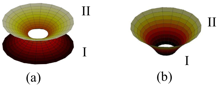
Figure 1: The bubble diagram. In figure (a), there is a domain wall on each side of the throat. In figure (b), the two domain walls of the bubble are on the same side of the throat.

3 Dynamics of the domain wall

In order to study the dynamics of the domain wall, we introduce Gaussian normal coordinates in which the metric of the spacetime is [1, 7]

$$ds^{2}=-d\tau^{2}+R(\tau,\eta)^{2}(d\theta^{2}+sin^{2}\theta d\phi^{2})+d\eta^{2}.$$ (6)

Here, $\tau$ is the proper time coordinate and $\eta$ is the proper distance away from the domain wall. The differences between various spherically symmetric metrics are described by the function $R(\tau,\eta)$, $R(\tau,\eta=0)=r_{1}$. We define $\eta$ as positive outside the domain wall and negative inside the domain wall.

Starting from the Einstein equations, one can derive the dynamical equation of the domain wall in Gaussian normal coordinates as [7]

$$\lim_{\varepsilon\rightarrow 0}[K_{ab}(\eta=+\epsilon)-K_{ab}(\eta=-\epsilon)]=-8\pi(\mathfrak{S}_{ab}-\frac{1}{2}h_{ab}\mathfrak{S}).$$ (7)

Here, $K_{ab}$ is the extrinsic curvature, $h_{ab}$ is the induced metric on the domain wall and $\mathfrak{S}_{ab}$ is the energy momentum tensor of the domain wall. $\mathfrak{S}$ represents the trace of $\mathfrak{S}_{ab}$, that is, $\mathfrak{S}=h^{ab}\mathfrak{S}_{ab}$. Equation (7) is also called the junction condition. It shows that the change in extrinsic curvature is not continuous at the location of the domain wall. Under the thin wall approximation, one can show that the relationship between $\mathfrak{S}_{ab}$ and $h_{ab}$ is [7]

$$\mathfrak{S}_{ab}=-\sigma h_{ab}.$$ (8)

Here, $\sigma$ is the surface tension of the domain wall, which is not changed with time.

For clarity, we will refer to the two domain walls as I and II. The dynamics of both domain walls are equivalent. Thus, we only need to focus on the dynamics of one of them, such as the domain wall I. For the bubble as presented in figure 1(a), inside the domain wall I is the dS spacetime and outside the domain wall I is the Schwarzschild spacetime. Thus, the 4-velocity (time-like vector) of the domain wall can be expressed as $U_{s}^{\mu}=(\dot{t}_{s},\dot{r}_{1},0,0)$ or $U_{D}^{\mu}=(\dot{t}_{D},\dot{r}_{1},0,0)$. Here, $\dot{t}_{s}=dt_{s}/d\tau$, $\dot{t}_{D}=dt_{D}/d\tau$ and $\dot{r}_{1}=dr_{1}/d\tau$. The related unit normal vectors (space-like) are $\xi_{s,\mu}=(-\dot{r}_{1},\dot{t}_{s},0,0)$ and $\xi_{D,\mu}=(\dot{r}_{1},-\dot{t}_{D},0,0)$, respectively. One can easily prove that $U_{s}^{\mu}\xi_{s,\mu}=0$ and $U_{D}^{\nu}\xi_{D,\nu}=0$ ($\mu,\nu=0,1,2,3$). Noted that $\dot{r}_{1}$ is the radial velocity of the domain wall.

The normalization condition for $U_{s}^{\mu}$ is $g_{s,\mu\nu}U_{s}^{\mu}U_{s}^{\nu}=-1$. We use $g_{s,\mu\nu}$ to represent the metric of the Schwarzschild spacetime, $g_{s,00}=-A_{s}$ and $g_{s,11}=A_{s}^{-1}$. Combining this normalization condition with equations (1) and (2), one can obtain [19]

$$A_{s}\dot{t}^{2}_{s}-A_{s}^{-1}\dot{r}_{1}^{2}=1.$$ (9)

Equation (9) can also be derived from the normalization condition $g_{s,\mu\nu}\xi_{s}^{\mu}\xi_{s}^{\nu}=1$. Similarly, the normalization condition for $U_{D}^{\mu}$ is $g_{D,\mu\nu}U_{D}^{\mu}U_{D}^{\nu}=-1$ where $g_{D,\mu\nu}$ represents the metric of the dS spacetime, $g_{D,00}=-A_{D}$ and $g_{D,11}=A_{D}^{-1}$. Combining equations (3), (4) and the normalization condition for $U_{D}^{\mu}$, one can obtain

$$A_{D}\dot{t}^{2}_{D}-A_{D}^{-1}\dot{r}_{1}^{2}=1.$$ (10)

Equation (10) can also be derived from the normalization condition $g_{D,\mu\nu}\xi_{D}^{\mu}\xi_{D}^{\nu}=1$.

Noted that $\lim_{\varepsilon\rightarrow 0}K_{ab}(\eta=-\epsilon)=\nabla_{a}\xi_{D,b}$ and $\lim_{\varepsilon\rightarrow 0}K_{ab}(\eta=+\epsilon)=\nabla_{a}\xi_{s,b}$. Combining the definition of the extrinsic curvature with equations (2), (3) and (4), one can obtain [19]

$$\lim_{\varepsilon\rightarrow 0}K_{11}(\eta=+\epsilon)=A_{s}r_{1}\dot{t}_{s}$$ (11)

and

$$\lim_{\varepsilon\rightarrow 0}K_{11}(\eta=-\epsilon)=-A_{D}r_{1}\dot{t}_{D}.$$ (12)

Bringing equation (5) into the right hand side of equation (7), we have $-8\pi(\mathfrak{S}_{11}-\frac{1}{2}h_{11}\mathfrak{S})=-4\pi\sigma r_{1}^{2}$. Combining this formula with equations (7), (11) and (12), the dynamical equation of the domain wall becomes [1, 7]

$$\beta_{D1}-\beta_{s}=\kappa r_{1}.$$ (13)

where, $\kappa=4\pi\sigma$, $\beta_{D1}$ and $\beta_{s}$ are defined as $\beta_{D1}\equiv-A_{D}\dot{t}_{D}$ and $\beta_{s}\equiv A_{s}\dot{t}_{s}$, respectively.

Combining equation (9), (10) and (13), one can show that the dynamical equation of the domain wall can also be written as [1]

$$\dot{r}_{1}^{2}+V_{1}(r_{1},M)=-1,$$ (14)

where

$$V_{1}(r_{1},M)=-(2M)^{\frac{2}{3}}(\chi^{2}+\kappa^{2})^{\frac{1}{3}}\big{\{}\frac{1}{\alpha r_{1}}+\frac{(1-\alpha^{3}r_{1}^{3})^{2}}{\gamma^{2}\alpha^{4}r_{1}^{4}}\big{\}}.$$ (15)

The parameters $\gamma^{2}$ and $\alpha$ are defined as $\gamma^{2}\equiv 4\kappa^{2}(\chi^{2}+\kappa^{2})^{-1}$ and $\alpha\equiv((\kappa^{2}+\chi^{2})/2M)^{1/3}$, respectively. In equation (14), $V_{1}(r_{1},M)$ is the effective potential of the domain wall. The variation of $V_{1}$ over $r_{1}$ is shown in figure 2. One can show that when [7]

$$r_{1}=\alpha^{-1}2^{-1/3}\big{\{}[8+(1-\gamma^{2}/2)^{2}]^{1/2}-(1-\gamma^{2}/2)\big{\}}^{1/3}\equiv r_{m},$$ (16)

$dV_{1}/dr_{1}=0$. Thus, $V_{1}(r_{m},M)$ is the maximum value of the potential $V_{1}(r_{1},M)$.

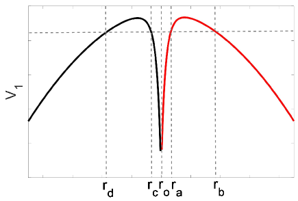
Figure 2: The diagram of the effective potential $V_{1}$. The curve of different colors represent the potentials of different domain walls. The regions $r_{o}<r_{1}<r_{a}$, $r_{o}<r_{1}<r_{c}$, $r_{1}>r_{b}$ and $r_{1}>r_{d}$ are classically allowed regions. The regions $r_{a}<r_{1}<r_{b}$ and $r_{c}<r_{1}<r_{d}$ are classically forbidden regions.

The critical mass $M_{cr}$ is defined as $V_{1}(r_{m},M_{cr})=-1$. Substituting equation (15) and (16) into the definition of $M_{cr}$, one can show that [7]

$$M_{cr}=\frac{4}{3}\pi\chi^{-3}\Lambda\cdot\frac{\gamma^{2}\alpha^{6}r_{m}^{6}(1-\gamma^{2}/4)^{1/2}}{3\sqrt{3}(\alpha^{6}r_{m}^{6}-1)^{3/2}}.$$ (17)

When $M>M_{cr}$, there is no classically forbidden region. When $M<M_{cr}$, there are two points which satisfy $\dot{r}_{1}=0$ on one side of the throat. We denote these two points as $r_{a}$ and $r_{b}$. Without loss of generality, we set $r_{a}<r_{b}$. In this study, we always assume that $r_{o}<r_{a}$. The points $r_{a}$ and $r_{b}$ are critical points that separate the classically allowed region from the classically forbidden region. The regions $r_{o}<r_{1}<r_{a}$ and $r_{1}>r_{b}$ are classically allowed regions. The region $r_{a}<r_{1}<r_{b}$ is the classically forbidden region. On the other side of the throat, another domain wall is also under the same potential. There are also two points satisfy $\dot{r}_{1}=0$. We denote these two points as $r_{c}$ and $r_{d}$ ($r_{c}<r_{d}$).

Combining equations (9), (10) and (13), one can show that the parameters $\beta_{s}$ and $\beta_{D1}$ can be expressed as [7]

$$\beta_{s}=(2M)^{\frac{1}{3}}(\chi^{2}+\kappa^{2})^{\frac{2}{3}}\cdot\frac{1-\alpha^{3}r_{1}^{3}}{2\kappa\alpha^{2}r_{1}^{2}},$$ (18)

and

$$\beta_{D1}=(2M)^{\frac{1}{3}}(\chi^{2}+\kappa^{2})^{\frac{2}{3}}\cdot\frac{1-(1-\gamma^{2}/2)\alpha^{3}r_{1}^{3}}{2\kappa\gamma^{2}r_{1}^{2}},$$ (19)

respectively. Equation (18) shows that when $r_{1}=\alpha^{-1}\equiv r_{s}$, $\beta_{s}=0$. If $\gamma^{2}\geq 2$, $\beta_{D1}$ is always positive. If $\gamma^{2}<2$, $\beta_{D1}$ can be positive or negative. In this study, we always constrain that $0<\gamma^{2}<2$. According to equation (19), one can easily show that when $r_{1}=\alpha^{-1}(1-\gamma^{2}/2)^{-1/3}\equiv r_{D}$, $\beta_{D1}=0$.

Based on the definitions of $r_{s}$ and $r_{D}$, it is useful to introduce the parameters $M_{s}$ and $M_{D}$ via the definitions $V_{1}(r_{s},M_{s})=-1$ and $V_{1}(r_{D},M_{D})=-1$, respectively. Then one can show that [7]

$$M_{s}=\frac{4}{3}\pi\chi^{-3}\Lambda(1-\gamma^{2}/4)^{1/2}$$ (20)

and

$$M_{D}=\frac{4}{3}\pi\chi^{-3}\Lambda\cdot\frac{1-\gamma^{2}/2}{1-\gamma^{2}/4}.$$ (21)

In the case where $0<\gamma^{2}<2$, one can prove that $M_{D}<M_{s}<M_{cr}$.

Figures 3 and 4 depicted the changes in the potential function $V_{1}$ as influenced by certain parameters. Different colors in these two figures represent various values of the function $-\mathrm{ln}(-V_{1})$. In figure 3, the black curve is defined as $V_{1}(r_{1},M)=-1$. The part surrounded by the black curve represents the classically forbidden region, while the other part is the classically allowed region. The red curve is defined as $\partial_{r_{1}}V_{1}=0$. The abscissa of the intersection point of the black curve and the red curve is the critical mass $M_{cr}$. When $M>M_{cr}$, there is no classically forbidden region. The purple (blue) curve is defined as $r_{1}=r_{s}$ ($r_{1}=r_{D}$). Thus, $\beta_{s}<0$ ($\beta_{D1}<0$) is above the purple (blue) curve, and $\beta_{s}>0$ ($\beta_{D1}>0$) is below the purple (blue) curve. The abscissa of the intersection point of the black curve and the purple (blue) curve is $M_{s}$ ($M_{D}$). Figure 4 illustrates that the variation of $V_{1}$ with respect to surface tension $\sigma$ is not monotonic, whereas the variation over the cosmological constant is monotonic.

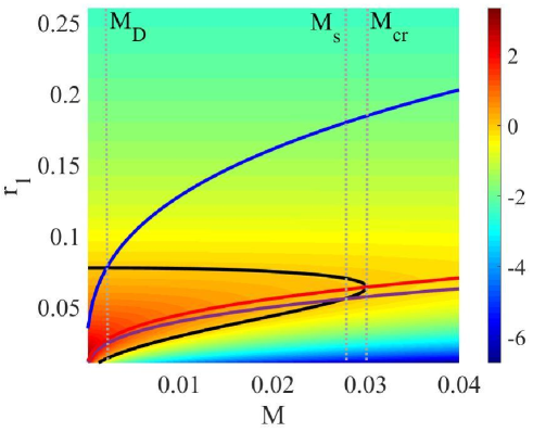
Figure 3: Diagram of the potential function $V_{1}$. The horizontal axis represents the mass parameter $M$, while the vertical axis represents the radial coordinate $r_{1}$. Various colors indicate different values of $-\mathrm{ln}(-V_{1})$. The black curve is defined as $V_{1}(r_{1},M)=-1$. The red curve is defined as $\partial_{r_{1}}V_{1}=0$. The purple curve is defined as $r_{1}=r_{s}$. The blue curve is defined as $r_{1}=r_{D}$. The parameters are taken as: $\sigma=1$, $\Lambda=20$.

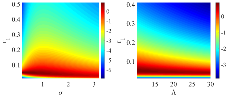
Figure 4: Diagram of the potential function $V_{1}$. Different colors in figure 4 represent various values of the function $-\mathrm{ln}(-V_{1})$. On the left panel, the horizontal axis and the vertical axis represent the surface tension $\sigma$ and the radial coordinate $r_{1}$, respectively. The parameters are taken as: $M=0.01$, $\Lambda=20$. On the right panel, the horizontal axis and the vertical axis represent the cosmological constant $\Lambda$ and the radial coordinate $r_{1}$, respectively. The parameters are taken as: $\sigma=1$, $M=0.01$.

We assume that at the initial time (the moment of completing the schwarzschild surgery), domain wall I and II are located at $r_{o1}$ and $r_{o2}$, respectively. The values of $r_{o1}$ and $r_{o2}$ are assumed to be the same, yet they are distributed in different sides of the throat. The initial state of the bubble is assumed to be $r_{o}<r_{o1}<r_{a}$ and $r_{o}<r_{o2}<r_{c}$, with $\dot{r}_{o1}>0$ and $\dot{r}_{o2}>0$. Thus, in the initial state, domain wall I is expanding and located in the classically allowed region $r_{o}<r_{1}<r_{a}$.

We consider the case where the mass parameter $M$ is smaller than the critical mass $M_{cr}$. According to equation (14), (15) and figure 2, domain wall I will expand to reach the critical point $r_{a}$. Once the radius of domain wall I reaches $r_{a}$, its radial velocity will be zero. The domain wall I will then contract until its radius reaches $r_{o}$. Equation (14) shows that the radial velocity of the domain wall is not zero at this point. Classically, the two domain walls can collide at the position of the throat. The collision of the domain walls is usually complicated and may result in the radiation of gravitational waves, the creation of black holes, and other phenomena [52, 53, 54, 55, 56, 57, 58, 59, 60]. In this study, we consider the simplest case where the collision is elastic. This means that the collision does not change the energy of the domain wall, but it does reverse its radial velocity. After the collision, the bubble will expand once again.

However, semiclassically, it is possible that domain wall I can tunnel into the classically allowed region $r_{1}>r_{b}$ through the Euclidean instanton trajectories in the classically forbidden region $r_{a}<r_{1}<r_{b}$. The instanton trajectories in the region $r_{a}<r_{1}<r_{b}$ can be described by the Euclidean version of the dynamical equation (14). That is $\dot{r}_{1,E}^{2}-V_{1}(r_{1},M)=1$, where $\dot{r}_{1,E}=dr_{1}/d\tau_{E}$ and $\tau_{E}=i\tau$. Domain wall II may tunnel into the classically allowed region $r_{1}>r_{d}$ when domain wall I reaches the position of the throat. Thus, semiclassically, it is possible that the two domain walls will not collide at the throat. Therefore, it is possible for domain wall I to pass through the throat and emerge on the other side.

When the domain wall I passes through the throat, the two domain walls will emerge on the same side of the throat, as shown in figure 1(b). The radius of domain wall I is smaller than the radius of domain wall II. On the other side of the throat and inside domain wall I, the cosmological constant is zero. Thus, in these regions, the spacetime is the Minkowski spacetime, and the metric is $ds^{2}=-dt_{M}^{2}+dx^{2}+dy^{2}+dz^{2}$. Here, $(t_{M},x,y,z)$ is the Cartesian coordinates (More strictly speaking, the spacetime in these regions is not the Minkowski spacetime if we include the influence of the matter that is introduced in the Schwarzschild surgery in order to glue two manifolds into a spacetime. However, for simplicity, we neglect the influence of this matter and approximately assume that the spacetime in these regions is Minkowski spacetime in this case. With this kind of simplification, the tunneling action corresponding to figure 1(b) can be analytically derived. Please refer to section 4.2 for detailed information. ) Outside the domain wall I and inside the domain wall II is the dS spacetime with the metric $-A_{D}dt_{D}^{2}+A_{D}^{-1}dr^{2}+r^{2}(d\theta^{2}+sin^{2}\theta d\phi^{2})$. Thus, in this case, the equation (13) can not be used to describe the dynamics of domain wall I.

Using the same methods of deriving equation (13), one can obtain the dynamical equation of domain wall I in the case of figure 1(b) as

$$\beta_{M}-\beta_{D2}=\kappa r_{1}.$$ (22)

Here,

$$\beta_{M}\equiv\dot{t}_{M}=\frac{1}{2}(\kappa+\frac{\chi}{\kappa})r_{1}$$ (23)

and

$$\beta_{D2}\equiv-A_{D}\dot{t}_{D}=\frac{1}{2}(-\kappa+\frac{\chi}{\kappa})r_{1}.$$ (24)

Noted that both $\beta_{D1}$ and $\beta_{D2}$ are formally defined as $-A_{D}\dot{t}_{D}$, yet they are different, as shown by equations (19) and (24). This is caused by the fact that in different cases, the variation of $r_{1}$ with respected to the proper time variable $\tau$ is different.

The dynamical equation (22) can also be written as

$$\dot{r}_{1}^{2}+V_{2}(r_{1})=-1,$$ (25)

where

$$V_{2}(r_{1})=-\frac{(\kappa^{2}+\chi^{2})^{2}}{4\kappa^{2}}r_{1}^{2}\equiv-(\frac{r_{1}}{r_{e}})^{2}.$$ (26)

In equation (25), $V_{2}(r_{1})$ is the effective potential of the domain wall I. In equation (26), we have defined the parameter $r_{e}\equiv 2\kappa/(\kappa^{2}+\chi^{2})$. According to equations (25) and (26), it is easily to show that $r_{1}=r_{e}$ is a critical point. In this point, $\dot{r}_{1}=0$. The region $r_{o}<r_{1}<r_{e}$ is the classically forbidden region. And the region $r_{1}>r_{e}$ is the classically allowed region. Figure 5 illustrates that the variation of $V_{2}$ with respect to surface tension $\sigma$ is not monotonic, whereas the variation over the cosmological constant $\Lambda$ or the radius $r_{1}$ is monotonic. The Euclidean version of equation (25) is $\dot{r}_{1,E}^{2}-V_{2}(r_{1})=1$. This equation described the instanton trajectories in the region $r_{o}<r_{1}<r_{e}$.

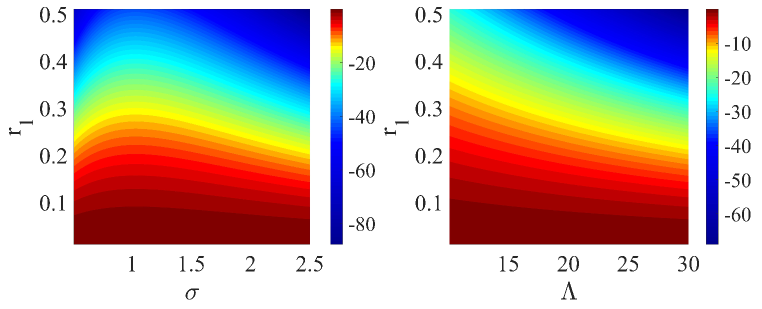
Figure 5: Diagram of the potential function $V_{2}$. Different colors in figure 5 represent various values of the function $-\mathrm{ln}(-V_{2})$. On the left panel, the horizontal axis and the vertical axis represent the surface tension $\sigma$ and the radial coordinate $r_{1}$, respectively. The parameter is taken as $\Lambda=20$. On the right panel, the horizontal axis and the vertical axis represent the cosmological constant $\Lambda$ and the radial coordinate $r_{1}$, respectively. The parameter is taken as $\sigma=1$.

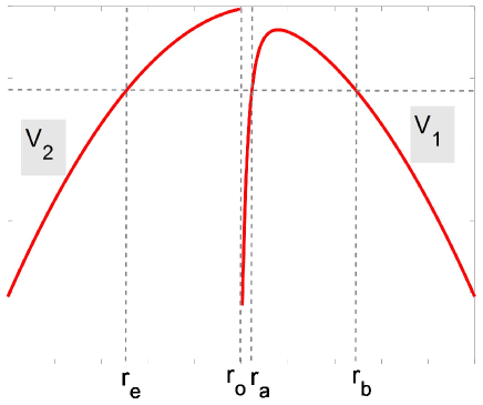
Figure 6: Diagram of the potential function $V_{1}\bigcup V_{2}$. $r_{o}$ is the radius of the throat. $r_{a}$, $r_{b}$ and $r_{e}$ are critical points of the bubble. The regions $r_{o}<r_{1}<r_{a}$, $r_{1}>r_{b}$ and $r_{1}>r_{e}$ are classically allowed regions. The regions $r_{a}<r_{1}<r_{b}$ and $r_{o}<r_{1}<r_{e}$ are classically forbidden regions.

To sum up, the bubble has two domain walls. Each of them has the effective potential $V_{1}$ on one side of the throat and another potential $V_{2}$ on the other side, as shown in figure 6. When the mass parameter $M<M_{cr}$, there are three classically allowed regions: $r_{o}<r_{1}<r_{a}$, $r_{1}>r_{b}$ and $r>r_{e}$. The classically forbidden regions are $r_{a}<r_{1}<r_{b}$ and $r_{o}<r_{1}<r_{e}$. These characteristics are different from the case where there is no wormhole. In the latter case, the bubble only has one domain wall, which only has the effective potential $V_{1}(r_{1})$. And the only classically forbidden region is $r_{a}<r_{1}<r_{b}$. We point out that in each classically forbidden region, there exists one type of instanton. Thus, we assert that the presence of the wormhole has increased the number of instantons.

4 The subtracted tunneling action

4.1 The action $S_{ab}$

In this section, we will calculate the subtracted tunneling action, which is necessary for deriving the formula for the tunneling rate. Conventionally, when a one-dimensional particle tunnels in a classically forbidden region, the subtracted tunneling action (Euclidean) is defined as [1]

$$I_{E}\equiv\int_{\tau_{i}}^{\tau_{f}}(L_{E}(x,\dot{x})-L_{E}(x,\dot{x}=0))d\tau_{E}.$$ (27)

Here, $x$ represents the dynamical variable of the particle. $\tau_{E}$ represents the Euclidean time, while $\tau_{i}$ and $\tau_{f}$ represent the moment when the particle enters and exits the classically forbidden region, respectively. $L_{E}(x,\dot{x})$ is the Euclidean Lagrangian of the particle. $L_{E}(x,\dot{x}=0)$ is the Euclidean Lagrangian at the critical point.

The subtracted tunneling action $I_{E}$ determines the characteristics of tunneling. Under the WKB approximation, the solution of the Schr$\mathrm{\ddot{o}}$dinger equation is $e^{\pm I_{E}}$. The sign ambiguity is generally presented in quantum mechanics. To describe the tunneling process, one usually chooses the exponential suppressed solution [1]. In other words, if $I_{E}$ is positive, the tunneling amplitude is $e^{-I_{E}}$, while if $I_{E}$ is negative, the tunneling amplitude is $e^{I_{E}}$. Thus, the tunneling amplitude can be expressed as $e^{-|I_{E}|}$ in any case. In this study, we follow this convention.

Both equations (14) and (25) show that the dynamics of the domain wall is similar to the one-dimensional particle. Thus, we can use the similar definition of equation (27) to calculate the subtracted tunneling action of the domain wall. Specifically, the subtracted tunneling action of the domain wall in the classically forbidden regions $r_{a}<r_{1}<r_{b}$ and $r_{o}<r_{1}<r_{e}$ are defined as

$$S_{ab}\equiv\int_{\tau_{a}}^{\tau_{b}}(L_{Eab}(r_{1},\dot{r}_{1})-L_{Eab}(r_{1},\dot{r}_{1}=0))d\tau_{E}$$ (28)

and

$$S_{oe}\equiv\int_{\tau_{o}}^{\tau_{e}}(L_{Eoe}(r_{1},\dot{r}_{1})-L_{Eoe}(r_{1},\dot{r}_{1}=0))d\tau_{E},$$ (29)

respectively. Here, $\tau_{a}$ ($\tau_{o}$) and $\tau_{b}$ ($\tau_{e}$) represent the moment when the domain wall enters and exits the classically forbidden region $r_{a}<r_{1}<r_{b}$ ($r_{o}<r_{1}<r_{e}$), respectively. $L_{Eab}(r_{1},\dot{r}_{1})$ ($L_{Eoe}(r_{1},\dot{r}_{1})$) represents the effective Euclidean Lagrangian of the domain wall in the classically forbidden region $r_{a}<r_{1}<r_{b}$ ($r_{o}<r_{1}<r_{e}$). $L_{Eab}(r_{1},\dot{r}_{1}=0)$ (or $L_{Eoe}(r_{1},\dot{r}_{1}=0)$) represents the effective Euclidean Lagrangian at the critical point.

At first, we calculate the action $S_{ab}$. According to equation (28), it is convenient to rewrite $S_{ab}$ as

$$S_{ab}=I^{tot}_{ab,E}-I^{sub}_{ab,E},$$ (30)

where $I^{tot}_{ab,E}\equiv\int_{\tau_{a}}^{\tau_{b}}L_{Eab}(r_{1},\dot{r}_{1})d\tau_{E}$ and $I^{sub}_{ab,E}\equiv\int_{\tau_{a}}^{\tau_{b}}L_{Eab}(r_{1},\dot{r}_{1}=0)d\tau_{E}$. The physical interpretation of $I^{tot}_{ab,E}$ is that it represents the Euclidean action of the bubble as it sweeps through the classically forbidden region $r_{a}<r_{1}<r_{b}$. And $I^{sub}_{ab,E}$ represents the subtracted term.

For the gravitational system, the total action is composed of the action of spacetime and the action of matter. FGG has shown that the Euclidean action $I^{tot}_{ab,E}$ of the bubble is composed of four parts [1]:

$$I^{tot}_{ab,E}=I^{wall}_{ab,matter,E}+I^{wall}_{ab,gravity,E}+I^{bulk}_{ab,matter,E}+I^{bulk}_{ab,gravity,E}.$$ (31)

Here, $I^{wall}_{ab,matter,E}$ represents the Euclidean action of the domain wall. $I^{wall}_{ab,gravity,E}$ represents the Euclidean Einstein-Hilbert action of the infinitesimal neighborhood of the domain wall. $I^{bulk}_{ab,matter,E}$ represents the Euclidean action of the false vacuum inside the domain wall. $I^{bulk}_{ab,gravity,E}$ represents the Euclidean Einstein-Hilbert action inside the domain wall. All these actions correspond to the instanton trajectory $r_{a}\rightarrow r_{b}$. Note that equation (31) is valid irrespect to whether there exist a wormhole or not.

Specifically, the four actions on the right hand side of equation (31) are defined as [1]:

$$I^{wall}_{ab,matter,E}\equiv 4\pi\sigma\int_{\tau_{a}}^{\tau_{b}}r_{1}^{2}d\tau_{E},$$ (32)

$$I^{wall}_{ab,gravity,E}\equiv-\frac{1}{16\pi}\lim_{\epsilon\rightarrow 0}\int_{-\epsilon}^{+\epsilon}d\eta\int_{\tau_{a}}^{\tau_{b}}d\tau_{E}\int d\theta d\phi r^{2}sin\theta\mathscr{R},$$ (33)

$$I^{bulk}_{ab,matter,E}\equiv-\Lambda\int_{t_{DEa}}^{t_{DEb}}dt_{DE}\int_{r_{o}}^{r_{1}}dr\int d\theta d\phi r^{2}sin\theta$$ (34)

and

$$I^{bulk}_{ab,gravity,E}\equiv-\frac{1}{16\pi}\int_{t_{DEa}}^{t_{DEb}}dt_{DE}\int_{r_{o}}^{r_{1}}dr\int d\theta d\phi r^{2}sin\theta\mathscr{R}.$$ (35)

Here, $\mathscr{R}$ is the Ricci scalar. $t_{DE}$ is the Euclidean de Sitter static coordinate time variable, i.e., $t_{DE}=it_{D}$. $t_{DEa}$ and $t_{DEb}$ represent the moment when the domain wall enters and exits the classically forbidden region $r_{a}<r_{1}<r_{b}$, respectively. Equations (32) and (34) are the Euclidean actions of the matter. Equations (33) and (35) are the Euclidean Einstein-Hilbert actions. Equations (32) and (33) are expressed in the Gaussian normal coordinates ($\tau_{E}$, $\theta$, $\phi$, $\eta$), while equations (34) and (35) are expressed in the Euclidean de Sitter static coordinates ($t_{DE}$, $r$, $\theta$, $\phi$).

The actions (32) and (33) correspond to the domain wall. They are not influenced by the Schwarzschild surgery. Thus, equations (32) and (33) are valid irrespect to whether there exists a wormhole or not. In [1], FGG showed that equation (33) can be simplified to

$$I^{wall}_{ab,gravity,E}=\int_{\tau_{a}}^{\tau_{b}}d\tau_{E}\big{\{}r_{1}(\beta_{s}-\beta_{D1})+\frac{1}{2}\ddot{r}_{1}r_{1}^{2}(\frac{1}{\beta_{D1}}-\frac{1}{\beta_{s}})-\frac{1}{4}r_{1}^{2}(\frac{1}{\beta_{D1}}\frac{dA_{D}}{dr_{1}}-\frac{1}{\beta_{s}}\frac{dA_{s}}{dr_{1}})\big{\}}.$$ (36)

Here, $\ddot{r}_{1}\equiv d^{2}r_{1}/d\tau_{E}^{2}$. After completing the integration for the variables ($r,\theta,\phi$), equation (34) becomes

$$\begin{split}I^{bulk}_{ab,matter,E}=-\frac{4}{3}\pi\Lambda\int_{t_{DEa}}^{t_{DEb}}dt_{DE}(r_{1}^{3}-r_{o}^{3})=\frac{4}{3}\pi\Lambda\int_{\tau_{a}}^{\tau_{b}}d\tau_{E}\frac{\beta_{D1}}{A_{D}}(r_{1}^{3}-r_{o}^{3}).\end{split}$$ (37)

From the first step to the second step, we used the definition $\beta_{D1}\equiv-A_{D}\dot{t}_{D}$. In equation (37), the factor $4\pi(r_{1}^{3}-r_{o}^{3})/3$ represents the comoving volume of the bubble on one side of the throat. The factor $4\pi r_{o}^{3}/3$ represents the comoving volume of the region where $r<r_{o}$, which is removed in the Schwarzschild surgery. The cosmological constant $\Lambda$ represents the energy density of the dS spacetime. Thus, the factor $4\pi\Lambda(r_{1}^{3}-r_{o}^{3})/3$ represents the energy inside the domain wall on one side of the throat. Similarly, the factor $4\pi\Lambda r_{o}^{3}/3$ represents the energy of the removed part ($r<r_{o}$) in the Schwarzschild surgery. Introducing the energy that corresponds to the comoving volume is convenient for calculating the action. We emphasize that in the absence of the wormhole, the lower limit for integrating over the variable $r_{1}$ is not $r_{1}=r_{o}$, but $r_{1}=0$.

Inside the domain wall is the dS spacetime (figure 1(a)). Based on the Einstein equations, one can show that $\mathscr{R}=-32\pi\Lambda$. Substituting this formula into equation (35) and completing the integration over the variables ($r,\theta,\phi$), then equation (35) is transformed into

$$I^{bulk}_{ab,gravity,E}=-\frac{8}{3}\pi\Lambda\int_{\tau_{a}}^{\tau_{b}}d\tau_{E}\frac{\beta_{D1}}{A_{D}}(r_{1}^{3}-r_{o}^{3}).$$ (38)

Substituting equations (32), (36), (37) and (38) into equation (31), one can obtain

$$I^{tot}_{ab,E}=\frac{4}{3}\pi\Lambda\int_{\tau_{a}}^{\tau_{b}}d\tau_{E}\frac{\beta_{D1}}{A_{D}}r_{o}^{3}+\int_{\tau_{a}}^{\tau_{b}}L_{0ab}d\tau_{E},$$ (39)

where

$$\begin{split}L_{0ab}(r_{1},\dot{r}_{1})\equiv&4\pi\sigma r_{1}^{2}-\frac{4}{3}\pi\Lambda\frac{\beta_{D1}}{A_{D}}r_{1}^{3}+r_{1}(\beta_{s}-\beta_{D1})+\frac{1}{2}r_{1}^{2}\frac{d\dot{r}_{1}}{d\tau_{E}}(\frac{1}{\beta_{D1}}-\frac{1}{\beta_{s}})\\ &-\frac{1}{4}r_{1}^{2}(\frac{1}{\beta_{D1}}\frac{dA_{D}}{dr_{1}}-\frac{1}{\beta_{s}}\frac{dA_{s}}{dr_{1}}).\end{split}$$ (40)

The first term on the right hand side of equation (39) is induced by the Schwarzschild surgery. The term $\int_{\tau_{a}}^{\tau_{b}}L_{0ab}d\tau_{E}$ represents the Euclidean action of the bubble when the wormhole vanishes. One can show that the relationship between the effective Euclidean Lagrangian $L_{Eab}(r_{1},\dot{r}_{1})$ and $L_{0ab}(r_{1},\dot{r}_{1})$ is $L_{Eab}(r_{1},\dot{r}_{1})=L_{0ab}(r_{1},\dot{r}_{1})+\frac{4}{3}\pi\Lambda r_{o}^{3}\frac{\beta_{D1}}{A_{D}}$.

For the subtracted term,

$$I^{sub}_{ab,E}=\int_{\tau_{a}}^{\tau_{b}}L_{Eab}(r_{1},\dot{r}_{1}=0)d\tau_{E}=\frac{4}{3}\pi\Lambda r_{o}^{3}\int_{\tau_{a}}^{\tau_{b}}d\tau_{E}\frac{\beta_{D1}}{A_{D}}\Big{|}_{\dot{r}_{1}=0}+\int_{\tau_{a}}^{\tau_{b}}L_{0ab}\Big{|}_{\dot{r}_{1}=0}d\tau_{E}.$$ (41)

FGG demonstrated that [1]

$$\int_{\tau_{a}}^{\tau_{b}}L_{0ab}\Big{|}_{\dot{r}_{1}=0}d\tau_{E}=\frac{1}{2}M\mathscr{T}_{\infty}.$$ (42)

Here, $\mathscr{T}_{\infty}$ represents the Euclidean Schwarzschild coordinate time measured at infinity, which corresponds to the instanton trajectory $r_{a}\rightarrow r_{b}$. When $M>M_{s}$, $\mathscr{T}_{\infty}=\int_{\tau_{a}}^{\tau_{b}}\frac{\beta_{s}}{A_{s}}d\tau_{E}$. When $M<M_{s}$, $\mathscr{T}_{\infty}=\int_{\tau_{a}}^{\tau_{b}}\frac{\beta_{s}}{A_{s}}d\tau_{E}-4\pi M$ [1]. Thus, generally,

$$\int_{\tau_{a}}^{\tau_{b}}L_{0ab}\Big{|}_{\dot{r}_{1}=0}d\tau_{E}=\frac{1}{2}M\big{\{}\int_{\tau_{a}}^{\tau_{b}}\frac{\beta_{s}}{A_{s}}d\tau_{E}-4\pi M\Theta(M_{s}-M)\big{\}}.$$ (43)

Here, $\Theta(x)$ is the Heaviside function.

Noting that at the critical point, $A_{D}=\beta_{D1}^{2}$. Substituting this equality and equation (43) into (41), the subtracted term becomes

$$I^{sub}_{ab,E}=\frac{4}{3}\pi\Lambda r_{o}^{3}\beta_{D1}^{-1}\Big{|}_{\dot{r}_{1}=0}\int_{\tau_{a}}^{\tau_{b}}d\tau_{E}+\frac{1}{2}M\big{\{}\int_{\tau_{a}}^{\tau_{b}}\frac{\beta_{s}}{A_{s}}d\tau_{E}-4\pi M\Theta(M_{s}-M)\big{\}}.$$ (44)

In addition, FGG proved that

$$\lim_{(M-M_{s})\rightarrow 0^{+}}\int_{\tau_{a}}^{\tau_{b}}\frac{\beta_{s}}{A_{s}}d\tau_{E}-\lim_{(M-M_{s})\rightarrow 0^{-}}\int_{\tau_{a}}^{\tau_{b}}\frac{\beta_{s}}{A_{s}}d\tau_{E}=4\pi M_{S}.$$ (45)

Thereby, one can easily show that the action $I^{sub}_{ab,E}$ in equation (44) is a continuous function of $M$ due to the presence of the Heaviside function related term. This is one of the reasons for choosing $\mathscr{T}_{\infty}$ as the time parameter in equation (42). Another reason for this choice is that it ensures that the classical variational principle of the bubble dynamics is well-defined. More detailed explanations can be found in [1].

Combining equation (39) and the dynamical equation (13), the action $I^{tot}_{ab,E}$ in equation (39) can be simplified as

$$I^{tot}_{ab,E}=-2\pi\sigma\int_{\tau_{a}}^{\tau_{b}}r_{1}^{2}d\tau_{E}-\frac{4}{3}\pi\Lambda\int_{\tau_{a}}^{\tau_{b}}d\tau_{E}\frac{\beta_{D1}}{A_{D}}(r_{1}^{3}-r_{o}^{3}).$$ (46)

Substituting equations (44) and (46) into equation (28), the subtracted tunneling action becomes

$$\begin{split}S_{ab}=&-2\pi\sigma\int_{\tau_{a}}^{\tau_{b}}r_{1}^{2}d\tau_{E}-\frac{4}{3}\pi\Lambda\int_{\tau_{a}}^{\tau_{b}}d\tau_{E}\frac{\beta_{D1}}{A_{D}}(r_{1}^{3}-r_{o}^{3})\\ &-\frac{4}{3}\pi\Lambda r_{o}^{3}\beta_{D1}^{-1}\Big{|}_{\dot{r}_{1}=0}\int_{\tau_{a}}^{\tau_{b}}d\tau_{E}-\frac{1}{2}M\big{\{}\int_{\tau_{a}}^{\tau_{b}}\frac{\beta_{s}}{A_{s}}d\tau_{E}-4\pi M\Theta(M_{s}-M)\big{\}}.\end{split}$$ (47)

However, this equation is only valid in the case where $M>M_{D}$.

When $M<M_{D}$, $\beta_{D1}$ starts positive and then becomes negative in the classically forbidden region $r_{a}<r_{1}<r_{b}$. Thus, in this case, $t_{DE}$ is not a monotonic function of the variable $\tau_{E}$. Therefore, the factor $\frac{4}{3}\pi\int_{\tau_{a}}^{\tau_{b}}d\tau_{E}\frac{\beta_{D1}}{A_{D}}(r_{1}^{3}-r_{o}^{3})$ does not represent the four-volume swept out by the bubble on one side of the throat when it tunnels from $r_{a}$ to $r_{b}$. It is

$$\frac{4}{3}\pi\int_{\tau_{a}}^{\tau_{b}}d\tau_{E}\frac{\beta_{D1}}{A_{D}}(r_{1}^{3}-r_{o}^{3})+\frac{4}{3}\pi(\chi^{-3}-r_{o}^{3})\pi\chi^{-1}$$ (48)

which represents the four-volume swept out by the bubble on one side of the throat. Detailed explanations about equation (48) is presented in appendix A. Therefore, for more general case, equation (47) should be modified as

$$\begin{split}S_{ab}=&-2\pi\sigma\int_{\tau_{a}}^{\tau_{b}}r_{1}^{2}d\tau_{E}-\frac{4}{3}\pi\Lambda\int_{\tau_{a}}^{\tau_{b}}d\tau_{E}\frac{\beta_{D1}}{A_{D}}(r_{1}^{3}-r_{o}^{3})-\frac{4}{3}\pi^{2}\Lambda\chi^{-1}(\chi^{-3}-r_{o}^{3})\Theta(M_{D}-M)\\ &-\frac{4}{3}\pi\Lambda r_{o}^{3}\beta_{D1}^{-1}\Big{|}_{\dot{r}_{1}=0}\int_{\tau_{a}}^{\tau_{b}}d\tau_{E}-\frac{1}{2}M\big{\{}\int_{\tau_{a}}^{\tau_{b}}\frac{\beta_{s}}{A_{s}}d\tau_{E}-4\pi M\Theta(M_{s}-M)\big{\}}.\end{split}$$ (49)

Obviously, when $r_{o}\rightarrow 0$, the action $S_{ab}$ in equation (49) goes towards the subtracted tunneling action obtained by FGG in [1]. Without the Heaviside function related terms, the action $S_{ab}$ can not be a continuous function of the mass parameter $M$ [1].

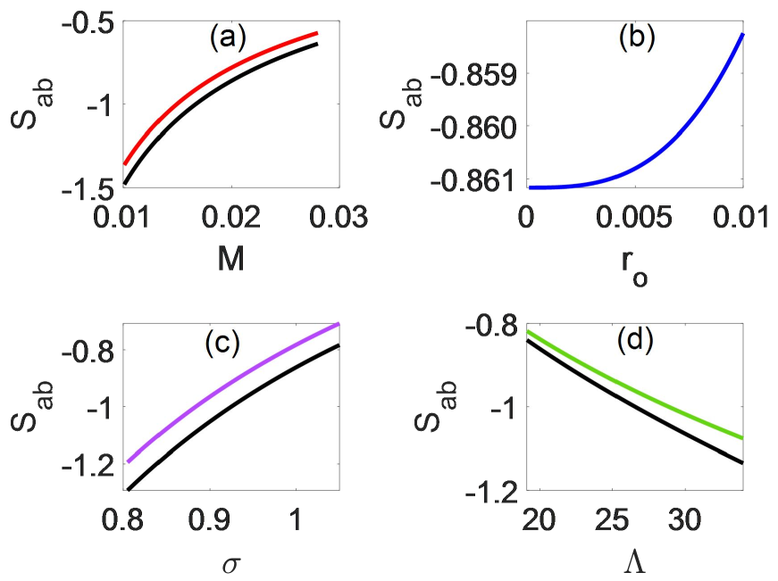
Figure 7: Variations in the subtracted tunneling action $S_{ab}$ over some parameters. In figure 7(a), the horizontal axis represents the mass parameter of the Schwarzschild spacetime. The parameters are taken as: $\sigma=1$, $r_{o}=0.03$ and $\Lambda=20$. In figure 7(b), the horizontal axis represents the radius of the throat. The parameters are taken as: $\sigma=1$, $M=0.02$ and $\Lambda=20$. In figure 7(c), the horizontal axis represents the tension of the domain wall. The parameters are taken as: $M=0.02$, $r_{o}=0.03$ and $\Lambda=20$. In figure 7(d), the horizontal axis represents the cosmological constant. The parameters are taken as: $\sigma=1$, $r_{o}=0.02$ and $M=0.02$. The black curves in figures 7(a), (c) and (d) represent the subtracted tunneling action $S_{ab}$ in the limit of $r_{o}\rightarrow 0$, while the curves of other colors represent the action $S_{ab}$ in the case where there is a wormhole.

It is difficult to analytically perform the integration over the time variable $\tau_{E}$ in equation (49). Thus, we numerically simulate certain characteristics of the action $S_{ab}$. Figure 7 shows the variations of the action $S_{ab}$ over several parameters. Figures 7(a), (b) and (c) show that the action $S_{ab}$ monotonically increases with respected to the parameters $M$, $r_{o}$ and $\sigma$. However, it monotonically decreases with the cosmological constant. In figures 7 (a), (c) and (d), the black curves represent the action $S_{ab}$ in the limit of $r_{o}\rightarrow 0$ (the wormhole disappears), while the curves of other colors represent the action $S_{ab}$ in the case of $r_{o}\neq 0$. The black curves are lower than the curves of other colors, indicating that the wormhole increased the action $S_{ab}$. The black curve in figure 7 (a) is consistent with the result obtained by FGG in [1]. Noted that $S_{ab}$ is negative within the parameters interval being considered. Thus the tunneling amplitude contributed by the instanton trajectory $r_{a}\rightarrow r_{b}$ is $e^{-|S_{ab}|}$. Therefore, figures 7(a), (b) and (c) show that the increases in the mass parameter of the black hole, the radius of the throat or the tension of the domain wall enhance the tunneling amplitude, which is associated with the instanton trajectory $r_{a}\rightarrow r_{b}$. However, the increases in the cosmological constant suppressed the tunneling amplitude $e^{-|S_{ab}|}$.

4.2 The action $S_{oe}$

For the subtracted tunneling action $S_{oe}$, which corresponds to the instanton trajectory $r_{o}\rightarrow r_{e}$, it is also composed of the Euclidean action of the bubble on one side of the throat (figure 1(b)) and the subtracted term. The Euclidean action of the bubble consists of four parts, similar to the case of equation (31). Thus, the action $S_{oe}$ can be written as

$$S_{oe}=I^{wall}_{oe,matter,E}+I^{wall}_{oe,gravity,E}+I^{bulk}_{oe,matter,E}+I^{bulk}_{oe,gravity,E}-I^{sub}_{oe,E}.$$ (50)

Here, $I^{sub}_{oe,E}$ is the subtracted term. It is defined as $I^{sub}_{oe,E}\equiv\int_{\tau_{o}}^{\tau_{e}}L_{Eoe}(r_{1},\dot{r}_{1}=0)d\tau_{E}$. The other actions (such as the surface tension related term of domain wall II) of the bubble do not influence on the tunneling of domain wall I. Thus, we have neglected them. Keeping in mind that we always focus on the dynamics of domain wall I.

The actions $I^{wall}_{oe,matter,E}$ and $I^{wall}_{oe,gravity,E}$ related to the domain wall under consideration (domain wall I). The actions $I^{bulk}_{oe,matter,E}$ and $I^{bulk}_{oe,gravity,E}$ are related to the bulk of the bubble. These four actions are defined as

$$I^{wall}_{oe,matter,E}\equiv 4\pi\sigma\int_{\tau_{o}}^{\tau_{e}}r_{1}^{2}d\tau_{E},$$ (51)

$$I^{wall}_{oe,gravity,E}\equiv-\frac{1}{16\pi}\lim_{\epsilon\rightarrow 0}\int_{-\epsilon}^{+\epsilon}d\eta\int_{\tau_{o}}^{\tau_{e}}d\tau_{E}\int d\theta d\phi r^{2}sin\theta\mathscr{R},$$ (52)

$$I^{bulk}_{oe,matter,E}\equiv\Lambda\int_{t_{DEo}}^{t_{DEe}}dt_{DE}\int_{r_{o}}^{r_{1}}dr\int d\theta d\phi r^{2}sin\theta$$ (53)

and

$$I^{bulk}_{oe,gravity,E}\equiv\frac{1}{16\pi}\int_{t_{DEo}}^{t_{DEe}}dt_{DE}\int_{r_{o}}^{r_{1}}dr\int d\theta d\phi r^{2}sin\theta\mathscr{R}.$$ (54)

Here, $t_{DEo}$ and $t_{DEe}$ represent the moment when the domain wall enters and exits the classically forbidden region $r_{o}<r_{1}<r_{e}$, respectively.

The definitions (51)-(54) are similar to the definitions (32)-(35). However, there are certain different aspects. Firstly, the actions (51)-(54) correspond to the instanton trajectory $r_{o}\rightarrow r_{e}$, while the actions (32)-(35) correspond to the instanton trajectory $r_{a}\rightarrow r_{b}$. Additionally, there is a minus sign difference between the definition (53) ((54)) and (34) ((35)). This difference is caused by the fact that in the case of definitions (34) and (35), the false vacuum region is located inside the domain wall I. However, in the case of definitions (53) and (54), the false vacuum region is located outside the domain wall I. In equation (34), the factor $-\Lambda\int_{r_{o}}^{r_{1}}dr\int d\theta d\phi r^{2}sin\theta$ implies that with the expansion of the domain wall I, the false vacuum energy increases. This is consistent with the fact that in the case of equation (34), inside the domain wall I (figure 1(a)) is the false vacuum region. With the expansion of the domain wall I, the false vacuum region increases. However, in the case of equation (53), outside the domain wall I is the false vacuum region (figure 1(b)). As the domain wall I expands, the false vacuum region decreases. In other words, the expansion of the domain wall I decreases the false vacuum energy. Thus, the factor $-\Lambda\int_{r_{o}}^{r_{1}}dr\int d\theta d\phi r^{2}sin\theta$ in the definition of (34) is replaced by $\Lambda\int_{r_{o}}^{r_{1}}dr\int d\theta d\phi r^{2}sin\theta$ in the definition of (53). Therefore, the action (53) is different from the action (34) by a minus sign. Similar explanations can be used to clarify the minus sign difference between (54) and (35).

Substituting equations (51)-(54) into equation (50), and performing the similar derivations as that in section 4.1, one can show that the subtracted tunneling action $S_{oe}$ is given by

$$S_{oe}=-\frac{4}{3}\pi\Lambda\int_{\tau_{o}}^{\tau_{e}}r_{o}^{3}\frac{\beta_{D2}}{A_{D}}d\tau_{E}+8\pi\sigma\int_{\tau_{o}}^{\tau_{e}}r_{1}^{2}d\tau_{E}-\int_{\tau_{o}}^{\tau_{e}}L_{0oe}d\tau_{E}-I^{sub}_{oe,E}$$ (55)

where

$$\begin{split}L_{0oe}(r_{1},\dot{r}_{1})\equiv&4\pi\sigma r_{1}^{2}-\frac{4}{3}\pi\Lambda\frac{\beta_{D2}}{A_{D}}r_{1}^{3}+r_{1}(\beta_{M}-\beta_{D2})\\ &+\frac{1}{2}r_{1}^{2}\frac{d\dot{r}_{1}}{d\tau_{E}}(\frac{1}{\beta_{D2}}-\frac{1}{\beta_{M}})-\frac{1}{4}r_{1}^{2}\frac{1}{\beta_{D2}}\frac{dA_{D}}{dr_{1}}.\end{split}$$ (56)

Comparing equation (29) and (55), one can show that the relationship between $L_{Eoe}(r_{1},\dot{r}_{1})$ and $L_{0oe}(r_{1},\dot{r}_{1})$ is

$$L_{Eoe}(r_{1},\dot{r}_{1})=-L_{0oe}(r_{1},\dot{r}_{1})-\frac{4}{3}\pi\Lambda r_{o}^{3}\frac{\beta_{D2}}{A_{D}}+8\pi\sigma r_{1}^{2}.$$ (57)

Noted that when $M\rightarrow 0$, the dynamical equation (14) becomes (25), $\beta_{s}\rightarrow\beta_{M}$, $\beta_{D1}\rightarrow\beta_{D2}$ and $\partial_{r_{1}}A_{s}\Big{|}_{M\rightarrow 0}=0$. Thus, $L_{0ab}(r_{1},\dot{r}_{1})\Big{|}_{M\rightarrow 0}=L_{0oe}(r_{1},\dot{r}_{1})$. Combining this equality and equation (42), one can show that

$$L_{0oe}(r_{1},\dot{r}_{1}=0)\int_{\tau_{o}}^{\tau_{e}}d\tau_{E}\propto L_{0ab}(r_{1},\dot{r}_{1}=0)\Big{|}_{M\rightarrow 0}\int_{\tau_{a}}^{\tau_{b}}d\tau_{E}=0.$$ (58)

Therefore, the subtracted term $I^{sub}_{oe,E}$ is

$$I^{sub}_{oe,E}=-\frac{4}{3}\pi\Lambda r_{o}^{3}\frac{\beta_{D2}}{A_{D}}\Big{|}_{\dot{r}_{1}=0}\int_{\tau_{o}}^{\tau_{e}}d\tau_{E}+8\pi\sigma r_{e}^{2}\int_{\tau_{o}}^{\tau_{e}}d\tau_{E}.$$ (59)

The second term on the right hand side of equation (59) used the fact that when $\dot{r}_{1}=0$, $r_{1}=r_{e}$.

Substituting equations (56) and (59) into equation (55), and using the dynamical equation (22), the action $S_{oe}$ then becomes

$$\begin{split}S_{oe}=&-2\pi\sigma\int_{\tau_{o}}^{\tau_{e}}r_{1}^{2}d\tau_{E}+\frac{4}{3}\pi\Lambda\int_{\tau_{o}}^{\tau_{e}}(r_{1}^{3}-r_{o}^{3})\frac{\beta_{D2}}{A_{D}}d\tau_{E}+\frac{4}{3}\pi\Lambda r_{o}^{3}\frac{\beta_{D2}}{A_{D}}\Big{|}_{\dot{r}_{1}=0}\int_{\tau_{o}}^{\tau_{e}}d\tau_{E}\\ &-8\pi\sigma r_{e}^{2}\int_{\tau_{o}}^{\tau_{e}}d\tau_{E}.\end{split}$$ (60)

Equation (24) shows that $\beta_{D2}$ is a monotonic function of the variable $r_{1}$. Thus, we do not need to introduce the Heaviside function in equation (60). This is different from the case of equation (49). Combining equations (60), (24), (25) and (26), the action $S_{oe}$ in equation (60) can be rewritten as

$$\begin{split}S_{oe}=-&2\pi\sigma\int_{r_{o}}^{r_{e}}r_{1}^{2}(1-\frac{r_{1}^{2}}{r_{e}^{2}})^{-1/2}dr_{1}-\frac{2}{3}\pi\Lambda r_{o}^{3}(\frac{\chi}{\kappa}-\kappa)\int_{r_{o}}^{r_{e}}r_{1}(1-\chi^{2}r_{1}^{2})^{-1}(1-\frac{r_{1}^{2}}{r_{e}^{2}})^{-1/2}dr_{1}\\ &+\frac{2}{3}\pi\Lambda(\frac{\chi}{\kappa}-\kappa)\int_{r_{o}}^{r_{e}}r_{1}^{4}(1-\chi^{2}r_{1}^{2})^{-1}(1-\frac{r_{1}^{2}}{r_{e}^{2}})^{-1/2}dr_{1}+\big{\{}\frac{2}{3}\pi\Lambda r_{o}^{3}r_{e}(\frac{\chi}{\kappa}-\kappa)\\ &\times(1-\chi^{2}r_{e}^{2})^{-1}-8\pi\sigma r_{e}^{2}\big{\}}\int_{r_{o}}^{r_{e}}(1-\frac{r_{1}^{2}}{r_{e}^{2}})^{-1/2}dr_{1}.\end{split}$$ (61)

Performing the integral over the variable $r_{1}$, the action $S_{oe}$ is transformed into

$$\begin{split}S_{oe}&=-\pi\sigma r_{e}^{3}\big{\{}r_{o}r_{e}^{-1}(1-\frac{r_{o}^{2}}{r_{e}^{2}})^{1/2}+arccos(r_{o}r_{e}^{-1})\big{\}}\\ &-\frac{2}{3}\pi\Lambda r_{o}^{3}\chi^{-1}(\frac{\chi}{\kappa}-\kappa)(r_{e}^{-2}-\chi^{2})^{-1/2}arctan\big{(}\frac{\chi(1-r_{o}^{2}r_{e}^{-2})^{1/2}}{(r_{e}^{-2}-\chi^{2})^{1/2}}\big{)}\\ &+\frac{2}{3}\pi\Lambda(\frac{\chi}{\kappa}-\kappa)\chi^{-4}\Big{\{}\frac{1}{2}r_{e}^{3}\big{\{}-(\chi^{2}-2r_{e}^{-2})arcsin(r_{e}^{-1}r_{e})-\chi^{2}r_{e}^{-1}r_{o}(1-r_{e}^{-2}r_{o}^{2})^{1/2}\\ &+(\chi^{2}-2r_{e}^{-2})arcsin(r_{e}^{-1}r_{o})\big{\}}-2r_{e}arcsin(r_{e}^{-1}r_{e})+2r_{e}arcsin(r_{e}^{-1}r_{o})\\ &-\frac{r_{e}}{2(1-\chi^{2}r_{e}^{2})^{1/2}}\big{\{}arctan\big{(}\frac{2r_{o}(r_{e}^{2}-r_{o}^{2})^{1/2}(1-\chi^{2}r_{e}^{2})^{1/2}}{\chi^{2}r_{o}^{2}r_{e}^{2}+r_{e}^{2}-2r_{o}^{2}}\big{)}-\pi\big{\}}\Big{\}}\\ &+\big{\{}\frac{2}{3}\pi\Lambda r_{o}^{3}r_{e}^{2}(\frac{\chi}{\kappa}-\kappa)(1-\chi^{2}r_{e}^{2})^{-1}-8\pi\sigma r_{e}^{3}\big{\}}\cdot\big{\{}arcsin(r_{e}r_{e}^{-1})-arcsin(r_{o}r_{e}^{-1})\big{\}}.\end{split}$$ (62)

In the appendix B, we have provided the derivation from equation (61) to (62).

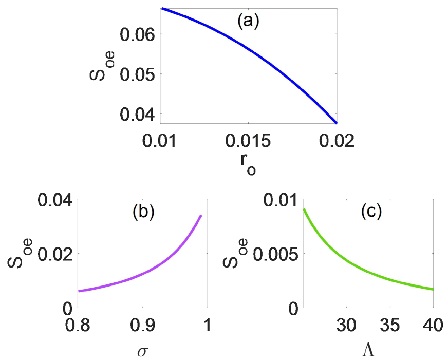
Figure 8: Variations in the subtracted tunneling action $S_{oe}$ over some parameters. In figure 8(a), the horizontal axis represents the radius of the throat. The parameters are taken as: $\sigma=1$ and $\Lambda=20$. In figure 8(b), the horizontal axis represents the tension of the domain wall. The parameters are taken as: $r_{o}=0.02$ and $\Lambda=20$. In figure 8(c), the horizontal axis represents the cosmological constant. The parameters are taken as: $\sigma=1$ and $r_{o}=0.02$ .

Figure 8 shows the variations of the action $S_{oe}$ over certain parameters. Figure 8(b) shows that the action $S_{oe}$ increases with the surface tension. Figures 8(a) and (c) show that the action $S_{oe}$ decreases with the radius of the throat and the cosmological constant. Noted that the action $S_{oe}$ is positive within the parameter intervals being considered. The tunneling amplitude contributed by the instanton trajectory $r_{o}\rightarrow r_{e}$ is $e^{-|S_{oe}|}$. Thus, figure 8 (b) shows that the increase in the surface tension suppresses the tunneling amplitude, which is associated with the instanton trajectory $r_{o}\rightarrow r_{e}$. Figures 8 (a) and (c) show that the increase in the radius of the throat or the cosmological constant enhances the tunneling amplitude $e^{-|S_{oe}|}$.

5 Tunneling rate

We have assumed that at the initial time, domain wall I is located in the classically allowed region $r_{o}<r_{1}<r_{a}$ with the radius $r_{o1}$ and the initial radial velocity $\dot{r}_{o1}>0$. Quantum mechanically, it is possible for domain wall I to pass through the classically forbidden region $r_{a}<r_{1}<r_{b}$ ($r_{o}<r_{1}<r_{e}$) and then enter the classically allowed region $r_{1}>r_{b}$ ($r_{1}>r_{e}$). In this section, we will study the tunneling rate of the process in which domain wall I tunnels from the region $r_{o}<r_{1}<r_{a}$ into other classically allowed regions.

We denote the initial time and the final time as $-T/2$ and $T/2$, respectively. We use $r_{x}$ to represent any point in the region $r_{o}<r_{1}<r_{a}$, then $r_{o}<r_{x}<r_{a}$. We use $K(r_{x},\frac{T}{2};r_{o1},-\frac{T}{2})$ to represent the amplitude of domain wall I from the state ($r_{o1}$, $-\frac{T}{2}$) evolving to the state ($r_{x}$, $\frac{T}{2}$). All trajectories in the state space which start from the state ($r_{o1}$, $-\frac{T}{2}$) and end in the state ($r_{x}$, $\frac{T}{2}$) contribute to the amplitude $K(r_{x},\frac{T}{2};r_{o1},-\frac{T}{2})$. Therefore, we need to summarize the contributions of all these trajectories.

We consider this case where the time interval ($-T/2$, $T/2$) is large enough so that for any number of collisions may have occurred during the evolution process. We can divide all these trajectories into different classes according to the number of collisions. Thus, the amplitude $K(r_{x},\frac{T}{2};r_{o1},-\frac{T}{2})$ can be expressed as

$$K(r_{x},\frac{T}{2};r_{o1},-\frac{T}{2})=\sum_{m=0}^{\infty}K^{(m)}(r_{x},\frac{T}{2};r_{o1},-\frac{T}{2}),$$ (63)

where, $K^{(m)}(r_{x},\frac{T}{2};r_{o1},-\frac{T}{2})$ represents the amplitude contributed by the classes of trajectories in which the two domain walls collide “$m$” times during the evolution process, $m=0,1,2,...$

Even in the simplest case where the two domain walls do not collide at all, there are infinite number of trajectories contribute to $K^{(0)}(r_{x},\frac{T}{2};r_{o1},-\frac{T}{2})$. We need to summarize all these contributions. Some of these trajectories are shown in figure 9. In figure 9(a), the red curve represents the classically allowed trajectory

$$r_{o1}\rightarrow r_{a}\rightarrow r_{o}\rightarrow r_{a}\rightarrow r_{o}\rightarrow\cdot\cdot\cdot\rightarrow r_{a}\rightarrow r_{x}.$$ (64)

This trajectory represents the oscillation of the domain wall I within the classically allowed region $r_{o}<r_{1}<r_{a}$. The bounce at the point $r_{o}$ is not caused by the collision of the two domain walls. It is caused by the potential $V_{2}$. And the bounce at the point $r_{a}$ is caused by the potential $V_{1}$. Equation (64) represents that the last time of the bounce has occurred at the point $r_{a}$. In fact, it is also possible that the bounce of the last time has occurred at the point $r_{o}$. However, as we have assumed that the time interval ($-T/2$, $T/2$) is large. Thus, the number of bounce is large. Consequently, the difference between the trajectory $r_{o}\rightarrow r_{x}$ and $r_{o}\rightarrow r_{a}\rightarrow r_{x}$ can be neglected when compared to the trajectory (64). In this sense, the classically allowed trajectory can always be represented by equation (64). Figures 9(b) and (e) represent that a pair of I-A-I $r_{a}\rightarrow r_{b}\rightarrow r_{a}$ and $r_{o}\rightarrow r_{e}\rightarrow r_{o}$ are inserted into the trajectory (64), respectively. Figures 9(c) and (d) represent two pairs of I-A-I $r_{a}\rightarrow r_{b}\rightarrow r_{a}$ are inserted into (64) using different methods. Figures 9(f)-(h) represent that two pairs of I-A-I $r_{o}\rightarrow r_{e}\rightarrow r_{o}$ are inserted into (64) using different methods.

The amplitude of the trajectory (64) is

$$\triangle_{o1a}e^{-S_{o1a}}\triangle_{oa}^{2(N_{1}-1)}e^{-2(N_{1}-1)S_{oa}}\triangle_{ax}e^{-S_{ax}}.$$ (65)

Here, $\triangle_{o1a}$ ($\triangle_{oa}^{2}$ or $\triangle_{ax}$) represents the fluctuation around the trajectory $r_{o1}\rightarrow r_{a}$ ($r_{o}\rightarrow r_{a}\rightarrow r_{o}$ or $r_{a}\rightarrow r_{x}$). $S_{o1a}$ ($S_{oa}$ or $S_{ax}$) represents the Euclidean action of the trajectory $r_{o1}\rightarrow r_{a}$ ($r_{o}\rightarrow r_{a}$ or $r_{a}\rightarrow r_{x}$). The factor ($N_{1}-1$) represents the number of times of the trajectory $r_{a}\rightarrow r_{o}\rightarrow r_{a}$ is repeated in trajectory (64). Equation (65) is expressed in the Euclidean proper time coordinate. Thus, the actions $S_{o1a}$, $S_{oa}$ and $S_{ax}$ all are pure imaginary numbers (i.e., the real part of these actions are zero).

Figure 9: Diagram of some of the trajectories that contribute to the amplitude of the domain wall being in the classically allowed region $r_{o}<r_{1}<r_{a}$.

Figure 9(b) represents that we inserted an I-A-I pairs ($r_{a}\rightarrow r_{b}\rightarrow r_{a}$) into the trajectory (64) when the domain wall I first arrives at the point $r_{a}$. Noted that the Euclidean action of the instanton and anti-instanton is equivalent to each other [35, 36, 61, 62]. Thus, the amplitude related to this I-A-I pairs is

$$\triangle_{ab}^{2}e^{-2|S_{ab}|}.$$ (66)

Here, $\triangle_{ab}^{2}$ represents the fluctuation around the I-A-I pairs. And $2S_{ab}$ represents the Euclidean action of a pair of I-A-I.

Figure 9(c) shows that two pairs of I-A-I are inserted into the trajectory (64) when the domain wall I first arrives at the point $r_{a}$. More generally, we can insert any pair of I-A-I into the trajectory (64) when the domain wall first arrives at the point $r_{a}$. The amplitude of all these trajectories is

$$\triangle_{o1a}e^{-S_{o1a}}\triangle_{oa}^{2(N_{1}-1)}e^{-2(N_{1}-1)S_{oa}}\triangle_{ax}e^{-S_{ax}}\sum_{m=1}^{\infty}\triangle_{ab}^{2m}e^{-2m|S_{ab}|}.$$ (67)

In equation (67), “$m$” represents the number of I-A-I pairs, which is inserted into the trajectory (64) when the domain wall I first arrive the point $r_{a}$.

In trajectory (64), everytime the domain wall I arrives at the point $r_{a}$, one can inserted any pair of I-A-I. In other words, one can insert the factor $\sum_{m=1}^{\infty}\triangle_{ab}^{2m}e^{-2m|S_{ab}|}$ at every point $r_{a}$ of trajectory (64). Similarly, one can insert the factor

$$\sum_{m=1}^{\infty}\triangle_{oe}^{2m}e^{-2m|S_{oe}|}$$ (68)

at every point $r_{o}$ of the trajectory (64). In equation (68), $\triangle_{oe}^{2}$ represents the fluctuation around a pair of I-A-I $r_{o}\rightarrow r_{e}\rightarrow r_{o}$. And $2S_{oe}$ represents the Euclidean action of a pair of I-A-I $r_{o}\rightarrow r_{e}\rightarrow r_{o}$. Noted that the number of the point $r_{a}$ in the trajectory (64) is $N_{1}$. The number of the point $r_{o}$ in the trajectory (64) is $N_{1}-1\approx N_{1}$ (we assumed $T$ is large, thus $N_{1}\gg 1$). Summarizing all of these insertion modes (also including the amplitude of the trajectory (64)), One can obtain that the amplitude $K^{(0)}(r_{x},\frac{T}{2};r_{o1},-\frac{T}{2})$ as

$$\begin{split}K^{(0)}(r_{x},\frac{T}{2};r_{o1},-\frac{T}{2})=&\triangle_{o1a}e^{-S_{o1a}}\triangle_{oa}^{2(N_{1}-1)}e^{-2(N_{1}-1)S_{oa}}\triangle_{ax}e^{-S_{ax}}\\ &\times\sum_{n=0}^{N_{1}}C_{N_{1}}^{n}(\sum_{m=1}^{\infty}\triangle_{ab}^{2m}e^{-2m|S_{ab}|})^{n}\sum_{n_{1}=0}^{N_{1}}C_{N_{1}}^{n_{1}}(\sum_{m_{1}=1}^{\infty}\triangle_{oe}^{2m_{1}}e^{-2m_{1}|S_{oe}|})^{n_{1}}.\end{split}$$ (69)

Here, $C_{N}^{n}\equiv N!/[n!(N-n)!]$. In equation (69), the term of $n=n_{1}=0$ represents the amplitude (65).

We point out that in deriving equation (69), we neglected the time spent by the I-A-I pairs $r_{a}\rightarrow r_{b}\rightarrow r_{a}$ or $r_{o}\rightarrow r_{e}\rightarrow r_{o}$. For instance, the trajectories depicted in figure 9 all correspond to the same initial time of $-T/2$ and final time of $T/2$. In other words, we have approximately treated the instanton or anti-instanton as a point on the time axis. This approximation is often employed when studying different tunneling problems using Euclidean instanton methods [36, 61, 62]. In our model, the time of the single I-A-I trajectory $r_{a}\rightarrow r_{b}\rightarrow r_{a}$ or $r_{o}\rightarrow r_{e}\rightarrow r_{o}$ can be neglected when compared to the time $T$. Thus, both the instanton and anti-instanton can be regarded as a single point on the time axis. For the multiple I-A-I trajectory $r_{a}\rightarrow r_{b}\rightarrow r_{a}\rightarrow\cdot\cdot\cdot\rightarrow r_{a}$ ($r_{o}\rightarrow r_{e}\rightarrow r_{o}\rightarrow\cdot\cdot\cdot\rightarrow r_{o}$), one may consider that the time spent by this trajectory can not be neglected when the trajectory is sufficiently long. However, this type of trajectory corresponds to a factor $e^{-2m|S_{ab}|}$ ($e^{-2m|S_{oe}|}$) with $m\gg 1$. Consequently, the influence of this type of trajectory on the amplitude $K^{(0)}(r_{x},\frac{T}{2};r_{o1},-\frac{T}{2})$ is negligible, regardless of whether we neglect the time spent by the I-A-I pairs or not. Therefore, in our model, we can always neglect the time spent by the instanton or anti-instanton.

For convenience, we define

$$Q\equiv\sum_{m=1}^{\infty}\triangle_{ab}^{2m}e^{-2m|S_{ab}|}=\frac{\triangle_{ab}^{2}e^{-2|S_{ab}|}}{1-\triangle_{ab}^{2}e^{-2|S_{ab}|}}$$ (70)

and

$$Y\equiv\sum_{m=1}^{\infty}\triangle_{oe}^{2m}e^{-2m|S_{oe}|}=\frac{\triangle_{oe}^{2}e^{-2|S_{oe}|}}{1-\triangle_{oe}^{2}e^{-2|S_{oe}|}}.$$ (71)

Substituting equations (70) and (71) into (69), the amplitude $K^{(0)}(r_{x},\frac{T}{2};r_{o1},-\frac{T}{2})$ can be simplified as

$$K^{(0)}(r_{x},\frac{T}{2};r_{o1},-\frac{T}{2})=\triangle_{o1a}e^{-S_{o1a}}\triangle_{oa}^{2(N_{1}-1)}e^{-2(N_{1}-1)S_{oa}}\triangle_{ax}e^{-S_{ax}}(1+Q)^{N_{1}}(1+Y)^{N_{1}}.$$ (72)

Comparing equation (65) and (72), one can see that if we insert the factor $(1+Q)^{N_{1}}(1+Y)^{N_{1}}$ into the amplitude (65), then we can obtain the amplitude $K^{(0)}(r_{x},\frac{T}{2};r_{o1},-\frac{T}{2})$. Each point $r_{a}$ and $r_{o}$ on the trajectory (64) corresponds to a factor $(1+Q)$ and $(1+Y)$, respectively. This indicates that at every point $r_{a}$ ($r_{o}$) on the trajectory (64), one can insert any pair of I-A-I $r_{a}\rightarrow r_{b}\rightarrow r_{a}$ ($r_{o}\rightarrow r_{e}\rightarrow r_{o}$).

Classically, the collision of the two domain walls only occurs at the position of the throat. Semiclassically, the dominant collisions also occur at the point $r_{o}$. The possibility of collision at other positions is small compared to the possibility of collision occurring at the point $r_{o}$. Thus, for simplicity, we only consider the collision occurring at the point $r_{o}$. In the later, We will show that the influence of the collision on the tunneling rate can be neglected when $T$ is large enough. This implies that our approximation (ignoring the collisions of the domain wall occurring at other positions) is reasonable.

In the case where the two domain walls collide “$m$” times, the classically allowed trajectory of domain wall I is also represented by equation (64). However, the former “$m$” bounces at the point $r_{o}$ are caused by the collision of the two domain walls. If a bounce is caused by the potential function $V_{2}$ at one time, this implies that when the domain wall I arrives at the point $r_{o}$, domain wall II has entered the classically allowed region $r_{1}>r_{d}$. Therefore, it is impossible for these two domain walls to collide again. All subsequent bounces at the point $r_{o}$ are caused by the potential $V_{2}$. Thus, the “$m$” times collisions must correspond to the former “$m$” bounces at the point $r_{o}$. After completing the “$m$” collisions, the remaining ($N_{1}-m$) bounces at the point $r_{o}$ are caused by the potential $V_{2}$. For those points $r_{o}$ where the bounce is caused by the collision of the two domain walls, one can not insert the I-A-I pair. The reason is that after each collision, the domain wall I will be bounced back into the region $r_{o}<r_{1}<r_{a}$. Consequently, there are $(N_{1}-m)$ points in the trajectory (64) where one can insert the factor $(1+Y)$. All the bounces of the domain wall I at point $r_{a}$ are caused by potential $V_{1}$. Thus, the number of points $r_{a}$ where one can insert the factor $(1+Q)$ is $N_{1}$. Therefore, the amplitude $K^{(m)}(r_{x},\frac{T}{2};r_{o1},-\frac{T}{2})$ is

$$\begin{split}K^{(m)}(r_{x},\frac{T}{2};r_{o1},-\frac{T}{2})=&\triangle_{o1a}e^{-S_{o1a}}\triangle_{oa}^{2(N_{1}-1)}e^{-2(N_{1}-1)S_{oa}}\triangle_{ax}e^{-S_{ax}}\\ &\times(1+Q)^{N_{1}}(1+Y)^{(N_{1}-m)}.\end{split}$$ (73)

When “$m=0$”, equation (73) becomes (72).

Substituting equation (73) into (63), one can obtain the amplitude $K(r_{x},\frac{T}{2};r_{o1},-\frac{T}{2})$ as

$$\begin{split}K(r_{x},\frac{T}{2};r_{o1},-\frac{T}{2})=&(1+Y)Y^{-1}\triangle_{o1a}e^{-S_{o1a}}\triangle_{oa}^{2(N_{1}-1)}e^{-2(N_{1}-1)S_{oa}}\triangle_{ax}e^{-S_{ax}}\\ &\times(1+Q)^{N_{1}}(1+Y)^{N_{1}}.\end{split}$$ (74)

The factor $(1+Y)Y^{-1}$ represents the contribution of the collisions. Comparing equations (74) and (72), one can observed that $K(r_{x},\frac{T}{2};r_{o1},-\frac{T}{2})=(1+Y)Y^{-1}K^{(0)}(r_{x},\frac{T}{2};r_{o1},-\frac{T}{2})$. Defining

$$\Omega(r_{x})\equiv(1+Y)Y^{-1}\triangle_{o1a}e^{-S_{o1a}}\triangle_{ax}e^{-S_{ax}},$$ (75)

then equation (74) can be simplified as

$$K(r_{x},\frac{T}{2};r_{o1},-\frac{T}{2})=\Omega(r_{x})\triangle_{oa}^{2(N_{1}-1)}e^{-2(N_{1}-1)S_{oa}}(1+Q)^{N_{1}}(1+Y)^{N_{1}}.$$ (76)

Equation (76) shows that the collisions, the I-A-I pairs and the classically allowed trajectory are the factors determining the amplitude $K(r_{x},\frac{T}{2};r_{o1},-\frac{T}{2})$. The instanton contributed to the amplitude $K(r_{x},\frac{T}{2};r_{o1},-\frac{T}{2})$ must be condensed to form a pair with the corresponding anti-instanton.

The probability of the domain wall I appearing at point $r_{x}$ at the moment $T/2$ is

$$P(r_{x},\frac{T}{2};r_{o1},-\frac{T}{2})=\mathscr{N}(T)K(r_{x},\frac{T}{2};r_{o1},-\frac{T}{2})K^{*}(r_{x},\frac{T}{2};r_{o1},-\frac{T}{2}).$$ (77)

Here, $\mathscr{N}(T)$ represents the normalized constant and $K^{*}(r_{x},\frac{T}{2};r_{o1},-\frac{T}{2})$ represents the complex conjugate of $K(r_{x},\frac{T}{2};r_{o1},-\frac{T}{2})$. Generally, we denote $X^{*}$ as the complex conjugate of the quantity $X$. If we denote the probability of domain wall I appearing at the classically allowed region $r_{o}<r_{1}<r_{a}$ at the moment $T/2$ as $P(r_{[o,a]},\frac{T}{2};r_{o1},-\frac{T}{2})$, then the relationship between $P(r_{[o,a]},\frac{T}{2};r_{o1},-\frac{T}{2})$ and $P(r_{x},\frac{T}{2};r_{o1},-\frac{T}{2})$ is

$$P(r_{[o,a]},\frac{T}{2};r_{o1},-\frac{T}{2})=\int_{r_{o}}^{r_{a}}dr_{x}P(r_{x},\frac{T}{2};r_{o1},-\frac{T}{2}).$$ (78)

Substituting equations (76) and (77) into equation (78), one can show that the probability $P(r_{[o,a]},\frac{T}{2};r_{o1},-\frac{T}{2})$ is given by

$$\begin{split}P(r_{[o,a]},\frac{T}{2};r_{o1},-\frac{T}{2})=&\mathscr{N}(T)\int_{r_{o}}^{r_{a}}dr_{x}\Omega(r_{x})\Omega^{*}(r_{x})\triangle_{oa}^{2(N_{1}-1)}(\triangle_{oa}^{2(N_{1}-1)})^{*}e^{-2(N_{1}-1)S_{oa}}\\ &\times e^{-2(N_{1}-1)S_{oa}^{*}}(1+Q)^{N_{1}}(1+Y)^{N_{1}}(1+Q^{*})^{N_{1}}(1+Y^{*})^{N_{1}}.\end{split}$$ (79)

Defining $\varepsilon_{0}$ as the Euclidean proper time spent by the trajectory $r_{o}\rightarrow r_{a}$, then the factor $(N_{1}-1)$ can be expressed as

$$N_{1}-1\approx\frac{T}{2\varepsilon_{0}}\approx N_{1}.$$ (80)

The approximation in equation (80) is valid in the case where $N_{1}\gg 1$ or $T\gg\varepsilon_{0}$. Substituting equation (80) into (79) and noting that the action $S_{oa}$ is a pure imaginary number (i.e., $S_{oa}^{*}=-S_{oa}$), then the probability $P(r_{[o,a]},\frac{T}{2};r_{o1},-\frac{T}{2})$ can be rewritten as

$$\begin{split}P(r_{[o,a]},\frac{T}{2};r_{o1},-\frac{T}{2})=&\mathscr{N}(T)\int_{r_{o}}^{r_{a}}dr_{x}\Omega(r_{x})\Omega^{*}(r_{x})\triangle_{oa}^{\frac{T}{\varepsilon_{0}}}(\triangle_{oa}^{\frac{T}{\varepsilon_{0}}})^{*}\\ &\times(1+Q)^{\frac{T}{2\varepsilon_{0}}}(1+Y)^{\frac{T}{2\varepsilon_{0}}}(1+Q^{*})^{\frac{T}{2\varepsilon_{0}}}(1+Y^{*})^{\frac{T}{2\varepsilon_{0}}}.\end{split}$$ (81)

The relationship between the tunneling rate $\Gamma$ and the probability $P(r_{[o,a]},\frac{T}{2};r_{o1},-\frac{T}{2})$ is [36, 62]

$$P(r_{[o,a]},\frac{T}{2};r_{o1},-\frac{T}{2})=e^{-\Gamma T}.$$ (82)

Combining equations (81) and (82), one can obtain the tunneling rate as

$$\begin{split}\Gamma=&-\frac{1}{T}\mathrm{ln}\int_{r_{o}}^{r_{a}}dr_{x}\Omega(r_{x})\Omega^{*}(r_{x})-\frac{1}{T}\mathrm{ln}\mathscr{N}(T)-\frac{1}{\varepsilon_{0}}\mathrm{ln}\triangle_{oa}\triangle_{oa}^{*}\\ &-\frac{1}{2\varepsilon_{0}}\mathrm{ln}(1+Q)(1+Y)(1+Q^{*})(1+Y^{*}).\end{split}$$ (83)

In the case where $T\gg\varepsilon_{0}$, the first term on the right hand side of equation (83) can be neglected. This implies that the contribution of the collisions can be neglected. Taking the limit of the small fluctuations, the third term on the right hand side of equation (83) can be neglected. When $\triangle_{ab}^{2}\rightarrow 1$ and $\triangle_{oe}^{2}\rightarrow 1$ (small fluctuations), according to the definitions (70) and (71), one can easily show that

$$Q\approx\frac{1}{e^{2|S_{ab}|}-1}\approx Q^{*}$$ (84)

and

$$Y\approx\frac{1}{e^{2|S_{oe}|}-1}\approx Y^{*}$$ (85)

Therefore, in the case of $T\gg\varepsilon_{0}$ and small fluctuations, the tunneling rate $\Gamma$ is given by

$$\Gamma=-\frac{1}{T}\mathrm{ln}\mathscr{N}(T)-\frac{1}{\varepsilon_{0}}\mathrm{ln}(1+Q)(1+Y).$$ (86)

It is difficult to derive the normalized constant $\mathscr{N}(T)$ from the fundamental principles of quantum mechanics. Thus, researchers often avoid discussing the normalized constant when studying the problem of bubble tunneling [10, 11]. In our model, when the wormhole disappears, the tunneling rate (86) should be equivalent to the result obtained by FGG in [1]. This feature of the tunneling rate can help us to infer certain characteristics of the normalized constant $\mathscr{N}(T)$. Specifically, when the wormhole disappears, the only classically forbidden region is $r_{a}<r_{1}<r_{b}$. There is no contribution of the I-A-I pair $r_{o}\rightarrow r_{e}\rightarrow r_{o}$. Thus, the factor $Y$ is zero. The tunneling rate (86) becomes

$$\begin{split}\Gamma&\approx-\frac{1}{T}\mathrm{ln}\mathscr{N}(T,r_{o}\rightarrow 0)-\frac{1}{\varepsilon_{0}}\mathrm{ln}(1+Q(r_{o}\rightarrow 0))\\ &\approx-\frac{1}{T}\mathrm{ln}\mathscr{N}(T,r_{o}\rightarrow 0)-\frac{1}{\varepsilon_{0}}e^{-2|S_{ab}(r_{o}\rightarrow 0)|}.\end{split}$$ (87)

Here, $\mathscr{N}(T,r_{o}\rightarrow 0)$, $Q(r_{o}\rightarrow 0)$ and $S_{ab}(r_{o}\rightarrow 0)$ represent the normalized constant $\mathscr{N}(T)$, the factor $Q$ and the action $S_{ab}$, respectively, in the limit as the wormhole disappears.

In addition, FGG showed that the tunneling amplitude of the bubble in the spacetime (3) is $e^{-|S_{ab}(r_{o}\rightarrow 0)|}$ [1]. Up to the leading order of the WKB approximation, the tunneling rate is equal to the tunneling probability [11, 63]. Thus, the tunneling rate is $e^{-2|S_{ab}(r_{o}\rightarrow 0)|}$. This result should be equivalent to the tunneling rate in equation (87). This implies that the relationship between $\mathscr{N}(T,r_{o}\rightarrow 0)$ and $Q(r_{o}\rightarrow 0)$ is

$$-\frac{1}{T}\mathrm{ln}\mathscr{N}(T,r_{o}\rightarrow 0)=\frac{1+\varepsilon_{0}}{\varepsilon_{0}}\mathrm{ln}(1+Q(r_{o}\rightarrow 0)).$$ (88)

Equation (88) shows that the function of the term $-\frac{1}{T}\mathrm{ln}\mathscr{N}(T,r_{o}\rightarrow 0)$ is to eliminate the factor $-1/\varepsilon_{0}$ in equation (87). Thus, in order to equivalent to the result obtained by FGG in the limit of the wormhole disappears, the factor $-1/\varepsilon_{0}$ in equation (86) must be eliminated by the first term on the right hand side of equation (86). Therefore, the most general form of the factor $-\frac{1}{T}\mathrm{ln}\mathscr{N}(T)$ in equation (86) is

$$-\frac{1}{T}\mathrm{ln}\mathscr{N}(T)=\frac{1+\varepsilon_{0}}{\varepsilon_{0}}\mathrm{ln}(1+Q)(1+Y)+\mathscr{X}.$$ (89)

Here, $\mathscr{X}$ represents other terms of the factor $-\frac{1}{T}\mathrm{ln}\mathscr{N}(T)$. The above arguments cannot determine the specific form of $\mathscr{X}$. In the limit of the wormhole disappears, $\mathscr{X}$ must be zero, that is, $\mathscr{X}(r_{o}\rightarrow 0)=0$.

Substituting equation (89) into (86), the tunneling rate $\Gamma$ becomes

$$\Gamma=\mathrm{ln}(1+Q)+\mathrm{ln}(1+Y)+\mathscr{X}.$$ (90)

The tunneling rate $\Gamma$ in equation (90) represents the total tunneling rate from the region $r_{o}<r_{1}<r_{a}$ into the regions $r_{1}>r_{b}$ and $r_{1}>r_{e}$. Noted that $\mathrm{ln}(1+Q)\approx e^{-2|S_{ab}|}$ ($\mathrm{ln}(1+Y)\approx e^{-2|S_{oe}|}$). This approximation represents that we neglected the contributions of the multiple I-A-I trajectories. The factor $e^{-2|S_{ab}|}$ ($e^{-2|S_{oe}|}$) represents the tunneling rate from the region $r_{o}<r_{1}<r_{a}$ into the region $r_{1}>r_{b}$ ($r_{1}>r_{e}$) contributed by the single I-A-I trajectory $r_{a}\rightarrow r_{b}\rightarrow r_{a}$ ($r_{o}\rightarrow r_{e}\rightarrow r_{o}$). This indicates that the factor $\Gamma_{1}\equiv\mathrm{ln}(1+Q)$ ($\Gamma_{2}\equiv\mathrm{ln}(1+Y)$) should be interpreted as the tunneling rate from the region $r_{o}<r_{1}<r_{a}$ into the region $r_{1}>r_{b}$ ($r_{1}>r_{e}$), which includes contributions from both single and multiple I-A-I trajectories. The domain wall I either tunnels from the region $r_{o}<r_{1}<r_{a}$ into the region $r_{1}>r_{b}$ or tunnels from the region $r_{o}<r_{1}<r_{a}$ into the region $r_{1}>r_{e}$. Thus, intuitively, $\Gamma_{1}+\Gamma_{2}$ should be equal to the total tunneling rate $\Gamma$. These arguments seems to indicate that $\mathscr{X}=0$. Therefore, the tunneling rate $\Gamma$ is

$$\Gamma=\mathrm{ln}(1+Q)(1+Y).$$ (91)

Equations (84) and (85) show that the factor $Q$ and $Y$ are positive. Thus, the tunneling rate (91) is positive. This implies that the probability of finding the domain wall I in the region $r_{o}<r_{1}<r_{a}$ decreases over time, as it may tunnel into the region $r_{1}>r_{e}$ or $r_{1}>r_{b}$. One can show that in the limit of the wormhole disappears, the tunneling rate (91) is equivalent to the result obtained by FGG.

Figure 10: Variations in the tunneling rate $\Gamma$ over some parameters. In figure 10(a), the horizontal axis represents the mass parameter of the Schwarzschild spacetime. The parameters are taken as: $\sigma=1$, $r_{o}=0.02$ and $\Lambda=20$. In figure 10(b), the horizontal axis represents the radius of the throat. The parameters are taken as: $\sigma=1$, $M=0.02$ and $\Lambda=20$. In figure 10(c), the horizontal axis represents the tension of the domain wall. The parameters are taken as: $M=0.02$, $r_{o}=0.02$ and $\Lambda=20$. In figure 10(d), the horizontal axis represents the cosmological constant. The parameters are taken as: $\sigma=1$, $r_{o}=0.02$ and $M=0.02$. The black curves in figures 10 (a), (c) and (d) represent the variations of the tunneling rate (vertical axis) over the mass parameter, tension and cosmological constant (horizontal axis), respectively, in the case where the wormhole disappears. The curves of other colors represent the variations of the tunneling rate in the case where a wormhole is present.

Figure 10 shows the variations of tunneling rate with respect to certain parameters. The black curves in figures 10 (a), (c) and (d) represent the variations of the tunneling rate over the mass parameter, tension and cosmological constant, respectively, in the case where there is no wormhole. In this case, the tunneling rate is given by $e^{-2|S_{ab}(r_{o}\rightarrow 0)|}$. The curves of other colors represent the variations of the tunneling rate when there exist a wormhole. Figure 10 shows that the presence of the wormhole enhances the tunneling rate.

Figures 10(a) and (c) show that the tunneling rate increases as the mass parameter and surface tension increases, respectively, regardless of whether there exists a wormhole or not. The increase in the mass parameter implies an increase in the effective energy of the domain wall. Thus, Figures 10(a) indicates that a higher energy of the domain wall corresponds to a faster tunneling rate. Noted that the tunneling rate depends on the absolute value of the subtracted tunneling action. Figure 7 (c) and figure 8 (b) show that both $S_{ab}$ and $S_{oe}$ increase with surface tension. However, $S_{ab}$ is negative and $S_{oe}$ is positive within the parameter intervals being considered. Thus, $|S_{ab}|$ ($|S_{oe}|$) decreases (increases) with surface tension. The conclusion obtained from figure 10 (c) is not in contrast with the conclusion obtained from figure 7 (c) and figure 8 (b). As the radius of the wormhole increases, the classically allowed region $r_{o}<r_{1}<r_{a}$ becomes smaller. The domain wall has a higher probability of arriving at the tunneling points. Thus, the tunneling rate increases with the radius of the throat. This intuitive expectation is consistent with the result shown in figure 10(b). Figures 10(d) shows that regardless of whether the wormhole exists or not, the tunneling rate decreases as the cosmological constant increases.

To derive equation (91), we made the assumption that in the initial state, the two domain walls are positioned on opposite sides of the throat and have equal radii. Thus, the dominant collisions between the domain walls take place at the throat. This assumption simplifies the derivation process. However, we have shown that the impact of the collisions on the tunneling rate can be neglected in the case of $T\gg\varepsilon_{0}$. We expect this conclusion be still valid in the case where the dominant collision occurs at other points. Setting $K^{(m)}(r_{x},\frac{T}{2};r_{o1},-\frac{T}{2})=0$ (neglecting the effect of collision), the above derivations are still valid for the case where the two domain walls have different radii in the initial state (we also need to require that domain wall II does not pass through the throat during the evolution process). Thus, one can infer that equation (91) is valid regardless of whether the radii of the two domain walls are the same or not in the initial state.

For the case where both domain walls are located at the same side of the throat at the initial time, as depicted in figure 1(b), equation (91) is not valid. Nevertheless, one can still employ the analogous approaches presented in this section to study the tunneling of the domain wall. Assuming that in the initial state, $r_{e}<r_{o1}<r_{o2}$, $r_{o2}>r_{d}$, $\dot{r}_{o1}<0$ and $\dot{r}_{o2}<0$. That is, both of these two domain walls are contracting. Before passing through the throat, the dynamics of domain wall I are described by equation (22), while the dynamics of domain wall II are described by equation (13). Up to the leading order of the WKB approximation, the amplitude of domain wall I (II) passing through the classically forbidden region $r_{o}<r_{1}<r_{e}$ ($r_{c}<r_{1}<r_{d}$) is $e^{-|S_{oe}|}$ ($e^{-|S_{ab}|}$). Subsequently, the domain wall I will cross the throat and then enter the classically allowed region $r_{o}<r_{1}<r_{a}$. For the domain wall II, after it passes through the classically forbidden region $r_{c}<r_{1}<r_{d}$ via quantum tunneling, it will enter the classically allowed region $r_{o}<r_{1}<r_{c}$. Subsequently, it may go across the throat and pass through the classically forbidden region $r_{o}<r_{1}<r_{e}$ with the tunneling amplitude $e^{-|S_{oe}|}$. Thus, the amplitude of domain wall II entering the other side of the throat is $e^{-|S_{ab}|}e^{-|S_{oe}|}$. Therefore, the tunneling probability (tunneling rate) for both of these two domain walls across the throat is

$$\Gamma=e^{-2|S_{oe}|}e^{-2|S_{ab}|}e^{-2|S_{oe}|}.$$ (92)

Equation (92) does not account for the influence of multiple instanton trajectories. One can define the different sides of the throat as different universes. Assuming that within a universe, there exists a bubble and within that bubble, there is a wormhole which is connected to another universe. These arguments suggest that the bubble can go across the throat and enter another universe through the quantum tunneling, even though it is prohibited by the classical physics.

To sum up, in this section, we have derived the tunneling rate of the bubble, which is described by equation (91). It incorporates the contributions from both single and multiple I-A-I trajectories. The normalized constant is determined according to certain arguments. Some results in figure 10 are consistent with the intuitive expectations. This indicates that the formula (91) is reasonable in some sense. Furthermore, when the wormhole vanishes, the tunneling rate (91) is equivalent to the result obtained by FGG.

6 Conclusions and discussions

In this work, we use Schwarzschild surgery to construct a wormhole. We introduce some matters to glue two manifolds into a spacetime. We have neglected the interaction between the bubble and the matters, as well as the dynamics of the throat. Usually, the topology of the wormhole is non-trivial. Thus our model may help to reveal the influence of the topology on the false vacuum bubble tunneling.

In our model, the bubble has two domain walls, we assume that at the initial time, the two domain walls are located at opposite sides of the throat. Inside the domain wall is the dS spacetime, and outside the domain wall is the Schwarzschild spacetime. The junction condition of the extrinsic curvature determines the dynamics of the domain wall. The two domain walls maybe collide at the position of the throat. For simplicity, we assume that the collision is elastic. The dynamics of the two domain walls are identical. Thus, we only focus on the dynamics of one of the domain walls. For each domain wall, there are two classically forbidden regions and three classically allowed regions if the effective energy of the domain wall is smaller than the critical mass. When the domain wall passes through the throat, its effective potential will change. And the spacetime inside the domain wall will become Minkowski spacetime.

Classically, when the effective energy is smaller than the critical mass, the domain wall cannot go across the critical point and enters other classically allowed regions. However, semiclassically, the domain wall can pass through the throat or enter other classically allowed regions through quantum tunneling. We have calculated the subtracted tunneling action in each classically forbidden region. The subtracted tunneling action is composed of five terms: the action of the matter on the domain wall, the Einstein-Hilbert action on the domain wall, the action of the matter inside the domain wall, the Einstein-Hilbert action inside the domain wall and the subtracted term.

In the case of figure 1(a), both $\beta_{s}$ and $\beta_{D1}$ are not monotonic function of the radius of the domain wall. Thus, it is necessary to introduce the Heaviside function in the subtracted tunneling action. Otherwise, the action would not be a continuous function for the mass parameter. We pointed out that in the limit when the wormhole disappears, the action is equivalent to the result obtained by FGG. We numerically simulated certain characteristics of this action and found that it monotonically increases with respect to the mass of the black hole, the radius of the throat, and the tension of the domain wall within the parameters interval being considered. However, it decreases with the cosmological constant.

For the case of figure 1(b), both $\beta_{M}$ and $\beta_{D2}$ are monotonic function of the radius of the domain wall. Thus, there is no need to introduce the Heaviside function in the subtracted tunneling action. We have derived the formula for the subtracted tunneling action analytically. We show that the action decreases with the throat radius and the cosmological constant, while it increases with the tension of the domain wall.

We have derived the formula for the tunneling rate. We summarized all the trajectories that contribute to the tunneling rate. There are two types of single I-A-I trajectories that contribute to the tunneling of the domain wall. These two types of trajectories can combine to form an infinite number of multiple I-A-I trajectories, all of which contribute to the tunneling. Our formula for the tunneling rate includes contributions from both single and multiple I-A-I trajectories. The leading order contribution comes from the single I-A-I trajectories. In the limit of the wormhole disappears, there is only one classically forbidden region. This implies that there is only one type of single I-A-I trajectory. Thus, the existence of the wormhole increases the number of instantons. This is similar to the fact that the existence of the genus usually increases the number of instantons.

Finally, we demonstrate that in the limit of a long time, the effect of the domain wall collision can be neglected. We find that as the increases of the radius of the throat, the tunneling rate also increases. We also find that an increase in the mass of the black hole and the surface tension enhances the tunneling rate. As cosmological constant increases, tunneling rate decreases. This implies that a higher energy bubble corresponds to a faster tunneling rate. We show that if there exists a wormhole within the bubble, and the wormhole is connected to another universe, then it is possible that this bubble enters another universe through quantum tunneling.

Appendix A Interpretation for equation (48)

To demonstrate that equation (48) represents the four-volume swept out by the bubble on one side of the throat when it tunnels from $r_{a}$ to $r_{b}$ in the case of $M<M_{D}$, we briefly review some results that are presented in [1]. When the wormhole disappears, the bubble only has one domain wall. Inside the domain wall there is the dS spacetime, and outside the domain wall there is the Schwarzschild spacetime. In the case of $M>M_{D}$, $\beta_{D1}$ is always positive in the classically forbidden region $r_{a}<r_{1}<r_{b}$. The factor

$$\frac{4}{3}\pi\int_{\tau_{a}}^{\tau_{b}}d\tau_{E}\frac{\beta_{D1}}{A_{D}}r_{1}^{3}$$ (93)

represents the four-volume swept out by the bubble when it tunnels from $r_{a}$ to $r_{b}$. In equation (93), $\frac{4}{3}\pi r_{1}^{3}$ represents the comoving volume of the bubble, and $\int_{\tau_{a}}^{\tau_{b}}d\tau_{E}\frac{\beta_{D1}}{A_{D}}$ represents the time spent by the bubble when it tunnels from $r_{a}$ to $r_{b}$. In the case of $M<M_{D}$, it is

$$\frac{4}{3}\pi\int_{\tau_{a}}^{\tau_{b}}d\tau_{E}\frac{\beta_{D1}}{A_{D}}r_{1}^{3}+\frac{4}{3}\pi\chi^{-3}\cdot\pi\chi^{-1}$$ (94)

represents the four-volume swept out by the bubble when it tunnels from $r_{a}$ to $r_{b}$. The second term in equation (94) is half of the four-volume of the Euclidean dS spacetime. The factor $\frac{4}{3}\pi\chi^{-3}$ represents the comoving volume of the dS spacetime. The factor $\pi\chi^{-1}$ is the time parameter. Detailed derivations about equation (94) can be found in [1].

In our model, there is a wormhole. The bubble has two domain walls. On one side of the throat, the comoving volume of the bubble is $\frac{4}{3}\pi(r_{1}^{3}-r_{o}^{3})$. Noted that the Schwarzschild surgery does not change the time parameter $\int_{\tau_{a}}^{\tau_{b}}d\tau_{E}\frac{\beta_{D1}}{A_{D}}$ and $\pi\chi^{-1}$. Thus, the first term in equation (94) should be replaced by

$$\frac{4}{3}\pi\int_{\tau_{a}}^{\tau_{b}}d\tau_{E}\frac{\beta_{D1}}{A_{D}}(r_{1}^{3}-r_{o}^{3}).$$ (95)

And the second term in equation (94) should be replaced by

$$(\frac{4}{3}\pi\chi^{-3}-\frac{4}{3}\pi r_{o}^{3})\cdot\pi\chi^{-1}.$$ (96)

Here, we have subtracted the factor $\frac{4}{3}\pi r_{o}^{3}$ as the region where $r<r_{o}$ is removed in the Schwarzschild surgery. Therefore, in the case of $M<M_{D}$, the factor

$$\frac{4}{3}\pi\int_{\tau_{a}}^{\tau_{b}}d\tau_{E}\frac{\beta_{D1}}{A_{D}}(r_{1}^{3}-r_{o}^{3})+(\frac{4}{3}\pi\chi^{-3}-\frac{4}{3}\pi r_{o}^{3})\cdot\pi\chi^{-1}$$ (97)

represents the four-volume swept out by the bubble on one side of the throat when it tunnels from $r_{a}$ to $r_{b}$.

Appendix B Derivation for equation (62)

Using the integral formula

$$\int_{a}^{1}x^{2}(1-x^{2})^{-1/2}dx=\frac{1}{2}a(1-a^{2})^{1/2}+\frac{1}{2}arccos(a),$$ (98)

one can complete the integral over the variable $r_{1}$ for the first term on the right hand side of equation (61). The result is

$$-2\pi\sigma\int_{r_{o}}^{r_{e}}r_{1}^{2}(1-\frac{r_{1}^{2}}{r_{e}^{2}})^{-1/2}dr_{1}=-\pi\sigma r_{e}^{3}\big{\{}r_{o}r_{e}^{-1}(1-\frac{r_{o}^{2}}{r_{e}^{2}})^{1/2}+arccos(r_{o}r_{e}^{-1})\big{\}}.$$ (99)

Using the integral formula

$$\int\frac{xdx}{(1-ax^{2})(1-bx^{2})^{1/2}}=-a^{-1/2}(b-a)^{-1/2}arctan(\frac{a^{1/2}(1-bx^{2})^{1/2}}{(b-a)^{1/2}}),$$ (100)

the second term on the right hand side of equation (61) becomes

$$\frac{2}{3}\pi\Lambda r_{o}^{3}(\kappa-\frac{\chi}{\kappa})\int_{r_{o}}^{r_{e}}\frac{r_{1}(1-\frac{r_{1}^{2}}{r_{e}^{2}})^{-1/2}}{1-\chi^{2}r_{1}^{2}}dr_{1}=\frac{2\pi\Lambda r_{o}^{3}(\frac{\chi}{\kappa}-\kappa)}{3\chi(r_{e}^{-2}-\chi^{2})^{1/2}}arctan\big{(}\frac{\chi(1-r_{o}^{2}r_{e}^{-2})^{1/2}}{(r_{e}^{-2}-\chi^{2})^{1/2}}\big{)}.$$ (101)

Using the following four integral formulas:

$$\begin{split}\int\frac{x^{4}dx}{(1-ax^{2})(1-bx^{2})^{1/2}}=&a^{-2}\int\frac{(1-ax^{2})dx}{(1-bx^{2})^{1/2}}-2a^{-2}\int\frac{dx}{(1-bx^{2})^{1/2}}\\ &+a^{-2}\int\frac{dx}{(1-ax^{2})(1-bx^{2})^{1/2}},\end{split}$$ (102)

$$\int\frac{(1-ax^{2})dx}{(1-bx^{2})^{1/2}}=\frac{1}{2}b^{-3/2}\big{\{}ab^{1/2}x(1-bx^{2})^{1/2}-(a-2b)arcsin(b^{1/2}x)\big{\}},$$ (103)

$$\int\frac{dx}{(1-bx^{2})^{1/2}}=b^{-1/2}arcsin(b^{1/2}x),$$ (104)

and

$$\int_{c}^{b}\frac{dx}{(1-ax^{2})(1-b^{-2}x^{2})^{1/2}}=\frac{-b}{2(1-ab^{2})^{1/2}}\big{\{}arctan\big{(}\frac{2c(b^{2}-c^{2})^{1/2}(1-ab^{2})^{1/2}}{ac^{2}b^{2}+b^{2}-2c^{2}}\big{)}-\pi\big{\}},$$ (105)

the third term on the right hand side of equation (61) becomes

$$\begin{split}&\quad\frac{2}{3}\pi\Lambda(\frac{\chi}{\kappa}-\kappa)\int_{r_{o}}^{r_{e}}r_{1}^{4}(1-\chi^{2}r_{1}^{2})^{-1}(1-\frac{r_{1}^{2}}{r_{e}^{2}})^{-1/2}dr_{1}\\ &=\frac{2}{3}\pi\Lambda(\frac{\chi}{\kappa}-\kappa)\chi^{-4}\Big{\{}\frac{1}{2}r_{e}^{3}\big{\{}-(\chi^{2}-2r_{e}^{-2})arcsin(r_{e}^{-1}r_{e})-\chi^{2}r_{e}^{-1}r_{o}(1-r_{e}^{-2}r_{o}^{2})^{1/2}\\ &\quad\quad+(\chi^{2}-2r_{e}^{-2})arcsin(r_{e}^{-1}r_{o})\big{\}}-2r_{e}arcsin(r_{e}^{-1}r_{e})+2r_{e}arcsin(r_{e}^{-1}r_{o})\\ &\quad\quad-\frac{r_{e}}{2(1-\chi^{2}r_{e}^{2})^{1/2}}\big{\{}arctan\big{(}\frac{2r_{o}(r_{e}^{2}-r_{o}^{2})^{1/2}(1-\chi^{2}r_{e}^{2})^{1/2}}{\chi^{2}r_{o}^{2}r_{e}^{2}+r_{e}^{2}-2r_{o}^{2}}\big{)}-\pi\big{\}}\Big{\}}.\end{split}$$ (106)

Using the integral formula (104), the fourth term on the right hand side of the equation (61) becomes

$$\begin{split}&\quad\big{\{}\frac{2}{3}\pi\Lambda r_{o}^{3}r_{e}(\frac{\chi}{\kappa}-\kappa)(1-\chi^{2}r_{e}^{2})^{-1}-8\pi\sigma r_{e}^{2}\big{\}}\int_{r_{o}}^{r_{e}}(1-\frac{r_{1}^{2}}{r_{e}^{2}})^{-1/2}dr_{1}\\ &=\big{\{}\frac{2}{3}\pi\Lambda r_{o}^{3}r_{e}^{2}(\frac{\chi}{\kappa}-\kappa)(1-\chi^{2}r_{e}^{2})^{-1}-8\pi\sigma r_{e}^{3}\big{\}}\cdot\big{\{}arcsin(r_{e}r_{e}^{-1})-arcsin(r_{o}r_{e}^{-1})\big{\}}.\end{split}$$ (107)

Substituting equations (99), (101), (LABEL:eq:A9) and (LABEL:eq:A10) into equation (61), one then can obtain equation (62).

References

- [1] E. Farhi, A. H. Guth and J. Guven, Is it possible to create a universe in the laboratory by quantum tunneling?, Nucl. Phys. B 339 (1990) 417.
- [2] K. Sato, M. Sasaki, H. Kodama and K. Maeda, Creation of wormholes by first order phase transition of a vacuum in the early universe, Prog. Theor. Phys. 65 (1981) 1443.
- [3] H. Kodama, M. Sasaki, K Sato and K. Maeda, Fate of wormholes created by first-order phase transition in the early universe, Prog. Theor. Phys. 66 (1981) 2052.
- [4] K. Lake, Thin spherical shells, Phys. Rev. D 19 (1979) 2847.
- [5] S. R. Coleman and F. De Luccia, Gravitational effects on and of vacuum decay, Phys. Rev. D 21 (1980) 3305.
- [6] V. A. Berezin, V. A. Kuzmin and I. I. Tkachev, Dynamics of bubbles in general relativity, Phys. Rev. D 36 (1987) 2919.
- [7] S. K. Blau, E. I. Guendelman and A. H. Guth, Dynamics of false-vacuum bubbles, Phys. Rev. D 35 (1987) 1747.
- [8] J. D. Brown and C. Teitelboim, Neutralization of the Cosmological Constant by MembraneCreation, Nucl. Phys. B 297 (1988) 787.
- [9] A. Aurilia, M. Palmer and E. Spallucci, Evolution of bubbles in a vacuum, Phys. Rev. D 40 (1989) 2511.
- [10] W. Fischler, D. Morgan, and J. Polchinski, Quantization of false-vacuum bubbles: a hamiltonian treatment of gravitational tunneling, Phys. Rev. D 42 (1990) 4042.
- [11] S. P. De Alwis, F. Muia, V. Pasquarella and F. Quevedo, Quantum transitions between Minkowski and de Sitter spacetimes, Fortschr. Phys. 68 (2020) 2000069.
- [12] W. Israel, Singular hypersurfaces and thin shells in general relativity, Nuovo Cimento 44B (1966) 1.
- [13] J. B. Hartle and S. W. Hawking, Wave function of the universe, Phys. Rev. D 28 (1983) 2960.
- [14] A. Vilenkin, Birth of inflationary universes, Phys. Rev. D 27 (1983) 2848.
- [15] A. Vilenkin, Quantum creation of the universes, Phys. Rev. D 30 (1984) 509.
- [16] A. D. Linde, Fate of the false vacuum at finite temperature: Theory and applications, Phys. Lett. B 100 (1981) 37.
- [17] A. D. Linde, Decay of the false vacuum at finite temperature, Nucl. Phys. B 216 (1983) 421.
- [18] O. Gould and J. Hirvonen, Effective field theory approach to thermal bubble nucleation, Phys. Rev. D 104 (2021) 096015.
- [19] R. Li and J. Wang, Vacuum decay and bubble nucleation in the anti-de Sitter black holes, JHEP 09 (2022) 151.
- [20] D. Saito and C.-M. Yoo, False vacuum decay in rotating BTZ spacetimes, Phys. Rev. D 104 (2021) 124037.
- [21] V. Pasquarella and F. Quevedo, Vacuum transitions in two-dimensions and their holographic interpretation, JHEP 05 (2023) 192.
- [22] J. R. Espinosaa and J.-F. Fortin, Vacuum decay actions from tunneling potentials for general spacetime dimension, JCAP 02 (2023) 023.
- [23] S. Weinberg, Cosmology, Cambridge University Press, New York (2008).
- [24] S. Dodelson, Modern cosmology, Academic press Inc., U.S. (2003).
- [25] S. H. Hawking, Wormholes in spacetime, Phys. Rev. D 37 (1988) 904.
- [26] M. Lachize-Rey and J. P. Luminet, Cosmic topology, Phys. Rep. 254 (1994) 135.
- [27] A. Anderson and B. S. DeWitt, Does the topology of space fluctuate?, Found. Phys. 16 (1986) 91.
- [28] J. Braden, M. C. Johnson, H. V. Peiris, A. Pontzen and S. Weinfurtner, New semiclassical picture of vacuum decay, Phys. Rev. Lett. 123 (2019) 031601.
- [29] K. L. Ng, B. Opanchuk, M. Thenabadu, M. Reid and P. D. Drummond, Fate of the false vacuum: finite temperature, entropy, and topological phase in quantum simulations of the early universe, PRX Quantum 2 (2021) 010350.
- [30] D. Jafferis, A. Zlokapa, J. D. Lykken, D. K. Kolchmeyer, S. I. Davis, N. Lauk, H. Neven and M. Spiropulu, Traversable wormhole dynamics on a quantum processor, Nature 612 (2022) 51.
- [31] C. Sabin, Quantum detection of wormholes, Sci. Rep. 7 (2017) 716.
- [32] K. Skenderis and B. C. van Rees, Holography and wormholes in 2+1 dimensions, Commun. Math. Phys. 301 (2011) 583–626.
- [33] S. Weigert, Topological quenching of the tunnel splitting for a particle in a double-well potential on a planar loop, Phys. Rev. A 50 (1994) 4572.
- [34] L. S. Schulman, Techniques and applications of path integration, New York: J. Wiley (1981).
- [35] S. Coleman, Fate of the false vacuum: Semiclassical theory, Phys. Rev. D 15 (1977) 2929.
- [36] C. G. Callan, Jr. and S. R. Coleman, Fate of the false vacuum. II. First quantum corrections, Phys. Rev. D 16 (1977) 1762.
- [37] J. Maldacena, The large N limit of superconformal field theories and supergravity, Adv. Theor. Math. Phys. 2 (1998) 231.
- [38] A. Kitaev, Hidden correlations in the Hawking radiation and thermal noise, Talk given at the Fundamental Physics Prize Symposium, November 10, 2014.
- [39] A. Kitaev, A simple model of quantum holography, Talks at KITP, April 7, 2015 and May 27, 2015.
- [40] S. Sachdev and J. Ye, Gapless spin fluid ground state in a random, quantum Heisenberg magnet, Phys. Rev. Lett. 70 (1993) 3339.
- [41] S. Sachdev, Holographic metals and the fractionalized Fermi liquid, Phys. Rev. Lett. 105 (2010) 151602.
- [42] J. Polchinski and V. Rosenhaus, The spectrum in the Sachdev-Ye-Kitaev model, JHEP 1604 (2016) 001.
- [43] J. Maldacena and D. Stanford, Remarks on the Sachdev-Ye-Kitaev model, Phys. Rev. D 94 (2016) 106002.
- [44] A. Kitaev and S. J. Suh, The soft mode in the Sachdev-Ye-Kitaev model and its gravity dual, JHEP 1805 (2018) 183.
- [45] P. Gao and D. L. Jafferis, A traversable wormhole teleportation protocol in the SYK model, JHEP 07 (2021) 097.
- [46] J. Maldacena and X. L. Qi, Eternal traversable wormhole, arXiv:1804.00491 [hep-th].
- [47] S. Plugge, É. Lantagne-Hurtubise and M. Franz, Revival dynamics in a traversable wormhole, Phys. Rev. Lett. 124 (2020) 221601.
- [48] T.-G. Zhou and P. Zhang, Tunneling through an eternal traversable wormhole, Phys. Rev. B 102 (2020) 224305.
- [49] M. Visser, Traversable wormholes from surgically modified Schwarzschild space-times, Nucl. Phys. B 328 (1989) 203.
- [50] S.-W. Kim, Schwarzschild—de Sitter type wormhole, Phys. Lett. A 166 (1992) 13.
- [51] J. P. S. Lemos, F. S. N. Lobo and S. Q. de Oliveira, Morris-Thorne wormholes with a cosmological constant, Phys. Rev. D 68 (2003) 064004.
- [52] Z. C. Wu, Gravitational effects in bubble collisions, Phys. Rev. D 28 (1983) 1898.
- [53] S. J. Huber and T. Konstandin, Gravitational wave production by collisions: more bubbles, JCAP 09 (2008) 022.
- [54] R. Jinno, T. Konstandin and M. Takimoto, Relativistic bubble collisions — a closer look, JCAP 09 (2019) 035.
- [55] J. Braden, J. R. Bond and L. Mersini-Houghton, Cosmic bubble and domain wall instabilities I: parametric amplification of linear fluctuations, JCAP 03 (2015) 007.
- [56] J. Braden, J. R. Bond and L. Mersini-Houghton, Cosmic bubble and domain wall instabilities II: fracturing of colliding walls, JCAP 08 (2015) 048.
- [57] J. R. Bond, J. Braden and L. Mersini-Houghton, Cosmic bubble and domain wall instabilities III: the role of oscillons in three-dimensional bubble collisions, JCAP 09 (2015) 004.
- [58] R. Gobbetti and M. Kleban, Analyzing cosmic bubble collisions, JCAP 05 (2012) 025.
- [59] M. Kleban, Cosmic bubble collisions, Class. Quantum Grav. 28 (2011) 204008.
- [60] T. John, J. Giblin, L. Hui, E. A. Lim and I.-S. Yang, How to run through walls: dynamics of bubble and soliton collisions, Phys. Rev. D 82 (2010) 045019.
- [61] U. Weiss, H. Grabert, P. Hnggi and P. Riseborough, Incoherent tunneling in a double well, Phys. Rev. B 35 (1987) 9535.
- [62] R. H. Brandenberger, Quantum field theory methods and inflationary universe models, Rev. Mod. Phys. 57 (1985) 1.
- [63] E. J. Weinberg, “Classical solutions in quantum field theory : Solitons and Instantons in High Energy Physics,” Cambridge Monographs on Mathematical Physics, September 2012.