Simulations for Meta-analysis of Magnitude Measures
Abstract
Meta-analysis aims to combine effect measures from several studies. For continuous outcomes, the most popular effect measures use simple or standardized differences in sample means. However, a number of applications focus on the absolute values of these effect measures (i.e., unsigned magnitude effects). We provide statistical methods for meta-analysis of magnitude effects based on standardized mean differences. We propose a suitable statistical model for random-effects meta-analysis of absolute standardized mean differences (ASMD), investigate a number of statistical methods for point and interval estimation, and provide practical recommendations for choosing among them.
1 Introduction
Meta-analysis aims to combine effect measures from several studies. For continuous outcomes, the most popular effect measures use simple or standardized differences in sample means. However, a number of applications focus on the corresponding magnitudes, without regard to their direction.
Meta-analyses of magnitude effects are quite common in ecology and evolutionary biology, in situations where the direction of the effect is less important. As a rationale, Garamszegi [2006] argued that “the mean of the absolute values of the effect sizes may show that weak or strong effects are at work in general without considering directional roles” or “the researcher may want to compare unsigned effect sizes between different groups of traits, such as between plumage and song traits.” Clements et al. [2022] studied the impacts of ocean acidification on fish behavior and used the absolute value “due to the inherent difficulty in assigning a functional direction to a change in behavior, as many behavioral changes can be characterized by both positive and negative functional trade-offs”. Felix et al. [2023] studied physical and chemical leaf traits that could affect herbivory but “expected the direction of the effect to be highly context-dependent (i.e., different neighbours may cause either an increase or a decrease in the same leaf trait)”. Other examples include Bailey et al. [2009] (absolute effects of plant genetic factors across levels of organization), Champagne et al. [2016] (influence of the neighboring plant on the focal plant herbivory level), and Costantini [2018] (sexual differentiation in resistance to oxidative stress across vertebrates).
Morrissey [2016] discussed the rationale for magnitude effects in evolutionary biology and proposed some statistical methods for meta-analysis of absolute mean values. We discuss his work in Section 2.1. However, the majority of the cited papers used the absolute standardized mean difference (ASMD), though some used the absolute values of Pearson correlation or log-response ratio. Interestingly, ASMD values are routinely used for testing the balance of individual covariates between the two groups of an observational study when assessing the quality of a propensity-scores-based model, with 0.1 as the standard cutoff [Rubin, 2001, Ali et al., 2019].
Typically, the systematic reviews include meta-analyses of both directional and unsigned effects. Worryingly, to meta-analyze their absolute values (magnitude effects), those reviews (Champagne et al. [2016], Costantini [2018], Clements et al. [2022], Felix et al. [2023]) use routine inverse-variance methods developed for directional effects, which have very different statistical properties. The likely explanation is the lack of statistical methods specifically for MA of magnitude effects. This article aims to fill this important gap. We develop statistical methods for meta-analysis of ASMD-based magnitude effects and study their performance by simulation.
2 Notation
We assume that each of the studies in the meta-analysis consists of two arms, Treatment and Control, with sample sizes and . The total sample size in Study is . We denote the ratio of the Control sample size to the total by . The subject-level data in each arm are assumed to be normally distributed with means and and variances and . (We appreciate, however, that real data are not exactly normal.) The sample means are , and the sample variances are , for and or .
3 Absolute mean difference
The mean difference (MD) effect measure is
with variance , estimated by
| (3.1) |
Sometimes the pooled sample variance is used instead of . Then, however, unequal variances in the Treatment and Control arms can adversely affect estimation [Kulinskaya et al., 2004].
The familiar common-effect model for MD assumes that for all , whereas the random-effects model allows the to come from a distribution with mean and variance , usually . Point estimation of often uses a weighted mean, , with in the common-effect model and in the random-effects model. Several popular methods base estimators of on , with and, initially, . We return to these methods in Section 7.2.
The underlying normal distributions in the two arms result in normality of MD: . Hence, the absolute mean difference (AMD) has a folded normal distribution (Leone et al. [1961], [Johnson et al., 1995, p.453], Tsagris et al. [2014]). For simplicity of notation, we sometimes drop the subscript .
The first two moments of the distribution are
| (3.2) |
where and are the density and the cdf of the standard normal distribution. Tsagris et al. [2014] give the moment-generating function and higher moments and the maximum-likelihood estimators of the parameters. When , is a half-normal distribution with mean and variance . A difference could be used as a centered-at-zero absolute mean effect measure, as suggested in Morrissey [2016].
From Equation (3.2), the expected depends on both the standardized mean and the variance , so AMD does not seem to be an appropriate effect measure for magnitude. Additionally, its variance is rather difficult to estimate. A naïve estimate would be . Substituting the MD and its standard deviation in the expression for in Equation (3.2) results in an biased estimate of and, therefore, of its variance. It is possible to eliminate this bias by using the second-order Taylor expansion of , but the corrected estimate appears to be rather complicated.
To summarize, dependence on the nuisance parameter , lack of asymptotic normality, and difficulty in estimating the variance of AMD preclude use of AMD in meta-analysis. Dividing in Equation (3.2) by results in a simpler expression that depends on only the standardized mean and appears to be much more convenient for further analysis, suggesting use of ASMD instead. Therefore, we abandon AMD in favor of ASMD in what follows.
4 Absolute standardized mean difference
The standardized mean difference effect measure is
The variances in the Treatment and Control arms are usually assumed to be equal. Therefore, is estimated by the square root of the pooled sample variance
| (4.1) |
The plug-in estimator , known as Cohen’s , is biased in small samples. Hedges [1983] derived the unbiased estimator
where , and
often approximated by . This estimator of , typically used in meta-analysis of SMD, is sometimes called Hedges’s .
Denote by the effective sample size in Study . The sample SMD (and therefore Hedges’s estimate ) has a scaled noncentral -distribution with noncentrality parameter (NCP) :
| (4.2) |
Therefore, the ASMD has a folded scaled noncentral -distribution with the same noncentrality parameter:
| (4.3) |
Alternatively, has a scaled noncentral distribution.
A central folded -distribution has , and a half- additionally has . The half- was introduced by Psarakis and Panaretoes [1990], who derived its moments and discussed its relations to other distributions. In particular, when , the folded converges to the folded normal distribution.
Gelman [2006] introduced the FNT distribution as a noninformative conditionally-conjugate prior for the standard deviation of the variance component in random-effects meta-analysis. However, we have not found any publications on the moments of the FNT distribution.
5 Squared standardized mean difference
The square of a FNT random variable with df has a non-central -distribution, as does the square of a noncentral random variable. As , the distribution converges to the noncentral . And when , the distribution converges to the central distribution .
The first and second moments of the noncentral distribution (the special case of the doubly-noncentral -distribution with and ) with are [Johnson et al., 1995, (30.3)]
| (5.1) |
From Equation (4.2),
Using and in Equation (5.1), the moments of are
| (5.2) |
| (5.3) |
From Equation (5.2), an unbiased estimate of the squared SMD is
| (5.4) |
The variance of is
| (5.5) |
Combining Equations (5.4) and (5.5),
Hence,
Substituting from Equation (5.4) and the above estimate of into Equation (5.5), we obtain an unbiased estimate of :
| (5.6) |
The related problem of estimating the noncentrality from a single observation from is well investigated. The UMVUE estimator is , which, for our setting, becomes but is inadmissible, as is its truncated-at-zero version. See [Johnson et al., 1995, Section 30.6] for discussion of point and interval estimation of .
Steiger [2004] provides an explicit algorithm for finding a confidence interval for the noncentrality parameter of a noncentral distribution based on an inverted test. We obtain a confidence interval for as follows:
-
•
Calculate .
-
•
If , . Otherwise, solve for in .
-
•
If , . Otherwise, solve for in .
-
•
The confidence interval for is , and taking the square root of these estimated confidence limits yields the confidence interval for .
The above equations for the confidence limits have a unique solution because is a decreasing function of . We call these confidence intervals, based on inverted or tests, - or -profile intervals.
6 Meta-analysis of squared SMD
We assume that the studies, with sample sizes in the Control and Treatment arms, respectively, resulted in magnitude effects or . We formulate common-effect and random effects models (REM) for magnitude effects in sections 6.1 and 6.2, respectively. Inference for under REM is discussed in sections 6.3 and 6.4.
6.1 Common-effect model for
We formulate the common-effect model (also known as the fixed-effect model) for the magnitude effect as
| (6.1) |
The objective is to estimate the magnitude .
From Equation (5.4), any weighted average of the is an unbiased estimate of . The simplest choice uses weights proportional to . Then
| (6.2) |
is distributed as a shifted and scaled sum of -distributed r.v.’s. Also, the simpler statistic
| (6.3) |
This distribution appears rather complicated, and we are not aware of any publications or implementations of it. When , it converges to a scaled (by ) sum of distributions, which is just a scaled noncentral distribution [Johnson et al., 1995, (29.5)]:
| (6.4) |
The statistic can be used to test for using the percentage points of the central distribution, in the case of large sample sizes, or of the central version of Equation (6.3) directly by using the parametric bootstrap. An algorithm similar to that at the end of Section 5 can be used to obtain an approximate -level -profile confidence interval for .
6.2 Random-effects model for
We formulate the random-effects model for the magnitude effect as
| (6.5) |
The model for the is the standard random-effects model, with parameters and . The objective, however, is to estimate instead of . From we obtain .
The distribution of in Equation (6.5) is conditional on . Taking into account the distribution of , has a noncentral -distribution mixed over its noncentrality parameter. By definition, the doubly-noncentral -distribution is the distribution of the ratio of two independent noncentral chi-square random variables: , where and . Corollary 2 of Jones and Marchand [2021] states that if and and independently, then .
For , we take , , , , and and write to obtain
| (6.6) |
When , Equation (6.6) is still valid and reduces to Equation (6.1); that is, the random-effects model becomes the common-effect model. Under the REM,
. Therefore, given by Equation (6.2) or any other weighted mean of the with constant weights would provide an unbiased estimate of .
6.3 Inference for from signed values of SMD
When the initial meta-analysis used the and estimated by , we can obtain a point estimate of the magnitude effect as or its truncated-at-zero version.
It is convenient to consider using a level confidence interval for , , as the basis for a level confidence interval for .
By we denote a level- CI for with level . To allow unequal division of between the two tails, we let be the part in the upper tail. , , is the estimated standard deviation of , and is the critical value at tail area from an appropriate symmetric distribution , such as normal or t.
When both confidence limits are on the same side of zero, say (i.e., when ), the naïve CI provides a CI for with level for some because also includes the values of in . This extra coverage probability is
| (6.7) |
When , the probability decreases from .025 when to 4.43e-05 when to 2.052e-09 when . The case yields the same values when . The extra coverage seems small enough not to require correction of the confidence level.
However, to obtain exactly level coverage for for an arbitrary , take, for simplicity, , substitute for in Equation (6.7), and solve for in the equation .
Similarly, when or, equivalently, when , we can choose the naïve confidence interval for . This interval provides a CI for with level . Suppose . Then also includes values of for which , which were not included in the initial level- CI for . Thie extra coverage probability is
| (6.8) |
When , the probability decreases from .025 when to 1.84e-04 when to 1.242e-08 when .
To obtain exactly -level coverage when , we can choose a value of so that and take the corrected interval as a level CI for . This is equivalent to finding such that . This equation always has a solution: when , , and when , .
Our simulations included the above correction to the naïve confidence interval for .
6.4 Conditional inference for given
Section 6.3 suggests the point estimate for the magnitude effect (conditional on ). Obtaining a confidence interval for given is more complicated because and are not independent. A simple way forward uses Equation (6.6) and the statistic
| (6.9) |
A conditional (given ) test for would compare against a percentile from the distribution, or a critical value obtained by bootstrapping the distribution of . In the same vein, to obtain a conditional (given ) -profile confidence interval for , we can substitute for in Equation (6.9) and solve for the confidence limits for at the .025 and .975 percentage points.
7 Simulation study
7.1 Simulation design
A number of other studies have used simulation to examine estimators of or of the overall effect for SMD. Our simulation design largely follows that of Bakbergenuly et al. [2020], which includes a detailed summary of previous simulation studies and gives our rationale for choosing the ranges of values for , , and that we consider realistic for a range of applications.
All simulations used the same numbers of studies () and, for each combination of parameters, the same vector of total sample sizes and the same proportion of observations in the Control arm ( for all ). Thus, the sample sizes in the Treatment and Control arms were approximately equal: and , .
We studied equal and unequal study sizes. For equal-sized studies, the sample sizes were . In choosing unequal study sizes, we followed a suggestion of Sánchez-Meca and Marín-Martínez [2000], who selected sets of study sizes having skewness 1.464, which they considered typical in behavioral and health sciences. Table 1 gives the details.
We used a total of repetitions for each combination of parameters. Thus, the simulation standard error for estimated coverage of , or at the confidence level is roughly .
The simulations were programmed in R version 4.0.2.
| Squared SMD | Equal study sizes | Unequal study sizes |
|---|---|---|
| (number of studies) | 5, 10, 20, 30, 50, 100 | 5, 10, 30 |
| or (average (individual) study size | 40, 100, 250, 500 | 60 (24,32,36,40,168), |
| — total of the two arms) | 100 (64,72,76,80,208), | |
| For and , the same set of unequal | 160 (124,132,136,140,268) | |
| study sizes was used twice or six times, respectively. | ||
| (proportion of observations in the Control arm) | 1/2 | 1/2 |
| (true value of the SMD) | 0, 0.2, 0.5, 1, 2 | 0, 0.2, 0.5, 1, 2 |
| (variance of random effects) | 0(0.1)1 | 0(0.1)1 |
We varied four parameters: the overall true SMD (), the between-studies variance (), the number of studies (), and the studies’ total sample size ( and ). Table 1 lists the values of each parameter.
We generated the true effect sizes from a normal distribution: . We generated the values of directly from the appropriately scaled noncentral -distribution, , and obtained the values of Hedges’s and for further meta-analysis of SMD and of ASMD, respectively.
7.2 Tests and estimators studied
Under the random-effects model for SMD, we used the generated values of Hedges’s to calculate the three estimators of (MP, KDB, and SSC) that Bakbergenuly et al. [2020] and Bakbergenuly et al. [2022] recommended as the best available. Briefly, Mandel and Paule [1970] (MP) estimator is based on the first moment of the large-sample chi-square distribution of Cochran’s . Kulinskaya et al. [2011] derived corrections to moments of . The KDB estimator is a moment-based estimator based on this improved approximation. A generalised statistic discussed in DerSimonian and Kacker [2007] and further studied for SMD by Bakbergenuly et al. [2020] and Bakbergenuly et al. [2022], allows the weights to be arbitrary positive constants. The SSC estimator is a moment-based estimator with effective sample size weights .
As a baseline, we recorded the bias of these three estimators and the bias of the three point estimators of that used the MP, KDB, or SSC estimate of in the weights.
Point estimators for are weighted averages of estimated SMDs . Estimators corresponding to MP and KDB ( and ) use inverse-variance-weights obtained by substitution of MP or KDB estimator of into expression for an inverse-variance-weights . The SSC point estimator of uses effective sample size weights .
Under the common-effect model for ASMD, we studied bias of , empirical levels and power of a chi-square test for based on (Equation (6.3)), and coverage of the chi-square profile confidence interval for at the 95% nominal level.
In random-effects meta-analysis of ASMD, we studied the bias of three point estimators of (, , and ) calculated as , where is given by Equation (6.2) and is given by the corresponding estimator of , and of their truncated-at-zero versions, calculated as .
We studied coverage of the 95% confidence intervals for based on the confidence intervals for the signed values, described in Section 6.3. We considered both naïve and corrected versions of these CIs . We used percentage points from the normal distribution for the MP, KDB, and SSC-based intervals and percentage points for a second SSC-based interval, denoted by SSC_t.
Interval estimators for corresponding to MP, KDB and SSC use the respective point estimator as the midpoint, and the half-width equals the estimated standard deviation of under the random-effects model times the critical value from the normal or (for SSC_t) from the distribution on degrees of freedom.
We also studied coverage of the three conditional 95% confidence intervals for , , and based on the statistic given by Equation (6.9) in combination with the estimates , , and .
Additionally, we studied empirical levels and power of the conditional tests of based on the statistics , , and and the distribution or the approximation to this distribution (Equation (6.9)). For comparison, we also studied empirical levels of the unconditional test based on for known .
8 Simulation results
8.1 Baseline estimation of and
In estimation of , the maximum average bias across all configurations was below , and the median bias was or less for all three estimators.
In estimation of , the maximum bias was higher, at 0.045 or less, but it decreased to 0.017 or less for . The median bias was less than 0.0015.
Bakbergenuly et al. [2020, 2022] give more details on the behavior of our chosen estimators.
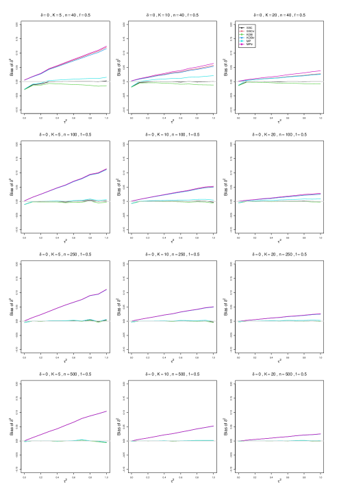
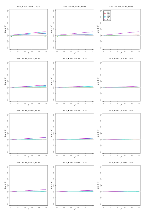
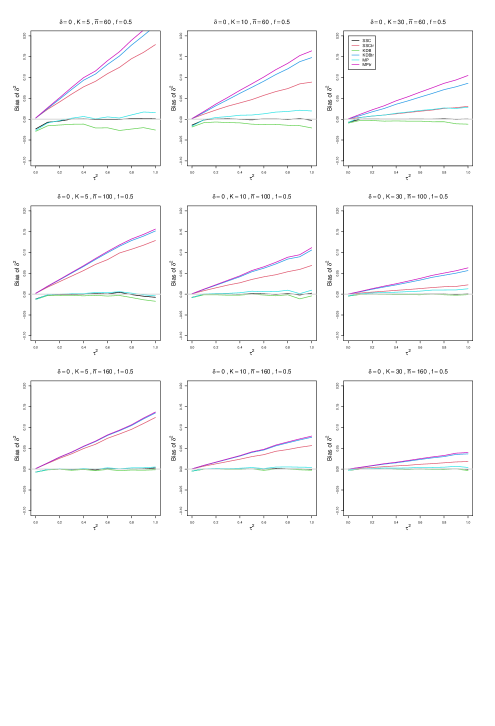
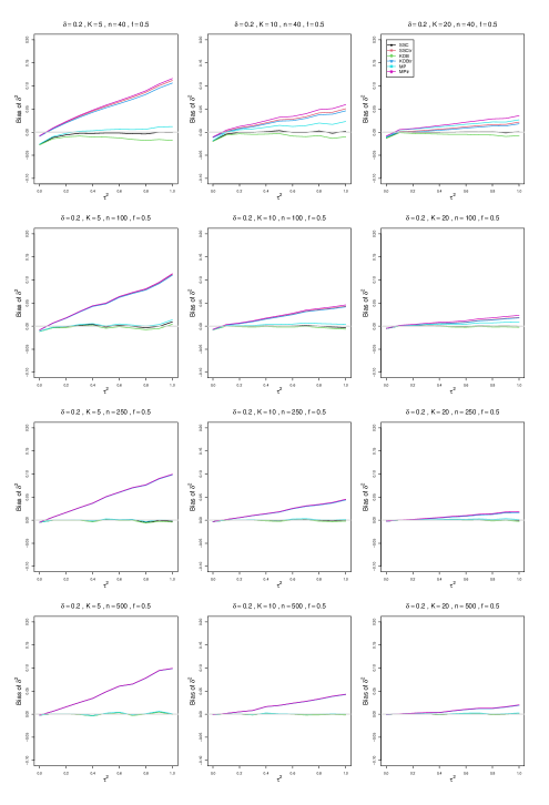
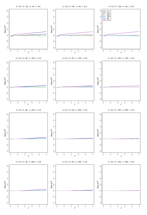
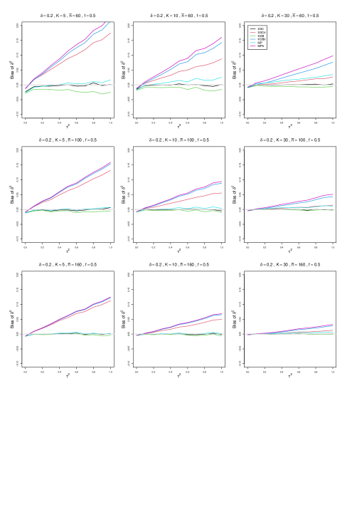
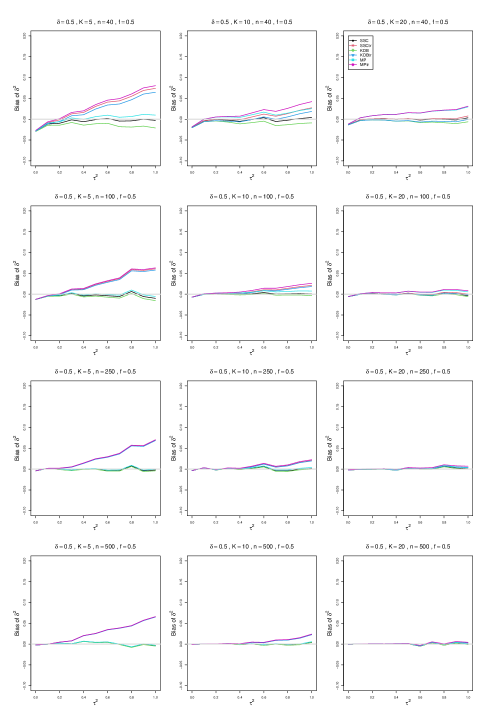
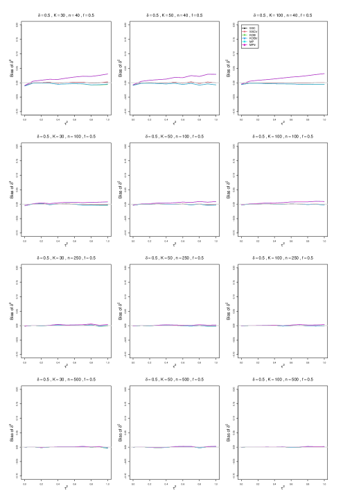
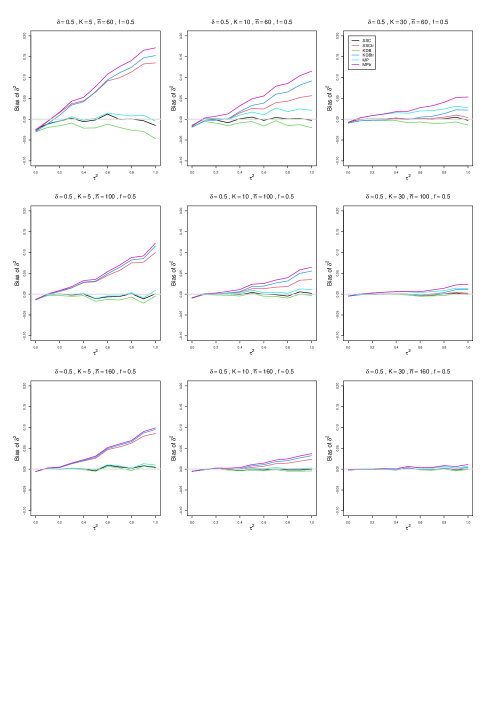
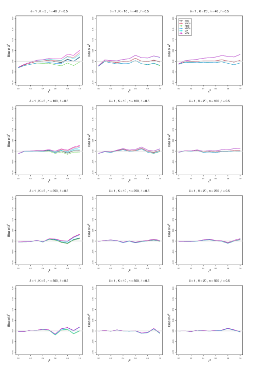
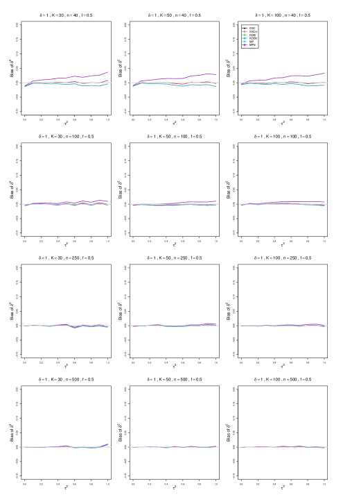
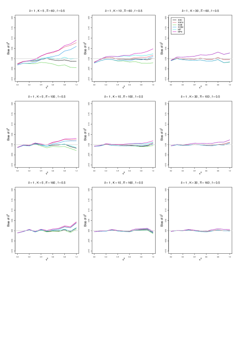
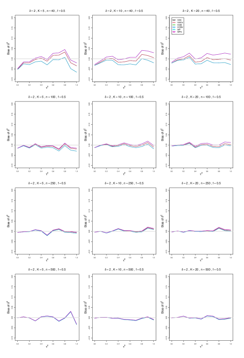
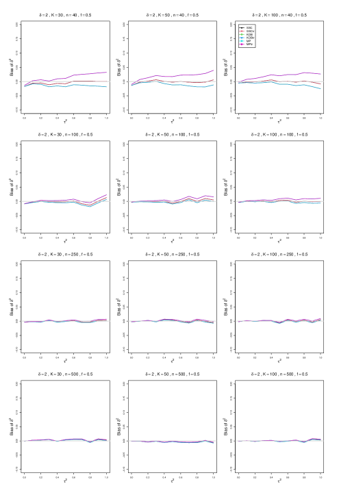
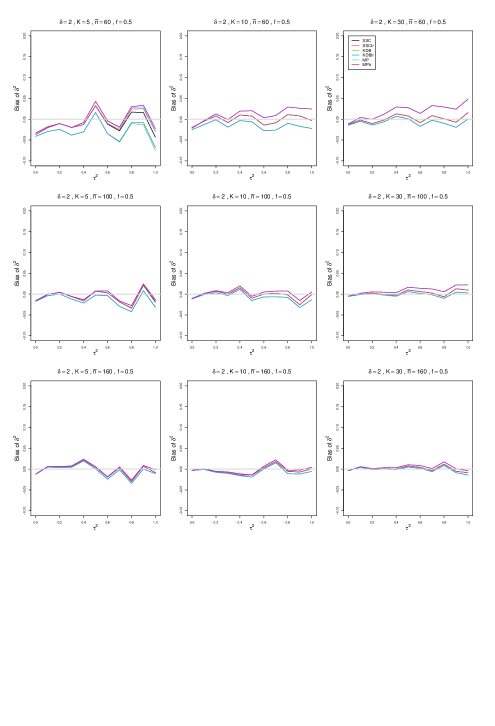
8.2 Bias of point estimators of , Appendix A
When , all three estimators had a small negative bias for , but were almost unbiased for . The truncated versions had positive bias, especially pronounced for , that increased with increasing . SSC was almost unbiased. For larger values of , bias varied more among the estimators when and . However, for larger , the bias of all estimators was very small.
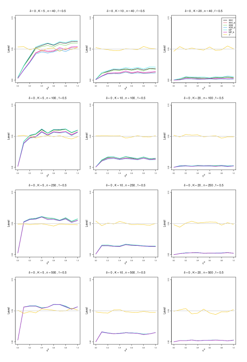
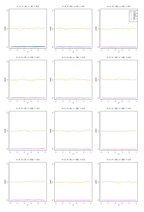
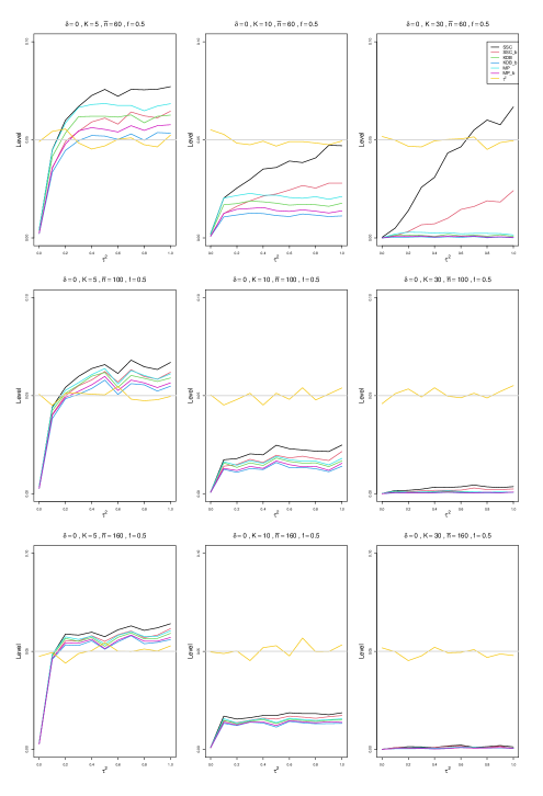
8.3 Empirical levels of the conditional tests of , Appendix B
All three conditional tests of at a 5% nominal level proved unfit for use. The levels were near zero when , but when , they increased to near nominal for and increased to about 0.06 by . The tests based on the bootstrap values behaved similarly, with somewhat lower levels. However, for , the levels increased to about 0.02 and remained there, and for they were near zero for all values. In contrast, the unconditional test, which used known , produced consistent near-nominal levels. We believe that the disappointing behavior of the conditional tests arises from high correlation between the and values. This correlation is well known for the folded normal distribution [Tsagris et al., 2014].
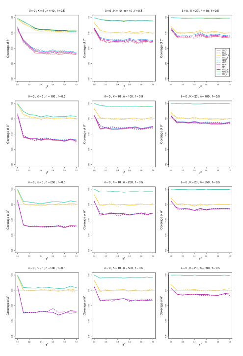
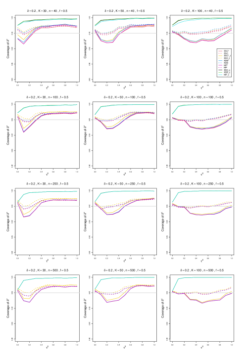
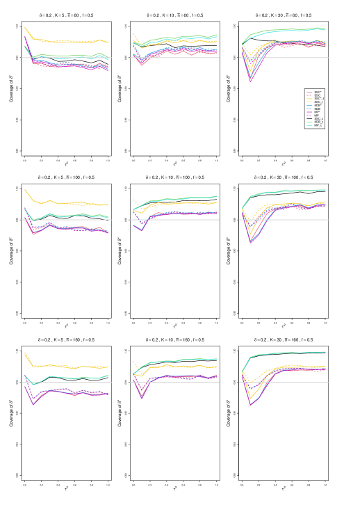
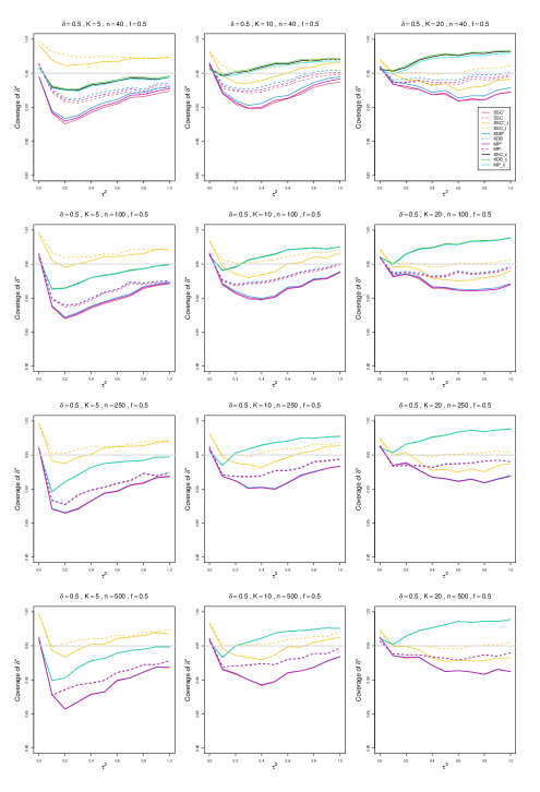
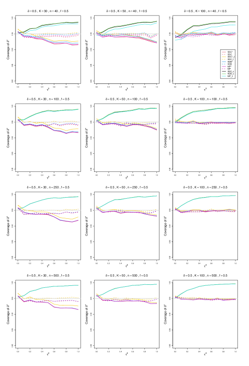
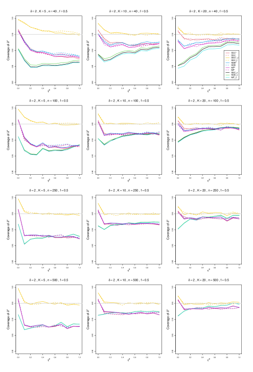
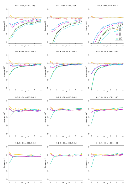
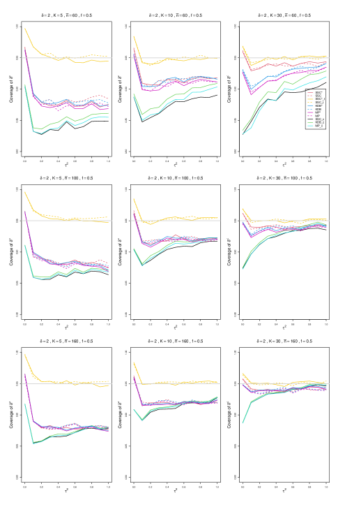
8.4 Coverage of naïve and corrected confidence intervals for based on signed SMD values, Appendix C
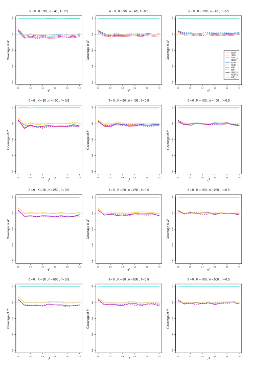
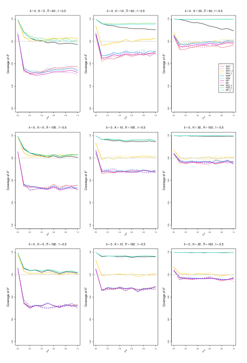
Coverage did not depend much on sample sizes. Confidence intervals based on normal critical values generally had low coverage for , especially for small and or , but their coverage improved with . There was no visible difference among the MP, KD, or SSC confidence intervals.
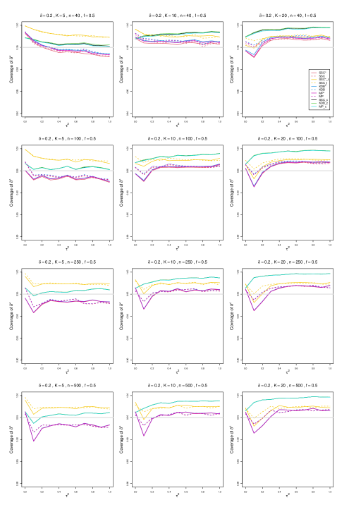
Naïve SSC_t confidence intervals, based on critical values, provided consistently good coverage for the vast majority of configurations. For or , their coverage was almost nominal for . For , coverage was above nominal when , but for it decreased to nominal for . Even for , coverage was somewhat above nominal for large values when .
For , there was almost no difference in coverage between normal- and t-based intervals.
We also studied coverage of the corrected confidence intervals. Coverage of the corrected SSC*_t confidence intervals was above 93.5% for all configurations, but it was typically below nominal for and , even for . Therefore, we do not recommend this correction.
8.5 Coverage of conditional confidence intervals for , Appendix C
When , coverage of the conditional confidence intervals follows from the above results on the empirical levels of the respective conditional tests. There was not much difference among the MP, KD, and SSC conditional confidence intervals, nor among sample sizes from to . For , coverage was near 1 when , it slowly decreased to nominal for larger . For , coverage decreased from 1 to about 98%, and for , coverage was near 1 for all values. However, for larger values of , coverage was near nominal when and then dropped dramatically for larger . This drop was more pronounced for and for larger . It was quite prominent when and but less so for and , where it was above nominal, but the drop was present even when and . Coverage then increased slowly with increasing , sometimes almost to nominal when . When , coverage was low for and increased slowly with .
9 Discussion
Though common in ecology and evolutionary biology, meta-analysis of magnitude effects has received little statistical attention, and the methods used so far are not appropriate. We formulate a random-effects model for meta-analysis of ASMD and propose appropriate statistical methods for point and interval estimation in meta-analysis of ASMD.
Statistical properties of squared SMD are more straightforward than those of its absolute value. Therefore, our methodological development focuses mainly on inference for . However, for inference on , one only needs to take the square root of the estimated and its confidence limits.
For point estimation of squared ASMD, we corrected an estimate of by subtracting the estimated between-study variance (in the signed SMD meta-analysis). Our simulations show that this works well when using a good estimator of such as MP, KD, or SSC.
For interval estimation, we considered three classes of statistical methods: naïve and corrected intervals for obtained from the signed SMD data and conditional methods based on the distribution of given the estimated . We found that coverage of the conditional confidence intervals was rather erratic, and the corrected confidence intervals provided somewhat low coverage in the vicinity of zero. However, naïve squaring of the SMD confidence limits, obtained with percentage points from the distribution, provided reliable coverage across all configurations of the parameters in our simulations and can be recommended for use in practice.
Acknowledgements
We are grateful to Prof Julia Koricheva who brought the meta-analysis of magnitude effects to our attention.
We would also like to thank Dr Michael Tsagris who kindly provided his simulation program for MLE estimation of parameters of the folded normal distribution used in Tsagris et al. [2014] and recommended the use of Rfast R package for this purpose.
The work by E. Kulinskaya was supported by the Economic and Social Research Council
[grant number ES/L011859/1].
References
- Ali et al. [2019] M Sanni Ali, Daniel Prieto-Alhambra, Luciane Cruz Lopes, Dandara Ramos, Nivea Bispo, Maria Y. Ichihara, Julia M. Pescarini, Elizabeth Williamson, Rosemeire L. Fiaccone, Mauricio L. Barreto, and Liam Smeeth. Propensity score methods in health technology assessment: Principles, extended applications, and recent advances. Frontiers in Pharmacology, 10(973), 2019. doi: 10.3389/fphar.2019.00973.
- Bailey et al. [2009] Joseph K. Bailey, Jennifer A. Schweitzer, Francisco Úbeda, Julia Koricheva, Carri J. LeRoy, Michael D. Madritch, Brian J. Rehill, Randy K. Bangert, Dylan G. Fischer, Gerard J. Allan, and Thomas G. Whitham. From genes to ecosystems: a synthesis of the effects of plant genetic factors across levels of organization. Philosophical Transactions of the Royal Society B: Biological Sciences, 364(1523):1607–1616, 2009. doi: 10.1098/rstb.2008.0336.
- Bakbergenuly et al. [2020] Ilyas Bakbergenuly, David C. Hoaglin, and Elena Kulinskaya. Estimation in meta-analyses of mean difference and standardized mean difference. Statistics in Medicine, 39(2):171–191, 2020. doi: 10.1002/sim.8422.
- Bakbergenuly et al. [2022] Ilyas Bakbergenuly, David C. Hoaglin, and Elena Kulinskaya. On the statistic with constant weights for standardized mean difference. British Journal of Mathematical and Statistical Psychology, 75(3):444–465, 2022. doi: 10.1111/bmsp.12263.
- Champagne et al. [2016] Emilie Champagne, Jean-Pierre Tremblay, and Steeve D. Côté. Spatial extent of neighboring plants influences the strength of associational effects on mammal herbivory. Ecosphere, 7(6):e01371, 2016. doi: 10.1002/ecs2.1371.
- Clements et al. [2022] Jeff C. Clements, Josefin Sundin, Timothy D. Clark, and Fredrik Jutfelt. Meta-analysis reveals an extreme “decline effect” in the impacts of ocean acidification on fish behavior. PLoS Biology, 20(2):e3001511, 02 2022. doi: 10.1371/journal.pbio.3001511.
- Costantini [2018] David Costantini. Meta-analysis reveals that reproductive strategies are associated with sexual differences in oxidative balance across vertebrates. Current Zoology, 64(1):1–11, 2018. doi: 10.1093/cz/zox002.
- DerSimonian and Kacker [2007] Rebecca DerSimonian and Raghu Kacker. Random-effects model for meta-analysis of clinical trials: an update. Contemporary Clinical Trials, 28(2):105–114, 2007. doi: 10.1016/j.cct.2006.04.004.
- Felix et al. [2023] Juri A. Felix, Philip C. Stevenson, and Julia Koricheva. Plant neighbourhood diversity effects on leaf traits: A meta-analysis. Functional Ecology, in press, 2023. doi: 10.1111/1365-2435……
- Garamszegi [2006] László Zsolt Garamszegi. Comparing effect sizes across variables: generalization without the need for Bonferroni correction. Behavioral Ecology, 17(4):682–687, 2006. doi: 10.1093/beheco/ark005.
- Gelman [2006] Andrew Gelman. Prior distributions for variance parameters in hierarchical models (comment on article by Browne and Draper). Bayesian Analysis, 1(3):515–534, 2006. doi: 10.1214/06-BA117A.
- Hedges [1983] Larry V. Hedges. A random effects model for effect sizes. Psychological Bulletin, 93(2):388–395, 1983.
- Johnson et al. [1995] Norman L. Johnson, Samuel Kotz, and N. Balakrishnan. Continuous Univariate Distributions, Volume 2. John Wiley & Sons, New York, second edition, 1995.
- Jones and Marchand [2021] M. C. Jones and Éric Marchand. A (non-central) chi-squared mixture of non-central chi-squareds is (non-central) chi-squared and related results, corollaries and applications. Stat, 10(1):e398, 2021. doi: 10.1002/sta4.398.
- Kulinskaya et al. [2004] E. Kulinskaya, M. B. Dollinger, E. Knight, and H. Gao. A Welch-type test for homogeneity of contrasts under heteroscedasticity with application to meta-analysis. Statistics in Medicine, 23(23):3655–3670, 2004. doi: 10.1002/sim.1929.
- Kulinskaya et al. [2011] Elena Kulinskaya, Michael B. Dollinger, and Kirsten Bjørkestøl. Testing for homogeneity in meta-analysis I. The one-parameter case: standardized mean difference. Biometrics, 67(1):203–212, 2011. doi: 10.1111/j.1541-0420.2010.01442.x.
- Leone et al. [1961] F. C. Leone, L. S. Nelson, and R. B. Nottingham. The folded normal distribution. Technometrics, 3(4):543–550, 1961. doi: 10.1080/00401706.1961.10489974.
- Mandel and Paule [1970] John Mandel and Robert C. Paule. Interlaboratory evaluation of a material with unequal numbers of replicates. Analytical Chemistry, 42(11):1194–1197, 1970.
- Morrissey [2016] M. B. Morrissey. Meta-analysis of magnitudes, differences and variation in evolutionary parameters. Journal of Evolutionary Biology, 29(10):1882–1904, 2016. doi: 10.1111/jeb.12950.
- Psarakis and Panaretoes [1990] S. Psarakis and J. Panaretoes. The folded t distribution. Communication in Statistics–Theory and Methods, 19(7):2717–2734, 1990. doi: 10.1080/03610929008830342.
- Rubin [2001] D. B. Rubin. Using propensity scores to help design observational studies: Application to the tobacco litigation. Health Services & Outcomes Research Methodology, 2:169–188, 2001.
- Sánchez-Meca and Marín-Martínez [2000] Julio Sánchez-Meca and Fulgencio Marín-Martínez. Testing the significance of a common risk difference in meta-analysis. Computational Statistics & Data Analysis, 33(3):299–313, 2000.
- Steiger [2004] James H. Steiger. Beyond the F test: Effect size confidence intervals and tests of close fit in the analysis of variance and contrast analysis. Psychological Methods, 9(2):164–182, 2004. doi: 10.1037/1082-989X.9.2.164.
- Tsagris et al. [2014] M. Tsagris, C. Beneki, and H. Hassani. On the folded normal distribution. Mathematics, 2(10):12–28, 2014. doi: 10.3390/math2010012.
Appendices
-
•
Appendix A: Bias in point estimation of
-
•
Appendix B: Empirical level of conditional tests of at 5% nominal level
-
•
Appendix C: Coverage of 95% confidence intervals for
Appendix A: Bias in point estimation of
Each figure corresponds to a value of the standardized mean difference (=0, 0.2, 0.5, 1, 2) and one of three combinations of or and a set of values of : {40, 100, 250, 500} and {5, 10, 20}, {40, 100, 250, 500} and {30, 50, 100}, {60, 100, 160} and {5, 10, 20}. The fraction of each study’s sample size in the Control arm () is held constant at 0.5.
For each combination of a value of (= 40, 100, 250, 500) or (= 60, 100, 160) and a value of (= 5, 10, 20 or 30, 50, 100), a panel plots bias versus (= 0(0.1)1).
The point estimators of are
-
•
KDB (Kulinskaya-Dollinger-Bjørkestøl) method, inverse-variance weights
-
•
MP (Mandel-Paule) method, inverse-variance weights
-
•
SSC method, effective-sample-size weights
For each method we include both truncated and non-truncated versions.
Appendix B: Empirical level of conditional tests of at a 5% nominal level
Each figure corresponds to the standardized mean difference . The fraction of each study’s sample size in the Control arm () is held constant at 0.5.
For each combination of a value of (= 40, 100, 250, 500) or (= 60, 100, 160) and a value of (= 5, 10, 20 or 30, 50, 100), a panel plots levels of conditional (given ) tests of versus (= 0(0.1)1).
The tests are
-
•
KDB, conditional test given (Kulinskaya-Dollinger-Bjørkestøl method), approximation
-
•
MP, conditional test given (Mandel-Paule method), approximation
-
•
SSC, conditional test given , approximation
-
•
KDB_b, conditional test given (Kulinskaya-Dollinger-Bjørkestøl method), bootstrap p-value, B=100000
-
•
MP_b, conditional test given (Mandel-Paule method), bootstrap p-value, B=100000
-
•
SSC_b, conditional test given , bootstrap p-value, B=100000
-
•
, a comparator test using known value, bootstrap p-value, B=100000
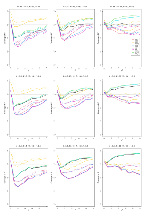
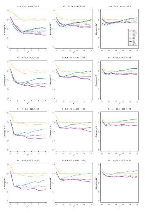
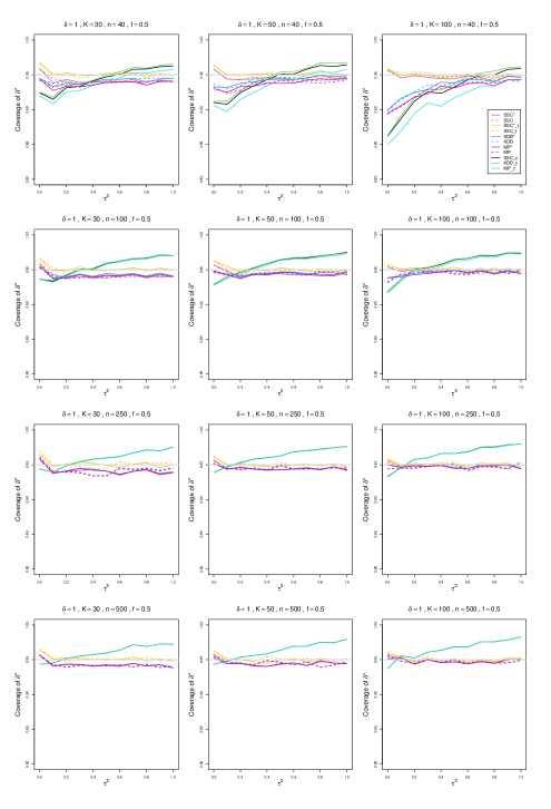
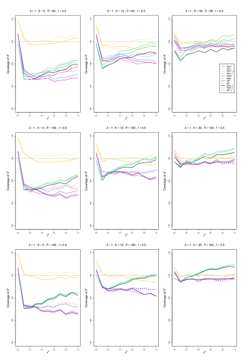
Appendix C: Coverage of 95% confidence intervals for
Each figure corresponds to a value of the standardized mean difference (=0, 0.2, 0.5, 1, 2). The fraction of each study’s sample size in the Control arm () is held constant at 0.5.
For each combination of a value of {40, 100, 250, 500} or {60, 100, 160} and a value of {5, 10, 20 or 30, 50, 100}, a panel plots coverage of versus (= 0(0.1)1).
The interval estimators of are
-
•
KDB (Kulinskaya-Dollinger-Bjørkestøl) method, inverse-variance weights, normal quantiles, based on the unsigned SMD values
-
•
MP (Mandel-Paule) method, inverse-variance weights, normal quantiles, based on the signed SMD values
-
•
SSC method, effective-sample-size weights, normal quantiles, based on the signed SMD values
-
•
SSC_t method, effective-sample-size weights, quantiles, based on the signed SMD values
-
•
KDB_c, conditional interval given (Kulinskaya-Dollinger-Bjørkestøl) method
-
•
MP_c, conditional interval given (Mandel-Paule method)
-
•
SSC_c conditional interval given
Unconditional intervals have two versions: a naïve version using confidence intervals or where is a CI for , (dashed lines) and a corrected version, denoted by * (straight lines). See text for details.