Covariance Expressions for Multi-Fidelity Sampling with Multi-Output, Multi-Statistic Estimators: Application to Approximate Control Variates ††thanks: This work was funded by the NASA Project: Entry Systems Modeling under grant no. 80NSSC22K1007.
Abstract
We provide a collection of results on covariance expressions between Monte Carlo based multi-output mean, variance, and Sobol main effect variance estimators from an ensemble of models. These covariances can be used within multi-fidelity uncertainty quantification strategies that seek to reduce the estimator variance of high-fidelity Monte Carlo estimators with an ensemble of low-fidelity models. Such covariance expressions are required within approaches like the approximate control variate and multi-level best linear unbiased estimator. While the literature provides these expressions for some single-output cases such as mean and variance, our results are relevant to both multiple function outputs and multiple statistics across any sampling strategy. Following the description of these results, we use them within an approximate control variate scheme to show that leveraging multiple outputs can dramatically reduce estimator variance compared to single-output approaches. Synthetic examples are used to highlight the effects of optimal sample allocation and pilot sample estimation. A flight-trajectory simulation of entry, descent, and landing is used to demonstrate multi-output estimation in practical applications.
Keywords uncertainty quantification multifidelity approximate control variate Monte Carlo estimation sensitivity analysis
1 Introduction
Estimating statistics of simulation models is of primary concern in uncertainty quantification. However, sampling strategies for estimation are often plagued by slow convergence. For example, the variance of a Monte Carlo (MC) mean estimator is proportional to the inverse of the number of model evaluations, requiring an order of magnitude more samples per digit of accuracy. As a result, the large number of sample evaluations required for accurate estimation becomes prohibitive when the underlying model is computationally burdensome. In this paper, we consider variance reduction techniques that reduce this cost by leveraging ensembles of correlated multi-output models for multiple statistics at once.
We focus on multi-fidelity sampling strategies that extract information from models of varying fidelities to reduce the variance of a baseline estimator without introducing bias. These lower fidelity models can take a hierarchical form, for example arising from a hierarchy of discretizations of a finite-element PDE approximation [2, 14], or they may be unstructured and include simulations with different physics and/or surrogates [26, 24]. In the context of multi-fidelity variance reduction, we focus on control-variate (CV) methods [12, 13, 21]. Examples of CV methods include the multi-level MC (MLMC) estimator [8, 2]; the multi-fidelity MC (MFMC) [17], and more generally appproximate control variates (ACV) [9]. While MLMC and MFMC require a distinct sampling structure of the ensemble of models, potentially limiting achievable variance reduction, the ACV method provides a general framework for distributing samples amongst models. More recently, the multi-level best linear unbiased estimator (MLBLUE) provides an alternate method to allocate samples based on estimator and model groupings [22], but can also be interpreted under the ACV framework.
Effectively leveraging multiple fidelities of models requires knowledge of the covariance between all models involved. As such, all of the above approaches require the prior knowledge of the covariance between the ensemble of high and low-fidelity estimators. These estimator covariances are intimately tied to the statistics being estimated. A majority of the literature focuses on mean estimation of scalar-valued functions [13, 12, 9, 3, 17, 8]. Some works on other statistics such as the variance [19, 20, 6], Sobol indices [19, 11, 20], and quantiles [10], also exist, but focus on single-statistic estimators. Note that MLMC does not require estimator covariances by making the strong assumption of perfect correlation amongst models, and, as a result, can yield sub-optimal choices of CV weights when the models are not perfectly correlated [9].
In the case of mean estimation, the covariance between MC estimators of each model is easily related to the covariances of the underlying models themselves [9, 3]. In practice, these model covariances are generally unknown, but estimated via some pilot sampling procedure. Pilot sample estimation can be performed with a fixed number of samples or through more adaptive or robust schemes. For example, an exploration-exploitation approach can be taken to minimize the total cost of model evaluations by determining when to stop estimating the model covariances [26]. Another approach directly estimates the covariance of the estimators by creating an ensemble of ACV estimators, each with a different set of samples [18]. For other statistics, such as probablility, quantile, or Sobol index estimation, the covariance between estimators is generally unavailable [19, 10, 11, 20]. For variance and Sobol index estimation, [19] finds the optimal weights for mean estimation and applies them to high-order statistic estimation. In [11], perfect correlation between estimators is assumed for Sobol index estimation, disregarding the estimator covariance requirement, but resulting in sub-optimal CV estimation. Finally, [20] numerically estimates the covariance between estimators directly for variance and Sobol indices to find the optimal CV weights. One of the principal aims of this paper is to introduce the analytic covariances for these additional estimators to improve CV efficiency.
A second issue that we consider is models with multiple outputs — the majority of the above approaches are applied to models with single outputs. Extending these approaches to vector-valued functions requires additional covariance expressions. Current state-of-the-art estimation techniques that use multiple quantities of interest (QoIs) construct one estimator for each QoI [24, 20, 5, 6]. While creating individual estimators is a simple technique, the correlations between the QoIs are lost, which leads to limited variance reduction. Indeed, in the context of classical CVs, Rubinstein and Marcus [21] show that the correlation between model outputs can be extracted by including vector-valued functions in a single estimator to further reduce the estimator variance. We extend these results to the ACV context. Additionally, estimating multiple statistics in a single estimator can lead to further sources of correlation, which can be extracted to reduce the variance of both statistics’ estimators. We newly introduce approaches to leverage multi-statistic information here.
In the context of multi-output mean estimation, a recent approach using the MLBLUE estimator was introduced to indeed extract model output correlations for vector-valued mean estimation [6]. A covariance matrix estimation approach was also introduced, but lacked the capability of extracting correlations between model outputs in this case. Similarly to [5], independent MLBLUE estimators were stacked into a matrix for vector-valued estimation. The approaches in this paper are applicable to further extending these MLBLUE results to take advantage of the correlations between model outputs for covariance matrix estimation. Similarly, this work introduces multi-statistic estimators for mean, variance, and Sobol indices which can further be applied to MLBLUE estimation.
We now summarize our contributions. First, we derive estimator covariances for multiple statistics and vector-valued functions for several important cases of interest that can be utilized in the majority of multi-fidelity sampling strategies. Propositions 3.1 and 3.4 provide the covariance between mean estimators and variance estimators, respectively, for vector-valued functions. Proposition 3.7 provides the covariance between the mean and variance estimators for simultaneous mean and variance estimation.
Second, we derive estimator covariances for all the main effect variances of scalar-valued functions for use in Sobol indices for global sensitivity analysis. The covariance between main effect variance estimators of similar/different indices is seen in Proposition 3.10. Similarly, Proposition 3.13 provides the covariance between the variance and main effect variance estimators since the total variance of the model is required for Sobol index estimation. These covariances allow multiple Sobol indices to be estimated simultaneously, providing a thorough sensitivity analysis across multiple inputs.
Finally, while these results can be adapted to several schemes, we utilize them to introduce the multi-output ACV (MOACV) estimator. This estimator can simultaneously estimate multiple statistics for vector-valued functions. We provide a number of empirical results that demonstrate that the MOACV estimator outperforms individual ACV estimators. As part of these results, we demonstrate that the newly derived estimator covariances for mean estimation do not require substantially more pilot samples than traditional ACV estimation. Finally, the MOACV estimator is tested on a realistic application of trajectory estimation for entry, descent, and landing (EDL) . The numerical results demonstrate significant further variance reduction compared to existing results.
The rest of this paper is structured as follows. Section 2 introduces MC sampling and the multi-output ACV theory. Section 3 provides the introduced estimator covariances and how to apply them to the ACV techniques. The results in Section 4 demonstrate the MOACV capabilities on analytical examples. Finally, Section 5 applies the MOACV estimator to the EDL application.
2 Background
In this section, we introduce notation, the core sampling-based estimators, and multi-fidelity variance reduction approaches.
2.1 Notation
The following notation is used throughout the manuscript. Matrices and vectors are denoted by bold-faced Roman letters. Each element of a matrix is denoted as for . Similarly each element of a vector is denoted by for . We denote a matrix of ones with size as . Generally, block matrices use an underline to denote that the block structure is important. If is an block matrix, then its blocks are denoted by
The Kronecker product between vectors is treated as a flattened outer product The element-wise product between two vectors or matrices is written as . The square of these two operations uses the following shorthand for both vectors and matrices and , respectively. Sets are denoted via upper case calligraphic letters such as
2.2 Monte Carlo Estimators
The -sample MC estimator of the mean of a function is defined using a set of input samples by
| (1) |
This estimator is unbiased and has variance . MC estimators can also be defined for the covariance
| (2) |
where , is a flattened estimate of the covariance matrix. Its variance is
| (3) |
and follows from Proposition 3.4.
Finally, we consider MC estimators for main effect Sobol sensitivity indices. To this end, the ANOVA decomposition [1] of the variance of a scalar-valued function is
| (4) |
where and is the -th input variable. The ANOVA decomposition separates the variance into terms attributed to the function’s inputs. One sensitivity measure is the global sensitivity index, or Sobol index [23], which is the percentage of variance attributed to the corresponding term of the ANOVA decomposition.
In this paper, we focus on the main effect sensitivity indices The Sobol estimator for the main effect can be obtained using two sets of input samples: , and , where is an independent set of input samples except for the th input, i.e., for . Using these sample sets the estimator for is
| (5) |
These estimators have a bias of [16], but are used for their simplicity. The variance of the Sobol estimator is
| (6) |
where , and . In the operation , the domain is independent from with the exception of the th input. For example, let and such that and share the same -th input. Thus, and are realizations of and respectively. To the best of our knowledge, Equation (6) is introduced in this paper and follows from Proposition 3.10.
2.3 Multi-Output Control Variates
The estimator variances described above all decrease at a rate of , which is prohibitive for expensive function evaluations. Variance reduction methods reduce this expense. CV approaches reduce variance by leveraging additional estimators with known statistics [13].
Let be an arbitrary estimator, and let denote a second random vector with known mean . The CV estimator is defined by
| (7) |
where is a matrix of weights and . This new estimator , has the same mean as . Furthermore, its variance is
| (8) |
The weights can be chosen to minimize some scalar-valued measure of the uncertainty represented by this variance. Rubinstein and Marcus [21] minimize the determinant, yielding111During vector-valued variance estimation, becomes singular due to duplicate columns from upper-lower triangular covariance pairs. To avoid the troubles of inversion, the pseudo-inverse can be used, or the upper triangular portion of the variance estimator can be isolated to provide a non-singular .
| (9) |
The determinant of the variance can be written as where are the canonical correlations between and [21]. Clearly, greater (anti)-correlations yield greater reductions in variance.
In the context of estimating statistics of computational models, the random variables and are the estimators using high- and low-fidelity models, respectively. In the uncertainty quantification problem, typically arises from an ensemble of lower-fidelity estimators according to222In this work, we assume for simplicity that all models share the same number of outputs. This assumption, however, can easily be disregarded by changing the shapes of the defined covariance matrices. The theory and results that follow can be easily modified to allow for varying quantities of model outputs.
| (10) |
2.4 Multi-Output Approximate Control Variates
In the UQ setting, are unknown. One approach to overcome this issue is to introduce new estimators for these terms and form an approximate control variate (ACV) [9]. The ACV estimators have only been defined in the scalar-function context, but we extend them here to vector-valued estimators by following the same ideas as in Section 2.3:
| (11) | ||||
| (12) |
where we now have potentially sample sets and have redefined . If and have the same expectation for all , the resulting estimator has the same bias as We denote the sample sizes associated with and to be and , respectively. Furthermore, these sets of samples may have a non-empty intersection denoted by subscripts with indices, for example, is the number of samples that are shared by and .
The expressions for the optimal weights and the variance in Equation (9) still apply to the ACV estimator using the new definition of .
3 Estimator Covariance Expressions
In this section, we provide a collection of results for the covariance between several estimators that are needed for many multi-fidelity sampling strategies. These estimator covariances can then be used within multifidelity UQ sampling approaches for considering multiple outputs and/or for systems needing multiple statistics. Specifically for ACVs, the covariance expressions are needed for evaluating and Section 3.1 summarizes how to find and for any estimator and sets up the following sections. Section 3.2 introduces estimators for the mean and covariance of multi-fidelity vector-valued functions. Section 3.3 introduces estimators for the simultaneous estimation of variance and main effects in the context of scalar-valued functions.
3.1 Setup and Summary
In this section, we describe the structure of the results that follow. Since is a vector of stacked estimators, the variance, , can be separated into a set of block covariance matrices:
| (13) |
Define , and further decompose each covariance block into
| (14) |
Lastly, the covariance with the high fidelity estimator is separated into
| (15) |
where
| (16) |
The subsequent sections derive expressions for the block components of these estimators, which can then be assembled into the final form. A summary of the estimator settings we consider and references to the results is provided in Table 1. For each case, the covariance between the required estimators of two fidelities and is first computed for arbitrary input sample sets and , where and . Here, let be the intersection between two input sample sets such that denotes the size of .
The computation of these components require certain statistics of the underlying multi-fidelity functions. To this end, subsequent sections begin with a highlighted box that describes what exactly is needed. In practice, these statistics can be available either analytically for some problems or must be obtained from pilot samples. Later, we numerically show that pilot samples are feasible in Section 4.2.
| MOACV Estimators | Propositions | |||||
|---|---|---|---|---|---|---|
| Estimators | Abbr. | Statistic | Model Output | |||
| Mean | M | Single | Multiple | 3.1 | 3.2 | 3.3 |
| Variance | V | Single | Multiple | 3.4 | 3.5 | 3.6 |
| Mean & Variance | MV | Multiple | Multiple | 3.7 | 3.8 | 3.9 |
| Main Effect Variances | ME | Multiple | Single | 3.10 | 3.11 | 3.12 |
| ME & Variance | MEV | Multiple | Single | 3.13 | 3.14 | 3.15 |
3.2 Mean and Variance Estimation
In this section, we estimate the mean and variance of a vector-valued function. In Section 3.2.1 and Section 3.2.2 we separately estimate the means and covariance, respectively. Finally, in Section 3.2.3 we simultaneously estimate the mean and covariance for vector-valued functions.
We further define notation for this section. Let , and be vector-valued functions collecting the outputs of a high-fidelity model and low-fidelity models according to
| (17) |
3.2.1 Mean Estimator
We now estimate the mean of a vector-valued function.
Proposition 3.1 (Covariance between Mean Estimators).
The covariance of two MC mean estimators (1), and , corresponding to fidelities computed via input sets , respectively, is
Proof.
Using the definition of covariance, we obtain
The function outputs are only correlated if the sampled inputs are the same. Thus, each covariance term is only nonzero if . The only nonzero covariance terms are due to samples in . Thus, there are nonzero covariance terms, and the stated result follows
| (19) |
∎
Using this result, we obtain the covariance between the discrepancies as follows333In this result, and those that follow, when , the equation simplifies greatly. Here it becomes . All other matrices defined similarly have a reduced form along the diagonals..
Proposition 3.2 (Variance of discrepancies for M).
The covariance between discrepancies is where
| (20) |
for and the starred quantities are defined in Section 2.4.
Proof.
The result follows a straightforward calculation
| (21) | ||||
∎
Note that when , Proposition 3.2 is equivalent to [3, Eq. 13]. Finally, the covariance between the high-fidelity and discrepancy estimators is provided. A similar argument yields the following result.
Proposition 3.3 (Variance between high-fidelity and discrepancies for M).
The covariance between the high-fidelity and discrepancy estimator is where
| (22) |
3.2.2 Variance Estimator
We now estimate the variance of a vector-valued function. The proofs are provided in the Appendix for brevity.
Proposition 3.4 (Covariance between Variance Estimators).
The covariance between two MC variance estimators (2), and , corresponding to fidelities computed via input sets , respectively, is
| (26) |
Using this result, we obtain the covariance between the discrepancies as follows.
Proposition 3.5 (Variance of discrepancies for V).
Let be the same as in Equation (20). The covariance between discrepancies is where
| (27) |
Finally, the covariance between the high-fidelity and discrepancy estimators is provided.
Proposition 3.6 (Variance between high-fidelity and discrepancies for V).
Let be the same as in Equation (22). The covariance between the high-fidelity and discrepancy estimator is where
| (28) |
3.2.3 Mean and Variance Estimators
We now consider a combined estimator, simultaneously providing a mean and variance (MV) estimate.
The stacked MC mean and variance estimator is
| (29) |
Proposition 3.7 (Covariance between Mean and Variance Estimators).
Using this result, we obtain the covariance between the discrepancies as follows.
Proposition 3.8 (Variance of discrepancies for MV).
Finally, the covariance between the high-fidelity and discrepancy estimators is provided.
3.3 Sensitivity Analysis
In this section, we estimate the covariances required for main effect (ME) Sobol indices of a scalar function. In Section 3.3.1, multiple ME variances are estimated simultaneously for a scalar function. In Section 3.3.2, the variance and multiple ME variances are estimated simultaneously.
For notation in this section, let and
| (33) |
where is the -th fidelity function with fixed -th input. Refer to discussion of Equation (6) in Section 2.2 for further details.
3.3.1 Main Effect Variance Estimators
We now estimate multiple ME variances of a scalar function. The combined ME variance estimator is
| (36) |
Proposition 3.10 (Covariance between Main Effect Variance Estimators).
The covariance between two stacked MC estimators (36), and , corresponding to fidelities computed via input sets , respectively, is
| (37) |
Using this result, we obtain the covariance between the discrepancies as follows.
Proposition 3.11 (Var. of discrepancies for ME).
The covariance between discrepancies is where
| (38) | ||||
| (39) | ||||
| (40) | ||||
| (41) |
Finally, the covariance between the high-fidelity and discrepancy estimators is provided.
Proposition 3.12 (Variance between high-fidelity and discrepancies for ME).
The covariance between the high-fidelity and discrepancy estimator is
where and
| (42) | ||||
| (43) | ||||
| (44) | ||||
| (45) |
3.3.2 Variance and Main Effect Variance Estimator
We now estimate the variance and multiple ME variances (MEV estimator) of a scalar function. The stacked variance and ME variance estimator is
| (46) |
Proposition 3.13 (Covariance between Variance and Main Effect Variance Estimators).
The covariance between two stacked MC estimators (46), and , corresponding to fidelities computed via input sets , respectively, is
| (47) |
where The diagonal terms of this block-matrix can be found in Propositions 3.4 and 3.10. Now, the covariance between the ME variance estimator and the variance estimator is
| (48) |
where is the first column of .
Using this result, we obtain the covariance between the discrepancies as follows.
Proposition 3.14 (Variance of discrepancies for MEV).
Finally, the covariance between the high-fidelity and discrepancy estimators is provided.
Proposition 3.15 (Variance between high-fidelity and discrepancies for MEV).
Remark 1.
The Sobol estimator can also apply to other effects, not just the ME. We can let multiple indices of interest in be dependent on , and estimate a combined effect variance. For example, in the ANOVA decomposition, we can estimate using the ME variance estimator, and thus, the same MOACV estimator as introduced above can be used. Therefore, the MOACV Sobol estimator is not restricted to only ME variance, and other variance terms in the ANOVA decomposition can be calculated.
4 Synthetic Numerical Examples
In this section, the performance of the multi-output estimator is investigated on synthetic vector-valued functions. In Section 4.1, the variance of the introduced multi-output estimator is compared to individual ACV estimation, and superior performance is shown. Section 4.2 explores the estimator performance when the required pilot covariances (given in the blue boxes of Section 3) are estimated. Generally, we find that as the number of estimated outputs are increased, more pilot samples are required if the pilot covariances are unknown. Moreover, higher order statistics, such as the ME variance, also can require significantly more samples.
The optimal sample allocations for the examples below are found by minimizing the determinant of the estimator variance subject to cost constraints
| (59) |
This formulation is consistent with both determinant minimization used for optimal weight determination in (9), and variance minimization in the single ACV case. Since the covariances and are functions of the number of estimator samples (, , , etc.), the required preliminary covariances are used to find the optimal sample allocation. Optimal allocations are found using the MXMCPy library444https://github.com/nasa/MXMCPy [4] for mean ACV and single-statistic MOACV estimators. Since MXMCPy does not offer optimization for variance estimation, the Scipy optimization library555https://docs.scipy.org/doc/scipy/reference/optimize.html is used for variance estimators.
The procedure in Section 4 and Section 5 estimates variance matrices. Traditional CV estimation of covariance matrices, however, may suffer from losing positive-definiteness [15], which leads to negative variance estimates. In these cases, any negative variance estimate in the following sections is set to zero. Next, the results in the following sections consider variance reduction, defined as the variance of a MC estimator divided by the variance of a multi-fidelity estimator. Finally, we use the following acronyms in the following sections. An MOACV estimator that estimates a single statistic, such as the mean or variance, is denoted as single MOACV (S-MOACV). An MOACV estimator that estimates multiple statistics is denoted as combined MOACV (C-MOACV).
4.1 Comparison to ACV Estimators
The variance reduction of MOACV estimators and individual ACV estimators is compared in this section. Consider a system with three models of decreasing fidelity, each with one input and three outputs
| (60) | ||||
| (61) | ||||
| (62) |
The endowed costs of each model are shown in Table 2. We assume perfect knowledge of the covariance between the models and their outputs. These correlations are shown in Figure 1, and are computed using 100,000 pilot samples. For demonstration purposes, all estimators follow the ACV-IS sampling scheme [9], we find that changing this scheme does not change the qualitative conclusions.
![[Uncaptioned image]](/html/2310.00125/assets/x1.png)
| Sample Allocations across Optimizations | ||||
|---|---|---|---|---|
| Model | Cost | ACV | S-MOACV | C-MOACV |
| Total Cost | ||||
4.1.1 Mean and Variance Estimation
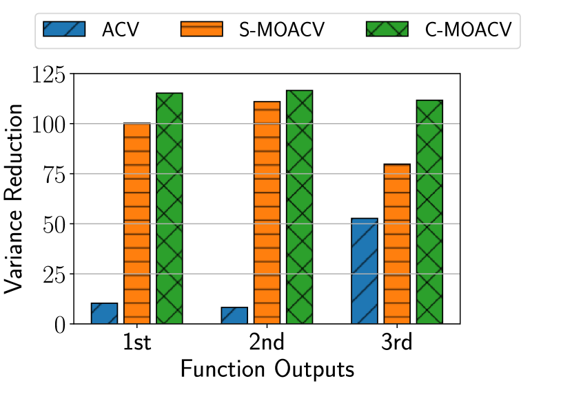
This section compares the variance reduction of individual ACV estimators with MOACV estimators for mean and variance estimation. To estimate the means and variances of each model output, the following estimators are constructed: six individual ACV estimators are constructed to estimate the three means and three variances; two S-MOACV estimators are constructed, one for the three means and one for the covariance matrix; and finally, a C-MOACV is created to simultaneously estimate the three means and the covariance matrix simultaneously. The same sample allocation is used for all estimators in this section, which is found by minimizing the variance of the ACV mean-estimator for the first output of given a budget of 10 seconds and is shown in the ACV column in Table 2. Note, the sample allocations shown in the other columns will be used in the subsequent sections.
Figures 2(a) and 2(b) display the variance reduction of the mean and variance estimators respectively. As seen in Figure 2(a), both the S-MOACV and C-MOACV estimators achieve greater variance reduction than the ACV estimator of each output by over an order of magnitude in some cases. C-MOACV also achieves improved variance reduction over the mean-specific S-MOACV. Figure 2(b) demonstrates similar results for the estimator variance, but indicates less benefit of C-MOACV over S-MOACV. The significantly improved variance reduction from S-MOACV estimation demonstrates that multi-output estimation excels in systems with the high correlations between the model outputs, as seen in Figure 1.

4.1.2 Sample Allocation Optimizations
In the previous section, all the estimators used the same sample allocation obtained from minimizing the variance of the mean ACV estimator for the first model output. In this section, performance of sample allocations that target variance reduction of the full multi-output estimator are demonstrated. The results in this section show variance reduction achieved only for the mean of the first model output, because that is all that the ACV can provide. We reinforce that the MOACV estimators also provide significant variance reduction for all other outputs as well.
Table 2 shows the optimal sample allocations for various objective functions. The first column, ACV, is the ACV-specific allocation for the first model output found in the previous section. The second (S-MOACV) and third (C-MOACV) columns arise from minimizing the determinant of the estimator variance obtained by the two MOACV estimators, respectively. While the optimization method resulted in sample allocations of slightly different costs666The different allocation costs is a consequence of simplifying the discrete optimization problem into a continuous domain. The rounding of the results of the continuous optimization into the discrete solution causes the solution to not lie on the computational budget boundary. However, the S-MOACV and ACV costs only have a 2% difference., the variance reduction metric is cost-independent since it divides the MC estimator variance by an equivalent-cost multi-fidelity estimator variance.
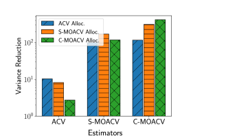
The variance reduction results are shown in Figure 3. Each of the optimizations give the best variance reduction for their respective estimators. For example, the C-MOACV estimator that uses a C-MOACV optimal sample allocation achieves more variance reduction than a C-MOACV estimator that uses the ACV optimal sample allocation. The C-MOACV estimator outperforms the ACV estimator by at least an order of magnitude under all allocation strategies. We reinforce that while variance reduction significantly improves for the mean of the first output, the combined MOACV estimator also returns the means, variances, and covariances of all other model outputs.
4.2 Pilot Sample Trade-off
The multi-output estimators introduced in this work require exploiting more information than simple single-output estimators. Specifically, the boxes of Section 3 show a large number of statistics that must be known to compute the optimal CV weights. A natural question arises as to whether there are too many unknowns to allow a small set of pilot samples to yield an effective estimate. In this section, it is shown that the required number of pilot samples depends on the number of model outputs and statistics that are estimated. The type of statistic estimated is the largest contributor to the number of pilot samples that is required, while adding more outputs gradually increases the number of required samples.
A new system is defined to consider a tunable number of function outputs to study convergence of increasingly complex estimators as a function of the number of pilot samples. Let the high- and low-fidelity functions be , where is uniformly distributed such that
| (63) |
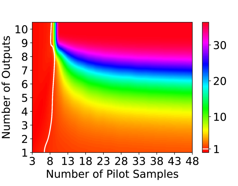
We will study the variance reduction in the mean and main-effect variances of the first output of . For mean estimation, we consider an increasing number of model outputs formed by using more components of each of the model fidelities. For ME variance estimation, we consider an increasing number of ME variances to estimate across the 9 inputs. The ACV-IS sampling scheme was chosen with the un-optimized allocations of each fidelity being , , and . Figure 4 shows the variance reduction achieved for different numbers of pilot samples and statistics. Note that the bottom edge of the plots corresponding to one output for mean estimation in Figure 4(a) and one ME in Figure 4(b) corresponds to the performance of the standard ACV estimator.
To determine the performance of the variance reduction with respect to the number of pilot samples, we sweep across combinations of additional model outputs (from 0 to 9) and numbers of pilot samples. At each pilot sample quantity, we run 1000 realizations of the pilot sample sets and compute the estimator variances. Figure 4(a) shows the 5th percentile of the variance reduction, a statistic that demonstrates close to worst-case behavior.
The white line corresponds to the variance reduction ratio of 1, where MC has equal performance to the CV approach. Notably, we see a sharp transition at 10 pilot samples where the performance improves over MC. With too few pilot samples, the estimators perform worse than MC. Since the white contour line is near vertical, Figure 4(a) displays that adding more correlated outputs in mean estimation only requires slightly more pilot samples for significantly improved variance reduction.
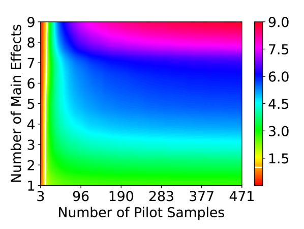
Next we repeat the same experiment for the ME variances of the first output of with respect to each of the 9 inputs. As described in Section 3.3, there are many more required covariances to be estimated for multiple ME estimators than for mean estimation. The statistic of interest is also of a higher order than mean estimation. Figure 4(b) again shows the 5th percentile of the variance reduction for the first ME variance output over the 1000 trials at different combinations of outputs. In this case, the number of outputs in the estimator reflects the number of MEs that are estimated, a maximum of 9 for the 9 total inputs. Note the different axis scales between the two plots. Similarly to mean estimation, the additional statistics can improve the variance reduction. However, the number of required pilot samples to outperform ACV (green area, bottom edge of Figure 4(b)), is about 25 samples, which is double the number of samples required for mean estimation. Further, the maximum variance reduction requires around 250 pilot samples before the C-MOACV estimator variance converges. Overall, we see a similar pattern to the mean estimation with more required samples. In both mean and ME estimation, the MOACV estimators achieve larger variance reduction than ACV estimation when the ACV estimator variance has converged. Future work can focus on adaptive schemes to determine the optimal number of pilot samples.
5 Application: Entry, Descent, and Landing Trajectories
Entry, descent, and landing (EDL) is the final phase of a space vehicle’s mission upon entering the atmosphere of a celestial body. An important aspect of successful EDL includes prediction of trajectory and touchdown properties including locations, velocities, and states of a vehicle at given times. However, these predictions are difficult because of uncertainties due to the atmosphere, initial vehicle states, and actuator precision. Analyzing predicted outcomes due to these uncertainties is also computationally challenging because high-fidelity simulations may take hours or days to run. In this section, we consider the simulation of a sounding rocket with the aim of reducing the computational cost of estimation through multi-fidelity methods.
NASA launched the Sounding Rocket One (SR-1) in September 2018 containing the Adaptable, Deployable, Entry, and Placement Technology (ADEPT), aimed to demonstrate a deployable aeroshell used for re-entry [7]. Before launch, this flight was simulated using the Program to Optimize Simulated Trajectories II (POST2) software [25] with a standard MC approach to consider system uncertainties [7]. The POST2 software contains around 75 uncertain inputs including initial conditions (e.g. location, velocity, angle of attack), vehicle parameters (e.g. moment of inertia, deployment impulse), and environmental parameters (e.g. atmospheric uncertainty). In Warner, et al. [24], ACV techniques were used to construct mean estimators for 15 trajectory QoIs, such as the touchdown latitude, longitude, velocity, and other QoIs listed in [24, Table 1]. Using multi-fidelity techniques, [24] was able to reduce the variance of estimation for many of the 15 QoIs. The goal of this section is demonstrate further variance reduction using multi-output estimation. The following models of varying fidelity were introduced in [24] to aid the multi-fidelity estimation. The POST2 simulation is used as the high-fidelity model which takes 219 seconds on average for a single evaluation at a fixed condition. A “reduced-physics” version of POST2 is introduced to reduce the cost of simulation by using a simplified atmospheric model, taking around 47.4 seconds per evaluation. A cheaper trajectory simulation is also created using the high-fidelity POST2 at a much larger integration time step at 2.8 seconds per evaluation, deemed the “coarse time-step” model. Finally, a support vector machine (SVM) surrogate model (“machine learning model”) is trained offline using 250 high-fidelity trajectory simulations and used as a low-fidelity model taking around 0.0007 seconds per evaluation.
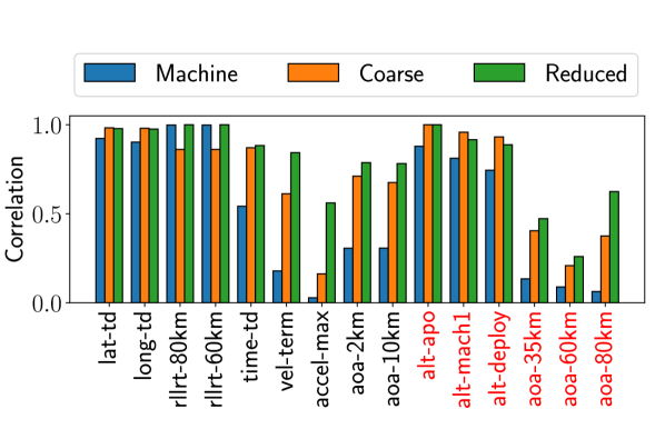
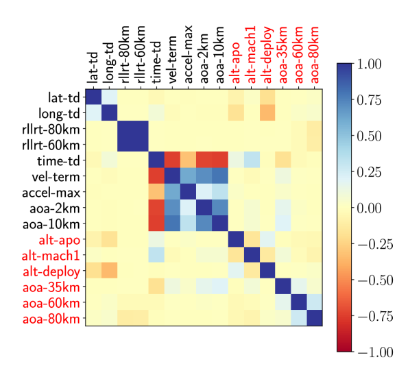
In this section, we compare the performance of multi-output methods to ACV estimation for 9 of the 15 QoIs. The 9 QoIs were chosen for their correlations between other QoIs, as seen in Figure 5(b), where the QoIs in red are removed from this study. Section 5.1 compares ACV and MOACV methods by estimating the mean and variance of 9 QoIs. Finally, Section 5.2 uses MOACV to perform a sensitivity analysis on one QoI across three input variables.
5.1 Mean and Variance Estimation
In this section, we build 18 ACV estimators for the mean and variance of each of the 9 QoIs; two S-MOACV estimators, one for 9 mean estimators and one for 9 variance estimators; and a single C-MOACV estimator for the mean and variance of the 9 QoIs simultaneously. In particular, the C-MOACV estimator simultaneously estimates 54 statistics (9 means and 45 unique covariances).
To find the preliminary covariances, 60,000 pilot samples were used. With these samples, Figure 5(a) shows the correlations between the models across the model outputs. Notably, a few QoIs have low correlations between the low-fidelity and high-fidelity models. Traditionally, poor variance reduction is expected at these QoIs for multi-fidelity estimation. The correlations between the outputs of the high fidelity model can be seen in Figure 5(b). The non-zero correlations are exploited in the MOACV techniques and used to provide more accurate estimation.
A single ACV-IS allocation scheme was applied to all outputs to enable a fair comparison at equivalent computational costs. This sample allocation for all estimators was computed to minimize the variance of the ACV mean-estimator for the touchdown latitude (lat-td). Similarly, to Warner et al. [24], the optimization minimizes the variance with a computational budget of seconds. The allocated samples are 31, 0, 1124, and 22075 samples for the POST2, reduced physics model, coarse time step model, and the machine learning model respectively.
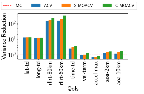
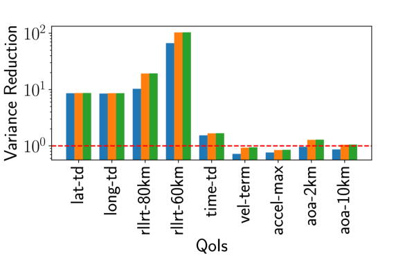
We obtain the empirical variance of the estimators using 10,000 realizations of data according to the above sample allocation. The variance reduction achieved for mean and variance estimation can be seen in Figure 6. The red dotted line represents no reduction compared to the equivalent-cost MC estimator. The individual ACV estimator reduction can be seen in the blue bars. In Figure 6(a) for mean estimation, the S-MOACV and C-MOACV achieves greater variance reduction than individual ACV estimation at every QoI. In Figure 6(b), both the S-MOACV and the C-MOACV estimators achieve greater variance reduction than the ACV estimator at every QoI.
Figure 6 demonstrates that the MOACV estimators can turn situations where an ACV estimator performed worse than MC, into one where performance becomes better than MC. For example, the ACV estimator for the terminal velocity “vel-term” initially performs worse than MC estimation. However, the C-MOACV estimator is able to achieve reduction better than MC by leveraging the additional correlations. For mean estimation, the S-MOACV estimator achieves a median 15% greater variance reduction than ACV estimators. The C-MOACV estimator achieves a median 39% larger variance reduction than ACV estimators, with a maximum of 113% larger reduction for “rllrt-60km”. For variance estimation, the C-MOACV estimator provides a median 22% greater variance reduction than ACV estimators. The C-MOACV estimates for landing latitude and longitude performed marginally better (about 1% larger reduction) than ACV estimation. This performance is explained by the lack of correlation amongst latitude and longitude with other QoIs, as seen in Figure 5(b). The S-MOACV and C-MOACV estimators are able to outperform traditional ACV methods by extracting the correlations between QoI and statistics to reduce the variance of ACV estimation even further.
5.2 Sensitivity Analysis
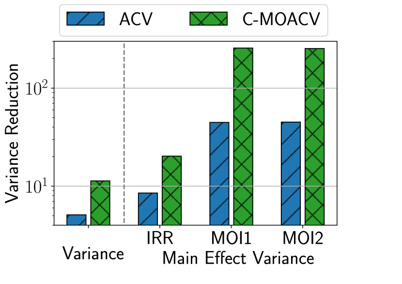
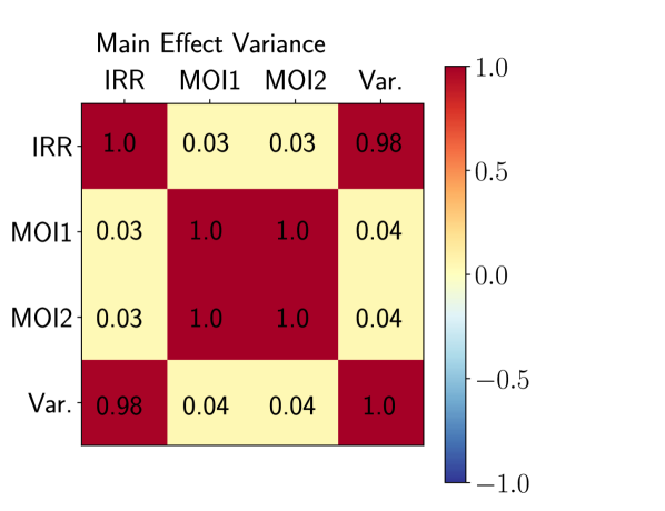
In this section, the C-MOACV estimator performs a sensitivity analysis on the roll rate at 80 km by simultaneously estimating the Sobol indices of three input variables, the initial roll rate (IRR) and two uncertainties in the vehicle’s moment of inertia, MOI1 and MOI2. The input variables and QoI were chosen to demonstrate the ME variance estimation for variables with both high and low Sobol indices. The C-MOACV estimator contains 4 outputs, the 3 ME variance estimators and 1 total variance () estimator. The Sobol indices are then constructed by dividing the ME variance estimate by the total variance estimate from the C-MOACV estimator. The preliminary covariances are estimated using 5,000 pilot samples. The C-MOACV and ACV estimators use the ACV-IS sampling scheme, and the sample allocation was found by minimizing (59) with the C-MOACV variance subject to a budget of 10,000 seconds. The sample allocation is 21, 99, 200, and 7359 samples for the full-physics, reduced-physics, coarse time-step, and machine learning models respectively.
Figure 7(a) shows the variance reduction compared to MC estimation for the individual ACV estimators and the C-MOACV estimator. The C-MOACV variance reduction is a median 300% larger than ACV estimation. Since the ME variance estimator is only defined for scalar functions, the C-MOACV estimator can only outperform the ACV estimator if there are large correlations between the MC ME variance and total variance estimators. In Figure 7(b), the correlations between 10,000 MC estimators for the variance and ME variance can be seen. Large correlations are shown between the ME variance estimates and the total variance estimates. The MOACV estimator is able to extract these high correlations to reduce the variance of each of the estimators.
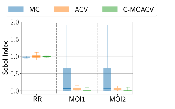
We now form the Sobol index estimates by dividing the ME variance estimate by the total variance estimate for the MC, ACV, and MOACV estimators. To measure the distribution of Sobol index estimates, 10,000 estimators are constructed with random realizations of input samples. The distribution of the 10,000 Sobol index estimates is seen in Figure 8(a). The Sobol index of IRR is around , and the MOI Sobol estimates are close to . Since a Sobol index is the percentage of the model’s variance for an input, almost 100% of the QoI’s (roll rate at 80 km) variance is attributed to the initial roll rate. This high percentage explains the high correlation between the IRR ME and the variance estimates seen in Figure 7(b). Conversely, the approximately 0% Sobol index of the MOIs explains the low correlation between their ME and total variance estimates.
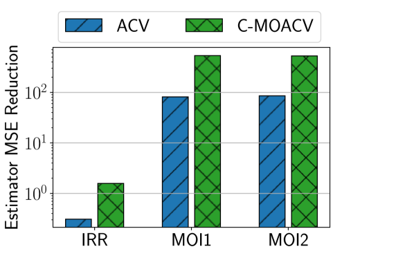
While Figure 8(a) displays the qualitative difference between ACV and C-MOACV Sobol index estimation, we now directly compare the error in each of the Sobol index estimates. Since the Sobol index estimates are found by dividing two estimators, the resulting Sobol index estimates are biased. Instead of measuring the variance of estimation, the mean squared error (MSE) is calculated to now consider the bias from the truth, which was calculated using 10,000 high-fidelity samples. The MSE for the MC estimates are divided by the MSE for the multi-fidelity estimates to calculate the MSE reduction. In Figure 8(b), the MSE reduction compared to MC estimation of the Sobol index estimates is seen. The C-MOACV estimator reduces the MSE in all Sobol index estimates compared to ACV estimation. The MSE reduction for the C-MOACV estimates is a median 515% greater than the MSE reduction for ACV estimates. This section validates that the MOACV estimator can be used for more accurate sensitivity analysis and provides an example that the MOACV estimator can achieve further variance reduction by using the correlation between estimators.
6 Conclusion
In this work, we have introduced closed-form expressions for the covariance between MC estimators of multi-output functions for a variety of statistics. We have also used these results in the ACV context to construct the multi-output ACV estimator. The introduced multi-fidelity estimators include the vector-valued mean and variance estimators that utilize the correlations between models, outputs, and estimators to improve variance reduction. For sensitivity analysis, the MOACV estimator is demonstrated to simultaneously estimate the variance and multiple ME variances for more accurate Sobol indices.
Numerous results demonstrate that the correlations between model fidelities, model outputs, and estimators can be extracted to provide further variance reduction. In the synthetic numerical results, the C-MOACV estimator is able to achieve up to 183 times larger variance reduction compared to a traditional ACV estimator. The MOACV estimator is also applied to an entry, descent, and landing application to more accurately estimate 9 QoIs given a fixed computational budget. Further, a variance-based sensitivity analysis is performed to illustrate the expected improved accuracy of the C-MOACV estimator. The C-MOACV estimator is able to increase the MSE reduction of Sobol index estimates by up to 557% compared to traditional ACV estimation. In summary, multi-output estimation techniques are able to significantly outperform traditional ACV methods when high correlations exist between model outputs and estimators.
In future work, the ME variance estimator can be extended to vector-valued functions. Since the variance estimator has already been defined for multiple outputs, the extension to the ME variance estimator will be able to take advantage of correlations between other model outputs. Extending the estimator to vector-valued functions would enable the sensitivity analysis to be performed on multiple model outputs and inputs simultaneously. Additionally, the introduced estimator covariances can be applied to other multi-fidelity sampling strategies, such as the MLBLUE estimator for multi-statistic estimation. New strategies can be introduced to find the optimal number of pilot samples that minimize the total model evaluation cost, such as multi-arm bandit learning approaches [26]. Finally, covariance estimation techniques can be used to mitigate the loss of positive-definiteness by estimating on a covariance manifold [15].
References
- [1] G. E. B. Archer, A. Saltelli, and I. M. Sobol. Sensitivity measures, anova-like techniques and the use of bootstrap. Journal of Statistical Computation and Simulation, 58:99–120, 1997.
- [2] Andrea Barth, Christoph Schwab, and Nathaniel Zollinger. Multi-level monte carlo finite element method for elliptic pdes with stochastic coefficients. Numerische Mathematik, 2011.
- [3] G. F. Bomarito, P. E. Leser, J. E. Warner, and W. P. Leser. On the optimization of approximate control variates with parametrically defined estimators. Journal of Computational Physics, 451, 2022.
- [4] G. F. Bomarito, J. E. Warner, P. E. Leser, W. P. Leser, and L. Morrill. Multi model monte carlo with python (mxmcpy). NASA/TM–2020–220585, 2020.
- [5] M. Croci, K. E. Willcox, and S. J. Wright. Multi-output multilevel best linear unbiased estimators via semidefinite programming. Cornell University Arxiv, 2023.
- [6] Mayeul Destouches, Paul Mycek, and Selime Gürol. Multivariate extensions of the multilevel best linear unbiased estimator for ensemble-variational data assimilation. Cornell University Arxiv, 2023.
- [7] Soumyo Dutta, Christopher D. Karlgaard, Ashley M. Korzun, Justin S. Green, Jake A. Tynis, Joseph D. Williams, Bryan Yount, Alan M. Cassell, and Paul F. Wercinski. Adaptable deployable entry and placement technology sounding rocket one modeling and reconstruction. Journal of Spacecraft and Rockets, 59(1), 2022.
- [8] Michael B. Giles. Multilevel monte carlo path simulation. Operations Research, 56(3):607–617, 2008.
- [9] Alex A. Gorodetsky, Gianluca Geraci, Michael S. Eldred, and John D. Jakeman. A generalized approximate control variate framework for multifidelity uncertainty quantification. Journal of Computational Physics, 408, 2020.
- [10] Timothy C. Hesterberg and Barry L. Nelson. Control variates for probability and quantile estimation. Institute for Operations Research and the Management Sciences, 44(9):1295–1312, 1998.
- [11] S. Kucherenko, B. Delpuech, B. Iooss, and S. Tarantola. Application of the control variate technique to estimation of total sensitivity indices. Reliability Engineering and System Safety, 134:251–259, 2015.
- [12] S. S. Lavenbcrg, T. L. Moeller, and P.D. Welch. Statistical results on multiple control variables with application io variance reduction in queueing network simulation. IBM Research Report RC 742, 1978.
- [13] S. S. Lavenberg and P. D. Welch. A perspective on the use of control variables to increase the efficiency of monte carlo simulations. Management Science, 27(3):322–335, 1981.
- [14] Yan Luo and Zhu Wang. A multilevel monte carlo ensemble scheme for random parabolic pdes. SIAM Journal on Scientific Computing, 41(1):A622–A642, 2019.
- [15] Aimee Maurais, Terrence Alsup, Benjamin Peherstorfer, and Youssef Marzouk. Multi-fidelity covariance estimation in the log-euclidean geometry. International Conference on Machine Learning, 2023.
- [16] Art B. Owen. Variance components and generalized sobol’ indices. Stanford University, 2012.
- [17] Benjamin Peherstorfer, Karen Willcox, and Max Gunzburger. Optimal model management for multifidelity monte carlo estimation. SIAM Journal on Scientific Computing, 38(5):A3163––A3194, 2016.
- [18] Trung Pham and Alex A. Gorodetsky. Ensemble approximate control variate estimators: Applications to multi-fidelity importance sampling. SIAM Journal of Uncertainty Quantification, 10(3):1250–1292, 2022.
- [19] E. Qian, B. Peherstorfer, D. O’Malley, V. V. Vesselinov, and K. Willcox. Multifidelity monte carlo estimation of variance and sensitivity indices. SIAM Uncertainty Quantification, 6(2):683–706, 2018.
- [20] A. Quaglino, S. Pezzuto, and R. Krause. High-dimensional and higher-order multifidelity monte carlo estimators. Journal of Computational Physics, 338(1):300–315, 2019.
- [21] Reuven Y. Rubinstein and Ruth Marcus. Efficiency of multivariate control variates in monte carlo simulation. Operations Research, 33(3):661–677, 1985.
- [22] Daniel Schaden and Elisabeth Ullmann. On multilevel best linear unbiased estimators. SIAM Journal of Uncertainty Quantification, 8(2):601–635, 2020.
- [23] I. M. Sobol. Global sensitivity indices for nonlinear mathematical models and their monte carlo estimates. Mathematics and Computers in Simulation, 55:271––280, 2001.
- [24] James E. Warner, Samantha C. Niemoeller, Luke Morrill, Geoffrey F. Bomarito, Patrick E. Leser, William P. Leser, Robert A. Williams, and Soumyo Dutta. Multi-model monte carlo estimators for trajectory simulation. AIAA SciTech Forum, 2021.
- [25] Robert A. Williams, Rafael A. Lugo, Steven M. Marsh, James A. Hoffman, Jeremy D. Shidner, and John T. Aguirre. Enabling thread safety and parallelism in the program to optimize simulated trajectories ii. American Institute of Aeronautics and Astronautics, 2023.
- [26] Yiming Xu, Vahid Keshavarzzadeh, Robert M. Kirby, and Akil Narayan. A bandit-learning approach to multifidelity approximation. SIAM Journal on Scientific Computing, 44(1):A150––A175, 2022.
Appendix A Three Useful Covariance Results
First, let be dependent random variables, and let be independent random variables with respect to all other random variables. By linearity of expectation,
Next, we wish to derive
| (A.1) |
Finally, another useful covariance is
| (W) | |||
| (X) | |||
| (Y) | |||
First, (X) is considered. Note that when . Now,
| (A.2) |
using Kronecker and Hadamard mixed product properties. Similarly,
| (A.3) |
Finally, consider (Z)
| (A.4) |
Therefore, by combining (W), (X), (Y), and (Z)
| (A.5) |
Appendix B Proof of Proposition 3.4
Here, the covariance between two variance estimators (2) is derived. For notation, let and , and
| (B.6) |
The covariance in the quadruple sum is zero when the input samples are not shared between fidelities (). Also, when , which means the covariance is similarly zero. The same is true when . We can break the rest of the nonzero terms of the quadruple sum into 6 cases that each correspond to different combinations of shared inputs. Let , , and . Thus
| (A) | ||||
| (B) | ||||
| (C) | ||||
| (D) | ||||
| (E) | ||||
| (F) |
Note that we abuse notation in the sum notation, , such that is an integer representing the input sample in . First, we simplify (A) by rewriting the covariance in terms of the underlying functions’ ( and ) statistics. We then note that the terms for (A) are the same as (B), (C), and (D) such that (A)=(B)=(C)=(D). Finally, we will simplify (E) and note that (E)=(F). First, consider the terms in (A) by expanding the Kronecker squares
| (B.7) |
Since are are independent of each other while are are dependent, we use Appendix A to introduce expectations. Further, the input samples are i.i.d. such that the expectations of can be rewritten as expectations of the underlying function . Finally, we factor the equation into a simplified form
| (B.8) | ||||
The same argument holds for (B), (C), and (D) simply by recognizing that and noting that the triple sums are equivalent. Thus, , and
| (B.9) |
Because the covariance terms are not dependent on the specific samples, we only need to tabulate how many times the covariance arises in the sum. To this end, note that the set can be partitioned as a disjoint union of four sets, , , , and . The cardinality of these sets are , , , and respectively. By adding the cardinalities together,
| (B.10) |
Now, we consider the covariance in term (E) by following the same procedure
| (G) | ||||
| (H) | ||||
| (I) | ||||
| (J) |
Again, note (G) and (H) are equivalent due to symmetry. Using Appendix A, we combine (G) and (H) using a similar process as (B.8)
| (B.11) |
Now, consider (I) and (J) and note that the second covariance inputs are identical. We now combine (I) and (J)
| (K) | ||||
| (L) | ||||
| (M) |
by separating the second covariance inputs. Since , we combine the terms in (K) by using Appendix A, Now, we consider (L) by breaking the covariance into expectations
The argument for (M) is identical with the following result
| (B.13) |
Now, we find in order to remove the dependence on and
| (B.14) |
using the Kronecker and Hadamard mixed-product properties. The argument for is identical such that (L)=(M).
Now, we rewrite (K) by adding and subtracting an additional term to facilitate simplification in later steps
Adding (K) to (G) and (H) yields
| (N) | ||||
| (O) |
Now, we break (O) into expectations
| (B.16) |
Now, we combine (O), (L), and (M), and use the results from Appendix A
Therefore, by combining (N), (O), (L), and (M), we obtain a final expression for (E)
The argument for the covariance term in (F) is identical, and their sums are equivalent such that . Now, we only need to tabulate how many times the covariance arises in the sum since the covariance is independent of specific samples. Thus, the set has the cardinality of . Therefore,
| (B.19) |
Combining coefficients yields our stated result
| (B.20) |
Appendix C Proof of Proposition 3.5 and 3.6
Now, Equation (B.20) is used to find the discrepancy covariances with different input samples
| (C.21) | ||||
| (C.22) |
Similarly to above, Equation (B.20) can be used with different input samples to find the covariance between the high-fidelity estimator and the discrepancy.
Appendix D Proof of Proposition 3.7, 3.8, and 3.9
We now find the covariance between the mean and variance estimators
| (D.23) |
We consider the 2 cases of shared input samples that relate to nonzero covariance terms
| (A) | |||
Note that (A) = (B) by the same argument from below Equation (B.8). Thus, consider (A)
| (D.24) |
using the results of Appendix A and the fact that the input samples are i.i.d. where the statistics can be rewritten in terms of the underlying functions’ statistics. The cardinality of the set is . Thus,
| (D.25) | ||||
| (D.26) |
Propositions 3.8 and 3.9 follow by using the above equation with different sets of input samples.
Appendix E Proof of Proposition 3.10, 3.11, and 3.12
We now find the covariance between two main effect variance estimators. Let and that follow the same sample partitioning described in Section 2.2. Now,
| (E.27) | ||||
| (E.28) |
There are 11 cases of nonzero covariance terms which are found through combinations of sharing input samples. We start with the case when . Using Appendix A and the fact that the samples are i.i.d. such that the statistics can be written in terms of the underlying functions’ statistics
| (E.29) |
This process is repeated for all combinations of sets of shared input samples. The results can be seen in Table 3,
| Shared Samples | Covariance | Occurrence Frequency |
|---|---|---|
| Eq. (E.30) | ||
| Eq. (E.31) | ||
The derivations for and are not as straightforward as the other results in the table. Thus, consider
| (E.30) | ||||
The final case to consider is when
| (E.31) |
To combine all of these cases together,
| (E.32) | ||||
Equation (LABEL:eq:me_result) is the covariance across two input variables, and . We now stack the covariances to include all input indices, , such that the covariances are matrices. Thus,
| (E.34) |
Propositions 3.11 and 3.12 follow by using the above equation with different sets of input samples.
Appendix F Proof of Proposition 3.13, 3.14, and 3.15
The covariance between the MC variance estimator and the main effect variance estimator is found
| (F.35) | ||||
| (F.36) |
We consider 8 cases that result in nonzero covariance terms which can be seen in Table 4,
| Shared Samples | Covariance | Occurrence Frequency |
|---|---|---|
| Eq. (F.38) | ||
| Eq. (F.38) |
Now, the following cases are not as straightforward as the results in the table. Consider
| (A) | ||||
Now, consider (B)
| (F.37) |
By combining (A) and (B),
| (F.38) |
We note here that the argument is the same for with an identical result. These results are then combined
Similarly, by taking its transpose,
| (F.40) |
Equation (F.40) defines the covariance for one input of interest. We now stack the covariances to include all input indices, ,
| (F.41) | ||||
| (F.42) |
where is the first column of . Now, Propositions 3.14 and 3.15 follow by using the above equations with different input sample sets.