Sensor Placement for Flapping Wing Model
Using Stochastic Observability Gramians

Abstract

Systems in nature are stochastic as well as nonlinear. In traditional applications, engineered filters aim to minimize the stochastic effects caused by process and measurement noise. Conversely, a previous study showed that the process noise can reveal the observability of a system that was initially categorized as unobservable when deterministic tools were used. In this paper, we develop a stochastic framework to explore observability analysis and sensor placement. This framework allows for direct studies of the effects of stochasticity on optimal sensor placement and selection to improve filter error covariance. Numerical results are presented for sensor selection that optimizes stochastic empirical observability in a bioinspired setting.

Keywords Observers for nonlinear systems  $\cdot$ Computational Methods  $\cdot$ Stochastic Systems

1 Introduction

Performance resilience in the presence of sensing noise, environmental disturbances, and modeling imprecision is typically approached from the perspective of robust control theory. However, all feedback-based control techniques, including robust methods, are constrained by the quality of the state estimate as determined both by the accuracy of the estimate (how close the estimate is to the true value) and the precision (how well the estimate is known). Specifically, the precision, as captured by the covariance of the error, directly affects the size of the robustness margin of the controller. Even in linear systems where the separation principle indicates that the design of system control and estimation are independent, the structural properties of sensor location have a direct impact on control performance. As shown in Powel and Morgansen [2015], observability in linear systems directly bounds the error covariance for estimation filters. Improving the system observability necessarily improves the error covariance, regardless of the particular filter being used. These improvements can be further enhanced by assessing observability in the presence of noise using stochastic tools rather than the typical deterministic observability framework. The work in this paper addresses the use of stochastic observability tools in the task of determining optimal sensor placements, particularly in the context of sparse sensing.

System observability tools determine whether or not state values can be uniquely obtained via finite-time measurements. The observability of nonlinear systems can be affected by the control inputs and should be examined considering the input information. However, in most nonlinear systems of interest, analytical calculation of observability is impractical. In such cases, the empirical Gramians, which were originally introduced for model reduction Lall et al. [1999], provide a good sense of controllability/observability as their eigendecompostions define controllable/observable spaces. Inspired by measures based on the linear Gramians Müller and Weber [1972] and the observability matrix Dochain et al. [1997], empirical Gramian-based observability measures have been studied to optimize fixed-sensor placement Qi et al. [2015] or vehicle trajectory planning Hinson et al. [2013], Glotzbach et al. [2014] for data collection. Recently, an empirical Gramian rank condition for weak observability of time-invariant nonlinear systems was developed Powel and Morgansen [2015], and a powerful open-source toolbox for the calculation of Gramians has been introduced for both time-varying and time-invariant systems Himpe [2018].

The empirical Gramian has also been studied for stochastic systems. In Powel and Morgansen [2020], it was shown that if an unobservable system is simulated with the process noise, one may get nonzero observability Gramian eigenvalues, that is, considering uncertainty reveals the observability of the system which is initially determined unobservable using traditional methods. Although a rank condition for the expected value of the empirical observability Gramian for stochastic observability was given for linear systems in the same study using the stochastic observability definition from Dragan and Morozan [2004], it was stated that an extension to nonlinear systems was not readily available since the fundamental matrix of linear systems has no analog in the nonlinear context.

In this paper, we study the optimal sensor placement problem using stochastic observability metrics and show the cost function should be chosen according to the system structure. We consider two example applications. The first is a low-dimensional example of an unmanned aerial vehicle (UAV) wind tracking problem, and the second is a flapping wing model. Because dynamic models based on Euler-Lagrange equations take only a limited number of modes of the structure into account Eberle et al. [2015], Hinson and Morgansen [2015], we have created a finite element analysis (FEA) model of the wing. The output model we use is inspired by the neural encoding mechanism in animal sensing, i.e., we assume that the only available data is processed by a mechanism like a moving average filter.

The remainder of the paper has been organized as follows. Section 2 gives the background of observability analysis tools and observability metrics. Section 3 and 4 summarize the example system models. Section 5 describes the optimal sensor placement methodology. Simulation results are included in Section 6. Finally, Section 7 gives the conclusions and directions for future work.

2 BACKGROUND

Here, we summarize the relevant materials in analytical and empirical observability.

2.1 Observability Analysis

Consider the discrete-time linear control system,

$$\begin{split}{\mathbf{x}}_{k+1}&=A\mathbf{x}_{k}+B\mathbf{u}_{k}\\ \mathbf{y}_{k}&=C\mathbf{x}_{k},\\ \end{split}$$ (1)

where $\mathbf{x}\in\mathbb{R}^{n}$ is the state vector, $\mathbf{u}\in\mathbb{R}^{m}$ is the input vector, and $\mathbf{y}\in\mathbb{R}^{p}$ is the output vector. The existence of a unique mapping from the output space over a finite time interval $t\in[0,T]$ to the state space is called observability of a system, and this property can be tested for the system (1) by checking the rank of the observability matrix,

$$\mathcal{O}_{T}=\begin{bmatrix}C\\ CA\\ \vdots\\ CA^{T-1}\end{bmatrix}$$ (2)

for $T\geq n$. If $\mathcal{O}_{T}$ has full column rank, then the system is observable. Otherwise, the desired unique mapping does not exist, and the system is unobservable Sontag [1998].

An equivalent rank condition can be determined using the observability Gramian,

$$W_{o}=\sum_{t=0}^{\infty}(A^{\top})^{t}C^{\top}CA^{t}\in\mathbb{R}^{n\times n}.$$ (3)

Here, $\top$ denotes the matrix transpose. Again, for observability, $W_{o}$ must have rank $n$. Notice that neither of the conditions is affected by the input term. This separation principle usually does not hold for nonlinear systems. Also note that the observability Gramian is at least semi-definite by construction; hence, the eigenvalues of $W_{o}$ are equal to its singular values.

2.2 Deterministic Nonlinear Observability

The fundamentals of observability analysis of nonlinear systems in control-affine form is based on differential geometric techniques Anguelova [2004]. However, the analytical calculations quickly become intractable for most physical systems of interest. A numerical tool termed the empirical Gramian provides more flexibility for nonlinear observability analysis by considering a local assessment of observability from a local linearization about a nominal trajectory. This approach benefits from not requiring analyticity of the dynamics, but does so at the expense of losing strict guarantees.

Consider the nonlinear system with process noise,

$$\begin{split}\dot{\mathbf{x}}&=\mathbf{f}(\mathbf{x},\mathbf{u})+G\mathbf{w}\\ \mathbf{y}&=\mathbf{h}(\mathbf{x}),\\ \end{split}$$ (4)

where $\mathbf{w}$ is the vector of noise components, and the full dynamic model may be partially unknown, as in the case of an FEA model or a data-based model with high dimensions. To obtain the deterministic empirical Gramian with $\mathbf{w}=\mathbf{0}$, the initial condition of each state is perturbed independently by amount $\pm\varepsilon$ and the system is simulated with an input sequence, $\mathbf{u}\in\mathcal{U}$, where $\mathcal{U}$ is the set of permissible controls. Let $\mathbf{y}^{+i}$ and $\mathbf{y}^{-i}$ be the outputs resulting from simulating the system dynamics with the nominal initial condition of state $x_{0,i}$ perturbed in the positive and negative directions respectively. Then the deterministic empirical observability Gramian is obtained as

$$W_{o}^{\varepsilon}(t_{1},\mathbf{x}_{0},\mathbf{u})=\frac{1}{4\varepsilon^{2}}\int_{0}^{t_{1}}\Phi^{\varepsilon}(t,\mathbf{x}_{0},\mathbf{u})^{\top}\Phi^{\varepsilon}(t,\mathbf{x}_{0},\mathbf{u})dt,$$ (5)

where $t_{1}$ is the simulation time, $\mathbf{x}_{0}$ is the initial state and

$$\Phi^{\varepsilon}(t,\mathbf{x}_{0},u)=\begin{bmatrix}\mathbf{y}^{+1}-\mathbf{y}^{-1}&\cdots&\mathbf{y}^{+n}-\mathbf{y}^{-n}\end{bmatrix}.$$ (6)

A rank condition for the empirical Gramian analogous to the condition given for the linear Gramian was introduced in Powel and Morgansen [2015]. However, since it requires obtaining the limit value of (5) as $\varepsilon\to 0$, it is usually not possible to determine the observability precisely. In that case, an approximate lower bound on the matrix rank can be calculated Powel and Morgansen [2020].

2.3 Observability Metrics

Krener and Ide Krener and Ide [2009] introduced two unobservability measures based on the empirical Gramian: the reciprocal of the minimum eigenvalue of the observability Gramian, $1/\underaccent{\bar}{\lambda}(W_{o})$, which is also called the unobservability index, $\nu(W_{o})$, and the condition number of the same matrix, $\kappa(W_{o})=\bar{\lambda}(W_{o})/\underaccent{\bar}{\lambda}(W_{o})$. The former determines the weakness of the chain by its least strong link. The latter shows the balanced contribution of states to the output, and its value is desired to be one assuming that the output coordinates are already scaled. Although, as pointed out in Krener and Ide [2009], $\mu=1/\kappa(W_{o})$ does not necessarily increase as new information added to the system, the condition number of the observability Gramian is still a significant measure as it shows how well-conditioned the estimation problem is.

In Qi et al. [2015], the optimal phasor measurement unit (PMU) placement problem was formulated to maximize the determinant of the observability Gramian, $\mathrm{det}(W_{o})$, which is equal to the product of all the eigenvalues of $W_{o}$, but it was advised that one should check the minimum eigenvalue to be at an acceptable level. Since the maximization of $\mathrm{det}(W_{o})$ is not a convex problem, $\log\mathrm{det}(W_{o})$ is sometimes preferred instead, e.g., in Serpas et al. [2013]. Here, we adopt the $n$-th root of the determinant, $[\mathrm{det}(W_{o})]^{1/n}$, which is not only concave but, as stated in Singh and Hahn [2005], also equals zero when the system is unobservable and yields a positive number when it is not.

2.4 Stochastic Empirical Gramian

In order to address the assessment of observability in the presence of noise, the stochastic empirical Gramian was introduced in Powel and Morgansen [2020] with two calculation methods. One method is computing new sample trajectories for each entry of the Gramian; in this case the total number of simulations is $4n^{2}$, and the Gramian is not guaranteed to be at least positive semi-definite. In this study, we adopt the second method and run $2n$ simulations in total, assuming that $\Phi^{\varepsilon}(t,\mathbf{x}_{0},\mathbf{u},\mathbf{w}^{+1},\mathbf{w}^{-1},\dots,\mathbf{w}^{+n},\mathbf{w}^{-n})$ and its transpose are obtained from the same simulations. Here, $\mathbf{w}^{\mp i}$ is the noise sequence used to obtain the output $\mathbf{y}^{\mp i}$.

Unlike the empirical Gramian for deterministic systems, the spectrum of the stochastic Gramian would be different each run of the simulation, even though the initial state, the input sequence, and the simulation time remain the same. Additionally, measures such as the condition number and the minimum eigenvalue cannot be assumed to have Gaussian distributions when the system is simulated a large number of times, as illustrated in Powel and Morgansen [2020] for two different systems. Finally, the expected value of a Gramian-based observability measure cannot usually be obtained analytically due to the complex dynamics.

In Powel and Morgansen [2020], it was also illustrated that the unobservability index decreases as the noise variance increases which is intuitive as the output energy will be higher although there is more uncertainty. On the other hand, the estimation condition number is not a monotonic function of the noise level. Finally, we simulated both systems from Powel and Morgansen [2020] and observed that the reciprocal of the $n$-th root of the determinant of the empirical Gramian has similar behaviour to the unobservability index.

3 UAV NAVIGATION MODEL

We will explore the work here relative to two examples, the first being low-dimension dynamics of a UAV system, and the other a flapping wing system with flexible structure described by infinite dimensional modal dynamics.

In Hinson et al. [2013], a simplified planar model of a nonholonomic fixed-wing aircraft in the presence of air currents is given as:

$$\dot{\mathbf{x}}=\left[\begin{array}[]{c}{V\cos x_{3}+x_{4}}\\ {V\sin x_{3}+x_{5}}\\ {u}\\ {0}\\ {0}\end{array}\right]+\left[\begin{array}[]{ll}1&{0}\\ {0}&1\\ {0}&0\\ {0}&0\\ {0}&0\end{array}\right]\mathbf{w},\quad\mathbf{y}=\left[\begin{array}[]{l}{x_{1}}\\ {x_{2}}\end{array}\right],$$ (7)

where $\mathbf{x}=\left[\begin{array}[]{lllll}{x_{E}}&{y_{N}}&{\theta}&{W_{x}}&{W_{y}}\end{array}\right]^{\top}$. The aim is to estimate the wind components in $x$ and $y$ directions, $W_{x}$ and $W_{y}$. Here, $x_{E}$ and $y_{N}$ are the vehicle’s inertial East and North positions, and $\theta$ is its inertial orientation. $V$ is the vehicle flow-relative velocity, which is assumed to be constant, and the control input, $u$, is the vehicle’s angular velocity. Finally, $\mathbf{w}$ is the vector of independent and identically distributed (i.i.d.) zero-mean Gaussian process noises with diagonal covariance matrix, $Q\in\mathbb{R}^{2\times 2}$.

4 FLAPPING WING MODEL

In order to explore the determination of optimal sensor placement in a higher dimension stochastic framework using empirical Gramian methods, we will frame the work around a biologically inspired flapping flight example. The dynamics of a continuum flexible system represented in modal coordinates, $\eta$, can be expressed as

$$\textbf{M}\ddot{\mathbf{\eta}}+\textbf{C}\dot{\eta}+\textbf{K}\eta=\mathbf{F}(t)+\begin{bmatrix}1&0\\ 0&1\\ 0&0\\ \vdots&\vdots\end{bmatrix}\mathbf{w},$$ (8)

where $\eta\in\mathbb{R}^{n}$ are the structural modes, M is the mass matrix, C is the damping matrix, K is the stiffness matrix, F are the external forces. We define the augmented system state vector as the mode shapes, their time derivatives and the flapping rate, $\dot{\phi}$ and rotation rate, $\omega$, of the wing:

$${\mathbf{x}}=\begin{bmatrix}\dot{\phi}&\omega&\eta^{\top}&\dot{\eta}^{\top}\end{bmatrix}^{\top}.$$

The overall dynamics can then be expressed as

$$\dot{\mathbf{x}}=\mathbf{f}({\mathbf{x}},{\mathbf{F}}(t))+\begin{bmatrix}1&0\\ 0&1\\ 0&0\\ \vdots&\vdots\end{bmatrix}\mathbf{w},\quad\mathbf{y}=\mathbf{h}(\mathbf{\bf{x}}),$$ (9)

where $\mathbf{w}\sim\mathcal{N}(\mathbf{0},Q)$. The system outputs are assumed to be provided from a neural encoding model described below.

4.1 FEA Model

To study the dynamics and the observability of a flapping wing, we created an FEA model of the wing in COMSOL Multiphysics^® 5.6. We generated this simplified model based on the properties of the hawkmoth Manduca Sexta wing. As shown in Fig. 1a, the structure was modeled as a single rectangular thin plate with a width of $25\text{\,}\mathrm{mm}$, length of $50\text{\,}\mathrm{mm}$, and thickness of $12.7\text{\,}\mathrm{\SIUnitSymbolMicro m}$. We considered the thickness of the structure to be uniform throughout the wing, and the effect of venation was neglected in the simulations. To define the Young’s modulus ($E$) of the wing, we chose a value within the range of stiffness values measured previously for insect wings Combes and Daniel [2003]. Values of the material properties used in the FEA model are shown in Table 1.

The damping has a significant effect on the dynamic response and the strain patterns generated due to flapping. Hence, we adopted a Rayleigh damping model with damping matrix defined as a linear combination of the mass and the stiffness matrices specified using coefficients $\alpha$ and $\beta$:

$$\textbf{C}=\alpha\textbf{M}+\beta\textbf{K}.$$ (10)

The wing was modeled as linearly elastic and was meshed using 25 by 50 structured quadrilateral elements swept through the thickness of the plate (Fig. 1b). The mesh size was selected based on a mesh convergence analysis to ensure the accuracy of the results and minimum computation time.

We applied boundary conditions to mimic the flapping pattern of Manduca using the steady flapping model from Mohren et al. [2018]. The model has an amplitude of $\pi/6$ radians and consists of two harmonic components to match the experimental results. The first component acts at a frequency of $f_{1}=$$25\text{\,}\mathrm{Hz}$, while the second component with $1/5$ of the amplitude has a frequency of $f_{2}=$$50\text{\,}\mathrm{Hz}$. We introduced flapping in terms of angular velocity, that is,

$$\dot{\phi}(t)=\frac{\pi}{6}(2\pi f_{1}cos(2\pi f_{1}t)+\frac{2\pi f_{2}}{5}cos(2\pi f_{2}t)).$$ (11)

This equation is obtained by taking the time derivative of the function describing steady flapping angle at the base of the wing, as described above. In addition to flapping, we introduced a perturbation in the form of inertial rotation as shown in Fig.1a. Although the nominal trajectory involves no rotation, we were required to add a rotation of small magnitude ($\omega=$0.02\text{\,}\mathrm{rad}\text{\,}{\mathrm{s}}^{-1}$$) to ensure convergence of the model. This rotation will also impose asymmetry, which naturally comes from the asymmetrical shape and stiffness of the wing.

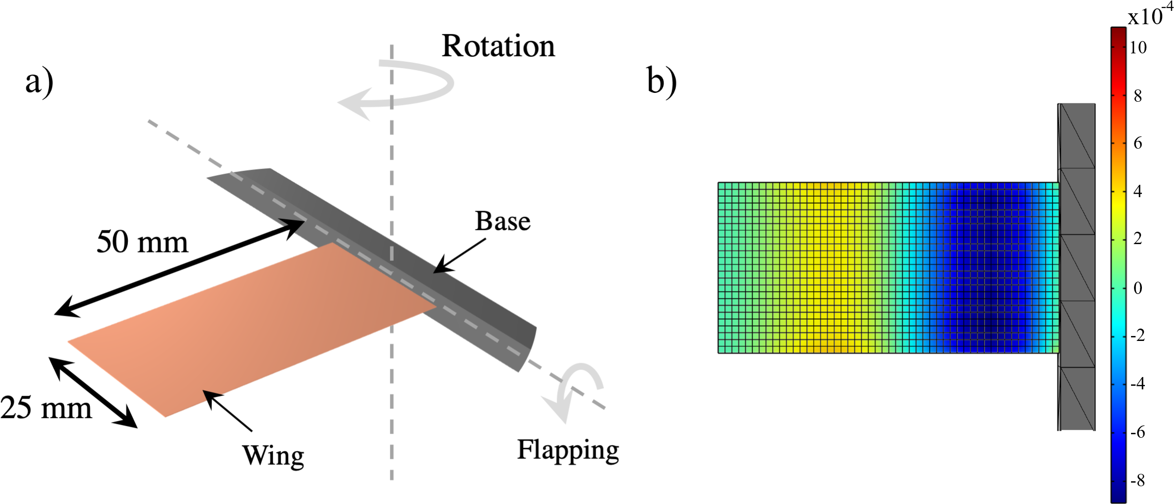
Figure 1: (a) Details of structural model and boundary conditions for flapping wing model in COMSOL, (b) meshing of the wing plate and normal strain distribution on the top surface of wing.

The random function in COMSOL software allowed us to use a random seed that is guaranteed to generate a new noise sequence while maintaining the same distribution. Proportionally to the nominal trajectory, we picked $Q=\mathrm{diag}{(1,1\times 10^{-4})}($\text{\,}\mathrm{rad}\text{\,}{\mathrm{s}}^{-1}$)^{2}$ where the larger variance corresponds to the noise on the flapping rate.

Table 1: Material Properties Used in COMSOL Simulations

Properties	Values
Young’s Modulus ($E$)	$0.3\text{\,}\mathrm{GPa}$
Poisson’s Ratio	0.35
Mass Damping Coefficient ($\alpha$)	$500\text{\,}{\mathrm{s}}^{-1}$
Stiffness Damping Coefficient ($\beta$)	$0\text{\,}\mathrm{s}$
Density	$1180\text{\,}\mathrm{k}\mathrm{g}\mathrm{/}\mathrm{m}^{3}$

For each simulation, we extracted the normal strain along the length of the wing (Fig. 1b) to feed into the neural encoding model, which is outlined in the following subsection.

4.2 Neural Encoding Measurement Model

We used a neural encoding model Pratt et al. [2017] to obtain the probability of firing of a neuron from the strain information at the location of the corresponding sensor. The model consists of a linear filter and a nonlinear activation function, NLA. The filter coefficients are determined using the spike-triggered average (STA),

$$\operatorname{STA}(t)=\cos{\left(2\pi f_{\text{STA}}(-t+a)\right)}\operatorname{exp}{\left(\frac{-(-t+a)^{2}}{b^{2}}\right)}.$$ (12)

Here, $b$, $f_{\text{STA}}$, and $a$ are the width, the STA frequency, and the delay, respectively. The similarity metric for a new stimulus, $\epsilon$, with the STA is obtained by convolving them and scaling by a constant, $C_{\xi}$:

$$\xi(x,y,t)=\frac{1}{C_{\xi}}\int_{0}^{N}\epsilon(x,y,t-\tau)\cdot STA(\tau)d\tau.$$ (13)

The NLA function determines the probability of firing, $P_{\text{fire}}$, based the projected stimulus, $\xi$:

$$P_{\text{fire}}=NLA(\xi)=\frac{1}{1+\exp(-c(\xi-d))}.$$ (14)

Here, $c$ is the slope and $d$ is the half-maximum position of the $\operatorname{NLA}$ function; the $x$, $y$ and $t$ arguments have been dropped for brevity. Notice that $P_{\text{fire}}$ at a time $t$ is not only a function of the strain value at that time but also includes an output delay with a length $N$.

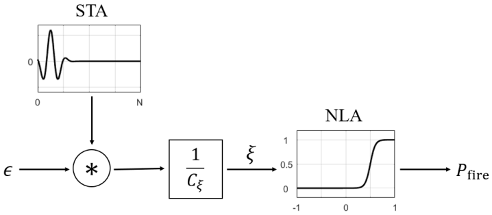
Figure 2: The probabilistic firing model of a neuron where the input is the strain information, $\epsilon$, and the output is the probability of firing, $P_{\text{fire}}$ Boyacıoğlu and Morgansen [2021].

The full neural encoding process is summarized in Fig. 2. In our application, the input to the neural encoding model is the strain at a location on the wing, and the output is $P_{\text{fire}}$. The encoder is experimentally validated in Pratt et al. [2017], and the parameters are regarded as constant for the neuron’s model. By considering $P_{\text{fire}}$ as the output of the system, we keep the neural encoding model deterministic. This way, the only source of uncertainty will be the process noise.

5 SENSOR PLACEMENT METHODOLOGY

Based on the output energy from different sensor locations of a system, one could expect different levels of observability. In this section, we present a sensor placement methodology based on the spectrum of the stochastic observability Gramian. To obtain the information of interest, we perform Monte Carlo analysis where the number of simulations was chosen based on convergence of the results.

Let $j:\mathbb{R}^{n\times n}\to\mathbb{R}$ be an unobservability metric as a function of the observability Gramian. Then the mean value of this metric obtained from $K$ simulations,

$$\hat{J}(t_{1},\mathbf{x}_{0},\mathbf{u})=\frac{1}{K}\sum_{i=1}^{K}j((W_{o}^{\varepsilon})_{i}),$$ (15)

should be minimized for the sensor placement problem. In other words, if $p$ is the finite number of possible sensor locations and we define ${(W_{o}^{\varepsilon})_{k}}_{i}$ as the Gramian matrix obtained at the $k$-th sensor location on the $i$-th run, then

$$(W_{o}^{\varepsilon})_{i}(\mathbf{\gamma})=\sum_{k=1}^{p}\gamma_{k}{(W_{o}^{\varepsilon})_{k}}_{i},$$ (16)

where $\gamma$ is the vector of Boolean-valued sensor activation functions, $\gamma_{i}$. The optimal sensor selection problem can be formulated as

$$\min\limits_{\gamma} \hat{J}(\gamma)$$ (17)

subject to $$\sum\gamma=r$$

$$\gamma_{k}\in\{0,1\},$$

where $r\leq p$ is the desired number of sensors. We are currently unaware of a convex relaxation for $j$ if it is the condition number or the unobservability index when $K>1$.

To deal with the non-convexity of (17), we applied the particle swarm optimization (PSO) algorithm, a metaheuristic approach introduced in Kennedy and Eberhart [1995]. The PSO algorithm is a technique that generates several solution candidates, i.e., particles, and updates their position and velocity according to certain rules until a termination criterion is met Kennedy and Eberhart [1995]. Since this method is not problem-specific and allows abstract level description Blum and Roli [2003], it is straightforward to implement. It also permits the definition of a search region, which is not the case for some widely-used algorithms such as the downhill simplex method Nelder and Mead [1965].

The pure PSO does not guarantee identification of the absolute local minimum. Hence, its hybridization with other optimization algorithms has been studied to find a better solution Thangaraj et al. [2011]. We also followed a hybrid approach, and at the expense of some computation time, used the result from PSO to initiate a second search by the interior point method (IPM) discussed in Byrd et al. [1999].

Note that the PSO algorithm requires a continuous search region, as opposed to be restricted to be able to have sensors at the $p$ potential locations in (14), and if each sensor has two coordinates to be determined, then the search space is $2r$-dimensional and the search would take more time as $r$ increases. To avoid having sensors too close to each other, we also implemented a relatively large positive value, $\sigma$, as the penalty for proximity.

The following pseudocode summarizes our approach to optimal sensor placement in a continuous space with upper and lower bounds, $ub$ and $lb$. Here, $d_{\min}$ is the minimum distance between any two of $r$ sensors, and $d_{\text{allowed}}$ is the minimum distance allowed. The PSO and IPM algorithm parameters have been suppressed for brevity.

Algorithm 1 Optimal Sensor Placement

1:procedure (dynamics, $ub$, $lb$, $j$, $K$, $r$, $d_{\text{allowed}}$, $\sigma$)

2:     define $(W_{o}^{\varepsilon})_{i}\leftarrow\sum_{k=1}^{r}{(W_{o}^{\varepsilon})_{k}}_{i}$

3:     define $\hat{J}\leftarrow\begin{cases}\frac{1}{K}\sum_{i=1}^{K}j((W_{o}^{\varepsilon})_{i})&d_{\min}\geq d_{\text{allowed}}\\ \sigma&d_{\min}<d_{\text{allowed}}\end{cases}$

4:     sensor loci $\leftarrow$ PSO($\hat{J}$,$ub$, $lb$)

5:     sensor loci $\leftarrow$ IPM($\hat{J}$,$ub$, $lb$, sensor loci)

6 NUMERICAL RESULTS

We now discuss the application results of the methods discussed here to the two example systems presented previously.

6.1 UAV Navigation System

As shown in prior work Hinson et al. [2013], a Lie algebraic approach for deterministic observability analysis can be used to show that the system (7) is unobservable if there is no control input, $\mathbf{u}(t)=\mathbf{0}$ and no noise, $\mathbf{w}=\mathbf{0}$. To explore the effects of noise, we simulated the control-free system with five different levels of process noise for $K=100$ simulations with $\mathbf{x}_{0}=\left[\begin{array}[]{lllll}0&0&\pi/6&0.35&-0.15\end{array}\right]^{\top}$ and $t_{1}=$150\text{\,}\mathrm{s}$$. Since the first two states are directly measured, we select the remaining states as states of interest. By allowing the nonzero process noise on $x_{1}$ and $x_{2}$, the stochastic empirical observability Gramian results in all nonsingular observability Gramians indicating an observable system.

Figure 3 shows the resultant unobservability metrics $\nu(W_{o}^{\epsilon})$ and $1/[\mathrm{det}(W_{o}^{\epsilon})]^{1/n}$. We observe a monotonic decrease in the unobservability index and its variance as the noise level increases. We also note the significant correlation between the two metrics, $\rho=0.87$, although this correlation depends on the system dynamics itself as well as $Q$.

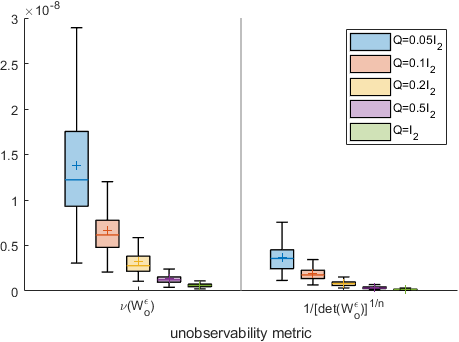
Figure 3: The change of two unobservability metrics as the noise level increases. Here, horizontal lines with color indicate the median value, and the plus sign denotes the mean. $I_{2}$ is the $2\times 2$ identity matrix.

If we define the unobservability metric as a linear combination of the condition number and the unobservability index,

$$j(W_{o}^{\epsilon})=\kappa(W_{o}^{\epsilon})+w_{\nu}\nu(W_{o}^{\epsilon}),$$ (18)

then the weight of $\nu(W_{o}^{\epsilon})$, $w_{\nu}$, will be of particular importance since $\kappa$ does not appear monotonic as a function of the noise, a characteristic which can be seen in Table 2 for $w_{\nu}=0$. Table 2 also illustrates this inference: as the unobservability index becomes dominant in the objective function, lower process noise on the system becomes less preferable.

Table 2: Observability Cost of UAV Navigation

	Process Noise Covariance, $Q$
$w_{\nu}$	$0.05I_{2}$	$0.1I_{2}$	$0.2I_{2}$	$0.5I_{2}$	$I_{2}$
$0$	$17.24$	$16.34$	$17.40$	$15.69$	$15.63$
$5\times 10^{8}$	$24.12$	$19.66$	$19.00$	$16.36$	$15.96$

6.2 Flapping Wing System

For this work, we studied optimal neural-inspired sensor placement on the system described in Sec. 4 aiming to increase observability. Particularly inspired/informed by a previous study Mohren et al. [2018] that showed that the existence of externally induced body rotation as large as $\omega=$10\text{\,}\mathrm{rad}\text{\,}{\mathrm{s}}^{-1}$$ on a flapping wing differs by a twisting mode three orders of magnitude smaller than the dominant flapping mode.

We simulated the FEA model for $0.2\text{\,}\mathrm{s}$ (5 wingbeats) using time step of $5\text{\times}{10}^{-4}\text{\,}\mathrm{s}$. The motion was prescribed through angular velocities of flapping and rotation. Both velocities were zero through the first wingbeat cycle and linearly increased to their maximum values ($\sim$$57\text{\,}\mathrm{rad}\text{\,}{\mathrm{s}}^{-1}$ for flapping and $0.02\text{\,}\mathrm{rad}\text{\,}{\mathrm{s}}^{-1}$ for rotation) over the course of the second cycle. We ran the simulation for two more cycles before introducing the perturbation, $\varepsilon=$0.01\text{\,}\mathrm{rad}\text{\,}{\mathrm{s}}^{-1}$$, to the system. As studied in Boyacıoğlu and Morgansen [2021], a regular cycle before the perturbation was necessary as the neural-encoded output has a delay, unlike the typical systems. The system was simulated one more cycle after the introduction of the perturbation, i.e., $t_{1}=$40\text{\,}\mathrm{ms}$$.

We took the neural encoding parameters to be $a=$5\text{\,}\mathrm{ms}$$, $b=$4\text{\,}\mathrm{ms}$$, $\omega_{\text{STA}}=$1000\text{\,}\mathrm{rad}\text{\,}{\mathrm{s}}^{-1}$$, $c=10$, $d=0.5$, and $N=$40\text{\,}\mathrm{ms}$$. The resultant distributions of the average unobservability index and the condition number stabilized in $K=40$ sets of simulations. In Fig. 4, it can be seen that the unobservability index increases almost monotonically from the wing root ($x=0$) to the wingtip ($x=-5$). On the other hand, there are two separate regions where the eigenvalues are relatively more balanced. Finally, note that the asymmetric distributions about the $x$-axis are caused by the nonzero rotation rate.

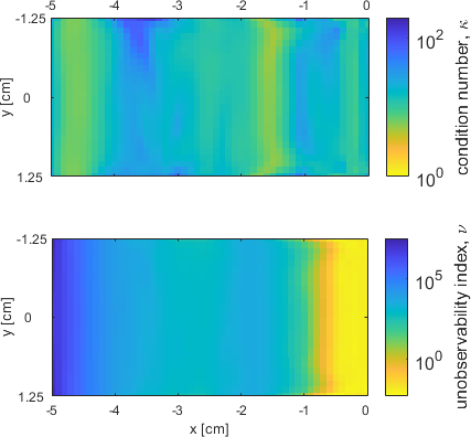
Figure 4: The average distribution of two unobservability metrics ($K=40$). Yellow regions are more observable than the dark blue ones.

We then ran the hybrid PSO algorithm for $r$ from one to $20$ to minimize the linear combination of $\kappa$ and $\nu$ with $w_{\nu}=0.1$ and to minimize solely the condition number, $w_{\nu}=0$. Since the search was performed in a continuous space, the strain value at a point was calculated as a weighted average of the strain values obtained for the neighboring FEA nodes. To avoid having sensors placed closer to each other than $1\text{\,}\mathrm{mm}$, we determined the penalty value as $\sigma=1\times 10^{5}$.

The observability cost for increasing numbers of desired sensors is given in Fig. 5 (top). Both the condition number and its linear combination with the unobservability index converge, and adding a new sensor does not improve the observability significantly, which might be partially caused by the increasing dimension of the search.

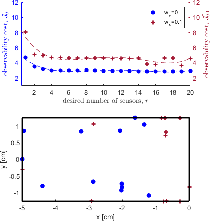
Figure 5: (top) The change of the observability costs by the number of sensors with fourth-degree polynomial fitting, (bottom) The optimal neural-inspired sensor placement for $r=12$. The figures use the same legend.

Lastly, the optimal sensor placement for $r=12$ is shown in Fig. 5 (bottom). When the linear combination of the two measures with $w_{\nu}=0.1$ was utilized instead of a single unobservability measure, the sensors were slightly shifted to the left, and at least one sensor was placed at each edge. The use of pure condition number ($w_{\nu}=0$) resulted in having no sensors in the regions where the output energy is highest.

7 CONCLUSIONS AND FUTURE WORK

We formulated an optimal sensor placement methodology based on the stochastic empirical Gramian and illustrated it for two systems with process noise. Since the problems are stochastic and non-convex, we performed Monte Carlo runs and used a metaheuristic optimization algorithm, PSO. We conclude that how the cost function is chosen matters, and a wise choice depends on the system structure and balances the output energy and the estimation condition.

In light of the results from the UAV example, we plan to continue investigating how better observability metrics result in better estimation performances. We will also study the convex relaxation of the optimization problem (17) for various stochastic observability Gramian-based objective functions in the future. Higher moments of the probabilistic distribution (variance, skewness, and so on) might also be considered while posing the optimization problem, e.g., trust levels for sensor location candidates can be determined by the variance of the unobservability metrics. Such an approach would be similar to the weighted least squares used in linear batch estimation Crassidis and Junkins [2011] or to the distributed least squares estimation in sensor networks Mesbahi and Egerstedt [2010].

A more realistic wing model can also be studied taking into account the actual wing profiles, nonuniform stiffness of the wing as in Weber et al. [2023], and the structure of the strain-sensitive biological sensors. Finally, the neural spikes can be considered as the system output instead of the probability of firing, $P_{\text{fire}}$, and the possible sensor locations can be constrained to be on the vein of an insect wing.

Key points to be addressed in the next steps of the work are direct assessment of the improvements in filter performance from the optimal sensor placement, exploration of the effects of different metrics on the filter performance, and impacts of neural decoding methodology as expressed in the system measurement functions.

Funding Sources

This work was funded in part by Air Force Office of Scientific Research (AFOSR) grants FA9550-19-1-0386 and FA9550-14-1-0398.

References

- Anguelova [2004] Milena Anguelova. Nonlinear Observability and Identifiability: General Theory and a Case Study of a Kinetic Model for S. cerevisiae. PhD thesis, Chalmers Univ. of Technology and Göteborg Univ., 2004.
- Blum and Roli [2003] Christian Blum and Andrea Roli. Metaheuristics in combinatorial optimization. ACM Computing Surveys, 35(3):268–308, 2003. doi:10.1145/937503.937505.
- Boyacıoğlu and Morgansen [2021] Burak Boyacıoğlu and Kristi A. Morgansen. Bioinspired observability analysis tools for deterministic systems with memory in flight applications. In AIAA SciTech Forum, 2021. doi:10.2514/6.2021-1679.
- Byrd et al. [1999] Richard H. Byrd, Mary E. Hribar, and Jorge Nocedal. An interior-point algorithm for large-scale nonlinear programming. SIAM Journal on Optimization, 9(4):877–900, 1999. doi:10.1137/S1052623497325107.
- Combes and Daniel [2003] S. A. Combes and T. L. Daniel. Flexural stiffness in insect wings I. Scaling and the influence of wing venation. Journal of Experimental Biology, 206(17):2979–2987, 2003. doi:10.1242/jeb.00523.
- Crassidis and Junkins [2011] John L. Crassidis and John L. Junkins. Optimal Estimation of Dynamic Systems. Chapman & Hall/CRC, 2nd edition, 2011.
- Dochain et al. [1997] D. Dochain, N. Tali-Maamar, and J. P. Babary. On modelling, monitoring and control of fixed bed bioreactors. Computers & Chemical Engineering, 21(11):1255–1266, 1997. ISSN 0098-1354. doi:10.1016/S0098-1354(96)00370-5.
- Dragan and Morozan [2004] Vasile Dragan and Toader Morozan. Stochastic observability and applications. IMA Journal of Mathematical Control and Information, 21(3):323–344, 2004. doi:10.1093/imamci/21.3.323.
- Eberle et al. [2015] A. L. Eberle, B. H. Dickerson, P. G. Reinhall, and T. L. Daniel. A new twist on gyroscopic sensing: Body rotations lead to torsion in flapping, flexing insect wings. Journal of The Royal Society Interface, 12(104):20141088, 2015. doi:10.1098/rsif.2014.1088.
- Glotzbach et al. [2014] Thomas Glotzbach, Naveena Crasta, and Christoph Ament. Observability analyses and trajectory planning for tracking of an underwater robot using empirical gramians. IFAC Proc. Volumes, 47(3):4215–4221, 2014. doi:10.3182/20140824-6-ZA-1003.01939.
- Himpe [2018] Christian Himpe. emgr—the empirical Gramian framework. Algorithms, 11(7):91, 2018. doi:10.3390/a11070091.
- Hinson and Morgansen [2015] Brian T. Hinson and Kristi A. Morgansen. Gyroscopic sensing in the wings of the hawkmoth Manduca sexta: The role of sensor location and directional sensitivity. Bioinspiration & Biomimetics, 10(5):056013, 2015. doi:10.1088/1748-3190/10/5/056013.
- Hinson et al. [2013] Brian T. Hinson, Michael K. Binder, and Kristi A. Morgansen. Path planning to optimize observability in a planar uniform flow field. In Proc. American Control Conf., pages 1392–1399, 2013. doi:10.1109/ACC.2013.6580031.
- Kennedy and Eberhart [1995] James Kennedy and Russell Eberhart. Particle swarm optimization. In Proc. Int. Conf. on Neural Networks, pages 1942–1948, 1995. doi:10.1109/ICNN.1995.488968.
- Krener and Ide [2009] Arthur J. Krener and Kayo Ide. Measures of unobservability. In Proc. of the 48h IEEE Conf. on Decision and Control held jointly with 28th Chinese Control Conf., pages 6401–6406, 2009. doi:10.1109/CDC.2009.5400067.
- Lall et al. [1999] Sanjay Lall, Jerrold E. Marsden, and Sonja Glavaški. Empirical model reduction of controlled nonlinear systems. IFAC Proc. Volumes, 32(2):2598–2603, 1999. doi:10.1016/S1474-6670(17)56442-3.
- Mesbahi and Egerstedt [2010] Mehran Mesbahi and Magnus Egerstedt. Graph Theoretic Methods in Multiagent Networks. Princeton University Press, 2010.
- Mohren et al. [2018] Thomas L. Mohren, Thomas L. Daniel, Steven L. Brunton, and Bingni W. Brunton. Neural-inspired sensors enable sparse, efficient classification of spatiotemporal data. Proc. of the National Academy of Sciences, 115(42):10564–10569, 2018. doi:10.1073/pnas.1808909115.
- Müller and Weber [1972] P. C. Müller and H. I. Weber. Analysis and optimization of certain qualities of controllability and observability for linear dynamical systems. Automatica, 8(3):237–246, 1972. doi:10.1016/0005-1098(72)90044-1.
- Nelder and Mead [1965] J. A. Nelder and R. Mead. A simplex method for function minimization. The Computer Journal, 7(4):308–313, 1965. doi:10.1093/comjnl/7.4.308.
- Powel and Morgansen [2020] Nathan Powel and Kristi A. Morgansen. Empirical observability Gramian for stochastic observability of nonlinear systems. arXiv e-prints, 2020. doi:10.48550/arXiv.2006.07451.
- Powel and Morgansen [2015] Nathan D. Powel and Kristi A. Morgansen. Empirical observability Gramian rank condition for weak observability of nonlinear systems with control. In Proc. of the 54th IEEE Conf. on Decision and Control, pages 6342–6348, 2015. doi:10.1109/CDC.2015.7403218.
- Pratt et al. [2017] Brandon Pratt, Tanvi Deora, Thomas Mohren, and Thomas Daniel. Neural evidence supports a dual sensory-motor role for insect wings. Proc. of the Royal Society B: Biological Sciences, 284(1862):20170969, 2017. doi:10.1098/rspb.2017.0969.
- Qi et al. [2015] Junjian Qi, Kai Sun, and Wei Kang. Optimal PMU placement for power system dynamic state estimation by using empirical observability Gramian. IEEE Trans. on Power Systems, 30(4):2041–2054, 2015. doi:10.1109/TPWRS.2014.2356797.
- Serpas et al. [2013] Mitch Serpas, Gabriel Hackebeil, Carl Laird, and Juergen Hahn. Sensor location for nonlinear dynamic systems via observability analysis and max-det optimization. Computers & Chemical Engineering, 48:105–112, 2013. doi:10.1016/j.compchemeng.2012.07.014.
- Singh and Hahn [2005] Abhay K. Singh and Juergen Hahn. Determining optimal sensor locations for state and parameter estimation for stable nonlinear systems. Industrial & Engineering Chemistry Research, 44(15):5645–5659, 2005. doi:10.1021/ie040212v.
- Sontag [1998] Eduardo D. Sontag. Mathematical Control Theory: Deterministic Finite Dimensional Systems. Springer-Verlag, 1st edition, 1998.
- Thangaraj et al. [2011] Radha Thangaraj, Millie Pant, Ajith Abraham, and Pascal Bouvry. Particle swarm optimization: Hybridization perspectives and experimental illustrations. Applied Mathematics and Computation, 217(12):5208–5226, 2011. doi:10.1016/j.amc.2010.12.053.
- Weber et al. [2023] Alison I. Weber, Mahnoush Babaei, Amanuel Mamo, Bingni W. Brunton, Thomas L. Daniel, and Sarah Bergbreiter. Nonuniform structural properties of wings confer sensing advantages. Journal of the Royal Society Interface, 20(200):20220765, 2023. doi:10.1098/rsif.2022.0765.