HyperMask: Adaptive Hypernetwork-based Masks for Continual Learning

Abstract

Artificial neural networks suffer from catastrophic forgetting when they are sequentially trained on multiple tasks. Many continual learning (CL) strategies are trying to overcome this problem. One of the most effective is the hypernetwork-based approach. The hypernetwork generates the weights of a target model based on the task’s identity. The model’s main limitation is that, in practice, the hypernetwork can produce completely different architectures for subsequent tasks. To solve such a problem, we use the lottery ticket hypothesis, which postulates the existence of sparse subnetworks, named winning tickets, that preserve the performance of a whole network. In the paper, we propose a method called HyperMask, which trains a single network for all CL tasks. The hypernetwork produces semi-binary masks to obtain target subnetworks dedicated to consecutive tasks. Moreover, due to the lottery ticket hypothesis, we can use a single network with weighted subnets. Depending on the task, the importance of some weights may be dynamically enhanced while others may be weakened. HyperMask achieves competitive results in several CL datasets and, in some scenarios, goes beyond the state-of-the-art scores, both with derived and unknown task identities.

1 Introduction

Figure 1: Commonly, the parameters of a neural network are directly adjusted from data to solve a task. In HyperMask hypernetwork maps embedding vectors $e_{i}$ to the semi-binary mask, producing a subnetwork dedicated to the target network to solve the $i$–th task. Finally, a subset of weights was switched off (removed connections in the right-side image) while the remaining weights were scored continuously from 0 to 1 (weights of different thicknesses).

Learning from a continuous data stream is challenging for deep learning models. Artificial neural networks suffer from catastrophic forgetting (McCloskey and Cohen, 1989) and drastically forget previously known information upon learning new knowledge. Continual learning (CL) Hsu et al. (2018) methods aim to learn consecutive tasks and prevent forgetting already learned ones effectively.

One of the most promising approaches to CL is the hypernetwork von Oswald et al. (2019); Henning et al. (2021) approach. A hypernetwork architecture Ha et al. (2016) is a neural network that generates weights for a separate target network designated to solve a specific task. In a continual learning setting, a hypernetwork generates the weights of a target model based on the task identity. At the end of training, we have a single meta-model, which produces dedicated weights. Due to the ability to generate completely different weights for each task, hypernetwork-based models feature minimal forgetting. Unfortunately, such properties were obtained by producing completely different architectures for substantial tasks. Only hypernetworks use information about tasks. Such a model can produce different nets for each task and solve them separately. The hypernetwork cannot use the weight of the target network from the previous task.

To solve such a problem, we use the lottery ticket hypothesis (LTH) Frankle and Carbin (2018), which postulates that we can find subnetworks named winning tickets with performance similar (or even better) to the full architecture. However, the search for optimal winning tickets in continual learning scenarios is difficult Mallya et al. (2018); Wortsman et al. (2020), as consecutive learning steps require repetitive pruning and retraining for each arriving task, which is impractical. Alternatively, Winning SubNetworks (WSN) Kang et al. (2022) incrementally learns model weights and task-adaptive binary masks. WSN eliminates catastrophic forgetting by freezing the subnetwork weights considered essential for the previous tasks and memorizing masks for all tasks.

Our paper proposes a method called HyperMask which combines hypernetwork and lottery ticket hypothesis paradigms. Hypernetwork produces semi-binary masks to the target network to obtain weighted subnetworks dedicated to new tasks; see Fig. 1. By semi-binary masks, we mean that some weights may be turned off for selected tasks while the remaining weights are scored between 0 and 1. The masks produced by the hypernetwork modulate the weights of the main network and act like dynamic filters, enhancing the important target weights for a given task and decreasing the importance of the remaining weights. Additionally, a subset of weights may be excluded from contribution in a given task by sparsifying the mask. Consequently, we work on a single network with subnetworks dedicated to each task and do not need to freeze any part of this model. When HyperMask learns a new task, we reuse the learned subnetwork weights from the previous tasks. HyperMask also inherits the ability of the hypernetwork to adapt to new tasks with minimal forgetting. We produce a semi-binary mask directly from the trained task embedding vector, which creates a dedicated subnetwork for each dataset.

To the best of our knowledge, our model is the first architecture-based CL model that uses hypernetwork, or, in general, any meta-model, for producing masks for other networks. Updates of hypernetworks are prepared not directly for the weights of the main model, like in von Oswald et al. (2019), but for masks dynamically filtering the target model.

Our contributions can be summarized as follows:

• We propose a method that uses the hypernetwork paradigms for modelling the lottery ticket-based subnetwork. The hypernetwork modulates the weights of the main model instead of their direct preparation as in von Oswald et al. (2019).

• We show that HyperMask is able to reuse weights from the lottery ticket module and adapt to new tasks from the hypernetwork paradigm.

• We demonstrate that HyperMask achieves competitive results for the presented CL datasets and obtains state-of-the-art scores for some demanding scenarios, both with known and unknown task identities.

2 Related Works

Continual learning

Typically, continual learning approaches are divided into three main categories: regularization, dynamic architectures, and replay-based techniques (Parisi et al., 2019; De Lange et al., 2021; Wang et al., 2023). HyperMask model represents dynamic architectures.

Architecture-based approaches use dynamic architectures which dedicate separate model branches to different tasks. These branches can be developed incrementally, such as in the case of Progressive Neural Networks Rusu et al. (2016). The architecture of such a system can be optimized to enhance parameter effectiveness and knowledge transfer, for example, by reinforcement learning (RCL (Xu and Zhu, 2018), BNS (Qin et al., 2021)), architecture search (LtG (Li et al., 2019), BNS (Qin et al., 2021)), and variational Bayesian methods (BSA (Kumar et al., 2021)). Alternatively, a static architecture can be reused with iterative pruning as proposed by PackNet (Mallya and Lazebnik, 2018) or by applying Supermasks (Wortsman et al., 2020).

In PackNet Mallya and Lazebnik (2018), during the training of consecutive tasks, a subset of available network weights is selected while the rest is pruned. Furthermore, weights considered important for some tasks must remain unchanged and cannot be pruned in the future. Therefore, the space for modifying weights is getting smaller along with subsequent tasks. In HyperMask, we can create any number of embeddings and different semi-binary masks so that the target network weights can be filtered dynamically. These weights are also continuously scored and do not have to be switched on or off, like in PackNet.

Recent works are focused on efficiently using of a feature extractor fixed after the first learning stage. FeTrIL Petit et al. (2023) proposes a new approach which combines a fixed feature extractor and a pseudo-features generator. The generator uses geometric translations to produce a favourable representation of old classes based on new classes. In FeCAM Goswami et al. (2023), a fixed feature extractor is used to build representations of elements in each class separately. Then, the class prototype and a corresponding covariance matrix are estimated. The final predictions are obtained by the calculation of the Mahalanobis distance between samples and different class representations. Both methods work in class incremental settings.

Pruning-based Continual Learning

Most architecture-based methods use additional memory to obtain better performance. In the pruning-based method, we build computationally- and memory-efficient strategies.

CLNP (Golkar et al., 2019) freezes the most significant parts of the network and divides it into active, inactive and interference parts. This pruning approach is based on neuron average activity. Therefore, the model maintained its performance after learning of the following tasks. However, the current model’s performance and capacity for the upgoing tasks must be compromised.

Piggyback (Mallya et al., 2018) uses a pre-trained model and task-specific binary masks. In contrast, HyperMask for all the target network weights considered important, create their continuous score between 0 and 1. Also, in PiggyBack, the base network weights are frozen while HyperMask simultaneously trains the hyper- and the target network.

HAT (Serra et al., 2018) uses task-specific learnable attention vectors to recognize significant weights for each task and dynamically creates or destroys paths between single network units. Furthermore, a cumulative attention vector is created. In HyperMask, masks are produced by a meta-model and depend on the trained embedding vectors.

LL-Tickets (Chen et al., 2020) show that we can find a subnetwork, referred to as lifelong tickets, which performs well on all tasks during continual learning. If the tickets cannot work on the new task, the method looks for more prominent tickets from the existing ones. However, the LL-Tickets expansion process is made up of a series of retraining and pruning steps.

In Winning SubNetworks (WSN) Kang et al. (2022), authors propose to jointly learn the model and task-adaptive binary masks dedicated to task-specific subnetworks (winning tickets). Unfortunately, WSN eliminates catastrophic forgetting by freezing the subnetwork weights for the previous tasks and memorizing masks for all tasks. Meanwhile, HyperMask dynamically enhances important target weights for a given task and decreases the significance of the remaining weights.

This paper proposes the next step toward producing a sparse subnetwork for continual learning. Instead of the classical binary mask and freezing strategy, we use the hypernetwork paradigm.

Hypernetworks for continual learning

A hypernetwork Ha et al. (2016) is an architecture which generates a vector of weights for a separate target network designated to solve a specific task. Hypernetworks are widely used, e.g. in generative models Spurek et al. (2020), building implicit representation Szatkowski et al. (2023) and few-shot learning Sendera et al. (2023).

In a continuous learning environment, a hypernetwork generates the weights of a target model based on the task’s identity. HNET von Oswald et al. (2019) uses task embeddings to produce weights dedicated to each task. HNET can be seen as an architecture-based strategy as we create a distinct architecture for each task. However, it can also be viewed as a regularization model. After training, a single meta-model that produces specialized weights is left. Hypernetworks can generate different nets for tasks and, in some sense, solve them independently. While in HNET, a meta-model generates target network weights directly, in HyperMask, a meta-model prepares masks for the target network adapted for consecutive tasks.

In Henning et al. (2021), authors propose a Bayesian version of the hypernetworks in which they produce parameters of the prior distribution of the Bayesian network.

3 HyperMask: Adaptive Hypernetworks for Continual Learning

Our proposition, called HyperMask, is a hypernetwork-based continual learning method. In HyperMask, the hypernetwork returns semi-binary masks to produce weighted target subnetworks dedicated to new tasks. This solution inherits the ability of the hypernetwork to adapt to new tasks with minimal forgetting and uses the lottery ticket hypothesis to create a single network with weighted masks.

Problem statement

Let us consider a supervised learning setup where $T$ tasks are derived to a learner sequentially. We assume that $X_{t}=\{\bm{x}_{i,t}\}^{n_{t}}_{i=1}$ is the dataset for task $t$, composed of $n_{t}$ elements of raw instances and $Y_{t}=\{y_{i,t}\}^{n_{t}}_{i=1}$ are the corresponding labels, $t\in\{1,2,...,T\}$. Data from task $t$ we denote by $D_{t}=(X_{t},Y_{t})~{}\subset~{}X~{}\times~{}Y$. We assume a neural network $f(\cdot;\bm{\theta})$, parameterized by the model weights $\bm{\theta}$ and the standard continual learning scenario

$$\bm{\theta}^{*}=\operatorname*{arg\,min}\limits_{\bm{\theta}}\frac{1}{n_{t}}\sum_{i=1}^{n_{t}}\mathcal{L}\big{(}f(\bm{x_{i,t}};\bm{\theta})\big{)},$$

where $\mathcal{L}(\cdot,\cdot)$ is a classification objective loss such as the cross-entropy loss. We assume that $D_{t}$ for task $t$ is only accessible when learning task $t$. Also, the task identity is given in both the training and testing stages, except for the additional series of experiments described further.

To provide space for learning future tasks, a continuing learner often adopts over-parameterized deep neural networks. In such situations, we can find subnets with equal or better performance.

Hypernetwork

Hypernetworks, introduced in Ha et al. (2016), are defined as neural models that generate weights for a separate target network solving a specific task. Before we present our solution, we describe the classical approach to using hypernetworks in CL. A hypernetwork generates individual weights for all tasks in a continual learning setting. In HNET von Oswald et al. (2019); Henning et al. (2021) the authors propose using trainable embeddings $\bm{e}_{t}\in\mathbb{R}^{N}$, where $t\in\{1,...,T\}$. The hypernetwork $\mathcal{H}$ with weights $\bm{\Phi}$ generates weights $\bm{\theta}_{t}$ of the target network $f$ dedicated to the $t$–th task

$$\mathcal{H}(\bm{e}_{t};\bm{\Phi})=\bm{\theta}_{t}.$$

HNET meta-architecture (hypernetwork) produces different weights for each continual learning task. We have the function $f_{\bm{\theta}_{t}}:X\to Y$ (a neural network classifier with weights $\bm{\theta}_{t}$), which predicts labels based on data samples from a continuous learning dataset.

The target network is not trained directly. In HNET, we use a hypernetwork $H_{\bm{\Phi}}:\mathbb{R}^{N}\ni\bm{e}_{t}\to\bm{\theta}_{t}$, which for a task embedding $\bm{e}_{t}$ returns weights $\bm{\theta}_{t}$ of the corresponding target network $f_{\bm{\theta}_{t}}:X\to Y$. Thus, each continual learning task is represented by a function (classifier)

$$f_{\bm{\theta}_{t}}=f(\cdot;\bm{\theta}_{t})=f\big{(}\cdot;H(\bm{e}_{t};\bm{\Phi})\big{)}.$$

At the end of training, we have a single meta-model, which produces dedicated weights. Due to the ability to generate completely different weights for each task, hypernetwork-based models feature minimal forgetting. We practically produce a new architecture when we update the prior task. To solve such a problem, in HyperMask, we use the lottery ticket hypothesis, which postulates the existence of sparse subnetworks, named winning tickets, that preserve the performance of a whole network.

Algorithm 1 The pseudocode of HyperMask.

hypernetwork $\mathcal{H}$ with weights $\bm{\Phi}$, target network $f$ with weights $\bm{\theta}$, sparsity $p\geq 0$, regularization strength $\beta>0$, and $\lambda>0$, $n$ training iterations, datasets $\{D_{1},D_{2},...,D_{T}\}$, $(\bm{x}_{i,t},y_{i,t})\in D_{t},t\in\{1,...,T\}$

updated hypernetwork weights $\bm{\Phi}$, updated target network weights $\bm{\theta}$

Initialize randomly weights $\bm{\Phi}$ and $\bm{\theta}$ with embeddings $\{\bm{e}_{1},\bm{e}_{2},...,\bm{e}_{T}\}$

for $t\leftarrow 1$ to $T$ do

     if $t>1$ then

         $\bm{\theta}^{*}\leftarrow\bm{\theta}$

         for $t^{\prime}\leftarrow 1$ to $t-1$ do

              Store $\bm{m}_{t^{\prime}}\leftarrow\mathcal{H}(\bm{e}_{t^{\prime}},p;\bm{\Phi})$

         end for

     end if

     for $i\leftarrow 1$ to $n$ do

         $\bm{m}_{t}\leftarrow\mathcal{H}(\bm{e}_{t},p;\bm{\Phi})$

         $\bm{\theta}_{t}\leftarrow\bm{m}_{t}\odot\bm{\theta}$

         $\hat{y}_{i,t}\leftarrow f(\bm{x}_{i,t};\bm{\theta}_{t})$

         if $t=1$ then

              $\mathcal{L}\leftarrow\mathcal{L}_{current}$ 

         else

              $\mathcal{L}\leftarrow\mathcal{L}_{current}+\beta\cdot\mathcal{L}_{output}+\lambda\cdot\mathcal{L}_{target}$ 

         end if

         Update $\bm{\Phi}$ and $\bm{\theta}$

     end for

     Store $\bm{e}_{t}$

end for

3.1 HyperMask – overview

In HyperMask, a hypernetwork $\mathcal{H}_{\bm{\Phi}}:\mathbb{R}^{N}\ni\mathbf{e}_{t}\to\bm{m}_{t},$ where $t\in\{1,...,T\}$, produces semi-binary masks which are multiplied element-wise with the target network weights. Similarly, as in HNET, we use trainable embeddings $\bm{e}_{t}$ to prepare masks adapted to a given task.

Mask creation

To ensure that a mask has a continuous representation ranging from 0 to 1, we use the tanh activation function on the hypernetwork output. Then, we select the $p\%$ weights with the highest weight scores, where $p$ is the ratio of the target layer capacity and $c(p,i,t;\mathbf{x})$ is a threshold value for the selected target layer $\mathbf{x}$, during the $i$-th training iteration of the $t$-th task. The choice of weights is performed through the task-dependent semi-binary weight mask $\bm{m}_{t}$, where an absolute value greater than the threshold denotes that the weight is taken into account during the forward pass and is zeroed otherwise. Formally, $\bm{m}_{t}$ is obtained by applying an indicator function $\sigma_{p}(\cdot;\cdot)$ to a weight $w$ that is an element of $\mathbf{x}$ representing a single layer of the output of $\mathcal{H}$

$$\sigma_{p}(w;\mathbf{x})=\left\{\begin{array}[]{@{}ll@{}}0&\text{if}\ |w|\leq c(p,i,t;\mathbf{x}),\\ w&\text{otherwise}.\end{array}\right.$$

Additionally, the ratio $p$ is constant starting from the second task but, for the first trained task, is gradually increased from $0$ to $p$

$$c(p,i,t;\mathbf{x})=\left\{\begin{array}[]{@{}ll@{}}P(p;|\mathbf{x}|)&\text{if}\ t>1,\\ P(\frac{i}{n}\cdot p;|\mathbf{x}|)&\text{otherwise}.\end{array}\right.$$

$P(p;|\mathbf{x}|)$ represents the $p$-th percentile of the set of absolute values of a given mask layer. Each task is trained through $n$ iterations. The absolute value of consecutive $\mathbf{x}$ weights is calculated element-wise.

Therefore, HyperMask uses trainable embeddings $\mathbf{e}_{t}\in\mathbb{R}^{N}$ for $t\in\{1,...,T\}$, threshold level $p$ and hypernetwork $\mathcal{H}$ with weights $\bm{\Phi}$ generating a semi-binary mask $\bm{m}_{t}$ (with $p\%$ zeros) adapted to each task and applied for the target network weights $\bm{\theta}$

$$\mathcal{H}(\mathbf{e}_{t},p;\bm{\Phi})=\sigma_{p}\big{(}:,\mathcal{H}(\mathbf{e}_{t};\bm{\Phi})\big{)}=\bm{m}_{t};$$

$\sigma_{p}(:,\cdot)$ means that the indicator function is applied for all output values of $\mathcal{H}$.

Target network

In HyperMask, we have two trainable architectures. In addition to $\mathcal{H}$, the target network $f$ has its trainable parameters $\bm{\theta}$. More precisely, we model the function $f_{\bm{\theta}}:X\to Y$ with general weights $\bm{\theta}$ designed for all tasks. The hypernetwork $\mathcal{H}$ and the target network $f$ are simultaneously trained with a cross-entropy loss function. Thus, each continual learning task is represented by a function (classifier)

$$f(\cdot;\bm{\theta}\odot\bm{m}_{t})=f\big{(}\cdot;\bm{\theta}\odot\mathcal{H}(\mathbf{e}_{t},p;\bm{\Phi})\big{)},$$

where $\odot$ is element-wise multiplication.

In the training procedure, we have added two regularization terms. The first one is the output regularizer proposed by Li and Hoiem (2017):

$$\mathcal{L}_{output}=\sum_{t=1}^{T-1}\sum_{i=1}^{|X_{t}|}\|f(\mathbf{x}_{i,t};\bm{\theta}^{*}\odot\bm{m}_{t})-f(\mathbf{x}_{i,t};\bm{\theta}\odot\bm{m}_{t})\|^{2},$$

where $\bm{\theta}^{*}$ is the set of the target network parameters before attempting to learn task $T$.

This solution is expensive in terms of memory and does not follow the online learning paradigm adequately. However, hypernetworks von Oswald et al. (2019); Henning et al. (2021) avoid this problem. Task-conditioned hypernetworks produce an output depending on the task embedding. We can compare the fixed hypernetwork output produced before learning task $T$ with weights $\bm{\Phi}^{*}$, with the output after a current proposition of hypernetwork weight modifications $\Delta\bm{\Phi}$, according to the cross-entropy loss. Finally, in HyperMask, the output regularization loss is given by:

$$\mathcal{L}_{output}(\bm{\Phi}^{*},\bm{\Phi},\Delta\bm{\Phi},\{\mathbf{e}_{t}\})$$

$$= \frac{1}{T-1}\sum_{t=1}^{T-1}\|\mathcal{H}(\mathbf{e}_{t},0;\bm{\Phi}^{*})-\mathcal{H}(\mathbf{e}_{t},0;\bm{\Phi}+\Delta\bm{\Phi})\|^{2},$$

where $\Delta\bm{\Phi}$ is considered fixed. We do not sparse the hypernetwork weights at this stage therefore $p=0$.

The difference between HyperMask and von Oswald et al. (2019) relies on the fact that using $\mathcal{L}_{output}$, we just regularize masks dedicated to consecutive continual learning tasks and not the target weights.

Table 1: Mean overall accuracy with a standard deviation of different continual learning methods. We obtained better results than our primary baselines: WSN and HNET. Moreover, we have the best results on CIFAR-100 and Tiny ImageNet. Details about experimental scenarios and HyperMask hyperparameters are presented in Appendix B. Results for different methods than HyperMask are derived from other papers. ^∗ denotes a model trained on ResNet-20, ^∗∗ on ZenkeNet while ^⊛ on the reduced ZenkeNet architecture.

Method	Permuted MNIST	Split MNIST	Split CIFAR-100	Tiny ImageNetHAT	$\mathbf{97.67\pm 0.02}$	$-$	$72.06\pm 0.50$	$-$
GPM	$94.96\pm 0.07$	$-$	$73.18\pm 0.52$	$67.39\pm 0.47$
PackNet	$96.37\pm 0.04$	$-$	$72.39\pm 0.37$	$55.46\pm 1.22$
SupSup	$96.31\pm 0.09$	$-$	$75.47\pm 0.30$	$59.60\pm 1.05$
La-MaML	$-$	$-$	$71.37\pm 0.67$	$66.99\pm 1.65$
FS-DGPM	$-$	$-$	$74.33\pm 0.31$	$70.41\pm 1.30$WSN, $c=3\%$	$94.84\pm 0.11$	$-$	$70.65\pm 0.36$	$68.72\pm 1.63$
WSN, $c=5\%$	$95.65\pm 0.03$	$-$	$72.44\pm 0.27$	$71.22\pm 0.94$
WSN, $c=10\%$	$96.14\pm 0.03$	$-$	$74.55\pm 0.47$	$71.96\pm 1.41$
WSN, $c=30\%$	$96.41\pm 0.07$	$-$	$75.98\pm 0.68$	$70.92\pm 1.37$
WSN, $c=50\%$	$96.24\pm 0.11$	$-$	$76.38\pm 0.34$	$69.06\pm 0.82$
WSN, $c=70\%$	$96.29\pm 0.00$	$-$	$-$	$-$EWC	$95.96\pm 0.06$	$99.12\pm 0.11$	$72.77\pm 0.45$	$-$
SI	$94.75\pm 0.14$	$99.09\pm 0.15$	$-$	$-$
DGR	$97.51\pm 0.01$	$99.61\pm 0.02$	$-$	$-$
HNET+ENT	$97.57\pm 0.02$	$\mathbf{99.79\pm 0.01}$	$-$	$-$ HyperMask (our)	$97.66\pm 0.04$	$99.64\pm 0.07$	$\mathbf{77.34\pm 1.94}^{*}$	$\mathbf{76.22\pm 1.06}^{*}$
			$73.58\pm 0.30^{**}$	$69.13\pm 1.39^{\circledast}$

Moreover, we have added classical $L_{1}$ regularization on the target network weights

$$\mathcal{L}_{target}(\bm{\theta}^{*}_{t},\bm{\theta}_{t})=\|\bm{\theta}^{*}_{t}-\bm{\theta}_{t}\|_{1},$$

where $\bm{\theta}^{*}_{t}$ is the set of target network parameters before attempting to learn task $T$. Optionally, we can multiply $\mathcal{L}_{target}$ by the hypernetwork-generated mask (masked $L_{1}$) to ensure that the most important target network weights will not be drastically modified while the other ones will be more susceptible to adjustments. In such a case

$$\mathcal{L}_{target}(\bm{\theta}^{*}_{t},\bm{\theta}_{t},\bm{m}_{t})=\bm{m}_{t}\odot\|\bm{\theta}^{*}_{t}-\bm{\theta}_{t}\|_{1}.$$

During hyperparameter optimization, we compared two variants of $\mathcal{L}_{target}$, i.e. masked and non-masked $L_{1}$. A conclusive choice is dependent on the considered dataset.

The final cost function consists of the classical cross-entropy $\mathcal{L}_{current}$, output regularization $\mathcal{L}_{output}$, and target layer regularization $\mathcal{L}_{target}$

$$\mathcal{L}=\mathcal{L}_{current}+\beta\cdot\mathcal{L}_{output}+\lambda\cdot\mathcal{L}_{target},$$

where $\beta$ and $\lambda$ are hyperparameters which control the strength of regularization. It is necessary to emphasize that these two components are necessary because HyperMask consists of two trainable networks, and we have to prevent radical changes in the weights of both networks after learning of subsequent CL tasks. The first regularization component $\mathcal{L}_{output}$ is responsible for the regularization of the hypernetwork weights producing masks, while the second one, $\mathcal{L}_{target}$, accounts for the target network weights. In von Oswald et al. (2019), hypernetworks directly produce the target model’s weights. Thus, additional regularization is redundant because only one model is trained.

4 Experiments

This section presents a numerical comparison of our model with a few baseline solutions. We analyzed task-incremental continual learning with a multi-head setup for all the experiments. We followed the experimental setups from recent works Saha et al. (2020); Yoon et al. (2020); Deng et al. (2021); Goswami et al. (2023).

Architectures

As target networks, we used two-layered MLP with 1000 neurons per layer for Permuted MNIST and Split MNIST. For Split CIFAR-100 and Tiny ImageNet, we selected ResNet-20 and ZenkeNet (Zenke et al., 2017). In all cases, hypernetworks were MLPs with one or two hidden layers. A detailed description of the architectures, selected hyperparameters and their optimization are presented in Appendix B.

Baselines

We compared our solution with two natural baselines: WSN Kang et al. (2022) and HNET von Oswald et al. (2019). WSN used the lottery ticket hypothesis, while HNET used the hypernetwork paradigm. We also added a comparison with strong CL baselines from different categories. In particular, we selected regularisation-based methods: HAT Serra et al. (2018) and EWC Kirkpatrick et al. (2017), rehearsal-based methods like GPM Saha et al. (2020) and FS-DGPM Deng et al. (2021), a pruning-based method like PackNet Mallya and Lazebnik (2018) and SupSup Wortsman et al. (2020), and a meta learning approach like La-MAML Gupta et al. (2020). In CL settings without known task identities, we also compared with the state-of-the-art exemplar-free class incremental learning methods like FeTrIL Petit et al. (2023) and FeCAM Goswami et al. (2023).

Experimental settings

We used the experimental settings from WSN Kang et al. (2022) and HNET von Oswald et al. (2019) for most of the scenarios, and we followed the setting from Goswami et al. (2023) for CIFAR-100 with unknown tasks. Some results in the tables were directly taken from papers.

Numerical comparison

We evaluated our algorithm on four standard benchmark datasets: Permuted MNIST, Split MNIST, Split CIFAR-100, and Tiny ImageNet Le and Yang (2015). In Tab. 1, we compared HyperMask with the state-of-the-art models. The most important conclusion is that we obtained better results than two of our primary baselines: WSN and HNET. Moreover, we had the second score in Permuted MNIST and Split MNIST. In the case of Permuted MNIST, our exact result was equal to 97.664, so it was only 0.006 smaller than HAT. In the case of CIFAR-100, we had the best score when we used ResNet-20 and about $4\%$ less for ZenkeNet. Using ResNet-20, we outperformed all reference methods in Tiny ImageNet by over $4\%$. However, in WSN, La-MaML and FS-DPGM, authors used an architecture with four convolutional and three fully connected layers.

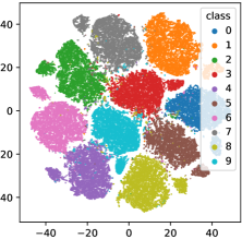
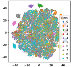
Figure 2: Visualization of t-SNE embeddings based on a target network’s output classification layer activations for Permuted MNIST in two scenarios. On the left hand, we used a target network weighted by a semi-binary mask (HyperMask). On the right side, we used only the target network without a mask produced by the hypernetwork. In the first case, data sample classes are separated; in the second case, only samples from the first task are distinguished.

Influence of semi-binary mask on classification task

The semi-binary mask of HyperMask helped the target network to discriminate classes in consecutive CL tasks. To visualize such properties, we considered Permuted MNIST dataset (results for other datasets we included in Appendix). We took the fully-trained model and collected activations of the output classification layer of the target network. In Fig. 2, we present t-SNE two-dimensional embeddings obtained from the classification layer for all data samples from 10 tasks. The evaluation was performed for an exemplary model that achieved $97.72\%$ mean overall accuracy after 10 CL tasks. The results for a tandem hypernetwork and target network (like in HyperMask) are presented on the left side. On the right side is shown a situation in which a mask from the hypernetwork was not applied to the target network trained in HyperMask. In the first case, data sample classes are clearly separated; in the second case, only samples from the first task are distinguished. The remaining data samples form one cluster in the embedding space. Interestingly, data from the first task are separated from samples from all subsequent tasks, which suggests that the first task plays a unique role in HyperMask.

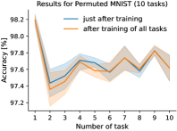
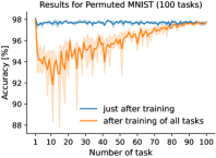
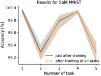
Figure 3: Visualization of mean accuracy (with 95% confidence intervals) for Permuted MNIST for 10 and 100 tasks and Split MNIST for 5 tasks. The blue lines represent test accuracy calculated after training consecutive models, while the orange lines correspond to test accuracy after finishing all CL tasks. The decrease in accuracy for 10-task Permuted MNIST and Split MNIST is minimal. The mean accuracy of the Permuted MNIST 100-task case equals $95.92\pm 0.18$.

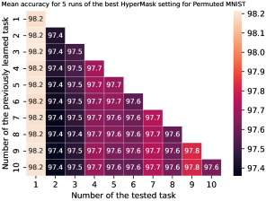
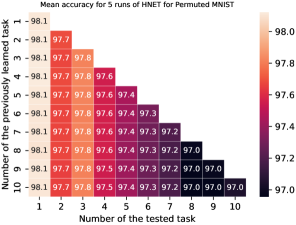
Figure 4: Mean test accuracy for consecutive CL tasks averaged over five runs of the best architecture settings of HyperMask (left side) and the default setting of HNET (right side) for ten tasks of Permuted MNIST dataset. Training of subsequent tasks leads to a slight decrease in the overall accuracy of the previous tasks, but, in general, HyperMask achieves higher accuracy for more recent tasks. However, HNET is more powerful for the first tasks.

Forgetting of previous tasks

The HNET models generate different masks for each task to minimize forgetting. we present in Fig. 3 mean accuracy (with 95% confidence intervals) for the best setting of HyperMask for ten tasks of Permuted MNIST dataset (left) and five tasks of Split MNIST dataset (right). The blue lines represent test accuracy calculated after training consecutive models, while the orange lines correspond to test accuracy after finishing all CL tasks. The accuracy decrease is minimal, and the confidence intervals almost overlap, suggesting limited negative backward transfer. In Fig. 4, we compare our HyperMask and HNET in terms of test accuracies for CL tasks after consecutive training sessions. Both methods suffer from performance drops only slightly. However, HyperMask is the most efficient for the initial and recent tasks, while HNET’s accuracy decreases smoothly with subsequent tasks.

Interestingly, HyperMask maintains accuracy on the first task, even after training on subsequent ones. Fig. 3 shows that for 100-task Permuted MNIST, HyperMask achieves similar test accuracy on the first task as just after its training even after training on 99 additional tasks. However, a drop in performance is observed, which is typical for continual learning methods. It may indicate that the hyper- and target network tandem is adapting to the first task, affecting weight behaviour.

We also examined HyperMask in terms of previous tasks’ forgetting for Tiny ImageNet. Fig. 5 depicts the test accuracies for subsequent CL tasks for the selected models of ResNet-20 and ZenkeNet target network architectures. The negative backward transfer was not substantial, and for some CL tasks, the accuracy even increased after gaining knowledge from the following tasks. The mean backward transfer was $-0.57$ for ResNet models and only $-0.13$ for ZenkeNet. A more detailed analysis of the specific cases of backward transfer is presented in Appendix A.

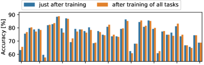
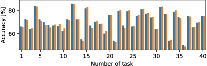
Figure 5: The accuracy of HyperMask for two models trained through 40 tasks on Tiny ImageNet. The first row presents results for a ResNet-20 model, with an accuracy of $75.87\%$, while the second row depicts scores of a ZenkeNet model, with an accuracy of $70.57\%$. Appendix A shows the results for all ten models.

Stability of HyperMask model

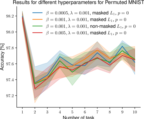
Figure 6: Visualization of stability of HyperMask. We obtained similar results for different hyperparameters.

HyperMask models have a similar number of hyperparameters as HNET. The most critical parameters are $\beta$ and $\lambda$, which control regularization strength. We also use a hyperparameter describing the level of zeros in a semi-binary mask, $p$, and define whether masked or non-masked $L_{1}$ must be used. Masked $L_{1}$ means that $\mathcal{L}_{target}$ was multiplied by the hypernetwork-generated mask while non-masked $L_{1}$ is the opposite case. In Fig. 6, we present mean test accuracy (with 95% confidence intervals) for five runs of the selected architecture settings of HyperMask, for ten tasks of Permuted MNIST dataset, calculated after training of all tasks. The results indicate slight hyperparameter changes do not impact performance. The blue line represents the best hyperparameter setting found.

Scenario with model’s task prediction

We also evaluated HyperMask in a scenario in which task identity is not directly given to the model but must be inferred by the network itself. Following von Oswald et al. (2019), we prepared a task inference method based on the entropy values (HyperMask + ENT). After training for all tasks, consecutive data samples were propagated through the hyper- and target network for different task embeddings. The task with the lowest entropy value of the classification layer’s output in the target network was selected for the final calculations. Then, the classifier decision for the corresponding embedding was considered. We also proposed a hybrid of HyperMask and FeCAM Goswami et al. (2023) in which HyperMask prepares features extraction and FeCAM creates task prototypes and selects a class based on HyperMask output. Initially, FeCAM worked on a feature extractor trained only on classes present in the first CL task, while in our case, FeCAM uses the output of HyperMask trained sequentially in all CL tasks.

Table 2: Mean overall accuracy (in $\%$) in a scenario where the model must recognize task identity. The results for two variants of HyperMask in the case of Split CIFAR-100 dataset are presented for the best model (max) and after averaging over five runs to enable a fair comparison with other methods. The results from other methods are derived from the paper on HNET von Oswald et al. (2019), marked with ^⋆, and FeCAM Goswami et al. (2023), marked with ^⋆⋆.

Method	Permuted MNIST	Split MNIST	Split CIFAR-100
				last task accuracy	average task accuracy HNET+ENT⋆	$91.75\pm 0.21$	$69.48\pm 0.80$		$-$	$-$
EWC⋆	$33.88\pm 0.49$	$19.96\pm 0.07$		$-$	$-$
SI⋆	$29.31\pm 0.62$	$19.99\pm 0.06$		$-$	$-$
DGR⋆	$96.38\pm 0.03$	$\mathbf{91.79\pm 0.32}$		$-$	$-$ Euclidean-NCM⋆⋆	$-$	$-$		$30.6$	$50.0$
FeTrIL⋆⋆	$-$	$-$		$46.2$	$61.3$
FeCAM⋆⋆	$-$	$-$		$48.1$	$62.3$ HyperMask+ENT (our)	$89.43\pm 1.49$	$62.89\pm 5.83$	(max)	$49.2$	$61.8$
			(5 runs)	$48.1\pm 0.76$	$61.1\pm 0.77$
HyperMask+FeCAM (our)	$\mathbf{97.03\pm 0.07}$	$83.28\pm 3.25$	(max)	$\mathbf{54.6}$	$\mathbf{65.8}$
			(5 runs)	$52.9\pm 1.00$	$64.5\pm 0.92$

Table 2 presents results for three datasets: Permuted MNIST (10 tasks), Split MNIST and CIFAR-100 (5 tasks per 20 classes, like in Table 5 in Goswami et al. (2023)). Even HyperMask + ENT achieved very competitive results, but HyperMask + FeCAM outperformed all baselines in Permuted MNIST and in a more demanding scenario with CIFAR-100. Both the last task and average task accuracy for HyperMask + FeCAM were higher than in the case of FeTrIL and FeCAM. Furthermore, even a more straightforward method, HyperMask + ENT, achieved comparable performance to other solutions. WSN in the paper Kang et al. (2022) only realizes the strategy in which the task identity is known in advance, and the authors did not describe a method for task inference. Therefore, we did not evaluate WSN in the above scenario. A detailed description of the HyperMask variants and considered scenarios are available in Appendix B.

Limitations and future works

One of the main limitations of HyperMask is the memory consumption because the hypernetwork output layer must have the same number of neurons as the number of parameters in the target network. The chunking approach described in von Oswald et al. (2019), in which the target’s weight values are generated by the hypernetwork partially, was not adopted in HyperMask because it led to considerably worse results so far. However, this approach should be analyzed thoroughly and may bring positive future results. It should facilitate taking advantage of larger architectures than ResNets.

5 Conclusion

We present HyperMask, a method that trains a single network for all tasks while the hypernetwork produces semi-binary masks to generate target subnetworks tailored to new tasks. This approach utilizes the hypernetwork’s capacity to adjust to new tasks with minimal forgetting. Also, due to the lottery ticket hypothesis, we can use a single network with weighted subnets devoted to each task.

The experimental section shows that our model obtains very competitive results compared to recent baselines and, in some cases, outperforms the state-of-the-art methods. HyperMask also has a potential for application for strategies in which task identity has to be inferred by the method.

Societal impact

This paper presents work whose goal is to advance the field of machine learning, especially continual learning. Our method may contribute to lowering the energy and time consumption necessary for retraining neural network models when new classes of data samples arrive.

Appendix A Appendix: Backward transfer

HNET models produce completely different weights for each task. In consequence, they demonstrate minimal forgetting. HyperMask models inherit such ability to minimize forgetting previous tasks thanks to masks created by hypernetworks. To measure the rate at which models forget previous tasks, we calculated a backward transfer (BWT) for the selected CL methods: WSN Kang et al. [2022], HNET von Oswald et al. [2019] and HyperMask. BWT measures forgetting previous tasks after learning the last one:

$$BWT=\frac{1}{T-1}\sum^{T-1}_{i=1}A_{T,i}-A_{i,i},$$

where $A_{T,i}$ is the test overall accuracy for task $i$ after training on task $T$, while $A_{i,i}$ is the test overall accuracy for task $i$ just after training the model on this task. Negative BWT means that learning new tasks caused the forgetting of past tasks. Zero BWT represents a situation where the accuracy of CL tasks did not change after gaining new knowledge. Finally, positive BWT corresponds to the state in which the model improved the accuracy of the previous CL tasks after learning the next tasks.

Table LABEL:tab:transfer presents mean backward transfer for five training runs of HNET+ENT and HyperMask for four experiments: Permuted MNIST with 10 or 100 tasks (for 100 tasks, three training runs were performed), Split MNIST and Tiny ImageNet datasets. By definition, WSN remembers masks from the preceding tasks. Therefore, the backward transfer, in this case, is always equal to zero. HNET and HyperMask achieved comparable and slightly negative values of BWTs for Permuted MNIST with 10 tasks and Split MNIST. In the case of Permuted MNIST with 100 CL tasks, we only have results for HyperMask. Despite a much larger number of tasks, the negative backward transfer did not exceed $2\%$. For a demanding Tiny ImageNet, HyperMask suffered only slightly from the negative backward transfer. ResNet obtained a bit higher rate of negative backward transfer than ZenkeNet, despite higher performance in terms of the mean classification accuracy (compare with Table 1). One of the five ResNet models trained on Tiny ImageNet achieved a backward transfer of $-0.03$ while one of the ZenkeNet models even obtained a positive backward transfer of $0.05$. The presented results suggest that HyperMask is largely immune to catastrophic forgetting.

[ caption = Mean backward transfer (in $\%$) with standard deviation for different continual learning methods.
^∗ denotes models trained with ResNet-20 while ^∗∗ with the reduced ZenkeNet architecture., label = tab:transfer, mincapwidth = doinside = , star = False, pos = h ]lccccDataset & Permuted MNIST Split MNIST Tiny ImageNet
10 tasks 100 tasks WSN, $c=30\%$ $0.0$ $-$ $-$ $0.0$
HNET+ENT $-0.018\pm 0.01$ $-$ $-0.027\pm 0.07$ $-$ HyperMask (our) $-0.025\pm 0.03$ $-1.791\pm 0.18$ $-0.009\pm 0.04$ $-0.574\pm 0.41^{*}$
 $-0.131\pm 0.15^{**}$

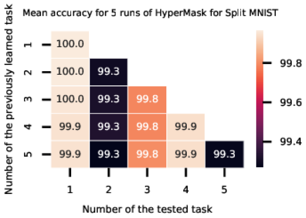
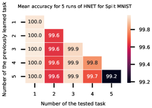
Figure 7: Mean test accuracy for consecutive CL tasks averaged over five runs of the best architecture settings of HyperMask (left side) and the default setting of HNET (right side) for 5 tasks of Split MNIST dataset. Similarly, as for Permuted MNIST, the performance drops after consecutive CL tasks are slight. Interestingly, the second and the last tasks (i.e., classification of numbers 2 and 3 or 8 and 9, respectively) are the most challenging for both methods.

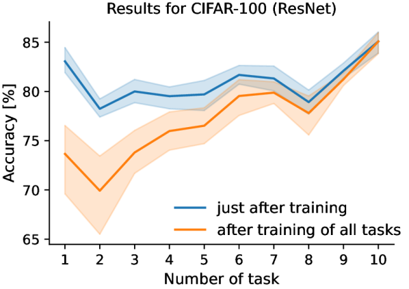
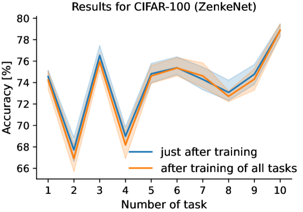
Figure 8: Visualization of mean accuracy (with 95$\%$ confidence intervals) of HyperMask for 10 tasks of CIFAR-100 dataset for two different target network architectures (ResNet-20 and ZenkeNet). The blue lines represent test accuracy calculated after training subsequent models, while the orange lines correspond to test accuracy after finishing training for all CL tasks. Even though ResNet-20 achieved higher accuracy than ZenkeNet, it suffers from catastrophic forgetting in a more severe way than the second considered architecture.

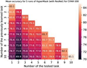
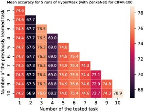
Figure 9: Mean test accuracy for consecutive CL tasks averaged over five runs of HyperMask for two target network architectures: ResNet-20 (left side) and ZenkeNet (right side) for ten tasks of CIFAR-100 dataset. For ZenkeNet, only a slight decrease in overall accuracy for previous tasks may be noticed, while for ResNet-20, there is a substantial drop in performance. However, the mean results are better for ResNet-20.

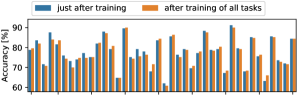
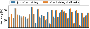
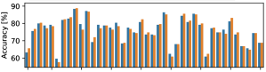
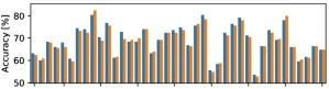
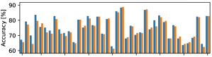
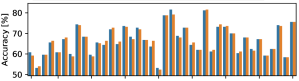
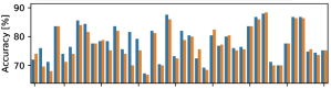
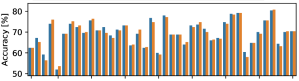
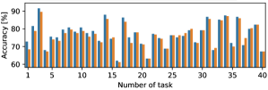
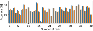
Figure 10: Visualization of the overall accuracy of HyperMask for all ten models trained through 40 CL tasks with samples from Tiny ImageNet dataset. The left column presents scores for ResNet-20 models that finally achieved $77.51$, $75.87$, $74.45$, $77.04$ and $76.24\%$ of mean task accuracy, respectively. ZenkeNet models, shown in the second column, were slightly less performing ($70.57$, $68.52$, $66.79$, $69.39$ and $70.40\%$ of mean task accuracy, respectively). Because the order of classes was randomly selected for each training run, it was impossible to present one graph for five models of a given architecture (with mean and confidence intervals defined per task). The models worked on differently constructed tasks. However, models from a given row may be compared to each other because the task and class settings were, in such a case, the same.

A.1 Analysis of consecutive CL tasks

In the main work, we selected Permuted MNIST dataset to visualize performance drop after learning subsequent CL tasks by HyperMask and HNET, see Fig. 4. We show analogical results on Split MNIST in Fig. 7. Both methods feature minimal forgetting after training on consecutive tasks. The situation changes when we consider a more demanding dataset like Split CIFAR-100, see Figs. 8-9. ZenkeNet, despite lower classification accuracy than ResNet-20, achieved only a slight decrease in performance after succeeding tasks. In the case of ResNet-20, the drop in efficiency was considerable, for instance, from $83.1\%$ just after learning of the first task to $73.7\%$ at the end of the CL scenario. However, a more intense regularization (i.e. higher values of $\beta$ and $\lambda$), that may prevent the network from knowledge forgetting, led to slightly lower mean accuracy averaged over ten tasks. Therefore, a final hyperparameter choice has to be a compromise. For another dataset, for which convolutional neural networks were selected as target networks, i.e. Tiny ImageNet, knowledge forgetting was not as noticeable as for Split CIFAR-100. Such analysis is presented in Fig. 10. By comparing accuracy just after training of consecutive tasks with the final accuracy, it can be concluded that for most tasks, there was only a minor performance decrease. However, as for Split CIFAR-100, ZenkeNet models suffered less from catastrophic forgetting than the ResNet ones. The most considerable forgetting was for the fourth ResNet model, where the overall accuracy for task no. 14 dropped from 81.6 to 70%. In many cases, even a small increase in efficiency may be denoted. For instance, for task no. 26 of the same model, the accuracy increased from 76.8 to 77.2%. Also, the classification of the ninth task in the case of the second ZenkeNet training run has been improved (from 80.4 to 82.4%).

Appendix B Appendix: Architecture details

We implemented HyperMask in Python 3.7.16 with the use of such libraries like hypnettorch 0.0.4 von Oswald et al. [2019], PyTorch 1.5.0, NumPy 1.21.6, Pandas 1.3.5, Matplotlib 3.5.3, seaborn 0.12.2 and others. Network training sessions were performed using NVIDIA GeForce RTX 2070 and NVIDIA GeForce RTX 2080 Ti graphic cards.

We tried to implement hypernetwork and target network architectures close to the work presenting HNET algorithm von Oswald et al. [2019], but we performed an intensive grid search optimization for some hyperparameters, especially those present only in HyperMask. In all cases, we did not use chunked hypernetworks, i.e. we did not generate a mask in small pieces. It means that the hypernetwork output layer always had the same number of neurons, like the number of weights of the target network. It is because each output neuron produces a single value of the mask for the corresponding target network’s weight. This solution is more memory expensive than the chunking approach, but, currently, in the case of HyperMask, it ensures higher classification accuracy.

Permuted MNIST

Final experiments on Permuted MNIST dataset with 10 CL tasks were performed using the following architecture. The hypernetwork had two hidden layers with 100 neurons per each. The target network was selected as a multilayer perceptron with two hidden layers of 1000 neurons and ELU activation function with $\alpha$ hyperparameter regarding the strength of the negative output equaling 1. The size of the embedding vectors was set to 24. The sparsity parameter $p$ was adjusted to 0, and the regularization hyperparameters were as follows: $\beta=0.0005$ and $\lambda=0.001$. Furthermore, a masked $L_{1}$ regularization was chosen. The training of models was performed through 5000 iterations with a batch size of $128$ and Adam optimizer with a learning rate set to $0.001$. Finally, models after the last training iterations were selected. The validation set consisted of 5000 samples. The data was not augmented. The presented results are averaged over five training runs for different seed values. Also, the dataset was padded with zeros, and the MNIST images’ final size was $32\times 32$.

For 100 CL tasks, the hyperparameters were the same as above, but three training runs were performed.

To select the best hyperparameter set, we performed an intensive hyperparameter optimization. In the final stage, we evaluated, in different configurations, various hypernetwork settings ($[25,25],[100,100]$), masked and non-masked $L_{1}$ regularization, $p\in\{0,30\}$, $\beta\in\{0.0005,0.001,0.0025,0.005,0.01,0.1\}$ and $\lambda\in\{0.0005,0.001,0.0025,0.005,0.01\}$.

In the initial experiments, we also considered hypernetworks having two hidden layers with 50 neurons per each, embeddings of sizes 8 and 72, a learning rate of $0.0001$, batch size of $64$, $\beta=0.05$, $\lambda\in\{0.0001,0.00001,0.05\}$ and $p=70$.

Split MNIST

For this dataset with 5 CL tasks, we applied data augmentation and trained models through 2000 iterations. The best-performing model comprised a hypernetwork with two hidden layers with 25 neurons per each and a target network with two hidden layers consisting 400 neurons. We used $\beta=0.001$ and a sparsity parameter $p=30$. Furthermore, the embedding size was 128. In each task, 1000 samples were assigned to the validation set. The rest of the hyperparameters were the same as for Permuted MNIST, i.e. we applied a masked $L_{1}$ regularization with $\lambda=0.001$, ELU activation function with $\alpha=1$, Adam optimizer with a learning rate of $0.001$ and batch size of $128$. Also, the mean results are averaged over five training runs.

During the hyperparameter optimization stage, we evaluated models with embedding sizes of $24,72,96$ and $128$, hypernetworks with hidden layers of shapes $[10,10],[25,25]$ and $[50,50]$, masked and non-masked $L_{1}$ regularization, batch sizes of $64$ and $128$, $\beta\in\{0.001,0.01\}$, $p\in\{0,30,70\}$ and $\lambda\in\{0.0001,0.001\}$.

CIFAR-100

Known task identity

In this dataset, we assumed 10 tasks with 10 classes per each (classes 1-10, 11-20, …, 91-100). Another version of this CL benchmark adopts CIFAR-10 and 5 tasks (i.e., 50 classes) of CIFAR-100 dataset, like in von Oswald et al. [2019]. However, we selected the first scenario, similarly as in Kang et al. [2022].

We performed experiments for two different convolutional target networks: ResNet-20 and ZenkeNet. The first is similar to the network considered in von Oswald et al. [2019] but is slightly shorter, while the second is more similar to AlexNet used in Kang et al. [2022]. ZenkeNet is even less sophisticated architecture than AlexNet.

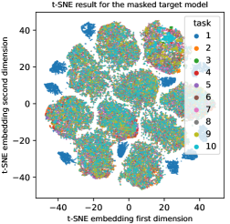
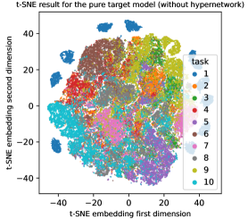
Figure 11: t-SNE embeddings of features extracted from all data samples of 10 tasks of Permuted MNIST dataset, created similarly as embeddings presented in Fig. 2, but the samples are labelled relative to the CL tasks. On the left column, results for HyperMask (i.e. hypernetwork and target network) are shown. On the right column are presented only results for the target network, without the application of a mask from hypernetwork. The plots clearly indicate that samples from the first task form a separate structure in the data space. Even when the classical version of HyperMask is used, the first task plays a particular role.

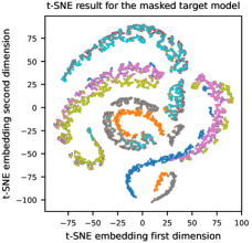
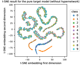
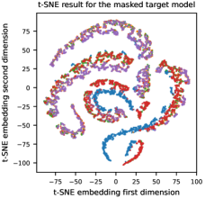
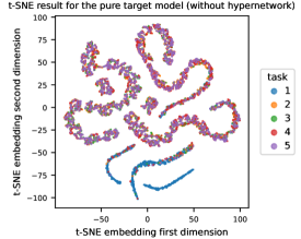
Figure 12: t-SNE embeddings of features extracted from all data samples of 5 tasks of Split MNIST dataset. Values were taken from the classification layer of the target network for an exemplary model that achieved $99.76\%$ overall accuracy after 5 CL tasks. The results for a tandem hypernetwork and target network (like in HyperMask) are presented on the left column. On the right column is shown a mask from hypernetwork that was not applied to the target network while it was trained in tandem in HyperMask. In the first case, classes form different clusters, especially the pairs of classes which were mutually compared in consecutive CL tasks (0 and 1, 2 and 3, etc.). In the second case, only 0s and 1s are separated while the remaining data samples are mixed in the embedding subspace. Furthermore, in this situation, data from the first task form a separate cluster, which suggests that it mainly defines the structure of the data space.

In more detail, we selected a ResNet architecture containing 20 layers with 9 residual blocks and a widening factor equal to 2, doubling the convolutional filters. During the hyperparameter optimization, we also considered a narrower architecture as well as shorter and longer ResNets (up to 32 layers), but they were less promising than a 20-layer network. Also, batch normalization was used (these layers were excluded from multiplying by hypernetwork-based masks). Batch statistics were calculated even during the evaluation, i.e. parameters were not stored after consecutive CL tasks.

ZenkeNet is a convolutional neural network described in Zenke et al. [2017]. It consists of two blocks of two convolutional layers containing 32 and 64 filters, respectively. A single max pooling layer finishes each block. Finally, the network has two fully connected layers with 512 and 10 neurons, respectively.

During the hyperparameter optimization for ZenkeNet, we used models having embedding size set to 48, a hypernetwork with one hidden layer with 100 neurons, trained with Adam optimizer using a learning rate of 0.001 and batch size of 32. A non-masked $L^{1}$ regularization was selected as the more promising. Furthermore, we evaluated $\beta\in\{0.01,0.1,1\}$ and $\lambda\in\{0.01,0.1,1\}$. The sparsity parameter $p$ was set to 0. Also, a learning rate scheduler was applied, i.e. after five consecutive epochs without improvement, the learning rate was multiplied by $\sqrt{0.1}$. In the case of ZenkeNet, for the final experiments, $\beta=0.01$ and $\lambda=0.01$ were selected.

For the ResNet, most of the hyperparameters were the same as for ZenkeNet, excluding $\lambda=1$.

For both considered networks, the dataset was augmented according to the approach implemented in the hypnettorch library. In the validation set of each task, there were 500 samples. It is worth emphasizing that the lack of data augmentation led to significantly lower accuracy than in the opposite case. The network training was performed through 200 epochs, and the best model was chosen based on the validation loss.

Unknown task identity

In this scenario, we followed the setting from Goswami et al. [2023] to ensure a representative comparison of methods. The order of classes present in CIFAR-100 was mixed, and we followed the order described in the FeCAM source code. Then, 100 classes were divided into five tasks, with 20 classes per each. This class incremental setting corresponds to the results from Table 5 depicted in Goswami et al. [2023]. We also followed the accuracy calculation approach from this work, which is different than in the previously described experiments in our paper. Therefore, average task accuracy presented in Table 2 in Section 4 is calculated as follows:

$$\mathrm{AVG}=\frac{1}{5}\sum\limits_{j=1}^{5}\mathrm{Acc_{j}},$$

where $\mathrm{Acc_{j}}$ represents the overall accuracy for the test samples from tasks $\{1,2,...,j\}$ after creating class prototypes from the $j$–th task. The last task accuracy just refers to $\mathrm{Acc_{5}}$, which is calculated for the test set containing samples from all 100 classes after the fifth task.

Furthermore, we present results for the best-trained model as well as for 5 different runs with the same hyperparameters and the given order of CIFAR-100 classes.

In this case, we only performed experiments with ResNet architecture with the same layer setting as for the case with known task identity. However, we slightly changed some network hyperparameters. For HyperMask + FeCAM, we selected a hypernetwork with one hidden layer with 200 neurons, trained with a lower initial learning rate set to 0.0001. The rest of the hyperparameters were exactly the same as for ResNet with a known task identity setting. During forward propagation through ResNet in the FeCAM evaluation stage, we set a batch size to 2000. Due to batch normalization in ResNet, this hyperparameter also affects the results. We selected 2000 due to the higher scores and the fact that the test set in each task consists of 2000 samples.

We also evaluated the model for some additional hyperparameter values, i.e. for the hypernetwork with one hidden layer with 100 neurons, the learning rate set to 0.001 or 0.01, and for the embedding of sizes 24 or 96.

The augmentation of the dataset was performed in a different way than for the known task identity setting. In this setup, we followed the more sophisticated approach from FeCAM.

Tiny ImageNet

In this case, we divided the dataset randomly into 40 tasks with five classes, similarly to Kang et al. [2022]. We assumed the same training strategy, i.e. we learned each task through 10 epochs, and the validation set consisted of 250 samples. We performed experiments with ResNet-20 architecture, explained in detail in the section devoted to CIFAR-100. However, in WSN Kang et al. [2022], La-MaML Gupta et al. [2020] and FS-DPGM Deng et al. [2021] authors used an architecture with four convolutional and three fully connected layers. The best models were chosen according to the values of the validation loss. We augmented the dataset using random cropping and horizontal flipping. For the hypernetwork, we selected a multilayer perceptron with two hidden layers of 100 neurons while the task embedding vector size was set to 96. Furthermore, we used non-masked $L_{1}$ regularization with $\beta=1$ and $\lambda=0.1$. Also, the sparsity parameter $p$ was adjusted to 0. We performed training with Adam optimizer with a batch size 16 and a learning rate 0.0001. The learning rate scheduler was the same as for CIFAR-100, i.e. a patience step was equal to 5 epochs, and the multiplication factor was $\sqrt{0.1}$.

In the hyperparameter optimization stage, we considered an order of magnitude greater learning rate, i.e. 0.001, like in Kang et al. [2022], but it led to weaker results. Also, other sizes of embedding vectors, consisting of 48 and 128 coordinates, were verified, but the most outstanding performance was achieved for 96. Similarly, smaller hypernetworks, i.e., those consisting of two hidden layers with 10 neurons or one hidden layer with 100 neurons, were rejected. We also tested a masked $L_{1}$ regularization and lower values of $\beta$ and $\lambda$, but stronger regularization is preferred for this target network architecture and such a complicated dataset. For some solutions, $p=30$ led to better solutions than $p=0$, but finally, we selected $p=0$.

We also conducted experiments for a simpler architecture than ResNet-20, i.e. ZenkeNet. The only difference in its structure between the setting for CIFAR-100 and Tiny ImageNet was the lack of a fully connected layer having 512 neurons. For the final experiments, we selected a hypernetwork of two hidden layers with 100 neurons per layer and an embedding size set to 96. Each task was trained through 10 epochs with a learning rate of 0.001, a batch size of 16 and 250 validation samples. We used non-masked $L_{1}$ regularization, and we set a sparsity parameter $p$ to 50. We also chose $\beta=0.01$ and $\lambda=1$.

The above hyperparameters were selected based on a series of experiments with embedding sizes of 96, 128 and 192, sparsity parameters of 0, 30 and 50, learning rates of 0.0001, 0.001 and 0.005, as well as $\beta$ and $\lambda$ values were selected among 0.001, 0.01, 0.1 and 1.

Appendix C Appendix: Influence of semi-binary mask on classification task

In the main paper, we showed that the semi-binary mask of HyperMask helps the target network to discriminate classes in consecutive CL tasks. We considered Permuted MNIST dataset to visualize such properties (see Fig. 2). Now, in Fig. 11, we present plots for this dataset with data samples labelled according to the CL task and results for Split MNIST in Fig. 12. Interestingly, even when the mask was not applied, the first task was solved correctly, and the corresponding samples formed separate clusters. Furthermore, data from the first task form a separate structure in the embedding subspace, even when just the target network is applied. It suggests that the first task is critical during training of HyperMask with target networks being multilayer perceptrons. This observation is supported by the results presented in Fig. 3, where the classification accuracy for the first task remains high despite learning many subsequent CL tasks.

Appendix D Appendix: Classification with task identity recognition

D.1 HyperMask + ENT

HyperMask + ENT is a simple method where task recognition is based on a minimization of an entropy criterion calculated on network logits’ outputs. A similar approach has been used in HNET von Oswald et al. [2019] for strategies in which task identity was identified without the generation of additional data samples. The consecutive steps of this method are summarized in Algorithm 2.

Let us assume that we have a hypernetwork $\mathcal{H}$ with weights $\bm{\Theta}$ and a target network $f$ with weights $\bm{\theta}$, trained according to Algorithm 1. Depending on the considered scenario, we can evaluate the method after finishing the training of all $T$ tasks or just after one of the previous tasks, $t$, where $t\in\{1,2,...,T\}$. In the second case, we only predict the samples that may belong to one of the classes $\{1,2,...,t\}$.

In the general case, we suppose that HyperMask was trained on $t$ tasks, and we have to classify a test sample $\bm{x}$. Using embeddings designed for all possible tasks, we perform forward propagation through the hyper- and target network to get logits of the output classification layer. In the next step, we apply the softmax function to obtain a vector of predictions in which single values range from 0 to 1, according to the following equation:

$$\bm{\psi}_{i}(\bm{x})=\mathrm{Softmax}\big{(}f\big{(}\bm{x},\mathcal{H}(\bm{e}_{i},\Phi)\big{)}\big{)},$$

where $\bm{e}_{i}$ is the embedding of the $i$–th task. Therefore, we obtain $t$ vectors of HyperMask predictions: $\big{(}\bm{\psi}_{1}(\bm{x}),\bm{\psi}_{2}(\bm{x}),...,\bm{\psi}_{t}(\bm{x})\big{)}$. Then, for such vectors, we calculate the entropy criterion:

$$\psi_{i}^{ENT}(\bm{x})=-\sum\nolimits_{j=1}^{C}\big{(}\psi_{i}(\bm{x})[j]\cdot\log\big{(}\psi_{i}(\bm{x})[j]\big{)}\big{)},$$

where $C$ is the number of classes. Now, we have values corresponding to each of $t$ tasks: $\big{(}\psi_{1}^{ENT}(\bm{x}),\psi_{2}^{ENT}(\bm{x}),...,\psi_{t}^{ENT}(\bm{x})\big{)}$. We select a task that minimizes the entropy criterion:

$$t^{\star}=\operatorname*{arg\,min}\limits_{i=1,2,...,t}\big{(}\psi_{i}^{ENT}(\bm{x})\big{)}.$$

Finally, we choose the class with the highest softmax value and assign it as the label for sample $x$:

$$c^{\star}=\operatorname*{arg\,max}\limits_{j=1,2,...,C}\big{(}\psi_{t^{\star}}(\bm{x})[j]\big{)}.$$

Algorithm 2 The pseudocode of HyperMask+ENT.

trained hypernetwork $\mathcal{H}$ with weights $\bm{\Phi}$, including embeddings $(\bm{e}_{1},\bm{e}_{2},...,\bm{e}_{T})$; trained target network $f$ with weights $\bm{\theta}$; test samples $\bm{X}_{test}^{t}$; selected task $t$, where $t\in\{1,2,...,T\}$; number of classes $C$

predictions for test samples $\bm{\hat{Y}}_{test}^{t}$

for $\bm{x}\in\bm{X}_{test}^{t}$ do

     for $i\in\{1,2,...,t\}$ do

         $\bm{\psi}_{i}(\bm{x})=\mathrm{Softmax}\big{(}f\big{(}\bm{x},\mathcal{H}(\bm{e}_{i},\Phi)\big{)}\big{)}$

         $\psi_{i}^{ENT}(\bm{x})=-\sum\nolimits_{j=1}^{C}\big{(}\psi_{i}(\bm{x})[j]\cdot\log\big{(}\psi_{i}(\bm{x})[j]\big{)}\big{)}$

     end for

     $t^{\star}=\operatorname*{arg\,min}\limits_{i=1,2,...,t}\big{(}\psi_{i}^{ENT}(\bm{x})\big{)}$

     $c^{\star}=\operatorname*{arg\,max}\limits_{j=1,2,...,C}\big{(}\psi_{t^{\star}}(\bm{x})[j]\big{)}$

end for

D.2 HyperMask + FeCAM

HyperMask + FeCAM is a hybrid method which combines the advantages of these two approaches. HyperMask is trained similarly to the basic case, but then it is used as the feature extractor while FeCAM assigns a label based on the HyperMask output. Initially, in FeCAM Goswami et al. [2023], the feature extractor was not trained after the first task. We propose this strategy for cases where task identities are unknown. The pseudocode of this method is depicted in Algorithm 3 and now will be described in detail.

Similar to HyperMask + ENT, let us suppose that we have a hypernetwork $\mathcal{H}$ with weights $\bm{\Theta}$ and a target network $f$ with weights $\bm{\theta}$, trained according to Algorithm 1. During the evaluation phase of the $t$–th task, where $t\in\{1,2,...,T\}$ and $T$ is the total number of tasks, we have to prepare class prototypes based on train samples belonging to consecutive classes present in all previous tasks, up to the $t$-th task. In practice, we can just update the set of prototypes in subsequent tasks. There is no need to recalculate prototypes from the preceding tasks if no new samples from previously known classes exist.

In the beginning, for each element of the training dataset, we extract the output of the hidden layers of the target network after forward propagation (just before the last fully connected layer). It means that for the samples from the $t$–th task, we prepare features extraction:

$$\bm{\tilde{X}}^{t}=f\big{(}\bm{X}_{train}^{t},\mathcal{H}(\bm{e}_{t},\Phi)\big{)}.$$

Based on such prepared features, for each class from the training set, we calculate its prototype as an average of all samples belonging to this class:

$$\bm{\mu}_{c}=\frac{1}{|\bm{X}_{c}|}\sum\limits_{\bm{x}\in\bm{X}_{c}}\bm{x},$$

where $\bm{X}_{c}$ represents features calculated for all training samples from the $c$–th class while $|\bm{X}_{c}|$ is the number of these samples. We also have to calculate a covariance matrix, which has to be invertible. Similar to FeCAM Goswami et al. [2023], we apply a covariance shrinkage according to the following equation:

$$(\bm{\Sigma}_{c})_{s}=\bm{\Sigma}_{c}+D_{1}\bm{I}+D_{2}(\bm{1}-\bm{I}),$$

where $\bm{\Sigma}_{c}$ is the covariance matrix, $D_{1}$ is the mean value of all diagonal elements of $\bm{\Sigma}_{c}$, while $D_{2}$ is the mean value of the elements lying outside the main diagonal of $\bm{\Sigma}_{c}$. Also, $\bm{I}$ is the identity matrix, and $\bm{1}$ is the matrix filled with ones.

In HyperMask+FeCAM, the covariance shrinkage is performed twice. Furthermore, contrary to FeCAM, we skip using Tukey’s Ladder of Powers transformation due to worse performance. Finally, we normalize the covariance matrix:

$$(\tilde{\bm{\Sigma}}_{c})_{s}[i,j]=\dfrac{({\bm{\Sigma}}_{c})_{s}[i,j]}{\sqrt{({\bm{\Sigma}}_{c})_{s}[i,i]}\cdot\sqrt{({\bm{\Sigma}}_{c})_{s}[j,j]}},$$

where $({\bm{\Sigma}}_{c})_{s}[i,j]$ corresponds to the element of the shrunken covariance matrix located at position $[i,j]$.

When all class prototypes are determined, one can start evaluating the test set. Therefore, for a given test sample $\bm{x}$, it is necessary to collect the network output for each embedding $\bm{e}_{i}$, where $i\in\{1,2,...,t\}$, and $t$ is the number of the last trained task:

$$\bm{\phi}_{i}(\bm{x})=f\big{(}\bm{x},\mathcal{H}(\bm{e}_{i},\Phi)\big{)}.$$

As before, we use features from the last hidden layer of HyperMask, not the output of the classification layer. Then, we must calculate the squared Mahalanobis distance between all classes and network outputs. Therefore, such a distance between features created by HyperMask with the $i$–th embedding and the $c$–th class prototype is defined in the following way:

$$d_{M}\big{(}\bm{\phi}_{i}(\bm{x}),\bm{\mu}_{c}\big{)}=\bigg{(}\frac{\bm{\phi}_{i}(\bm{x})}{\lVert\bm{\phi}_{i}(\bm{x})\rVert_{2}}-\frac{\bm{\mu}_{c}}{\lVert\bm{\mu}_{c}\rVert_{2}}\bigg{)}^{\top}(\tilde{\bm{\Sigma}}_{c})^{-1}_{s}\bigg{(}\frac{\bm{\phi}_{i}(\bm{x})}{\lVert\bm{\phi}_{i}(\bm{x})\rVert_{2}}-\frac{\bm{\mu}_{c}}{\lVert\bm{\mu}_{c}\rVert_{2}}\bigg{)},$$

where $(\tilde{\bm{\Sigma}}_{c})^{-1}_{s}$ is the inverse of a normalized covariance matrix. Vectors of features and class prototypes are also normalized. Finally, one needs just to choose the class whose prototype is the closest to the given sample representation:

$$c^{\star}=\operatorname*{arg\,min}\limits_{c=1,2,...,|\bm{\mu}|}\bigg{(}\min\limits_{i=1,2,...,t}d_{M}\left(\bm{\phi}_{i}(\bm{x}),\bm{\mu}_{c}\right)\bigg{)},$$

where $|\bm{\mu}|$ is the number of classes (and corresponding prototypes).

Algorithm 3 The pseudocode of HyperMask+FeCAM.

trained hypernetwork $\mathcal{H}$ with weights $\bm{\Phi}$, including embeddings $(\bm{e}_{1},\bm{e}_{2},...,\bm{e}_{T})$; trained target network $f$ with weights $\bm{\theta}$; training datasets $(D_{train}^{1},D_{train}^{2},...,D_{train}^{T})$, $(\bm{X}_{train}^{i},\bm{Y}_{train}^{i})\in D_{train}^{i},$ $i\in\{1,...,T\}$; test samples $(\bm{X}_{test}^{1},\bm{X}_{test}^{2},...,\bm{X}_{test}^{T})$

predictions for test samples $(\bm{\hat{Y}}_{test}^{1},\bm{\hat{Y}}_{test}^{2},...,\bm{\hat{Y}}_{test}^{T})$

for $t\leftarrow 1$ to $T$ do

     for $i\leftarrow 1$ to $t$ do

         $\bm{\hat{X}}^{i}=f\big{(}\bm{X}_{train}^{i},\mathcal{H}(\bm{e}_{i},\Phi)\big{)}$

     end for

     $\bm{\tilde{X}}^{t}=\bm{\hat{X}}^{1}\cup\bm{\hat{X}}^{2}\cup...\cup\bm{\hat{X}}^{t}$

     $\bm{\tilde{Y}}^{t}=\bm{Y}_{train}^{1}\cup\bm{Y}_{train}^{2}\cup...\cup\bm{Y}_{train}^{t}$

     for $c\in\bm{\tilde{Y}}^{t}$ do

         Select samples belonging to the $c$–th class, $\bm{X}_{c}$, from $\bm{\tilde{X}}^{t}$

         $\bm{\mu}_{c}=\frac{1}{|\bm{X}_{c}|}\sum\limits_{\bm{x}\in\bm{X}_{c}}\bm{x}$

         $\bm{\Sigma}_{c}=\mathrm{Covariance}(\bm{X}_{c})$

         $(\bm{\Sigma}_{c})_{s}=\mathrm{Shrinkage}\big{(}\mathrm{Shrinkage}(\bm{\Sigma}_{c})\big{)}$

         $(\tilde{\bm{\Sigma}}_{c})_{s}=\mathrm{Normalize}(\bm{\Sigma}_{c})_{s}$

     end for

     for $\bm{x}\in\bm{X}_{test}^{t}$ do

         for $i\in\{1,2,...,t\}$ do

              $\bm{\phi}_{i}(\bm{x})=f\big{(}\bm{x},\mathcal{H}(\bm{e}_{i},\Phi)\big{)}$

              for $c\in\bm{\hat{Y}}_{train}^{t}$ do

                  $d_{M}\left(\bm{\phi}_{i}(\bm{x}),\bm{\mu}_{c}\right)=\big{(}\frac{\bm{\phi}_{i}(\bm{x})}{\lVert\bm{\phi}_{i}(\bm{x})\rVert_{2}}-\frac{\bm{\mu}_{c}}{\lVert\bm{\mu}_{c}\rVert_{2}}\big{)}^{\top}(\tilde{\bm{\Sigma}}_{c})^{-1}_{s}\big{(}\frac{\bm{\phi}_{i}(\bm{x})}{\lVert\bm{\phi}_{i}(\bm{x})\rVert_{2}}-\frac{\bm{\mu}_{c}}{\lVert\bm{\mu}_{c}\rVert_{2}}\big{)}$

              end for

         end for

         $c^{\star}=\operatorname*{arg\,min}\limits_{c=1,2,...,|\bm{\mu}|}\bigg{(}\min\limits_{i=1,2,...,t}d_{M}\left(\bm{\phi}_{i}(\bm{x}),\bm{\mu}_{c}\right)\bigg{)}$

     end for

end for

Appendix E Appendix: Stability of HyperMask model

HyperMask model has a similar number of hyperparameters as HNET. The most critical ones are $\beta$ and $\lambda$, which control regularization strength. This method also has a hyperparameter $p$ describing the level of zeros in consecutive layers of the semi-binary mask. Moreover, we define whether or not $L_{1}$ loss is additionally multiplied by the hypernetwork-generated mask values. Furthermore, similarly to HNET, there exists another branch of hyperparameters regarding the networks’ shape, for instance, the hypernetwork embedding size, the number of hidden layers and the number of neurons in consecutive layers. Similarly, we have to define the setting of the target network.

In Fig. 13, we present mean test accuracy for consecutive CL tasks averaged over two runs of different architecture settings of HyperMask for five tasks of Split MNIST dataset. Most of the HyperMask models achieve the highest classification accuracy for the first CL task while the weakest one for the subsequent tasks. In all of the above plots, results are compared with the best hyperparameter setting, i.e. with an embedding size of 128, a hypernetwork having two hidden layers with 25 neurons per each, $\beta=0.001$, $\lambda=0.001$, $p=30$, a batch size of 128 and masked $L^{1}$ norm. In consecutive subplots, some of the above hyperparameters are changed, and the performance of corresponding models is compared with the most efficient setup.

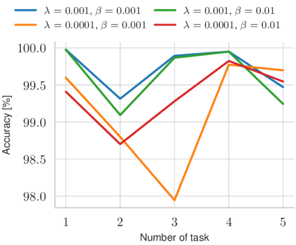
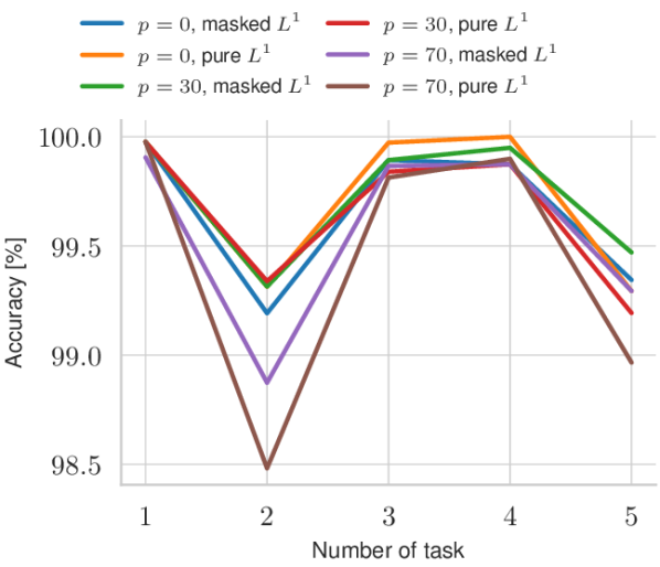
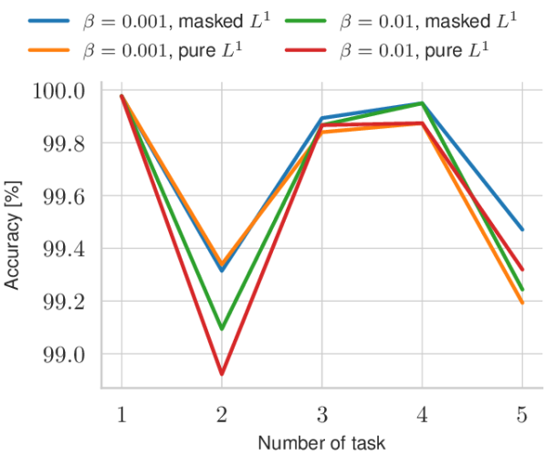
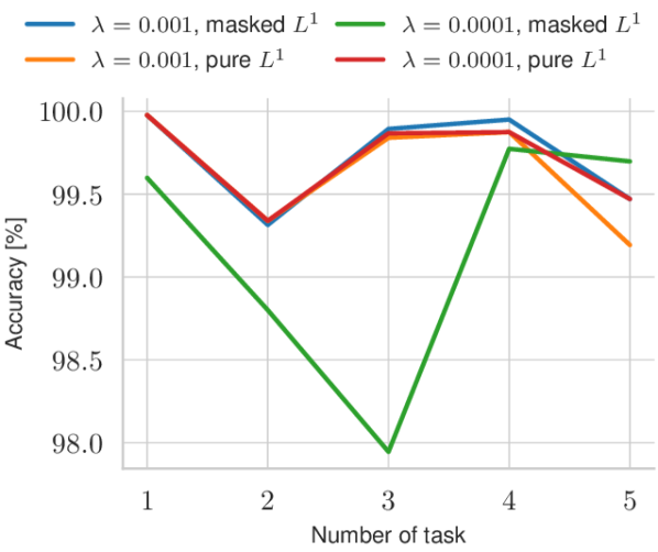
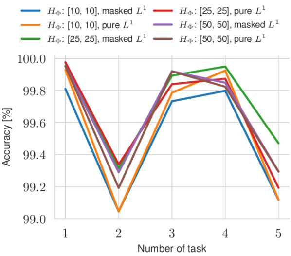
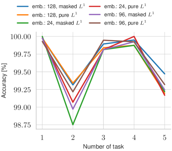
Figure 13: Mean test accuracy for consecutive CL tasks averaged over two runs of different architecture settings of HyperMask for five tasks of Split MNIST dataset. Most of the HyperMask models achieve the highest classification accuracy for the first CL task while the weakest one for the subsequent task. In many cases, differences in performance of the compared models are slight.

Appendix F Appendix: Time consumption

We depicted in Tab. LABEL:tab:calculation the mean training time of HyperMask for five tasks of Split MNIST, ten tasks of Permuted MNIST, ten tasks of Split CIFAR-100 and forty tasks of Tiny ImageNet using NVIDIA GeForce RTX 2070 and NVIDIA GeForce RTX 2080 Ti graphic cards. For the easiest dataset, HyperMask needs only slightly more than 21 minutes. In the case of Permuted MNIST, which consists of more advanced CL tasks, HyperMask needs less than 2 hours. For Split CIFAR-100 and more complicated convolutional architectures, calculation times are higher: about 6 hours for ZenkeNet and more than 10 hours for ResNet-20. However, it is necessary to remember that each of the 10 CL tasks was trained through 200 epochs. Another dataset, i.e. Tiny ImageNet, contains images having larger spatial resolution than CIFAR-100 ($64$ instead of $32$). Each of the 40 five-class CL tasks was learned only through 10 epochs. Therefore, calculation times are substantially lower than in the previous case. For ResNet-20, it is about 4 hours less in favour of Tiny ImageNet, while for a slightly reduced ZenkeNet (details about a difference in Appendix B), time is about four times smaller. It would be even shorter if the time necessary for loading the dataset and creating 40 tasks would not be considered (over a dozen minutes).

[ caption = Mean training time of HyperMask for different datasets., label = tab:calculation, mincapwidth = doinside = , star = False, pos = h ]llDataset Mean calculation time in HH:MM:SS (with standard deviation) Split MNIST 00:21:06 $\pm$ 00:02:37
Permuted MNIST 01:45:14 $\pm$ 00:04:07
Split CIFAR-100 (ZenkeNet) 06:02:25 $\pm$ 00:01:54
Split CIFAR-100 (ResNet-20) 10:26:37 $\pm$ 00:10:05
Tiny ImageNet (ZenkeNet) 01:29:10 $\pm$ 00:01:23
Tiny ImageNet (ResNet-20) 06:39:23 $\pm$ 00:25:13

References

- Chen et al. (2020) T. Chen, Z. Zhang, S. Liu, S. Chang, and Z. Wang. Long live the lottery: The existence of winning tickets in lifelong learning. In International Conference on Learning Representations, 2020.
- De Lange et al. (2021) M. De Lange, R. Aljundi, M. Masana, S. Parisot, X. Jia, A. Leonardis, G. Slabaugh, and T. Tuytelaars. A continual learning survey: Defying forgetting in classification tasks. IEEE transactions on pattern analysis and machine intelligence, 44(7):3366–3385, 2021.
- Deng et al. (2021) D. Deng, G. Chen, J. Hao, Q. Wang, and P.-A. Heng. Flattening sharpness for dynamic gradient projection memory benefits continual learning. Advances in Neural Information Processing Systems, 34:18710–18721, 2021.
- Frankle and Carbin (2018) J. Frankle and M. Carbin. The lottery ticket hypothesis: Finding sparse, trainable neural networks. In International Conference on Learning Representations, 2018.
- Golkar et al. (2019) S. Golkar, M. Kagan, and K. Cho. Continual learning via neural pruning. arXiv preprint arXiv:1903.04476, 2019.
- Goswami et al. (2023) D. Goswami, Y. Liu, B. Twardowski, and J. van de Weijer. Fecam: Exploiting the heterogeneity of class distributions in exemplar-free continual learning. In Advances in Neural Information Processing Systems (NeurIPS), 2023.
- Gupta et al. (2020) G. Gupta, K. Yadav, and L. Paull. La-maml: Look-ahead meta learning for continual learning. In Proceedings of the 34th International Conference on Neural Information Processing Systems, NIPS’20, Red Hook, NY, USA, 2020. Curran Associates Inc. ISBN 9781713829546.
- Ha et al. (2016) D. Ha, A. Dai, and Q. V. Le. Hypernetworks. arXiv preprint arXiv:1609.09106, 2016.
- Henning et al. (2021) C. Henning, M. Cervera, F. D’Angelo, J. Von Oswald, R. Traber, B. Ehret, S. Kobayashi, B. F. Grewe, and J. Sacramento. Posterior meta-replay for continual learning. Advances in Neural Information Processing Systems, 34:14135–14149, 2021.
- Hsu et al. (2018) Y.-C. Hsu, Y.-C. Liu, A. Ramasamy, and Z. Kira. Re-evaluating continual learning scenarios: A categorization and case for strong baselines. arXiv preprint arXiv:1810.12488, 2018.
- Kang et al. (2022) H. Kang, R. J. L. Mina, S. R. H. Madjid, J. Yoon, M. Hasegawa-Johnson, S. J. Hwang, and C. D. Yoo. Forget-free continual learning with winning subnetworks. In International Conference on Machine Learning, pages 10734–10750. PMLR, 2022.
- Kirkpatrick et al. (2017) J. Kirkpatrick, R. Pascanu, N. Rabinowitz, J. Veness, G. Desjardins, A. A. Rusu, K. Milan, J. Quan, T. Ramalho, A. Grabska-Barwinska, et al. Overcoming catastrophic forgetting in neural networks. Proceedings of the national academy of sciences, 114(13):3521–3526, 2017.
- Kumar et al. (2021) A. Kumar, S. Chatterjee, and P. Rai. Bayesian structural adaptation for continual learning. In International Conference on Machine Learning, pages 5850–5860. PMLR, 2021.
- Le and Yang (2015) Y. Le and X. Yang. Tiny imagenet visual recognition challenge. CS 231N, 7(7):3, 2015.
- Li et al. (2019) X. Li, Y. Zhou, T. Wu, R. Socher, and C. Xiong. Learn to grow: A continual structure learning framework for overcoming catastrophic forgetting. In International Conference on Machine Learning, pages 3925–3934. PMLR, 2019.
- Li and Hoiem (2017) Z. Li and D. Hoiem. Learning without forgetting. IEEE transactions on pattern analysis and machine intelligence, 40(12):2935–2947, 2017.
- Mallya and Lazebnik (2018) A. Mallya and S. Lazebnik. Packnet: Adding multiple tasks to a single network by iterative pruning. In Proceedings of the IEEE conference on Computer Vision and Pattern Recognition, pages 7765–7773, 2018.
- Mallya et al. (2018) A. Mallya, D. Davis, and S. Lazebnik. Piggyback: Adapting a single network to multiple tasks by learning to mask weights. In Proceedings of the European conference on computer vision (ECCV), pages 67–82, 2018.
- McCloskey and Cohen (1989) M. McCloskey and N. J. Cohen. Catastrophic interference in connectionist networks: The sequential learning problem. In Psychology of learning and motivation, volume 24, pages 109–165. Elsevier, 1989.
- Parisi et al. (2019) G. I. Parisi, R. Kemker, J. L. Part, C. Kanan, and S. Wermter. Continual lifelong learning with neural networks: A review. Neural networks, 113:54–71, 2019.
- Petit et al. (2023) G. Petit, A. Popescu, H. Schindler, D. Picard, and B. Delezoide. Fetril: Feature translation for exemplar-free class-incremental learning. In Proceedings of the IEEE/CVF Winter Conference on Applications of Computer Vision, pages 3911–3920, 2023.
- Qin et al. (2021) Q. Qin, W. Hu, H. Peng, D. Zhao, and B. Liu. Bns: Building network structures dynamically for continual learning. Advances in Neural Information Processing Systems, 34:20608–20620, 2021.
- Rusu et al. (2016) A. A. Rusu, N. C. Rabinowitz, G. Desjardins, H. Soyer, J. Kirkpatrick, K. Kavukcuoglu, R. Pascanu, and R. Hadsell. Progressive neural networks. 2016.
- Saha et al. (2020) G. Saha, I. Garg, and K. Roy. Gradient projection memory for continual learning. In International Conference on Learning Representations, 2020.
- Sendera et al. (2023) M. Sendera, M. Przewięźlikowski, K. Karanowski, M. Zięba, J. Tabor, and P. Spurek. Hypershot: Few-shot learning by kernel hypernetworks. In Proceedings of the IEEE/CVF Winter Conference on Applications of Computer Vision, pages 2469–2478, 2023.
- Serra et al. (2018) J. Serra, D. Suris, M. Miron, and A. Karatzoglou. Overcoming catastrophic forgetting with hard attention to the task. In International conference on machine learning, pages 4548–4557. PMLR, 2018.
- Spurek et al. (2020) P. Spurek, S. Winczowski, J. Tabor, M. Zamorski, M. Zieba, and T. Trzciński. Hypernetwork approach to generating point clouds. Proceedings of Machine Learning Research, 119, 2020.
- Szatkowski et al. (2023) F. Szatkowski, K. J. Piczak, P. Spurek, J. Tabor, and T. Trzciński. Hypernetworks build implicit neural representations of sounds. arXiv preprint arXiv:2302.04959, 2023.
- von Oswald et al. (2019) J. von Oswald, C. Henning, B. F. Grewe, and J. Sacramento. Continual learning with hypernetworks. In International Conference on Learning Representations, 2019.
- Wang et al. (2023) L. Wang, X. Zhang, H. Su, and J. Zhu. A comprehensive survey of continual learning: Theory, method and application. arXiv preprint arXiv:2302.00487, 2023.
- Wortsman et al. (2020) M. Wortsman, V. Ramanujan, R. Liu, A. Kembhavi, M. Rastegari, J. Yosinski, and A. Farhadi. Supermasks in superposition. Advances in Neural Information Processing Systems, 33:15173–15184, 2020.
- Xu and Zhu (2018) J. Xu and Z. Zhu. Reinforced continual learning. Advances in Neural Information Processing Systems, 31, 2018.
- Yoon et al. (2020) J. Yoon, S. Kim, E. Yang, and S. J. Hwang. Scalable and order-robust continual learning with additive parameter decomposition. In Eighth International Conference on Learning Representations, ICLR 2020. ICLR, 2020.
- Zenke et al. (2017) F. Zenke, B. Poole, and S. Ganguli. Continual learning through synaptic intelligence. In International conference on machine learning, pages 3987–3995. PMLR, 2017.