Reinforcement Learning for Node Selection in Branch-and-Bound

Abstract

A big challenge in branch and bound lies in identifying the optimal node within the search tree from which to proceed. Current state-of-the-art selectors utilize either hand-crafted ensembles that automatically switch between naive sub-node selectors, or learned node selectors that rely on individual node data. We propose a novel bi-simulation technique that uses reinforcement learning (RL) while considering the entire tree state, rather than just isolated nodes. To achieve this, we train a graph neural network that produces a probability distribution based on the path from the model’s root to its “to-be-selected” leaves. Modelling node-selection as a probability distribution allows us to train the model using state-of-the-art RL techniques that capture both intrinsic node-quality and node-evaluation costs. Our method induces a high quality node selection policy on a set of varied and complex problem sets, despite only being trained on specially designed, synthetic TSP instances. Experiments on several benchmarks show significant improvements in optimality gap reductions and per-node efficiency under strict time constraints.

1 Introduction

The optimization paradigm of mixed integer programming plays a crucial role in addressing a wide range of complex problems, including scheduling (Bayliss et al., 2017), process planning (Floudas & Lin, 2005), and network design (Menon et al., 2013). A prominent algorithmic approach employed to solve these problems is branch-and-bound (BnB), which recursively subdivides the original problem into smaller sub-problems through variable branching and pruning based on inferred problem bounds. BnB is also one of the main algorithms implemented in SCIP (Bestuzheva et al., 2021a; b), a state-of-the art mixed integer linear and mixed integer nonlinear solver.

An often understudied aspect is the node selection problem, which involves determining which nodes within the search tree are most promising for further exploration. This is due to the intrinsic complexity of understanding the emergent effects of node selection on overall performance for human experts. Contemporary methods addressing the node selection problem typically adopt a per-node perspective (Yilmaz & Yorke-Smith, 2021; He et al., 2014; Morrison et al., 2016), incorporating varying levels of complexity and relying on imitation learning (IL) from existing heuristics (Yilmaz & Yorke-Smith, 2021; He et al., 2014). However, they fail to fully capture the rich structural information present within the branch-and-bound tree itself.

We propose a novel selection heuristic that leverages the power of bi-simulating the branch-and-bound tree with a neural network-based model and that employs reinforcement learning (RL) for heuristic training, see Fig. 1. To do so, we reproduce the SCIP state transitions inside our neural network structure (bi-simulation), which allows us to take advantage of the inherent structures induced by branch-and-bound. By simulating the tree and capturing its underlying dynamics we can extract valuable insights that inform the RL policy, which learns from the tree’s dynamics, optimizing node selection choices over time.

We reason that RL specifically is a good fit for this type of training as external parameters outside the pure quality of a node have to be taken into account. For example, a node $A$ might promise a significantly bigger decrease in the expected optimality gap than a second node $B$, but node $A$ might take twice as long to evaluate, making $B$ the “correct” choice despite its lower theoretical utility. By incorporating the bi-simulation technique, we can effectively capture the intricate interdependencies of nodes and propagate relevant information throughout the tree.

2 Branch and Bound

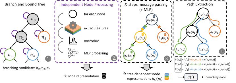
Figure 1: Our method: (1) SCIP solves individual nodes and executes existing heuristics. (2) Features are extracted from every branch-and-bound node and sent to individual normalization and embedding. (3) The node embeddings are subject to $K$ steps of GNN message passing on the induced tree-structure. (4) Based on the node embeddings, we generate root-to-leave paths, from which we sample the next node. The resulting node is submitted to SCIP and we return to step 1.

BnB is one of the most effective methods for solving mixed integer programming (MIP) problems. It recursively solves relaxed versions of the original problem, gradually strengthening the constraints until it finds an optimal solution. The first step relaxes the original MIP instance into a tractable subproblem by dropping all integrality constraints such that the subproblem can later be strictified into a MIP solution. For simplicity, we focus our explanation to the case of mixed integer linear programs (MILP) while our method theoretically works for any type of constraint allowed in SCIP (see nonlinear results in Sec. 5.3.2, and (Bestuzheva et al., 2023). Concretely a MILP has the form

$$P_{\text{MILP}}=\min\{c^{T}_{1}x+c^{T}_{2}y|Ax+By\geq b,y\in\mathbb{Z}^{n}\},$$ (1)

where $c_{1}$ and $c_{2}$ are coefficient vectors, $A$ and $B$ are constraint matrices, and $x$ and $y$ are variable vectors. The integrality constraint $y\in\mathbb{Z}^{n}$ requires $y$ to be an integer. In the relaxation step, this constraint is dropped, leading to the following simplified problem:

$$P_{\text{relaxed}}=\min\{c^{T}_{1}x+c^{T}_{2}y|Ax+By\geq b\}.$$ (2)

Now, the problem becomes a linear program without integrality constraints, which can be exactly solved using the Simplex (Dantzig, 1982) or other efficient linear programming algorithms.

After solving the relaxed problem, BnB proceeds to the branching step: First, a non-integral $y_{i}$ is chosen. The branching step then derives two problems: The first problem (Eq. 3) adds a lower bound to variable $y_{i}$, while the second problem (Eq. 4) adds an upper bound to variable $y_{i}$. These two directions represent the rounding choices to enforce integrality for $y_{i}$:

$$P_{\text{relaxed}}\cup\{y\leq c\} =\min\{c^{T}_{1}x+c^{T}_{2}y|Ax+By\geq b,y_{i}\leq\lfloor c\rfloor\}$$ (3)

$$P_{\text{relaxed}}\cup\{y\geq c+1\} =\min\{c^{T}_{1}x+c^{T}_{2}y|Ax+By\geq b,y_{i}\geq\lceil c\rceil\}$$ (4)

The resulting decision tree, with two nodes representing the derived problems can now be processed recursively. However, a naive recursive approach exhaustively enumerates all integral vertices, leading to an impractical computational effort. Hence, in the bounding step, nodes that are deemed worse than the currently known best solution are discarded. To do this, BnB stores previously found solutions which can be used as a lower bound to possible solutions. If a node has an upper bound larger than a currently found integral solution, no node in that subtree has to be processed.

The interplay of these three steps—relaxation, branching, and bounding—forms the core of branch-and-bound. It enables the systematic exploration of the solution space while efficiently pruning unpromising regions. Through this iterative process, the algorithm converges towards the optimal solution for the original MIP problem, while producing exact optimality bounds at every iteration.

The success of branch and bound hinges on the effective utilization of various heuristics throughout the optimization process. Primal heuristics, for instance, aim to directly find integral solutions from non-integral subproblems, whereas variable selection heuristics strive to identify high-value variables to branch on. All of these heuristics are of crucial importance for modern state-of-the-art solvers such as SCIP (Bestuzheva et al., 2021a; b), as finding better results allows for much more aggressive pruning of the search tree, which can speed up the problem exponentially.

There are many extensions to this method, such as the branch-and-cut algorithm (Padberg & Rinaldi, 1991) that extends the “derelaxation” procedure using cutting planes which are necessary to reach high performance, but at its core branch-and-bound algorithms are the workhorse behind state-of-the-art MILP, due to their high degree of generality, excellent pruning and strong numerical stability.

3 Related Work

While variable selection through learned heuristics has been studied a lot (see e.g. Parsonson et al. (2022) or Etheve et al. (2020)), learning node selection, where learned heuristics pick the best node to continue, have only rarely been addressed in research. We study learning algorithms for node selection in state-of-the-art branch-and-cut solvers. Prior work that learns such node selection strategies made significant contributions to improve the efficiency and effectiveness of the optimization.

Notably, many approaches rely on per-node features and IL. Otten & Dechter (2012) examined the estimation of subproblem complexity as a means to enhance parallelization efficiency. By estimating the complexity of subproblems, the algorithm can allocate computational resources more effectively. Yilmaz & Yorke-Smith (2021) employed IL to directly select the most promising node for exploration. Their approach utilized a set of per-node features to train a model that can accurately determine which node to choose. He et al. (2014) employed support vector machines and IL to create a hybrid heuristic based on existing heuristics. By leveraging per-node features, their approach aimed to improve node selection decisions. While these prior approaches have yielded valuable insights, they are inherently limited by their focus on per-node features.

Labassi et al. (2022) proposed the use of Siamese graph neural networks, representing each node as a graph that connects variables with the relevant constraints. Their objective was direct imitation of an optimal diving oracle. This approach facilitated learning from node comparisons and enabled the model to make informed decisions during node selection. However, the relative quality of two nodes cannot be fully utilized to make informed branching decisions as interactions between nodes remain minimal (as they are only communicated through a final score and a singular global embedding containing the primal and dual estimate). While the relative quality of nodes against each other is used, the potential performance is limited as the overall (non-leaf) tree structure is not considered.

Another limitation of existing methods is their heavy reliance on pure IL that will be constrained by the performance of the existing heuristics. Hence, integrating RL to strategically select nodes holds great promise. This not only aims for short-term optimality but also for the acquisition of valuable information to make better decisions later in the search process. This is important as node selection not only has to model the expected decrease in the optimality gap, but also has to account for the time commitment a certain node brings with it as not all nodes take equal amount of time to process.

4 Methodology

We combine two major objectives: a representation that effectively captures the inherent structures and complexities of the branch-and-bound tree, see Sec. 4.1, and an RL policy trained to select nodes (instead of an heuristic guided via RL), see Sec. 4.2. To do this, we view node-selection as a probabilistic process where different nodes $n_{k}$ can be sampled from a distribution $\pi$: $n_{k}\sim\pi(n_{k}|s_{o})$, where $s_{o}$ is the state of the branch-and-bound optimizer. Optimal node selection can now be framed as learning a node-selection distribution $\pi$ that, given some representation of the optimizer state $s_{o}$, selects the optimal node $n_{i}$ to maximize a performance measure. A reasonable performance measure, for instance, captures the achieved performance against a well-known baseline. In our case, we choose our performance measure, i.e., our reward, to be

$$r=-\left(\frac{\text{{gap(node selector)}}}{\text{{gap(scip)}}}-1\right)$$ (5)

The aim is to decrease the optimality gap achieved by our node-selector (i.e., gap(node selector)), normalized by the results achieved by the existing state-of-the-art node-selection methods in the SCIP (Bestuzheva et al., 2021a) solver (i.e., gap(scip)). We further shift this performance measure, such that any value $>0$ corresponds to our selector being superior to existing solvers, while a value $<0$ corresponds to our selector being worse, and clip the reward objective between $(1,-1)$ to ensure equal size of the reward and “punishment” ranges. In general, finding good performance measurements that are, for example, invariant to the overall problem difficulty, is difficult (see Sec. 5). For training we can circumvent a lot of the downsides of this reward formulation, like divide-by-zero or divide-by-infinity problems, by simply sampling difficult, but tractable problems (see Sec. 4.3).

4.1 Tree Representation

To address the first objective, we propose a novel approach that involves bi-simulating the existing branch-and-bound tree using a graph neural network (GNN). This entails transforming the tree into a graph structure, taking into account the features associated with each node (for a full list of features we used, see Appendix C). We ensure that the features stay at a constant size, independent from, e.g., the number of variables and constraints, to enable efficient batch-evaluation of the entire tree.

In the reconstructed GNN, the inputs consist of the features of the current node, as well as the features of its two child nodes. Pruned or missing nodes are replaced with a constant to maintain the integrity of the graph structure. This transformation enables us to consider subtrees within a predetermined depth limit, denoted as $K$, by running $K$ steps of message passing. This approach allows us to balance memory and computational requirements across different nodes, while preventing the overload of latent dimensions in deep trees.

For our graph processing GNN, we use a well understood method known as “Message Passing” across nodes. For all nodes, this method passes information from the graph’s neighborhood into the node itself, by first aggregating all information with a permutation invariant transform (e. g., computing the mean across neighbors), and then updating the node-state with the neighborhood state. In our case, the (directed) neighborhood is simply the set of direct children (see Fig. 1). As message passing iterates, we accumulate increasing amounts of the neighborhood, as iteration $t+1$ utilizes a node-embedding that already has the last $t$ steps aggregated. Inductively, the message passing range directly correlates with the number of iterations used to compute the embeddings.

Concretely, the internal representation can be thought of initializing $h_{0}(n)=x(n)$ (with $x(n)$ being the feature associated with node $n$) and then running $K$ iterations jointly for all nodes $n$:

$$h_{t+1}(n)=h_{t}(n)+\operatorname{emb}\left(\frac{h_{t}(\operatorname{left}(n))+h_{t}(\operatorname{right}(n))}{2}\right),$$ (6)

where $\operatorname{left}(n)$ and $\operatorname{right}(n)$ are the left and right children of $n$, respectively, $h_{t}(n)$ is the hidden representation of node $n$ after $t$ steps of message passing, and $\operatorname{emb}$ is a function that takes the mean hidden state of all embeddings and creates an updated node embedding.

4.2 RL for Node Selection

Using the final node-representation $h_{K}(n)$ we can now derive a value for every node $V(h_{K}(n))$ and a weight $W(h_{K}(n))$ to be used by our RL agent. Specifically we can produce a probability distribution of node-selections (i. e., our actions) by computing the expected weight across the unique path from the graph’s root to the “to-be-selected” leaves. We specifically consider the expectation as to not bias against deeper or shallower nodes. This definition allows us to have a global view on the node-selection probability, despite the fact that we only perform a fixed number of message-passing iterations to derive our node embeddings. Concretely, let $n$ be a leaf node in the set of candidate nodes $\mathscr{C}$, also let $P(r,n)$ be the unique path from the root $r$ to the candidate leaf node, with $|P(r,n)|$ describing its length. We define the expected path weight $W^{\prime}(n)$ to a leaf node $n\in\mathscr{C}$ as

$$W^{\prime}(n)=\frac{1}{|P(r,n)|}\sum_{u\in P(r,n)}W(h_{K}(u)).$$ (7)

Selection now is performed in accordance to sampling from a selection policy $\pi$ induced by

$$\pi(n|\operatorname{tree})=\operatorname{softmax}\left(\{W^{\prime}(n)|\forall n\in\mathscr{C}\right\}).$$ (8)

Intuitively, this means that we select a node exactly if the expected utility along its path is high. Note that this definition is naturally self-correcting as erroneous over-selection of one subtree will lead to that tree being completed, which removes the leaves from the selection pool $\mathscr{C}$.

By combining the bi-simulation technique, the GNN representation, and the computation of node probabilities, we establish a framework that enables distributional RL for node selection. We consider proximal policy optimization (PPO) (Schulman et al., 2017) for optimizing the node-selection policy. For its updates, PPO considers the advantage $A$ of the taken action in episode $i$ against the current action distribution. Intuitively, this amounts to reducing the frequency of disadvantageous actions, while increasing the frequency of high quality actions. We choose the generalized advantage estimator (GAE) (Schulman et al., 2015), which interpolates between an unbiased but high variance Monte Carlo estimator, and a biased, low variance estimator. For the latter we use a value function $V(s)$, which we implemented similarly to the policy-utility construction above:

$$Q(n|s) =\frac{\tilde{Q}(n|s)}{|P(r,n)|}$$ (9)

$$\tilde{Q}(n|s) =\tilde{Q}(\text{left child}|s)+\tilde{Q}(\text{right child}|s)+q(h_{n}|s)$$ (10)

$$V(s) =\left\{\max Q(n)\hskip 5.69054pt|\hskip 5.69054pt\forall n\in\mathscr{C}\right\}$$ (11)

where $q(h_{n})$ is the per-node estimator, $\tilde{Q}$ the unnormalized Q-value, and $\mathscr{C}$ is the set of open nodes as proposed by the branch-and-bound method. Note that this representation uses the fact that the value function can be written as the maximal $Q$-value: $V(s)=\max_{a\in A}Q(a|s)$.

This method provides low, but measurable overhead compared to existing node selectors, even if we discount the fact that our Python-based implementation is vastly slower than SCIP’s highly optimized C-based implementations. Hence, we focus our model on being efficient at the beginning of the selection process, where good node selections are exponentially more important as finding more optimal solutions earlier allows to prune more nodes from the exponentially expanding search tree. Specifically we evaluate our heuristic at every node for the first 250 selections, then at every tenth node for the next 750 nodes, and finally switch to classical selectors for the remaining nodes.

4.3 Data Generation & Agent Training

In training MIPs, a critical challenge lies in generating sufficiently complex training problems. First, to learn from interesting structures, we need to decide on some specific problem, whose e. g., satisfiability is knowable as generating random constraint matrices will likely generate empty polyhedrons, or polyhedrons with many eliminable constraints (e.g., in the constraint set consisting of $c^{T}x\leq b$ and $c^{T}x\leq b+\rho$ with $\rho\neq 0$ one constraint is always eliminable). This may seem unlikely, but notice how we can construct aligned $c$ vectors by linearly combining different rows (just like in LP-dual formulations). Deciding if such a polytope is empty itself is already NP-hard as elimination of constraints amounts to an implicit Fourier-Motzkin elimination (Motzkin, 1936) which runs in double-exponential time. In practice, selecting a sufficiently large class of problems may be enough as during the branch-and-cut process many sub-polyhedra are anyways being generated. Since our algorithm naturally decomposes the problem into sub-trees, we can assume any policy that performs well on the entire tree also performs well on sub-polyhedra generated during the branch-and-cut.

For this reason we consider the large class of Traveling Salesman Problem (TSP), which itself has rich use-cases in planning and logistics, but also in optimal control, the manufacturing of microchips and DNA sequencing (see Cook et al. (2011)). The TSP problem consists of finding a round-trip path in a weighted graph, such that every vertex is visited exactly once, and the total path-length is minimal (for more details and a mathematical formulation, see Appendix A)

For training, we would like to use random instances of TSP but generating them can be challenging. Random sampling of distance matrices often results in easy problem instances, which do not challenge the solver. Consequently, significant effort has been devoted to devising methods for generating random but hard instances, particularly for problems like the TSP, where specific generators for challenging problems have been designed (see Vercesi et al. (2023) and Rardin et al. (1993)).

However, for our specific use cases, these provably hard problems may not be very informative as they rarely contain efficiently selectable nodes. The inherent difficulty of these instances, reflected in the lack of, e.g., an efficient node-selection method, renders them less relevant for our purpose – this lack of a P-time selection method is what makes them hard in the first place. Assuming $P\neq NP$, it is unreasonable to expect our algorithm to tackle these provably hard instances effectively. Hence, we focus on hard but tractable problems. These problems strike a balance, providing challenges to our solver while remaining amenable to improvement through node selection.

To generate these intermediary-difficult problems, we adopt a multi-step approach: We begin by generating random instances and then apply some mutation techniques (Bossek et al., 2019) to introduce variations, and ensure diversity within the problem set. From this population of candidate problems, we select the median optimality-gap problem. The optimality gap, representing the best normalized difference between the lower and upper bound for a solution found during the solver’s budget-restricted execution, serves as a crucial metric to assess difficulty.

To ensure the quality of candidate problems, we exclude problems with more than $100\%$ or zero optimality gap, as these scenarios present challenges in reward assignment during RL. To reduce overall variance of our training, we limit the ground-truth variance in optimality gap. Additionally, we impose a constraint on the minimum number of nodes in the problems, discarding every instance with less than 100 nodes. This is essential as we do not expect such small problems to give clean reward signals to the reinforcement learner.

5 Experiments

For our experiments we consider the instances of TSPLIB (Reinelt, 1991) and MIPLIB (Gleixner et al., 2021) which are one of the most used datasets for benchmarking MIP frameworks and thusly form a strong baseline to test against. We further test against the UFLP instance generator by (Kochetov & Ivanenko, 2005), which specifically produces instances hard to solve for branch-and-bound, and against MINLPLIB (Bussieck et al., 2003), which contains mixed integer nonlinear programs, to show generalization towards very foreign problems.

One issue in benchmarking these instances is the general range of different problems in difficulty and scale of the different models. For instance, TSPLIB features problems ranging from a dozen to multiple thousand cities, with difficulties ranging from seconds of solver time to hours.

5.1 Baselines

We run both our method and SCIP for 45s. We then filter out all runs where SCIP has managed to explore less than 5 nodes, as in these runs we cannot expect even perfect node selection to make any difference in performance. If we included those in our average, we would have a significant number of lines where our node-selector has zero advantage over the traditional SCIP one, not because our selector is better or worse than SCIP, but simply because it wasn’t called in the first place. We set this time-limit relatively low as our prototype selector only runs at the beginning of the solver process, meaning that over time the effects of the traditional solver take over. Running the system for longer yields similar trends, but worse signal-to-noise ratio in the improvement due to the SCIP selector dominating the learnt solver in the long-runtime regime.

A common issue in testing new node selection techniques against an existing (e.g., SCIP) strategy is the degree of code-optimization present in industrial-grade solvers compared to research prototypes: SCIP is a highly optimized C-implementation while our node selector has Python and framework overhead to contend with. This means the node-throughput is naturally going to be much slower than the node-throughput of the baseline, even if we disregard the additional cost of evaluating the neural network. We cannot assess the theoretically possible efficiency of our method, so all of our results should be taken as a lower-bound on performance.

5.2 Evaluation Metrics

A core issue in benchmarking is the overall breadth of difficulty and scale of problem instances. Comparing the performance of node selection strategies is challenging due to a lack of aggregatable metrics. Further, the difficulty of the instances in benchmarks do not only depend on the scale but also specific configuration, e.g., distances in TSPLIB: while swiss42 can be solved quickly, ulysses22 cannot be solved within our time limit despite only being half the size (see Table 3). We can also see this at the range of optimality gaps in Table 3. The gaps range from $1134\%$ to $0\%$. Computing the mean gap alone is not very meaningful as instances with large gaps dominate the average. To facilitate meaningful comparisons, we consider three normalized metrics as follows.

The Reward (Eq. 5) considers the shifted ratio between the optimality gap of our approach and that of the baseline; positive values represent that our method is better and vice verse. This has the natural advantage of removing the absolute scale of the gaps and only considering relative improvements. The downside is that small differences can get blown-up in cases where the baseline is already small. Note that the function also has an asymmetric range, since one can have an infinitely negative reward, but can have at most have a $+1$ positive reward. Hence, we clip the reward in the range $\pm 1$ as this means a single bad result cannot destroy the entire valuation for either method.

Utility defines the difference between both methods normalized using the maximum of both gaps:

$$\operatorname{Utility}=\left(\frac{\text{{gap(scip)}}-\text{{gap(node selector)}}}{\max\left(\text{{gap(node selector)}},\text{{gap(scip)}}\right)}\right).$$ (12)

The reason we do not use this as a reward measure is because we empirically found it to produce worse models. This is presumably because some of the negative attributes of our reward, e.g., the asymmetry of the reward signal, lead to more robust policies. In addition, the utility metric gives erroneous measurements when both models hit zero optimality gap. This is because utility implicitly defines $\frac{0}{0}=0$, rather than reward, which defines it as $\frac{0}{0}=1$. In some sense the utility measurement is accurate, in that our method does not improve upon the baseline. On the other hand, our method is already provably optimal as soon as it reaches a gap of $0\%$. In general, utility compresses the differences more than reward which may or may not be beneficial in practice.

Utility per Node normalizes Utility by the number of nodes used during exploration:

$$\operatorname{Utility/Node}=\left(\frac{\operatorname{scip}-\operatorname{selector}}{\max\left(\operatorname{selector},\operatorname{scip}\right)}\right),$$ (13a)

where $\operatorname{selector}=\frac{\text{{gap(node selector)}}}{\text{{nodes(node selector)}}}$ and $\operatorname{scip}=\frac{\text{{gap(scip)}}}{\text{{nodes(scip)}}}$. The per-node utility gives a proxy for the total amount of “work” done by each method. However, it ignores the individual node costs, as solving the different LPs may take different amounts of resources (a model with higher “utility/node” is not necessarily more efficient as our learner might pick cheap but lower expected utility nodes on purpose). Further, the metric is underdefined: comparing two ratios, a method may become better by increasing the number of nodes processed, but keeping the achieved gap constant. In practice the number of nodes processed by our node selector is dominated by the implementation rather than the node choices, meaning we can assume it is invariant to changes in policy. Another downside arises if both methods reach zero optimality gap, the resulting efficiency will also be zero regardless of how many nodes we processed. As our method tend to reach optimality much faster (see Sec. 5 and Appendix D), all utility/node results can be seen as a lower-bound for the actual efficiency.

5.3 Results

While all results can be found in Appendix D we report an aggregated view for each benchmark in Table 1. In addition to our metrics we report the winning ratio of our method over the baseline.

Table 1: Performance across benchmarks (the policy only saw TSP instances during training).

Benchmark	Reward	Utility	Utility/Node	Percentage Winning
TSPLIB (Reinelt, 1991)	0.184	0.030	0.193	0.50
UFLP (Kochetov & Ivanenko, 2005)	0.078	0.093	-0.064	0.636
MINLPLib (Bussieck et al., 2003)	0.487	0.000	0.114	0.852
MIPLIB (Gleixner et al., 2021)	0.140	-0.013	0.208	0.769

For benchmarking and training, we leave all settings, such as presolvers, primal heuristics, diving heuristics, constraint specialisations, etc. at their default settings to allow the baseline to perform best. All instances get a budget of 45$\mathrm{s}$ and all instances are solved using the same model without any fine-tuning. We expect that tuning, e.g., the aggressiveness of primal heuristics, increases the performance of our method, as it decreases the relative cost of evaluating a neural network, but for the sake of comparison we use the same parameters. We train our node selection policy on problem instances according to Sec. 4.3 and apply it on problems from different benchmarks.

First, we will discuss TSPLIB itself, which while dramatically more complex than our selected training instances, still contains instances from the same problem family as the training set (Sec. 5.3.1). Second, we consider instances of the Uncapacitated Facility Location Problem (UFLP) as generated by Kochetov & Ivanenko (2005)’s problem generator. These problems are designed to be particulary challenging to branch-and-bound solvers due to their large optimality gap (Sec. D.3.1). While the first two benchmarks focused on specific problems (giving you a notion of how well the algorithm does on the problem itself) we next consider “‘meta-benchmarks” that consist of many different problems, but relatively few instances of each. MINLPLIB (Bussieck et al., 2003) is a meta-benchmark for nonlinear mixed-integer programming (Sec. 5.3.2), and MIPLIB (Gleixner et al., 2021) a benchmark for mixed integer programming (Sec. 5.3.3). We also consider generalisation against the uncapacitated facility location problem using a strong instance generator, see Appendix D.3.1. Our benchmarks are diverse and complex and allow to compare algorithmic improvements in state-of-the-art solvers.

5.3.1 TSPLIB

From an aggregative viewpoint we outperform the SCIP node selection by $\approx 20\%$ in both reward and utility per node. Due to the scoring of zero-gap instances we are only $3.3\%$ ahead in utility. If both our method and the baseline reach an optimality gap of $0$, it is unclear how the normalised reward should appear. “Reward” defines $\frac{0}{0}=1$ as our method achieved the mathematically optimal value, so it should achieve the optimal reward. “Utility” defines $\frac{0}{0}=0$ as our method did not improve upon the baseline. While this also persists in “utility per node”, our method is much more efficient compared to the baseline s.t. zero-gap problems do not affect our results much.

Qualitatively, it is particularly interesting to study the problems our method still looses against SCIP (in four cases). A possible reason why our method significantly underperforms on Dantzig42 is that our implementation is just too slow, considering that the baseline manages to evaluate $\approx 40\%$ more nodes. A similar observation can be made on eil51 where the baseline manages to complete $5\times$ more nodes. KroE100 is the first instance our method looses against SCIP, although it explores an equal amount of nodes. We believe that this is because our method commits to the wrong subtree early and never manages to correct into the proper subtree. rd100 is also similar to Dantzig and eil51 as the baseline is able to explore $60\%$ more nodes. Ignoring these four failure cases, our method is either on par (up to stochasticity of the algorithm) or exceeds the baseline significantly.

It is also worthwhile to study the cases where both the baseline and our method hit $0$ optimality gap. A quick glance at instances like bayg29, fri26, swiss42 or ulysses16 shows that our method tends to finish these problems with significantly fewer nodes explored. This is not captured by any of our metrics as the “utility/node” metric is zero if the utility is zero, as is the case with $0$ optimality gap instances. Qualitatively, instances like bayg29 manage to reach the optimum in only $\frac{1}{3}$ the number of explored nodes, which showcases a significant improvement in node-selection quality. It is worth noting that, due to the different optimization costs for different nodes, it not always holds that evaluating fewer nodes is faster in wall-clock time. In practice, “fewer nodes is better” seems to be a good rule-of-thumb to check algorithmic efficiency.

5.3.2 MINLPLIB

We now consider MINLPs. To solve these, SCIP and other solvers use branching techniques that cut nonlinear (often convex) problems from a relaxed master-relaxation towards true solutions. We consider MINLPLib (Bussieck et al., 2003), a meta-benchmark consisting of hundreds of synthetic and real-world MINLP instances of varying different types and sizes. As some instances take hours to solve (making them inadequate to judge our node selector which mainly aims to improve the starting condition of problems), we also pre-filter the instances. Specifically, we apply the same filtering for tractable problems as in the TSPLIB case. Full results can be found in Appendix D.3.

Our method still manages to outperform SCIP, even on MINLPs, although it has never seen a single MINLP problem before, see Table 1. The reason for the significant divergence between the Reward and Utility performance measures is once again due to the handling of $\frac{0}{0}$. Since MINLPLIB contains a fair few “easy” problems that can be solved to $0\%$ gap, this has a much bigger effect on this benchmark than the others. Qualitatively, our method either outperforms or is on par with the majority of problems, but also loses significantly in some problems, greatly decreasing the average. Despite the fact that utility “rounds down” advantages to zero, the overall utility per node is still significantly better than that of SCIP. Inspecting the instances with poor results, we also see that for most of them the baseline manages to complete significantly more nodes than our underoptimized implementation. We expect features specifically tuned for nonlinear problems to increase performance by additional percentage points, but as feature selection is orthogonal to the actual algorithm design, we leave more thorough discussion of this to future work .

5.3.3 MIPLIB

Last, but not least we consider the meta-benchmark MIPLIB (Gleixner et al., 2021), which consists of hundreds of real-world mixed-integer programming problems of varying size, complexity, and hardness. Our method is either close to or exceeds the performance of SCIP, see Table 1. It is also the first benchmark our method looses on, according to the utility-metric.

Considering per-instance results, we see similar patterns as in previous failure cases: Often we underperform on instances that need to close many nodes, as our method’s throughput lacks behind that of SCIP. We expect that a more efficient implementation alleviates the issues in those cases.

We also see challenges in problems that are far from the training distribution. Consider fhnw-binpack4-48, were the baseline yields an optimality gap of $0$ while we end at $+\infty$. This is due to the design of the problem: Instead of a classical optimization problem, this is a satisfaction problem, where not an optimal value, but any valid value is searched, i.e., we either yield a gap of $0$, or a gap of $+\infty$, as no other gap is possible. Notably, these kinds of problems may pose a challenge for our algorithm, as the node-pruning dynamics of satisfying MIPs are different than the one for optimizing MIPs: Satisfying MIPs can only rarely prune nodes since, by definition, no intermediary primally valid solutions are ever found. We believe this problem could be solved by considering such problems during training, which we currently do not.

6 Conclusion

We have proposed a novel approach to branch-and-bound node selection, leveraging the power of bisimulation and RL. By aligning our model with the branch-and-bound tree structure, we have demonstrated the potential to develop a versatile heuristic that can be applied across various optimization problem domains, despite being trained on a narrow set of instances. To our knowledge, this is the first demonstration of learned node selection to mixed-integer (nonlinear) programming.

There are still open questions. Feature selection remains an area where we expect significant improvements, especially for nonlinear programming, which contemporary methods do not account for. We also expect significant improvements in performance through code optimization. An important area for research lies in generalized instance generation: Instead of focusing on single domain instances for training (e.g. from TSP), an instance generator should create problem instances with consistent, but varying levels of difficulty across different problem domains.

Appendix A TSP-as-MILP Formulation

In general, due to the fact that TSP is amongst the most studied problems in discrete optimization, we can expect existing mixed-integer programming systems to have rich heuristics that provide a strong baseline for our method. Mathematically, we choose the Miller–Tucker–Zemlin (MTZ) formulation (Miller et al., 1960):

$$\!\min_{x} \sum^{n}_{i=1}\sum^{n}_{j\neq i,j=1}c_{ij}x_{ij}$$ (14a)

subject to $$\sum^{n}_{j=1,i\neq j}x_{ij}=1 \forall i=1,\dots,n$$ (14b)

$$\sum^{n}_{i=1,i\neq j}x_{ij}=1 \forall j=1,\dots,n$$ (14c)

$$u_{1}-u_{j}+(n-1)x_{ij}\leq n-2 2\leq i\neq j\leq n$$ (14d)

$$2\leq u_{i}\leq n 2\leq i\leq n$$ (14e)

$$u_{i}\in\mathbb{Z},x_{ij}\in\{0,1\}$$ (14f)

Effectively this formulation keeps two buffers: one being the actual $(i,j)$-edges travelled $x_{ij}$, the other being a node-order variable $u_{i}$ that makes sure that $u_{i}<u_{j}$ if $i$ is visited before $j$. There are alternative formulations, such as the Dantzig–Fulkerson–Johnson (DFJ) formulation, which are used in modern purpose-built TSP solvers, but those are less useful for general problem generation: The MTZ formulation essentially relaxes the edge-assignments and order constraints, which then are branch-and-bounded into hard assignments during the solving process. This is different to DFJ, which instead relaxes the “has to pass through all nodes” constraint. DFJ allows for subtours (e. g., only contain node $A,B,C$ but not $D,E$) which then get slowly eliminated via the on-the-fly generation of additional constraints. To generate these constraints one needs specialised row-generators which, while very powerful from an optimization point-of-view, make the algorithm less general as a custom row-generator has to intervene into every single node. However, in our usecase we also do not really care about the ultimate performance of individual algorithms as the reinforcement learner only looks for improvements to the existing node selections. This means that as long as the degree of improvement can be adequately judged, we do not need state-of-the-art solver implementations to give the learner a meaningful improvement signal.

Appendix B Uncapacitated facility location Problem

Mathmatically, the uncapacitated facility location problem can be seen as sending a product $z_{ij}$ from facility $i$ to consumer $j$ with cost $c_{ij}$ and demand $d_{j}$. One can only send from $i$ to $j$ if facility $i$ was built in the first place, which incurs cost $f_{i}$. The overall problem therefore is

$$\!\min_{x} \sum^{n}_{i=1}\sum^{m}_{i=1}c_{ij}d_{j}z_{ij}+\sum^{n}_{i=0}f_{i}x_{i}$$ (15a)

subject to $$\sum^{n}_{j=1,i\neq j}z_{ij}=1 \forall i=1,\dots,m$$ (15b)

$$\sum^{n}_{i=1,i\neq j}z_{ij}\leq Mx_{i} \forall j=1,\dots,n$$ (15c)

$$z_{ij}\in\{0,1\} \forall i=1,\dots,n,\forall j=1,\dots,m$$ (15d)

$$x_{i}\in\{0,1\} \forall i=1,\dots,n$$ (15e)

where $M$ is a suitably large constant representing the infinite-capacity one has when constructing $x_{i}=1$. One can always choose $M\geq m$ since that, for the purposes of the polytop is equivalent to setting $M$ to literal infinity. This is also sometimes referred to as the “big $M$” method.

The instance generator by Kochetov & Ivanenko (2005) works by setting $n=m=100$ and setting all opening costs at $3000$. Every city has 10 “cheap” connections sampled from $\{0,1,2,3,4\}$ and the rest have cost $3000$, which represents infinity (i. e., also invoking the big $M$ method).

Appendix C Features

Table 2 lists the features used on every individual node. The features split into two different types: One being “model” features, the other being “node” features. Model features describe the state of the entire model at the currently explored node, while node features are specific to the yet-to-be-solved added node. We aim to normalize all features with respect to problem size, as e. g., just giving the lower-bound to a problem is prone to numerical domain shifts. For instance a problem with objective $c^{T}x,x\in P$ is inherently the same from a solver point-of-view as a problem $10c^{T}x,x\in P$, but would give different lower-bounds. Since NNs are generally nonlinear estimators, we need to make sure such changes do not induce huge distribution shifts. We also clamp the feature values between $[-10,10]$ which represent “infinite” values, which can occur, for example in the optimality gap. Last but not least, we standardize features using empirical mean and standard deviation.

Table 2: Features used per individual node.

model features	Number of cuts applied	normalized by total number of constraints
	Number of separation rounds
	optimality gap
	lp iterations
	mean integrality gap
	percentage of variables already integral
	histogram of fractional part of variables	10 evenly sized buckets
node features
	depth of node	normalized by total number of nodes
	node lowerbound	normalized by min of primal and dual bound
	node estimate	normalized by min of primal and dual bound

These features are inspired by prior work, such as Labassi et al. (2022); Yilmaz & Yorke-Smith (2021), but adapted to the fact that we do not need e. g., explicit entries for the left or right child’s optimality gap, as these (and more general K-step versions of these) can be handled by the GNN.

Further, to make batching tractable, we aim to have constant size features. This is different from e. g., Labassi et al. (2022), who utilize flexibly sized graphs to represent each node. The upside of this approach is that certain connections between variables and constraints may become more apparent, with the downside being the increased complexity of batching these structures and large amounts of nodes used. This isn’t a problem for them, as they only consider pairwise comparisons between nodes, rather than the entire branch-and-bound graph, but for us would induce a great deal of complexity and computational overhead, especially in the larger instances. For this reason, we represent flexibly sized inputs, such as the values of variables, as histograms: i.e., instead of having $k$ nodes for $k$ variables and wiring them together, we produce once distribution of variable values with 10-buckets, and feed this into the network. This looses a bit of detail in the representation, but allows us to scale to much larger instances than ordinarily possible.

In general, these features are not optimized, and we would expect significant improvements from more well-tuned features. Extracting generally meaningful features from branch-and-bound is a nontrivial task and is left as a task for future work.

Appendix D Full Results

The following two sections contain the per-instance results on the two “named” benchmarks TSPLIB (Reinelt, 1991) and MINLPLIB (Bussieck et al., 2003). We test against the strong SCIP 8.0.4 baseline. Due to compatibility issues, we decided not to test against (Labassi et al., 2022) or (He et al., 2014): These methods were trained against older versions of SCIP, which not only made running them challenging, but also would not give valid comparisons as we cannot properly account for changes between SCIP versions. Labassi et al. (2022) specifically relies on changes to the SCIP interface, which makes porting to SCIP 8.0.4 intractable. In general, this shouldn’t matter too much, as SCIP is still demonstrably the state-of-the-art non-commercial mixed-integer solver, which frequently outperforms even closed-source commercial solvers (see Mittelmann (2021) for thorough benchmarks against other solvers), meaning outperforming SCIP can be seen as outperforming the state-of-the-art.

D.1 TSPLIB results

Table 3: Results on TSPLIB (Reinelt, 1991) after 45s runtime. Note that we filter out problems in which less than 5 nodes were explored as those problems cannot gain meaningful advantages even with perfect node selection. “Name” refers to the instances name, “Gap Base/Ours” corresponds to the optimization gap achieved by the baseline and our method respectively (lower is better), “Nodes Base/Ours” to the number of explored Nodes by each method, and “Reward”, “Utility” and “Utility Node” to the different performance measures as described in Section 5.

Name	Gap Ours	Gap Base	Nodes Ours	Nodes Base	Reward	Utility	Utility/Node
att48	0.287	0.286	1086	2670	-0.002	-0.002	0.593
bayg29	0.000	0.000	2317	7201	1.000	0.000	0.000
bays29	0.000	0.036	11351	10150	1.000	1.000	0.997
berlin52	0.000	0.000	777	1634	1.000	0.000	0.000
bier127	2.795	2.777	23	25	-0.007	-0.007	0.074
brazil58	0.328	0.644	1432	2182	0.491	0.491	0.666
burma14	0.000	0.000	96	65	1.000	0.000	0.000
ch130	8.801	8.783	48	43	-0.002	-0.002	-0.106
ch150	7.803	7.802	18	18	-0.000	-0.000	-0.000
d198	0.582	0.582	10	11	-0.000	-0.000	0.091
dantzig42	0.185	0.100	2498	3469	-0.847	-0.459	-0.248
eil101	2.434	2.430	31	61	-0.002	-0.002	0.491
eil51	0.178	0.017	828	4306	-1.000	-0.907	-0.514
eil76	0.432	1.099	309	709	0.607	0.607	0.829
fri26	0.000	0.000	1470	6721	1.000	0.000	0.000
gr120	7.078	7.083	41	43	0.001	0.001	0.047
gr137	0.606	0.603	30	25	-0.006	-0.006	-0.171
gr17	0.000	0.000	92	123	1.000	0.000	0.000
gr24	0.000	0.000	110	207	1.000	0.000	0.000
gr48	0.192	0.340	586	2479	0.435	0.435	0.866
gr96	0.569	0.552	93	182	-0.032	-0.031	0.472
hk48	0.071	0.106	2571	2990	0.324	0.324	0.419
kroA100	8.937	8.945	102	233	0.001	0.001	0.563
kroA150	11.343	11.340	23	21	-0.000	-0.000	-0.087
kroA200	13.726	13.723	5	7	-0.000	-0.000	0.286
kroB100	7.164	7.082	83	109	-0.011	-0.011	0.230
kroB150	10.965	10.965	16	14	0.000	0.000	-0.125
kroB200	11.740	11.740	7	6	0.000	0.000	-0.143
kroC100	8.721	8.754	118	133	0.004	0.004	0.116
kroD100	7.959	7.938	70	111	-0.003	-0.003	0.368
kroE100	8.573	2.952	105	108	-1.000	-0.656	-0.646
lin105	2.005	2.003	98	149	-0.001	-0.001	0.341
pr107	1.367	1.336	128	217	-0.024	-0.023	0.396
pr124	0.937	0.935	64	61	-0.001	-0.001	-0.048
pr136	2.351	2.350	31	45	-0.000	-0.000	0.311
pr144	2.228	2.200	47	37	-0.012	-0.012	-0.222
pr152	2.688	2.683	14	41	-0.002	-0.002	0.658
pr226	1.091	1.092	6	6	0.001	0.001	0.001
pr76	0.534	0.476	201	855	-0.123	-0.109	0.736
rat99	0.853	0.849	41	80	-0.005	-0.005	0.485
rd100	5.948	4.462	100	166	-0.333	-0.250	0.197
si175	0.270	0.270	8	7	0.000	0.000	-0.125
st70	0.586	3.018	379	1068	0.806	0.806	0.931
swiss42	0.000	0.000	1075	1133	1.000	0.000	0.000
ulysses16	0.000	0.000	18322	19553	1.000	0.000	0.000
ulysses22	0.103	0.127	13911	13313	0.191	0.191	0.154
Mean	NaN	NaN	1321	1799	0.184	0.030	0.193

D.2 MIPLIB results

Table 4: Results on MIPLIB (Gleixner et al., 2021) after 45s runtime. Note that we filter out problems in which less than 5 nodes were explored as those problems cannot gain meaningful advantages even with perfect node selection. “Name” refers to the instances name, “Gap Base/Ours” corresponds to the optimization gap achieved by the baseline and our method respectively (lower is better), “Nodes Base/Ours” to the number of explored Nodes by each method, and “Reward”, “Utility” and “Utility Node” to the different performance measures as described in Section 5. Note that all results where achieved with a policy only trained on TSP instances

Name	Gap Ours	Gap Base	Nodes Ours	Nodes Base	Reward	Utility	Utility/Node
30n20b8	2.662	$\infty$	147	301	1.000	1.000	1.000
50v-10	0.101	0.113	303	1094	0.103	0.103	0.752
CMS750_4	0.100	0.072	68	281	-0.389	-0.280	0.664
air05	0.000	0.000	248	523	1.000	0.000	0.000
assign1-5-8	0.085	0.087	17466	23589	0.030	0.030	0.282
binkar10_1	0.000	0.000	2843	2270	1.000	0.000	0.000
blp-ic98	0.127	0.127	26	43	0.001	0.001	0.396
bnatt400	$\infty$	$\infty$	547	1568	0.000	0.000	0.651
bnatt500	$\infty$	$\infty$	148	936	0.000	0.000	0.842
bppc4-08	0.038	0.038	1318	3277	0.000	0.000	0.598
cost266-UUE	0.130	0.143	468	770	0.094	0.094	0.449
csched007	$\infty$	$\infty$	558	1770	0.000	0.000	0.685
csched008	0.070	$\infty$	910	1179	1.000	1.000	1.000
cvs16r128-89	0.560	0.601	6	7	0.068	0.068	0.202
drayage-25-23	0.000	0.000	105	267	1.000	0.000	0.000
dws008-01	$\infty$	$\infty$	123	173	0.000	0.000	0.289
eil33-2	0.194	0.189	191	171	-0.025	-0.024	-0.127
fast0507	0.027	0.027	11	7	-0.003	-0.003	-0.366
fastxgemm-n2r6s0t2	18.519	18.519	785	2531	0.000	0.000	0.690
fhnw-binpack4-4	$\infty$	$\infty$	140002	152608	0.000	0.000	0.083
fhnw-binpack4-48	$\infty$	0.000	15019	24649	-1.000	-1.000	-1.000
fiball	0.029	0.036	442	610	0.200	0.200	0.420
gen-ip002	0.008	0.010	88794	125319	0.197	0.197	0.397
gen-ip054	0.008	0.010	157950	179874	0.207	0.207	0.263
glass-sc	0.580	0.495	200	328	-0.173	-0.148	0.285
glass4	1.123	1.033	37424	35671	-0.087	-0.080	-0.123
gmu-35-40	0.001	0.001	28534	27077	0.402	0.398	0.276
gmu-35-50	0.001	0.001	16456	22333	0.177	0.176	0.346
graph20-20-1rand	0.000	0.000	416	283	1.000	0.000	0.000
graphdraw-domain	0.421	0.430	49640	56798	0.022	0.022	0.145
ic97_potential	0.023	0.040	39316	30633	0.415	0.415	0.247
icir97_tension	0.011	0.006	6697	7943	-0.882	-0.468	-0.367
irp	0.000	0.000	6	6	1.000	0.000	0.000
istanbul-no-cutoff	0.514	0.393	37	28	-0.309	-0.236	-0.422
lectsched-5-obj	$\infty$	2.200	1192	1118	-1.000	-1.000	-1.000
leo1	0.118	0.113	34	108	-0.049	-0.046	0.670
leo2	0.345	0.135	49	61	-1.000	-0.609	-0.514
mad	$\infty$	$\infty$	78783	81277	0.000	0.000	0.031
markshare2	$\infty$	$\infty$	91135	127265	0.000	0.000	0.284
markshare_4_0	$\infty$	$\infty$	570277	682069	0.000	0.000	0.164
mas74	0.079	0.084	32005	26180	0.060	0.060	-0.129
mas76	0.014	0.015	49987	52401	0.060	0.060	0.100
mc11	0.008	0.009	333	1989	0.139	0.138	0.855
mcsched	0.090	0.086	439	1526	-0.049	-0.046	0.698
mik-250-20-75-4	0.000	0.000	10067	10120	1.000	0.000	0.000
milo-v12-6-r2-40-1	0.038	0.031	340	514	-0.242	-0.195	0.179
momentum1	2.868	2.868	10	9	-0.000	-0.000	-0.100
n2seq36q	0.665	0.665	5	6	0.000	0.000	0.167
n5-3	0.046	0.000	427	595	-1.000	-1.000	-1.000
neos-1171737	0.032	0.032	7	13	0.000	0.000	0.462
neos-1445765	0.000	0.000	190	263	1.000	0.000	0.000
neos-1456979	$\infty$	0.344	204	405	-1.000	-1.000	-1.000
neos-1582420	0.016	0.016	11	11	0.000	0.000	0.000
neos-2657525-crna	$\infty$	$\infty$	42826	45188	0.000	0.000	0.052
neos-2978193-inde	0.013	0.013	964	2178	0.000	0.000	0.557
neos-3004026-krka	$\infty$	$\infty$	1134	1163	0.000	0.000	0.025
neos-3024952-loue	$\infty$	$\infty$	246	377	0.000	0.000	0.347
neos-3046615-murg	2.515	2.631	66921	79117	0.044	0.044	0.191
neos-3083819-nubu	0.000	0.000	1683	1687	1.000	0.000	0.000
neos-3381206-awhea	0.000	0.000	969	230	1.000	0.000	0.000
neos-3402294-bobin	$\infty$	$\infty$	10	24	0.000	0.000	0.583
neos-3627168-kasai	0.003	0.008	6269	3338	0.577	0.577	0.205
neos-3754480-nidda	$\infty$	$\infty$	87703	106632	0.000	0.000	0.178
neos-4338804-snowy	0.024	0.028	37447	36741	0.125	0.125	0.107
neos-4387871-tavua	0.631	0.634	5	7	0.005	0.005	0.289
neos-4738912-atrato	0.016	0.006	529	1064	-1.000	-0.634	-0.265
neos-4954672-berkel	0.265	0.254	454	775	-0.043	-0.041	0.389
neos-5093327-huahum	0.539	0.559	5	6	0.036	0.036	0.197
neos-5107597-kakapo	2.639	5.077	1885	2332	0.480	0.480	0.580
neos-5188808-nattai	$\infty$	$\infty$	16	105	0.000	0.000	0.848
neos-5195221-niemur	106.417	106.417	11	12	0.000	0.000	0.083
neos-911970	0.000	0.000	3905	15109	1.000	0.000	0.000
neos17	0.000	0.000	2151	3346	1.000	0.000	0.000
neos5	0.062	0.059	66231	91449	-0.053	-0.050	0.235
neos859080	0.000	0.000	990	1227	1.000	0.000	0.000
net12	2.592	2.114	56	29	-0.227	-0.185	-0.578
ns1208400	$\infty$	$\infty$	82	150	0.000	0.000	0.453
ns1830653	2.831	1.242	334	686	-1.000	-0.561	-0.099
ns1952667	$\infty$	$\infty$	100	52	0.000	0.000	-0.480
nu25-pr12	0.000	0.000	119	153	1.000	0.000	0.000
nursesched-sprint02	0.000	0.000	9	7	1.000	0.000	0.000
nw04	0.000	0.000	6	6	1.000	0.000	0.000
pg	0.000	0.000	460	491	1.000	0.000	0.000
pg5_34	0.004	0.004	275	592	-0.023	-0.022	0.524
piperout-08	0.000	0.000	223	309	1.000	0.000	0.000
piperout-27	0.000	0.000	47	28	1.000	0.000	0.000
pk1	1.244	1.117	102268	120685	-0.113	-0.102	0.057
radiationm18-12-05	0.057	0.167	886	2569	0.661	0.661	0.883
rail507	0.033	0.033	10	9	0.000	0.000	-0.100
ran14x18-disj-8	0.115	0.092	458	975	-0.251	-0.200	0.412
rd-rplusc-21	$\infty$	$\infty$	137	3542	0.000	0.000	0.961
reblock115	0.106	0.139	80	731	0.238	0.238	0.917
rmatr100-p10	0.216	0.326	43	74	0.337	0.337	0.615
rocI-4-11	0.671	0.837	12054	7909	0.198	0.198	-0.181
rocII-5-11	3.479	1.568	164	287	-1.000	-0.549	-0.211
rococoB10-011000	1.244	1.258	12	26	0.012	0.012	0.544
rococoC10-001000	0.337	0.153	135	866	-1.000	-0.546	0.656
roll3000	0.000	0.000	1156	2046	1.000	0.000	0.000
sct2	0.001	0.002	2117	1215	0.619	0.615	0.332
seymour	0.044	0.035	176	563	-0.243	-0.195	0.611
seymour1	0.003	0.003	329	885	0.146	0.145	0.682
sp150x300d	0.000	0.000	148	124	1.000	0.000	0.000
supportcase18	0.081	0.081	178	1372	0.000	-0.000	0.870
supportcase26	0.224	0.231	11191	20287	0.031	0.031	0.465
supportcase33	27.788	0.371	15	28	-1.000	-0.987	-0.975
supportcase40	0.086	0.094	50	111	0.087	0.087	0.589
supportcase42	0.033	0.050	76	256	0.340	0.340	0.804
swath1	0.000	0.000	311	372	1.000	0.000	0.000
swath3	0.110	0.113	1442	2800	0.020	0.020	0.495
timtab1	0.126	0.094	22112	25367	-0.333	-0.250	-0.139
tr12-30	0.002	0.002	8941	14896	0.019	0.019	0.394
traininstance2	$\infty$	$\infty$	412	821	0.000	0.000	0.498
traininstance6	29.355	$\infty$	2549	6376	1.000	1.000	1.000
trento1	3.885	3.885	4	7	-0.000	-0.000	0.429
uct-subprob	0.249	0.195	225	263	-0.276	-0.216	-0.084
var-smallemery-m6j6	0.062	0.062	95	224	-0.002	-0.002	0.575
wachplan	0.125	0.125	422	712	0.000	0.000	0.407
Mean	—	—	16538	19673	0.140	-0.013	0.208

D.3 MINLPLIB results

Table 5: Results on MINLPLIB (Bussieck et al., 2003) after 45s runtime. Note that we filter out problems in which less than 5 nodes were explored as those problems cannot gain meaningful advantages even with perfect node selection. “Name” refers to the instances name, “Gap Base/Ours” corresponds to the optimization gap achieved by the baseline and our method respectively (lower is better), “Nodes Base/Ours” to the number of explored Nodes by each method, and “Reward”, “Utility” and “Utility Node” to the different performance measures as described in Section 5. For all three measures, higher is better.

Name	Gap Ours	Gap Base	Nodes Ours	Nodes Base	Reward	Utility	Utility/Node
ball_mk4_05	0.000	0.000	1819	1869	1.000	0.000	0.000
ball_mk4_10	$\infty$	$\infty$	31684	37656	0.000	0.000	0.159
ball_mk4_15	$\infty$	$\infty$	1773	2415	0.000	0.000	0.266
bayes2_20	$\infty$	$\infty$	3171	2719	0.000	0.000	-0.143
bayes2_30	$\infty$	$\infty$	4462	4992	0.000	0.000	0.106
bayes2_50	$\infty$	$\infty$	2934	2530	0.000	0.000	-0.138
blend029	0.000	0.000	812	804	1.000	0.000	0.000
blend146	0.097	0.105	12390	18066	0.075	0.075	0.365
blend480	0.071	0.000	4878	6312	-1.000	-1.000	-0.999
blend531	0.000	0.000	3150	7161	1.000	0.000	0.000
blend718	0.898	0.796	22652	26060	-0.127	-0.113	0.020
blend721	0.000	0.000	4650	2708	1.000	0.000	0.000
blend852	0.021	0.000	7726	5413	-1.000	-1.000	-0.997
camshape100	0.076	0.074	18839	22205	-0.027	-0.026	0.128
camshape200	0.145	0.147	8199	9921	0.012	0.012	0.183
camshape400	0.198	0.195	4324	5275	-0.016	-0.016	0.167
camshape800	0.222	0.226	1504	1627	0.019	0.019	0.093
cardqp_inlp	1.436	1.660	4316	7232	0.135	0.135	0.484
cardqp_iqp	1.089	1.660	4766	7285	0.344	0.344	0.571
carton7	0.000	0.000	55	73	1.000	0.000	0.000
carton9	0.000	0.000	9848	7406	1.000	0.000	0.000
catmix100	$\infty$	$\infty$	186	8750	0.000	0.000	0.979
catmix200	$\infty$	$\infty$	123	3870	0.000	0.000	0.968
catmix400	$\infty$	$\infty$	146	3498	0.000	0.000	0.958
catmix800	$\infty$	$\infty$	75	333	0.000	0.000	0.775
celar6-sub0	$\infty$	$\infty$	4	6	0.000	0.000	0.333
chimera_k64ising-01	0.701	16.469	18	21	0.957	0.957	0.964
chimera_k64maxcut-01	0.523	0.199	57	198	-1.000	-0.618	0.246
chimera_k64maxcut-02	0.368	0.239	72	381	-0.536	-0.349	0.710
chimera_lga-02	0.893	0.893	5	6	0.000	0.000	0.167
chimera_mgw-c8-439-onc8-001	0.045	0.021	127	521	-1.000	-0.529	0.482
chimera_mgw-c8-439-onc8-002	0.067	0.046	72	526	-0.449	-0.310	0.802
chimera_mgw-c8-507-onc8-01	0.232	0.233	26	99	0.003	0.003	0.738
chimera_mgw-c8-507-onc8-02	0.188	0.346	14	25	0.455	0.455	0.695
chimera_mis-01	0.000	0.000	7	7	1.000	0.000	0.000
chimera_mis-02	0.000	0.000	7	7	1.000	0.000	0.000
chimera_rfr-01	1.029	1.153	70	61	0.108	0.108	-0.023
chimera_rfr-02	1.148	1.061	74	63	-0.082	-0.076	-0.213
chimera_selby-c8-onc8-01	0.436	0.224	34	111	-0.941	-0.485	0.406
chimera_selby-c8-onc8-02	0.439	0.232	40	92	-0.895	-0.472	0.176
clay0203m	0.000	0.000	19	30	1.000	0.000	0.000
clay0204m	0.000	0.000	266	400	1.000	0.000	0.000
clay0205m	0.000	0.000	4058	3908	1.000	0.000	0.000
clay0303m	0.000	0.000	107	45	1.000	0.000	0.000
clay0304m	0.000	0.000	337	897	1.000	0.000	0.000
clay0305m	0.000	0.000	4057	4204	1.000	0.000	0.000
color_lab3_3x0	1.445	1.725	320	576	0.162	0.162	0.534
color_lab3_4x0	5.581	5.455	265	434	-0.023	-0.023	0.375
crossdock_15x7	4.457	8.216	654	1080	0.458	0.458	0.672
crossdock_15x8	8.578	84.148	391	717	0.898	0.898	0.944
crudeoil_lee1_06	0.000	0.000	48	57	1.000	0.000	0.000
crudeoil_lee1_07	0.000	0.000	57	92	1.000	0.000	0.000
crudeoil_lee1_08	0.000	0.000	161	121	1.000	0.000	0.000
crudeoil_lee1_09	0.000	0.000	107	99	1.000	0.000	0.000
crudeoil_lee1_10	0.000	0.000	78	109	1.000	0.000	0.000
crudeoil_lee2_05	0.000	0.000	10	11	1.000	0.000	0.000
crudeoil_lee2_06	0.000	0.000	45	109	1.000	0.000	0.000
crudeoil_lee2_07	0.000	0.000	286	81	1.000	0.000	0.000
crudeoil_lee2_08	0.000	0.000	150	308	1.000	0.000	0.000
crudeoil_lee2_09	0.142	0.015	44	41	-1.000	-0.897	-0.904
crudeoil_lee3_05	0.000	0.000	1435	1820	1.000	0.000	0.000
crudeoil_lee3_06	0.057	0.013	352	1349	-1.000	-0.764	-0.095
crudeoil_lee4_05	0.000	0.000	306	118	1.000	0.000	0.000
crudeoil_lee4_06	0.000	0.000	129	60	1.000	0.000	0.000
crudeoil_lee4_07	0.000	0.000	193	89	1.000	0.000	0.000
crudeoil_lee4_08	0.000	0.001	41	53	0.187	0.184	0.371
crudeoil_li01	0.049	0.017	16819	11797	-1.000	-0.657	-0.758
crudeoil_li02	0.013	0.013	12172	10426	-0.027	-0.027	-0.165
crudeoil_li03	$\infty$	$\infty$	198	899	0.000	0.000	0.780
crudeoil_li05	0.157	0.142	553	1031	-0.104	-0.095	0.408
crudeoil_li06	$\infty$	$\infty$	41	322	0.000	0.000	0.873
crudeoil_li11	$\infty$	$\infty$	20	70	0.000	0.000	0.714
crudeoil_pooling_ct1	0.943	0.988	2415	6356	0.046	0.046	0.638
crudeoil_pooling_ct2	0.000	0.000	1480	1589	1.000	0.000	0.000
crudeoil_pooling_ct3	42.222	120.618	101	101	0.650	0.650	0.650
crudeoil_pooling_ct4	0.000	0.000	7631	9217	0.365	0.153	0.041
du-opt	0.000	0.000	11282	14174	1.000	0.000	0.000
du-opt5	0.000	0.000	83	60	1.000	0.000	0.000
edgecross10-030	0.000	0.000	7	7	1.000	0.000	0.000
edgecross10-040	0.000	0.000	30	39	1.000	0.000	0.000
edgecross10-050	0.000	0.000	487	469	1.000	0.000	0.000
edgecross10-060	0.000	0.000	2058	2138	1.000	0.000	0.000
edgecross10-070	0.321	0.220	255	329	-0.457	-0.314	-0.115
edgecross10-080	0.077	0.077	352	668	0.001	0.001	0.474
edgecross10-090	0.000	0.000	7	6	1.000	0.000	0.000
edgecross14-039	0.000	0.000	624	731	1.000	0.000	0.000
edgecross14-058	1.251	0.549	84	157	-1.000	-0.561	-0.180
edgecross14-078	1.843	1.865	12	14	0.012	0.012	0.153
edgecross14-098	1.120	1.129	24	31	0.007	0.007	0.232
edgecross14-117	0.963	0.947	9	17	-0.017	-0.017	0.462
edgecross14-137	0.537	0.552	20	30	0.028	0.028	0.352
edgecross14-156	0.338	0.353	13	13	0.042	0.042	0.042
edgecross14-176	0.089	0.080	37	135	-0.117	-0.105	0.694
edgecross20-040	0.000	0.000	71	57	1.000	0.000	0.000
edgecross20-080	3.943	3.943	7	7	0.000	0.000	0.000
edgecross22-048	0.615	0.000	56	81	-1.000	-1.000	-1.000
edgecross24-057	5.219	5.219	7	6	0.000	0.000	-0.143
elf	0.000	0.000	115	112	1.000	0.000	0.000
ex2_1_1	0.000	0.000	17	17	1.000	0.000	0.000
ex2_1_10	0.000	0.000	13	11	1.000	0.000	0.000
ex2_1_5	0.000	0.000	17	19	1.000	0.000	0.000
ex2_1_6	0.000	0.000	13	13	1.000	0.000	0.000
ex2_1_7	0.000	0.000	1523	1831	1.000	0.000	0.000
ex2_1_8	0.000	0.000	75	93	1.000	0.000	0.000
ex2_1_9	0.000	0.000	3735	3947	1.000	0.000	0.000
ex3_1_1	0.000	0.000	405	271	1.000	0.000	0.000
ex3_1_3	0.000	0.000	21	27	1.000	0.000	0.000
ex3_1_4	0.000	0.000	23	23	1.000	0.000	0.000
ex4	0.000	0.000	23	29	1.000	0.000	0.000
ex5_2_2_case1	0.000	0.000	39	19	1.000	0.000	0.000
ex5_2_2_case2	0.000	0.000	57	31	1.000	0.000	0.000
ex5_2_4	0.000	0.000	251	227	1.000	0.000	0.000
ex5_2_5	0.359	0.346	30403	33492	-0.038	-0.036	0.058
ex5_3_2	0.000	0.000	33	31	1.000	0.000	0.000
ex5_3_3	0.339	0.331	29464	31558	-0.024	-0.024	0.044
ex5_4_2	0.000	0.000	41	35	1.000	0.000	0.000
ex8_3_2	23.252	23.608	8907	8680	0.015	0.015	-0.011
ex8_3_3	23.004	23.004	9636	10365	0.000	0.000	0.070
ex8_3_4	1.817	1.793	9447	9563	-0.013	-0.013	-0.001
ex8_3_5	143.677	143.677	9427	9699	0.000	0.000	0.028
ex8_3_8	2.071	2.071	2293	3677	0.000	0.000	0.376
ex8_3_9	12.106	12.106	14272	17310	0.000	-0.000	0.176
ex8_4_1	0.000	0.000	670	650	1.000	0.000	0.000
ex9_2_3	0.000	0.000	25	31	1.000	0.000	0.000
ex9_2_5	0.000	0.000	27	29	1.000	0.000	0.000
ex9_2_7	0.000	0.000	11	11	1.000	0.000	0.000
faclay20h	1.727	1.727	16	15	0.000	0.000	-0.062
faclay25	2.468	2.468	6	6	0.000	0.000	0.000
forest	0.003	0.020	29002	25913	0.860	0.859	0.831
gabriel01	0.139	0.139	6753	9744	-0.000	-0.000	0.307
gabriel02	0.556	0.585	1107	1675	0.050	0.050	0.372
gabriel04	$\infty$	1.308	129	285	-1.000	-1.000	-1.000
gabriel05	$\infty$	$\infty$	141	326	0.000	0.000	0.567
gasprod_sarawak01	0.000	0.000	11	6	1.000	0.000	0.000
gasprod_sarawak16	0.004	0.009	506	1052	0.585	0.585	0.800
genpooling_lee1	0.000	0.000	690	676	1.000	0.000	0.000
genpooling_lee2	0.000	0.000	1299	2989	1.000	0.000	0.000
genpooling_meyer04	0.957	0.691	12855	17889	-0.385	-0.278	0.005
genpooling_meyer10	1.276	1.385	1910	2815	0.078	0.078	0.375
genpooling_meyer15	6.080	0.691	97	413	-1.000	-0.886	-0.516
graphpart_2g-0099-9211	0.000	0.000	18	14	1.000	0.000	0.000
graphpart_2pm-0077-0777	0.000	0.000	5	6	1.000	0.000	0.000
graphpart_2pm-0088-0888	0.000	0.000	9	7	1.000	0.000	0.000
graphpart_2pm-0099-0999	0.000	0.000	16	12	1.000	0.000	0.000
graphpart_3g-0334-0334	0.000	0.000	21	41	1.000	0.000	0.000
graphpart_3g-0344-0344	0.000	0.000	61	19	1.000	0.000	0.000
graphpart_3g-0444-0444	0.000	0.000	424	562	1.000	0.000	0.000
graphpart_3pm-0244-0244	0.000	0.000	21	15	1.000	0.000	0.000
graphpart_3pm-0334-0334	0.000	0.000	20	38	1.000	0.000	0.000
graphpart_3pm-0344-0344	0.000	0.000	590	619	1.000	0.000	0.000
graphpart_3pm-0444-0444	0.058	0.000	755	1348	-1.000	-1.000	-1.000
graphpart_clique-20	0.000	0.000	22	24	1.000	0.000	0.000
graphpart_clique-30	0.000	0.000	421	337	1.000	0.000	0.000
graphpart_clique-40	1.018	0.920	297	609	-0.106	-0.096	0.461
graphpart_clique-50	5.638	6.032	97	191	0.065	0.065	0.525
graphpart_clique-60	17.434	9.335	109	204	-0.868	-0.465	0.002
graphpart_clique-70	30.409	35.053	16	27	0.132	0.132	0.486
haverly	0.000	0.000	45	57	1.000	0.000	0.000
himmel16	0.000	0.000	2193	2089	1.000	0.000	0.000
house	0.000	0.000	58675	58399	1.000	0.000	0.000
hvb11	0.018	0.182	19172	15631	0.899	0.899	0.875
hydroenergy1	0.007	0.007	15060	18149	-0.088	-0.081	0.095
hydroenergy2	0.016	0.016	4834	6712	0.038	0.038	0.306
hydroenergy3	0.022	0.023	565	1060	0.006	0.006	0.470
ising2_5-300_5555	0.508	0.407	57	220	-0.248	-0.199	0.677
kall_circles_c6a	3.180	2.094	42813	46497	-0.519	-0.342	-0.285
kall_circles_c6b	2.635	1.452	38722	45596	-0.815	-0.449	-0.351
kall_circles_c6c	$\infty$	$\infty$	33357	36374	0.000	0.000	0.083
kall_circles_c7a	1.482	1.376	38682	43723	-0.077	-0.072	0.047
kall_circles_c8a	$\infty$	$\infty$	32114	36262	0.000	0.000	0.114
kall_circlespolygons_c1p12	0.000	0.000	44439	64102	-1.000	-0.733	-0.106
kall_circlespolygons_c1p13	0.000	0.000	8621	7914	1.000	0.000	0.000
kall_circlespolygons_c1p5a	$\infty$	$\infty$	12369	13200	0.000	0.000	0.063
kall_circlespolygons_c1p6a	$\infty$	$\infty$	404	628	0.000	0.000	0.357
kall_circlesrectangles_c1r12	0.000	0.000	42587	48285	0.121	0.114	0.061
kall_circlesrectangles_c1r13	0.000	0.000	4372	3739	1.000	0.000	0.000
kall_circlesrectangles_c6r1	$\infty$	$\infty$	5850	7908	0.000	0.000	0.260
kall_circlesrectangles_c6r29	$\infty$	$\infty$	4181	5220	0.000	0.000	0.199
kall_circlesrectangles_c6r39	$\infty$	$\infty$	2570	2966	0.000	0.000	0.134
kall_congruentcircles_c31	0.000	0.000	101	95	1.000	0.000	0.000
kall_congruentcircles_c32	0.000	0.000	133	139	1.000	0.000	0.000
kall_congruentcircles_c41	0.000	0.000	27	31	1.000	0.000	0.000
kall_congruentcircles_c42	0.000	0.000	205	125	1.000	0.000	0.000
kall_congruentcircles_c51	0.000	0.000	4197	4987	1.000	0.000	0.000
kall_congruentcircles_c52	0.000	0.000	1767	1446	1.000	0.000	0.000
kall_congruentcircles_c61	0.000	0.000	27338	35199	1.000	0.000	0.000
kall_congruentcircles_c62	0.000	0.000	2879	6037	1.000	0.000	0.000
kall_congruentcircles_c63	0.000	0.000	2043	1729	1.000	0.000	0.000
kall_congruentcircles_c71	$\infty$	$\infty$	39102	43349	0.000	0.000	0.098
kall_congruentcircles_c72	0.000	0.000	14686	14089	1.000	0.000	0.000
kall_diffcircles_10	2.276	4.054	32475	41241	0.439	0.439	0.558
kall_diffcircles_5a	0.000	0.000	2020	1218	1.000	0.000	0.000
kall_diffcircles_5b	0.000	0.000	6360	5774	1.000	0.000	0.000
kall_diffcircles_6	0.000	0.000	2827	2383	1.000	0.000	0.000
kall_diffcircles_7	0.000	0.000	9408	9518	1.000	0.000	0.000
kall_diffcircles_8	0.406	0.219	48924	57747	-0.851	-0.460	-0.362
kall_diffcircles_9	1.676	1.052	42056	48915	-0.594	-0.373	-0.270
knp3-12	1.846	1.963	1987	2132	0.060	0.060	0.124
lop97ic	$\infty$	$\infty$	19	33	0.000	0.000	0.424
lop97icx	0.008	0.000	3041	1711	-1.000	-0.999	-0.998
maxcsp-langford-3-11	$\infty$	$\infty$	1356	4038	0.000	0.000	0.664
ndcc12	$\infty$	$\infty$	1394	3975	0.000	0.000	0.649
ndcc12persp	$\infty$	$\infty$	1092	2994	0.000	0.000	0.635
ndcc13	$\infty$	$\infty$	298	787	0.000	0.000	0.621
ndcc13persp	0.536	0.546	2982	5662	0.018	0.018	0.483
ndcc14	1.030	1.048	234	499	0.018	0.018	0.539
ndcc14persp	1.044	1.080	572	1052	0.033	0.033	0.474
ndcc15	$\infty$	$\infty$	1293	2120	0.000	0.000	0.390
ndcc15persp	$\infty$	$\infty$	5227	6549	0.000	0.000	0.202
ndcc16	$\infty$	$\infty$	407	396	0.000	0.000	-0.027
ndcc16persp	$\infty$	$\infty$	1035	2183	0.000	0.000	0.526
netmod_dol2	0.047	0.000	112	250	-1.000	-1.000	-1.000
netmod_kar1	0.000	0.000	425	285	1.000	0.000	0.000
netmod_kar2	0.000	0.000	275	285	1.000	0.000	0.000
nous1	0.000	0.000	3092	2816	1.000	0.000	0.000
nous2	0.000	0.000	81	71	1.000	0.000	0.000
nuclearvb	$\infty$	$\infty$	1821	3817	0.000	0.000	0.523
nuclearvc	$\infty$	$\infty$	1905	1530	0.000	0.000	-0.197
nuclearvd	$\infty$	$\infty$	3781	2521	0.000	0.000	-0.333
nuclearve	$\infty$	$\infty$	877	5464	0.000	0.000	0.839
nuclearvf	$\infty$	$\infty$	256	3596	0.000	0.000	0.929
nvs13	0.000	0.000	9	9	1.000	0.000	0.000
nvs17	0.000	0.000	89	78	1.000	0.000	0.000
nvs18	0.000	0.000	121	75	1.000	0.000	0.000
nvs19	0.000	0.000	161	154	1.000	0.000	0.000
nvs23	0.000	0.000	465	523	1.000	0.000	0.000
nvs24	0.000	0.000	2060	1944	1.000	0.000	0.000
p_ball_10b_5p_2d_m	0.000	0.000	353	326	1.000	0.000	0.000
p_ball_10b_5p_3d_m	0.000	0.000	1204	1032	1.000	0.000	0.000
p_ball_10b_5p_4d_m	0.000	0.000	1424	1765	1.000	0.000	0.000
p_ball_10b_7p_3d_m	0.000	0.000	6178	6151	1.000	0.000	0.000
p_ball_15b_5p_2d_m	0.000	0.000	1377	2068	1.000	0.000	0.000
p_ball_20b_5p_2d_m	0.000	0.000	1610	2039	1.000	0.000	0.000
p_ball_20b_5p_3d_m	0.000	0.000	10647	11510	1.000	0.000	0.000
p_ball_30b_10p_2d_m	$\infty$	$\infty$	3795	4965	0.000	0.000	0.236
p_ball_30b_5p_2d_m	0.000	0.000	2827	3275	1.000	0.000	0.000
p_ball_30b_5p_3d_m	0.000	0.000	10150	11489	1.000	0.000	0.000
p_ball_30b_7p_2d_m	$\infty$	$\infty$	8511	11906	0.000	0.000	0.285
p_ball_40b_5p_3d_m	$\infty$	$\infty$	9620	13718	0.000	0.000	0.299
p_ball_40b_5p_4d_m	$\infty$	$\infty$	8100	11826	0.000	0.000	0.315
pedigree_ex485	0.019	0.019	315	962	0.030	0.030	0.682
pedigree_ex485_2	0.000	0.000	121	344	1.000	0.000	0.000
pedigree_sim400	0.061	0.053	1094	1533	-0.156	-0.135	0.175
pedigree_sp_top4_250	0.053	0.036	61	173	-0.482	-0.325	0.477
pedigree_sp_top4_300	0.014	0.015	294	670	0.014	0.014	0.567
pedigree_sp_top4_350tr	0.000	0.014	365	1096	1.000	0.999	1.000
pedigree_sp_top5_250	0.050	0.057	28	39	0.125	0.125	0.372
pinene200	$\infty$	$\infty$	12	12	0.000	0.000	0.000
pointpack06	0.000	0.000	2099	2051	1.000	0.000	0.000
pointpack08	0.015	0.000	35620	34315	-1.000	-0.999	-0.978
pointpack10	0.612	0.613	18366	22179	0.001	0.001	0.173
pointpack12	0.854	0.839	15197	17796	-0.018	-0.018	0.131
pointpack14	1.535	1.537	8919	9550	0.001	0.001	0.067
pooling_adhya1pq	0.000	0.000	383	365	1.000	0.000	0.000
pooling_adhya1stp	0.000	0.000	737	638	1.000	0.000	0.000
pooling_adhya1tp	0.000	0.000	611	806	1.000	0.000	0.000
pooling_adhya2pq	0.000	0.000	569	588	1.000	0.000	0.000
pooling_adhya2stp	0.000	0.000	832	934	1.000	0.000	0.000
pooling_adhya2tp	0.000	0.000	345	288	1.000	0.000	0.000
pooling_adhya3pq	0.000	0.000	377	289	1.000	0.000	0.000
pooling_adhya3stp	0.000	0.000	834	1078	1.000	0.000	0.000
pooling_adhya3tp	0.000	0.000	675	585	1.000	0.000	0.000
pooling_adhya4pq	0.000	0.000	274	150	1.000	0.000	0.000
pooling_adhya4stp	0.000	0.000	385	686	1.000	0.000	0.000
pooling_adhya4tp	0.000	0.000	317	387	1.000	0.000	0.000
pooling_bental5stp	0.000	0.000	2818	4434	1.000	0.000	0.000
pooling_digabel16	0.000	0.000	27577	35207	-1.000	-0.715	-0.160
pooling_digabel18	0.013	0.008	4109	5110	-0.496	-0.331	-0.168
pooling_digabel19	0.001	0.001	14953	18095	0.168	0.166	0.267
pooling_foulds2stp	0.000	0.000	36	25	1.000	0.000	0.000
pooling_foulds3stp	0.000	0.000	1084	416	1.000	0.000	0.000
pooling_foulds4stp	0.000	0.000	717	339	1.000	0.000	0.000
pooling_foulds5stp	0.019	0.000	1808	2741	-1.000	-0.999	-0.999
pooling_haverly2stp	0.000	0.000	10	12	1.000	0.000	0.000
pooling_rt2pq	0.000	0.000	237	431	1.000	0.000	0.000
pooling_rt2stp	0.000	0.000	109	195	1.000	0.000	0.000
pooling_rt2tp	0.000	0.000	53	57	1.000	0.000	0.000
pooling_sppa0pq	0.038	0.031	2424	3666	-0.230	-0.187	0.187
pooling_sppa0stp	2.829	2.865	2577	3068	0.012	0.012	0.170
pooling_sppa0tp	0.179	0.183	2804	3623	0.021	0.021	0.242
pooling_sppa5pq	0.037	0.018	709	781	-0.995	-0.499	-0.448
pooling_sppa5stp	3.959	3.959	220	278	0.000	0.000	0.209
pooling_sppa5tp	1.579	1.579	299	448	0.000	0.000	0.333
pooling_sppa9pq	0.007	0.007	222	295	0.000	0.000	0.247
pooling_sppb0pq	0.098	0.098	223	301	0.000	-0.000	0.259
popdynm100	$\infty$	$\infty$	7556	11105	0.000	0.000	0.320
popdynm25	$\infty$	$\infty$	14627	19046	0.000	0.000	0.232
popdynm50	$\infty$	$\infty$	12085	15252	0.000	0.000	0.208
portfol_classical050_1	0.000	0.000	651	817	1.000	0.000	0.000
portfol_classical200_2	0.141	0.125	396	491	-0.134	-0.118	0.086
portfol_robust050_34	0.000	0.000	94	49	1.000	0.000	0.000
portfol_robust100_09	0.000	0.000	489	361	1.000	0.000	0.000
portfol_robust200_03	0.182	0.189	95	75	0.034	0.034	-0.183
portfol_shortfall050_68	0.000	0.000	467	375	1.000	0.000	0.000
portfol_shortfall100_04	0.010	0.010	595	1398	-0.055	-0.052	0.551
portfol_shortfall200_05	0.033	0.028	224	232	-0.169	-0.145	-0.114
powerflow0009r	0.000	0.000	15230	13141	-1.000	-0.037	-0.003
powerflow0014r	0.001	0.001	8052	8041	0.368	0.366	0.346
powerflow0030r	0.023	0.034	369	403	0.328	0.328	0.384
powerflow0039r	0.017	0.016	212	224	-0.058	-0.054	-0.001
product	0.028	0.034	236	650	0.197	0.197	0.708
qap	198.418	$\infty$	709	3352	1.000	1.000	1.000
qapw	351.271	$\infty$	874	2437	1.000	1.000	1.000
qp3	$\infty$	$\infty$	29875	32155	0.000	0.000	0.071
qspp_0_10_0_1_10_1	0.849	1.238	3860	3982	0.314	0.314	0.335
qspp_0_11_0_1_10_1	1.071	1.886	1314	3036	0.432	0.432	0.754
qspp_0_12_0_1_10_1	1.674	2.102	794	1847	0.204	0.203	0.658
qspp_0_13_0_1_10_1	1.893	4.660	935	1380	0.594	0.594	0.725
qspp_0_14_0_1_10_1	3.038	3.200	299	1081	0.050	0.050	0.737
qspp_0_15_0_1_10_1	4.356	4.293	229	544	-0.015	-0.015	0.573
ringpack_10_1	0.082	1.000	5346	6348	0.918	0.918	0.931
ringpack_10_2	0.082	0.811	5402	6366	0.899	0.899	0.914
ringpack_20_1	1.551	3.527	525	492	0.560	0.560	0.531
ringpack_20_2	9.000	9.000	239	183	0.000	0.000	-0.234
ringpack_20_3	6.251	6.251	272	243	0.000	0.000	-0.107
ringpack_30_2	14.000	14.000	36	49	0.000	0.000	0.265
sep1	0.000	0.000	39	29	1.000	0.000	0.000
slay04h	0.000	0.000	8	8	1.000	0.000	0.000
slay04m	0.000	0.000	7	7	1.000	0.000	0.000
slay05h	0.000	0.000	64	119	1.000	0.000	0.000
slay06h	0.000	0.000	120	208	1.000	0.000	0.000
slay06m	0.000	0.000	8	8	1.000	0.000	0.000
slay07h	0.000	0.000	420	952	1.000	0.000	0.000
slay07m	0.000	0.000	218	501	1.000	0.000	0.000
slay08h	0.000	0.000	513	1181	1.000	0.000	0.000
slay08m	0.000	0.000	193	554	1.000	0.000	0.000
slay09h	0.104	0.135	612	488	0.229	0.229	0.033
slay09m	0.000	0.000	324	212	1.000	0.000	0.000
slay10h	0.103	0.407	703	451	0.746	0.745	0.603
slay10m	0.000	0.000	3933	4138	1.000	0.000	0.000
smallinvDAXr1b010-011	0.000	0.000	324	264	1.000	0.000	0.000
smallinvDAXr1b020-022	0.000	0.000	657	906	1.000	0.000	0.000
smallinvDAXr1b050-055	0.000	0.000	6083	4430	1.000	0.000	0.000
smallinvDAXr1b100-110	0.000	0.000	15366	34917	1.000	0.000	0.000
smallinvDAXr1b150-165	0.000	0.001	26952	40900	1.000	0.986	0.730
smallinvDAXr1b200-220	0.000	0.001	38238	46021	0.348	0.342	0.269
smallinvDAXr2b010-011	0.000	0.000	254	358	1.000	0.000	0.000
smallinvDAXr2b020-022	0.000	0.000	1204	2016	1.000	0.000	0.000
smallinvDAXr2b050-055	0.000	0.000	7868	6682	1.000	0.000	0.000
smallinvDAXr2b100-110	0.000	0.000	12971	14333	1.000	0.000	0.000
smallinvDAXr2b150-165	0.000	0.000	39670	68543	1.000	0.966	0.421
smallinvDAXr2b200-220	0.000	0.000	712	651	1.000	0.000	0.000
smallinvDAXr3b010-011	0.000	0.000	260	358	1.000	0.000	0.000
smallinvDAXr3b020-022	0.000	0.000	1676	906	1.000	0.000	0.000
smallinvDAXr3b050-055	0.000	0.000	5716	5024	1.000	0.000	0.000
smallinvDAXr3b100-110	0.000	0.000	39948	13726	1.000	0.000	0.000
smallinvDAXr3b150-165	0.000	0.000	34109	22132	1.000	0.000	0.000
smallinvDAXr3b200-220	0.000	0.000	1078	433	1.000	0.000	0.000
smallinvDAXr4b010-011	0.000	0.000	272	292	1.000	0.000	0.000
smallinvDAXr4b020-022	0.000	0.000	1078	990	1.000	0.000	0.000
smallinvDAXr4b050-055	0.000	0.000	3098	2666	1.000	0.000	0.000
smallinvDAXr4b100-110	0.000	0.000	17899	26316	1.000	0.000	0.000
smallinvDAXr4b150-165	0.000	0.000	32042	56419	1.000	0.000	0.000
smallinvDAXr4b200-220	0.000	0.000	935	612	1.000	0.000	0.000
smallinvDAXr5b010-011	0.000	0.000	242	381	1.000	0.000	0.000
smallinvDAXr5b020-022	0.000	0.000	1798	884	1.000	0.000	0.000
smallinvDAXr5b050-055	0.000	0.000	4276	3312	1.000	0.000	0.000
smallinvDAXr5b100-110	0.000	0.000	37028	72501	1.000	0.980	0.570
smallinvDAXr5b150-165	0.000	0.000	40757	78031	1.000	0.966	0.414
smallinvDAXr5b200-220	0.000	0.000	783	585	1.000	0.000	0.000
sonet22v5	3.752	2.911	105	356	-0.289	-0.224	0.620
sonet23v4	1.407	1.366	79	181	-0.030	-0.029	0.550
sonet24v5	4.070	3.914	21	212	-0.040	-0.038	0.897
sonet25v6	5.161	4.812	10	45	-0.072	-0.068	0.762
sonetgr17	2.252	2.602	400	1247	0.134	0.134	0.722
space25	$\infty$	$\infty$	154	143	0.000	0.000	-0.071
spectra2	0.000	0.000	8	8	1.000	0.000	0.000
squfl010-025	0.000	0.000	71985	75945	0.692	0.000	0.000
squfl010-040	0.000	0.000	18478	20101	0.529	0.000	0.000
squfl010-080	0.000	0.000	4509	8339	0.568	-0.000	0.000
squfl010-080persp	0.000	0.000	6	6	1.000	0.000	0.000
squfl015-060	0.000	0.000	7372	10223	0.608	-0.000	0.000
squfl015-060persp	0.000	0.000	6	6	1.000	0.000	0.000
squfl015-080	0.000	0.001	3475	6667	1.000	0.993	0.976
squfl020-040	0.000	0.000	8358	10679	0.570	0.000	0.000
squfl020-050	0.000	0.000	4094	8025	0.365	-0.000	0.000
squfl020-150	0.014	0.014	9	7	0.000	0.000	-0.222
squfl020-150persp	0.000	0.000	16	16	1.000	0.000	0.000
squfl025-025	0.000	0.000	15093	11992	0.997	-0.000	-0.000
squfl025-025persp	0.000	0.000	12	12	1.000	0.000	0.000
squfl025-030	0.000	0.000	5523	14798	1.000	0.000	0.000
squfl025-030persp	0.000	0.000	6	6	1.000	0.000	0.000
squfl025-040	0.000	0.000	6438	7860	0.519	0.000	0.000
squfl025-040persp	0.000	0.000	12	12	1.000	0.000	0.000
squfl030-100	0.000	0.000	1291	1402	0.289	0.000	0.000
squfl040-080	0.000	0.001	1034	1477	1.000	0.983	0.983
squfl040-080persp	0.000	0.000	8	8	1.000	0.000	0.000
sssd08-04persp	0.000	0.000	20080	17359	1.000	0.000	0.000
sssd12-05persp	0.131	0.133	63030	73358	0.016	0.016	0.154
sssd15-04persp	0.188	0.181	76121	77773	-0.041	-0.039	-0.018
sssd15-06persp	0.285	0.260	43387	47623	-0.095	-0.087	0.002
sssd15-08persp	0.235	0.234	30374	41340	-0.005	-0.005	0.261
sssd16-07persp	0.232	0.214	41858	46101	-0.086	-0.079	0.014
sssd18-06persp	0.200	0.188	40346	48551	-0.063	-0.059	0.117
sssd18-08persp	0.383	0.372	31676	41841	-0.028	-0.027	0.221
sssd20-04persp	0.202	0.202	63012	69887	0.002	0.002	0.100
sssd20-08persp	0.202	0.195	27951	34670	-0.036	-0.035	0.164
sssd22-08persp	0.228	0.212	31593	33795	-0.077	-0.071	-0.007
sssd25-08persp	0.178	0.172	27400	33837	-0.038	-0.037	0.159
st_bsj2	0.000	0.000	17	15	1.000	0.000	0.000
st_e05	0.000	0.000	59	75	1.000	0.000	0.000
st_e24	0.000	0.000	7	7	1.000	0.000	0.000
st_e25	0.000	0.000	15	15	1.000	0.000	0.000
st_e30	0.000	0.000	47	61	1.000	0.000	0.000
st_e31	0.000	0.000	593	490	1.000	0.000	0.000
st_fp7a	0.000	0.000	297	345	1.000	0.000	0.000
st_fp7b	0.000	0.000	349	341	1.000	0.000	0.000
st_fp7c	0.000	0.000	253	449	1.000	0.000	0.000
st_fp7d	0.000	0.000	277	355	1.000	0.000	0.000
st_fp7e	0.000	0.000	1605	1831	1.000	0.000	0.000
st_fp8	0.000	0.000	69	63	1.000	0.000	0.000
st_glmp_ss1	0.000	0.000	23	25	1.000	0.000	0.000
st_ht	0.000	0.000	13	11	1.000	0.000	0.000
st_iqpbk1	0.000	0.000	37	37	1.000	0.000	0.000
st_iqpbk2	0.000	0.000	39	37	1.000	0.000	0.000
st_jcbpaf2	0.000	0.000	9	13	1.000	0.000	0.000
st_m1	0.000	0.000	783	383	1.000	0.000	0.000
st_m2	0.000	0.000	637	619	1.000	0.000	0.000
st_pan1	0.000	0.000	11	11	1.000	0.000	0.000
st_ph11	0.000	0.000	11	11	1.000	0.000	0.000
st_ph12	0.000	0.000	13	13	1.000	0.000	0.000
st_ph13	0.000	0.000	9	9	1.000	0.000	0.000
st_qpc-m1	0.000	0.000	15	17	1.000	0.000	0.000
st_qpc-m3a	0.000	0.000	1269	1291	1.000	0.000	0.000
st_qpk1	0.000	0.000	7	7	1.000	0.000	0.000
st_qpk2	0.000	0.000	27	27	1.000	0.000	0.000
st_qpk3	0.000	0.000	137	133	1.000	0.000	0.000
st_rv1	0.000	0.000	107	81	1.000	0.000	0.000
st_rv2	0.000	0.000	133	119	1.000	0.000	0.000
st_rv3	0.000	0.000	511	629	1.000	0.000	0.000
st_rv7	0.000	0.000	1143	1153	1.000	0.000	0.000
st_rv8	0.000	0.000	1047	1269	1.000	0.000	0.000
st_rv9	0.000	0.000	3349	1875	1.000	0.000	0.000
st_testgr1	0.000	0.000	38	21	1.000	0.000	0.000
st_z	0.000	0.000	9	9	1.000	0.000	0.000
supplychain	0.000	0.000	119	95	1.000	0.000	0.000
tln12	0.295	0.217	20517	22942	-0.362	-0.266	-0.179
tln4	0.000	0.000	13	25	1.000	0.000	0.000
tln6	0.000	0.000	40	38	1.000	0.000	0.000
tln7	0.075	0.121	52425	60523	0.375	0.375	0.457
toroidal3g7_6666	0.200	0.117	51	213	-0.706	-0.414	0.592
tricp	$\infty$	$\infty$	275	356	0.000	0.000	0.228
util	0.000	0.000	48	38	1.000	0.000	0.000
wastewater02m1	0.000	0.000	43	43	1.000	0.000	0.000
wastewater02m2	0.000	0.000	35	31	1.000	0.000	0.000
wastewater04m1	0.000	0.000	117	81	1.000	0.000	0.000
wastewater04m2	0.000	0.000	25	25	1.000	0.000	0.000
wastewater05m1	0.000	0.000	2561	3047	1.000	0.000	0.000
wastewater05m2	0.000	0.000	4068	7429	1.000	0.000	0.000
wastewater11m1	0.116	0.131	40219	43385	0.113	0.113	0.177
wastewater11m2	0.385	0.431	15161	15304	0.106	0.106	0.114
wastewater12m1	0.099	0.045	23070	28082	-1.000	-0.541	-0.440
wastewater12m2	0.460	0.654	7232	7822	0.296	0.296	0.349
wastewater13m1	0.446	0.370	12150	16381	-0.207	-0.171	0.105
wastewater13m2	0.538	0.538	6204	6129	0.000	0.000	-0.012
wastewater14m1	0.151	0.122	38064	42510	-0.236	-0.191	-0.096
wastewater14m2	0.191	0.209	11743	13355	0.084	0.084	0.194
wastewater15m1	0.000	0.000	7735	8130	1.000	0.000	0.000
wastewater15m2	0.000	0.000	54228	59163	0.982	-0.000	-0.000
watercontamination0303	0.000	0.000	9	9	1.000	0.000	0.000
watercontamination0303r	$\infty$	$\infty$	22	37	0.000	0.000	0.405
waterund01	0.000	0.000	49001	57176	-0.022	-0.021	0.056
waterund08	0.000	0.000	38355	41489	0.335	0.083	0.003
waterund11	0.001	0.001	35021	40695	-0.736	-0.420	-0.241
waterund14	0.009	0.009	9789	10684	-0.012	-0.012	0.072
waterund17	0.001	0.001	35708	36527	0.549	0.545	0.436
waterund18	0.001	0.001	34080	36286	0.049	0.048	0.085
waterund22	0.016	0.017	10195	10702	0.016	0.016	0.062
waterund25	0.080	0.094	11100	10382	0.154	0.153	0.095
waterund27	0.089	0.089	2253	2835	0.001	0.001	0.206
waterund28	0.080	0.080	18	17	0.000	0.000	-0.056
waterund36	0.100	0.082	1841	2443	-0.217	-0.178	0.083
Mean	—	—	6315	7463	0.487	0.000	0.114

D.3.1 Kochetov-UFLP

To demonstrate the generalizability of the learned heuristics, we test our method on the Uncapacitated Facility Location Problem (see Appendix B) without further finetuning, i.e., we only train on TSP instances and never show the algorithm any other linear or nonlinear problem. For testing, we generate 1000 instances using the well-known problem generator by Kochetov & Ivanenko (2005), which was designed to have large optimality gaps, making these problems particularly challenging.

Our method performs very similar to the highly optimized baseline, despite never having seen the UFL problem, see Table 1. We argue that this is specifically because our method relies on tree-wide behaviour, rather than individual features to make decisions. We further hypothesize that the reason for the advantage over the baseline being so small is due to the fact that UFLP consists of “adversarial examples” to the branch-and-bound method where cuts have reduced effectiveness. This means clever node-selection strategies have limited impact on overall performance.

An interesting aspect is that our method processes more nodes than the baseline, which also leads to the loss in node-efficiency. This implies that our method selects significantly easier nodes, as ordinarily our solver is slower just due to the additional overhead. Considering that this benchmark was specifically designed to produce high optimality gaps, it makes sense that our solver favours node quantity over quality, which is an interesting emergent behaviour of our solver.

Appendix E Architecture

Our network consists of two subsystems: First, we have the feature embedder that transforms the raw features into embeddings, without considering other nodes this network consists of one linear layer $|d_{features}|\to|d_{model}|$ with LeakyReLU Xu et al. (2015) activation followed by two $|d_{model}|\to|d_{model}|$ linear layers (activated by LeakyReLU) with skip connections. We finally normalize the outputs using a Layernorm Ba et al. (2016) without trainable parameters (i. e., just shifting and scaling the feature dimension to a normal distribution).

Second, we consider the GNN model, whose objective is the aggregation across nodes according to the tree topology. This consists of a single LeakyReLU activated layer with skip-connections. We use ReZero Bachlechner et al. (2020) initialization to improve the convergence properties of the network. Both the weight and value heads are simple linear projections from the embedding space. Following the guidance in Andrychowicz et al. (2020), we make sure the value and weight networks are independent by detaching the value head’s gradient from the embedding network.

References

- Andrychowicz et al. (2020) Marcin Andrychowicz, Anton Raichuk, Piotr Stańczyk, Manu Orsini, Sertan Girgin, Raphael Marinier, Léonard Hussenot, Matthieu Geist, Olivier Pietquin, Marcin Michalski, Sylvain Gelly, and Olivier Bachem. What Matters In On-Policy Reinforcement Learning? A Large-Scale Empirical Study, June 2020.
- Ba et al. (2016) Jimmy Lei Ba, Jamie Ryan Kiros, and Geoffrey E Hinton. Layer normalization. arXiv preprint arXiv:1607.06450, 2016.
- Bachlechner et al. (2020) Thomas C. Bachlechner, Bodhisattwa Prasad Majumder, Huanru Henry Mao, G. Cottrell, and Julian McAuley. Rezero is all you need: Fast convergence at large depth. In Conference on Uncertainty in Artificial Intelligence, 2020. URL https://api.semanticscholar.org/CorpusID:212644626.
- Bayliss et al. (2017) Christopher Bayliss, Geert De Maere, Jason Adam David Atkin, and Marc Paelinck. A simulation scenario based mixed integer programming approach to airline reserve crew scheduling under uncertainty. Annals of Operations Research, 252:335–363, 2017.
- Bestuzheva et al. (2021a) Ksenia Bestuzheva, Mathieu Besançon, Wei-Kun Chen, Antonia Chmiela, Tim Donkiewicz, Jasper van Doornmalen, Leon Eifler, Oliver Gaul, Gerald Gamrath, Ambros Gleixner, Leona Gottwald, Christoph Graczyk, Katrin Halbig, Alexander Hoen, Christopher Hojny, Rolf van der Hulst, Thorsten Koch, Marco Lübbecke, Stephen J. Maher, Frederic Matter, Erik Mühmer, Benjamin Müller, Marc E. Pfetsch, Daniel Rehfeldt, Steffan Schlein, Franziska Schlösser, Felipe Serrano, Yuji Shinano, Boro Sofranac, Mark Turner, Stefan Vigerske, Fabian Wegscheider, Philipp Wellner, Dieter Weninger, and Jakob Witzig. The SCIP Optimization Suite 8.0. Technical report, Optimization Online, December 2021a.
- Bestuzheva et al. (2021b) Ksenia Bestuzheva, Mathieu Besançon, Wei-Kun Chen, Antonia Chmiela, Tim Donkiewicz, Jasper van Doornmalen, Leon Eifler, Oliver Gaul, Gerald Gamrath, Ambros Gleixner, Leona Gottwald, Christoph Graczyk, Katrin Halbig, Alexander Hoen, Christopher Hojny, Rolf van der Hulst, Thorsten Koch, Marco Lübbecke, Stephen J. Maher, Frederic Matter, Erik Mühmer, Benjamin Müller, Marc E. Pfetsch, Daniel Rehfeldt, Steffan Schlein, Franziska Schlösser, Felipe Serrano, Yuji Shinano, Boro Sofranac, Mark Turner, Stefan Vigerske, Fabian Wegscheider, Philipp Wellner, Dieter Weninger, and Jakob Witzig. The SCIP Optimization Suite 8.0. ZIB-Report 21-41, Zuse Institute Berlin, December 2021b.
- Bestuzheva et al. (2023) Ksenia Bestuzheva, Antonia Chmiela, Benjamin Müller, Felipe Serrano, Stefan Vigerske, and Fabian Wegscheider. Global Optimization of Mixed-Integer Nonlinear Programs with SCIP 8, January 2023.
- Bossek et al. (2019) Jakob Bossek, Pascal Kerschke, Aneta Neumann, Markus Wagner, Frank Neumann, and Heike Trautmann. Evolving diverse tsp instances by means of novel and creative mutation operators. In Proceedings of the 15th ACM/SIGEVO Conference on Foundations of Genetic Algorithms, FOGA ’19, pp. 58–71, New York, NY, USA, 2019. Association for Computing Machinery. ISBN 9781450362542. doi: 10.1145/3299904.3340307.
- Bussieck et al. (2003) Michael R. Bussieck, Arne Stolbjerg Drud, and Alexander Meeraus. MINLPLib—a collection of test models for mixed-integer nonlinear programming. INFORMS Journal on Computing, 15(1):114–119, February 2003. doi: 10.1287/ijoc.15.1.114.15159.
- Cook et al. (2011) William J Cook, David L Applegate, Robert E Bixby, and Vasek Chvatal. The traveling salesman problem: a computational study. Princeton university press, 2011.
- Dantzig (1982) George B. Dantzig. Reminiscences about the origins of linear programming. Operations Research Letters, 1(2):43–48, 1982. ISSN 0167-6377. doi: https://doi.org/10.1016/0167-6377(82)90043-8.
- Etheve et al. (2020) Marc Etheve, Zacharie Alès, Côme Bissuel, Olivier Juan, and Safia Kedad-Sidhoum. Reinforcement learning for variable selection in a branch and bound algorithm. ArXiv, abs/2005.10026, 2020. URL https://api.semanticscholar.org/CorpusID:211551730.
- Floudas & Lin (2005) Christodoulos A. Floudas and Xiaoxia Lin. Mixed integer linear programming in process scheduling: Modeling, algorithms, and applications. Annals of Operations Research, 139:131–162, 2005.
- Gleixner et al. (2021) Ambros Gleixner, Gregor Hendel, Gerald Gamrath, Tobias Achterberg, Michael Bastubbe, Timo Berthold, Philipp Christophel, Kati Jarck, Thorsten Koch, Jeff Linderoth, Marco Lübbecke, Hans D. Mittelmann, Derya Ozyurt, Ted K. Ralphs, Domenico Salvagnin, and Yuji Shinano. MIPLIB 2017: Data-driven compilation of the 6th mixed-integer programming library. Mathematical Programming Computation, 13(3):443–490, September 2021. ISSN 1867-2957. doi: 10.1007/s12532-020-00194-3.
- He et al. (2014) He He, Hal Daume III, and Jason M Eisner. Learning to search in branch and bound algorithms. In Z. Ghahramani, M. Welling, C. Cortes, N. Lawrence, and K.Q. Weinberger (eds.), Advances in Neural Information Processing Systems, volume 27. Curran Associates, Inc., 2014.
- Kochetov & Ivanenko (2005) Yuri Kochetov and Dmitry Ivanenko. Computationally Difficult Instances for the Uncapacitated Facility Location Problem, pp. 351–367. Springer US, Boston, MA, 2005. ISBN 978-0-387-25383-1. doi: 10.1007/0-387-25383-1˙16.
- Labassi et al. (2022) Abdel Ghani Labassi, Didier Chételat, and Andrea Lodi. Learning to compare nodes in branch and bound with graph neural networks. In Advances in Neural Information Processing Systems 35, 2022.
- Menon et al. (2013) Govind Menon, M. Nabil, and Sridharakumar Narasimhan. Branch and bound algorithm for optimal sensor network design. IFAC Proceedings Volumes, 46(32):690–695, 2013. ISSN 1474-6670. doi: https://doi.org/10.3182/20131218-3-IN-2045.00143. 10th IFAC International Symposium on Dynamics and Control of Process Systems.
- Miller et al. (1960) C. E. Miller, A. W. Tucker, and R. A. Zemlin. Integer programming formulation of traveling salesman problems. J. ACM, 7(4):326–329, oct 1960. ISSN 0004-5411. doi: 10.1145/321043.321046.
- Mittelmann (2021) Hans D. Mittelmann. Decison Tree for Optimization Software. https://plato.asu.edu/sub/nlores.html, 2021. Accessed: 2023-09-02.
- Morrison et al. (2016) David R. Morrison, Sheldon H. Jacobson, Jason J. Sauppe, and Edward C. Sewell. Branch-and-bound algorithms: A survey of recent advances in searching, branching, and pruning. Discrete Optimization, 19:79–102, 2016. ISSN 1572-5286. doi: https://doi.org/10.1016/j.disopt.2016.01.005.
- Motzkin (1936) Theodore Samuel Motzkin. Beiträge zur Theorie der linearen Ungleichungen. PhD thesis, Azriel, Jerusalem, 1936.
- Otten & Dechter (2012) Lars Otten and Rina Dechter. A Case Study in Complexity Estimation: Towards Parallel Branch-and-Bound over Graphical Models. Uncertainty in Artificial Intelligence - Proceedings of the 28th Conference, UAI 2012, October 2012.
- Padberg & Rinaldi (1991) Manfred Padberg and Giovanni Rinaldi. A Branch-and-Cut Algorithm for the Resolution of Large-Scale Symmetric Traveling Salesman Problems. SIAM Review, 33(1):60–100, March 1991. ISSN 0036-1445. doi: 10.1137/1033004.
- Parsonson et al. (2022) Christopher W. F. Parsonson, Alexandre Laterre, and Thomas D. Barrett. Reinforcement learning for branch-and-bound optimisation using retrospective trajectories. In AAAI Conference on Artificial Intelligence, 2022. URL https://api.semanticscholar.org/CorpusID:249192146.
- Rardin et al. (1993) Ronald L. Rardin, Craig A. Tovey, and Martha G. Pilcher. Analysis of a Random Cut Test Instance Generator for the TSP. In Complexity in Numerical Optimization, pp. 387–405. WORLD SCIENTIFIC, July 1993. ISBN 978-981-02-1415-9. doi: 10.1142/9789814354363˙0017.
- Reinelt (1991) Gerhard Reinelt. TSPLIB—a traveling salesman problem library. ORSA Journal on Computing, 3(4):376–384, November 1991. doi: 10.1287/ijoc.3.4.376.
- Schulman et al. (2015) J. Schulman, Philipp Moritz, S. Levine, Michael I. Jordan, and P. Abbeel. High-Dimensional Continuous Control Using Generalized Advantage Estimation. CoRR, June 2015.
- Schulman et al. (2017) John Schulman, Filip Wolski, Prafulla Dhariwal, Alec Radford, and Oleg Klimov. Proximal policy optimization algorithms. ArXiv, abs/1707.06347, 2017.
- Vercesi et al. (2023) Eleonora Vercesi, Stefano Gualandi, Monaldo Mastrolilli, and Luca Maria Gambardella. On the generation of metric TSP instances with a large integrality gap by branch-and-cut. Mathematical Programming Computation, 15(2):389–416, June 2023. ISSN 1867-2957. doi: 10.1007/s12532-023-00235-7.
- Xu et al. (2015) Bing Xu, Naiyan Wang, Tianqi Chen, and Mu Li. Empirical evaluation of rectified activations in convolutional network. ArXiv, abs/1505.00853, 2015. URL https://api.semanticscholar.org/CorpusID:14083350.
- Yilmaz & Yorke-Smith (2021) Kaan Yilmaz and Neil Yorke-Smith. A Study of Learning Search Approximation in Mixed Integer Branch and Bound: Node Selection in SCIP. AI, 2(2):150–178, April 2021. ISSN 2673-2688. doi: 10.3390/ai2020010.