Realistic non-collinear ground states of solids
with source-free exchange correlation functional

Abstract

In this work, we extend the source-free (SF) exchange correlation (XC) functional developed by Sangeeta Sharma and co-workers to plane-wave density functional theory (DFT) based on the projector augmented wave (PAW) method. This constraint is implemented by the current authors within the VASP source code, using a fast Poisson solver that capitalizes on the parallel three-dimensional fast Fourier transforms (FFTs) implemented in VASP. Using this modified XC functional, we explore the improved convergence behavior that results from applying this constraint to the GGA-PBE+$U$+$J$ functional. In the process, we compare the non-collinear magnetic ground state computed by each functional and their SF counterpart for a select number of magnetic materials in order to provide a metric for comparing with experimentally determined magnetic orderings. We observe significantly improved agreement with experimentally measured magnetic ground state structures after applying the source-free constraint. Furthermore, we explore the importance of considering probability current densities in spin polarized systems, even under no applied field. We analyze the XC torque as well, in order to provide theoretical and computational analyses of the net XC magnetic torque induced by the source-free constraint. Along these lines, we highlight the importance of properly considering the real-space integral of the source-free local magnetic XC field. Our analysis on probability currents, net torque, and constant terms draws additional links to the rich body of previous research on spin-current density functional theory (SCDFT), and paves the way for future extensions and corrections to the SF corrected XC functional.

I Introduction

It is a well-known physical fact that Maxwell’s equations preclude the existence of magnetic monopoles, which are unphysical. It is less conventional to apply this divergence-free constraint to density functional theory functionals for ab initio calculations. It has recently been a topic of exploration to apply this constraint to the exchange correlation component of the effective internal magnetic field, $\bm{B}_{xc}$ [1, 2]. Previous studies have shown that applying this physically inspired constraint to $\bm{B}_{xc}$ results in increased agreement with the majority of a small test set of over twenty experimentally measured magnetic structures, both in terms of magnetic moment magnitudes [1] and non-collinear ground states [2].

There are two primary approaches for incorporating magnetism in density functional theory (DFT). The first approach is spin density functional theory (SDFT), in which a functional is defined with respect to spin-up and spin-down electron densities, $\rho_{\uparrow}(\bm{r})$ and $\rho_{\downarrow}(\bm{r})$, respectively. The extension of SDFT to non-collinear magnetism motivates a spinor representation of the functional, inspired by the Pauli matrix spin-1/2 formalism. Under this reformulation, functionals of $\rho_{\uparrow}(\bm{r})$ and $\rho_{\downarrow}(\bm{r})$ can be expressed in terms of total electron density $\rho(\bm{r})=\rho_{\uparrow}(\bm{r})+\rho_{\downarrow}(\bm{r})$, and magnetization, which in both collinear and non-collinear formulations obeys the relationship $|\bm{m}(\bm{r})|=|\rho_{\uparrow}(\bm{r})-\rho_{\downarrow}(\bm{r})|$, under a local diagonalization of the spinor $2\times 2$ representation [3]. Details on the connection between the spinor and density/magnetization formulation of non-collinear DFT is touched on in Equation SLABEL:si-eq:rho_spinor, Equation SLABEL:si-eq:s_mag, and Equation SLABEL:si-eq:rho_up_down in Appendix SLABEL:si-sec:KinEprojSpinCurrents, contained in the Supplementary Information.

The second DFT formulation that incorporates non-collinear magnetism is current density functional theory (CDFT). This methodology is employed commonly to incorporate electrodynamic effects in time-dependent density functional theory (TDDFT) [4, 5]. The “current” in CDFT conveys the reformulation of the functional to be minimized with respect to the spin current density $\bm{j}_{s}(\bm{r})\propto\nabla\times\bm{m}(\bm{r})$, rather than $\bm{m}(\bm{r})$, the magnetization field itself [1].

Several works have explored the theoretical justification for reformulating SDFT functionals within the CDFT setting [1, 6, 7]. In particular, Sharma and coauthors show in their work through variational calculus that applying a divergence-free constraint to $\bm{B}_{xc}$ is equivalent to redefining the exchange correlation energy functional $E_{xc}[\rho,\bm{m}]$ in terms of $\nabla\times\bm{m}(\bm{r})$, $E_{xc}[\rho,\nabla\times\bm{m}]$, which is consistent with CDFT methodology [6].

In conventional SDFT, the exchange correlation local potential fields can be expressed as follows

$$v_{xc}(\bm{r}) =\frac{1}{2}\left(v^{\uparrow}_{xc}(\bm{r})+v^{\downarrow}_{xc}(\bm{r})\right)$$

$$\bm{B}_{xc}(\bm{r}) =\frac{1}{2}\left(v^{\uparrow}_{xc}(\bm{r})-v^{\downarrow}_{xc}(\bm{r})\right)\hat{\bm{m}}(\bm{r}),$$ (1)

which are the complementary local potential fields for total electron density, $\rho$, and magnetization density, $\bm{m}$, respectively, and $\hat{\bm{m}}(\bm{r})$ is the unit vector in the direction of the magnetization.

The source-free constraint is applied by projecting the original exchange-correlation magnetic field onto a divergence-free field. Consistent with the work of Sharma and others, we utilize the fundamental theorem of vector calculus, the Helmholtz identity. This important theorem states that any once differentiable, $\mathcal{C}^{1}$, vector field can be decomposed into a divergence free and a curl free component,

$$\bm{B}(\bm{r})=-\nabla\phi(\bm{r})+\nabla\times\bm{A}(\bm{r})+\overline{\bm{B}}$$ (2)

where $\phi$ is a scalar field, and $\bm{A}$ is a vector potential field. The identity is conveniently written in this way due to two important mathematical properties: the curl of a gradient is zero everywhere in the domain $\nabla\times\nabla\phi=0$ and likewise for the divergence of the curl of a vector field $\nabla\cdot(\nabla\times\bm{A})=0$. For a magnetic field $\bm{B}$, such that $\nabla\cdot\bm{B}=0$, we can define $\bm{B}=\nabla\times\bm{A}$, where $\bm{A}$ is the well-known magnetic vector potential.

One may ask why we include a constant $\overline{\bm{B}}$, which is not included in most statements of the Helmholtz identity. This comes down to the fact that under periodic boundary conditions,

$$\int_{\Omega}d\bm{r}\ \nabla\phi(\bm{r}) =\bm{0}$$ (3)

$$\int_{\Omega}d\bm{r}\ \nabla\times\bm{A}(\bm{r}) =\bm{0}$$ (4)

by Equations SLABEL:si-eq:grad_int_periodic & SLABEL:si-eq:stokes_periodic in Section SLABEL:si-sec:VanishIntPBC. Therefore, we must include a constant term, such that $\int_{\Omega}d\bm{r}\ \bm{B}(\bm{r})$ need not be the zero vector.

By taking the divergence of both sides of Equation 2, we see that, for the exchange-correlation magnetic field,

$$\nabla\cdot\bm{B}_{xc} =-\nabla\cdot(\nabla\phi)=-\nabla^{2}\phi.$$ (5)

Therefore, solving for $\phi$ requires the solution to the Poisson equation above, which is the method suggested by Sharma et. al. for applying the source-free constraint [1]. It is interesting to note that $\bm{B}_{xc}^{\prime}(\bm{r})$ must be non-collinear, as we show in Appendix SLABEL:si-sec:NclBxc.

Equation 2 can be employed rigorously, because while the Helmholtz decomposition is not unique, it can be under the correct constraints. The uniqueness of the gradient of the solution to the Poisson equation (e.g. $\nabla\phi$) can be used to prove this. In summary, each field in Equation 2 can be uniquely solved for under periodic boundary conditions (PBCs), as follows

1. The curl-free term:

   $$\nabla^{2}\phi =-\nabla\cdot\bm{B}_{xc}.$$ (6)

   Therefore, $\nabla\phi$ is unique under PBCs.

2. The divergence-free term:

   $$\nabla^{2}\bm{A}_{xc} =-\nabla\times\bm{B}_{xc},$$ (7)

   subject to the Coulomb gauge constraint, $\nabla\cdot\bm{A}_{xc}=0$ (see Appendix B). Under this constraint, $\nabla A_{xc,i}$ are unique under PBCs.

3. The constant term:

   $$\overline{\bm{B}}_{xc} =\frac{1}{V_{\Omega}}\int_{\Omega}d\bm{r}\ \bm{B}_{xc}(\bm{r}).$$ (8)

Therefore, in order to compute $\bm{B}_{xc}^{\prime}$, the source-free projection of $\bm{B}_{xc}$, one simply needs to compute $\nabla\phi$

$$\bm{B}_{xc}^{\prime}(\bm{r}) =\bm{B}_{xc}(\bm{r})+\nabla\phi(\bm{r})$$

$$=\bm{B}_{xc}(\bm{r})+\bm{H}_{xc}(\bm{r})$$

$$=\nabla\times\bm{A}_{xc}(\bm{r})+\overline{\bm{B}}_{xc}$$ (9)

In other words, we leave $\overline{\bm{B}}_{xc}$ untouched from SDFT, to be consistend with Ref. 1. In Sections III.6 & II.2, we explore the justifications and implications of this, and lay some potential groundwork for future studies to employ in a more careful treatment of the constant term, $\overline{\bm{B}^{\prime}}_{xc}$. In a more concrete sense, we explore the role of $\overline{\bm{B}^{\prime}}_{xc}$ on the converged magnetic ground states in Section III.6.

In the following sections, we explore some of the details of CDFT, and SCDFT by extension, which are important to the study of the source-free constraint on SDFT, and possible future directions of this work. The topics of the following subsections of the introduction are outlined below:

• In Section I.1, we explore the possible theoretical justifications for the degeneracies of non-collinear SDFT, based on the statements put forth by earlier studies.

• Section I.2 provides an introduction the probability current, and its contributions to $E_{xc}$, which are not explicitly accounted for in SDFT. Next, we explore extensions to metaGGA functionals. This extension will undoubtably call on the explicit treatment of the probability current, which enters into the kinetic energy density. Therefore, we do not include source-free metaGGA in our implementation.

• In Section I.3, we explore the zero torque theorem, and extensions thereof. We demonstrate that local magnetic torques can arise without violating conservation laws.

• Finally, Section I.4 provides an overview of the relationship between the orbital magnetic moment and probability current, to further illustrate where these additional currents could play a more crucial role.

Next, following the Methods section, we highlight the results of this study, which include the following subsections

• Section III.1 provides a quantitative analysis of the monopole density that arises in an SDFT description of Mn3ZnN, and the effect of the source-free correction.

• In Section III.2, we examine the improved convergence properties of the source-free functional for a representative test set of non-collinear magnetic structures.

• We also interrogate the improved convergence speed using the source-free functional in Section III.3. The well-known hexagonal manganite YMnO3 was chosen as a material test-case [8].

• In Section III.4, we explore the computed orbital moments and probability current that arises in UO2 to provide material grounds for future studies to examine the coupling between the probability current and XC vector potential.

• The net XC torque induced by the source-free correction hasn’t been examined by other studies, to our knowledge, which is why we provide a analysis of the net XC torque in Section III.5, based on the theory presented in Section I.3.

• In addition to global XC torque, in Section III.6 we provide computational evidence for the importance of properly considering $\overline{\bm{B}^{\prime}}_{xc}$, which will be the subject of future studies.

I.1 The comparative degeneracies of $E_{xc}$ for SDFT versus CDFT with respect to $\bm{m}$

Capelle and Gross (CG) show that within SDFT, the exchange-correlation energy, $E_{xc}$ only depends on the magnetization via the “spin vorticity” [6]

$$\bm{\nu}_{s}(\bm{r}) =\nabla\times\left(\frac{\bm{j}_{s}(\bm{r})}{\rho}\right)=\frac{c}{q}\nabla\times\left(\frac{\nabla\times\bm{m}(\bm{r})}{\rho(\bm{r})}\right),$$ (10)

where $c$ and $q$ are the speed of light and elementary charge, respectively. Therefore, transformations of the magnetization density, $\bm{m}(\bm{r})\mapsto\bm{m}^{\prime}(\bm{r})$, of the form

$$\bm{m}^{\prime}(\bm{r}) =\bm{m}(\bm{r})+\nabla\alpha(\bm{r})+\bm{\Gamma}(\bm{r})$$ (11)

where $$\nabla\times\bm{\Gamma}(\bm{r})=\rho(\bm{r})\nabla\gamma(\bm{r})$$

will have no effect on XC contributions to the SDFT functional, $E^{S}_{xc}$, i.e. $E^{S}_{xc}[\rho,\bm{m}^{\prime}]=E^{S}_{xc}[\rho,\bm{m}]$. $\alpha(\bm{r})$ and $\bm{\Gamma}(\bm{r})$ are arbitrary functions, which are only subject to the relevant aforementioned constraints.

By comparison, in CDFT, $E^{C}_{xc}$ depends on $\bm{m}$ via the spin current, $\bm{j}_{s}=\frac{c}{q}\nabla\times\bm{m}$ [6, 1]. Therefore, $E^{C}_{xc}$ is invariant to transformations of the form, $\bm{m}(\bm{r})\mapsto\bm{m}^{\prime}(\bm{r})$,

$$\bm{m}^{\prime}(\bm{r}) =\bm{m}(\bm{r})+\nabla\alpha(\bm{r}),$$ (12)

for arbitrary $\nabla\alpha(\bm{r})$. Therefore, $\bm{\Gamma}(\bm{r})$ of the form in Equation 11 provides the additional degree of freedom that introduces ambiguity into the non-collinear magnetic ground state obtained using SDFT compared with CDFT.

Again, we emphasize that the functions $\alpha$, $\bm{\Gamma}$, and $\gamma$ are all completely arbitrary, and have been introduced to illustrate the “gauge invariance” of non-collinear SDFT [6]. The high degree of freedom associated with $\bm{\Gamma}(\bm{r})$ provides an explanation for the highly degenerate energy landscape in non-collinear SDFT. The additional gauge invariance explains why the site-projected magnetic moments – related to $\bm{m}$ – rotate very little during convergence, compared with the source-free functional, which is in fact a current density functional, to reiterate [1, 6]. This is the core computational exploration of the present study.

I.2 Consideration of additional currents arising in CDFT

Within the framework of current density functional theory (CDFT), we can introduce the probability (denoted with subscript $p$) current density [9, 6]. The classical field of the probability current, (also known as the “paramagnetic current”) can be expressed as the expectation of the quantum mechanical operator

$${\bm{j}}_{p}({\bm{r}}) =\left<\hat{\bm{j}}_{p}({\bm{r}})\right>$$

$$=\frac{\hbar}{2mi}\left<\hat{\Psi}({\bm{r}})^{\dagger}\nabla\hat{\Psi}({\bm{r}})-\nabla\hat{\Psi}({\bm{r}})^{\dagger}\hat{\Psi}({\bm{r}})\right>$$

$$=\frac{\hbar}{2m}\left<\Im\left(\hat{\Psi}({\bm{r}})^{\dagger}\nabla\hat{\Psi}({\bm{r}})\right)\right>.$$ (13)

The probability current can be motivated by expressing the Schrödinger equation as a conservation law, $\partial\rho/\partial t=\nabla\cdot\bm{j}_{p}$ [10]. Therefore, $\bm{j}_{p}$ is directly related to the probability flux of an electron in real space. It is also known as the “paramagnetic current,” because $\bm{j}_{p}$ couples in a Zeeman-like manner to the external vector potential in a similar fashion to Equation 18. Therefore, the magnetization induced by $\bm{j}_{p}$ will preferentially align with the external magnetic field.

Capelle and Gross explore the form of $\bm{j}_{p}$ within Kohn-Sham (KS) SDFT [6],

$$\bm{j}_{p}^{KS} =\frac{i\hbar}{2m}\sum_{k=1}^{N}\left(\phi_{k}\nabla\phi_{k}^{*}-\phi_{k}^{*}\nabla\phi_{k}\right),$$ (14)

where $\phi_{k}$ are Kohn-Sham orbitals, and the sum is over the $N$ lowest energy bands. $\hbar$ is the familiar reduced Planck constant, and $m$ is the electron mass. Any complex function, and therefore $\phi_{k}$, can be expressed as $\phi_{k}(\bm{r})=|\phi_{k}(\bm{r})|e^{iS_{k}^{\prime}(\bm{r})}$. Letting $S_{k}(\bm{r})=\hbar S_{k}^{\prime}(\bm{r})$, it is possible to show that [10]

$${\bm{j}}_{p}^{KS}(\bm{r})=\sum_{k}^{N}\frac{1}{m}\left|\phi_{k}(\bm{r})\right|^{2}\nabla S_{k}(\bm{r}).$$ (15)

Next, consider the case in which all $\nabla S_{k}$ are equal to the same function, $\nabla S$. In this case, the following simplification can be made

$$\widetilde{\bm{j}}_{p}^{KS}(\bm{r})=\frac{1}{m}\rho(\bm{r})\nabla S(\bm{r}).$$ (16)

We have drawn on the fact that $\rho(\bm{r})=\sum_{k}^{N}\left|\phi_{k}(\bm{r})\right|^{2}$. We are reminded that $\nabla S$ is linked to classical momentum [10]. Therefore, ${\bm{j}}_{p}^{KS}(\bm{r})=\widetilde{\bm{j}}_{p}^{KS}(\bm{r})$ only in the case when these $\nabla S_{k}$ momenta are equal across all ground state KS orbitals, $\phi_{k}(\bm{r})$.

In their original seminal work, Vignale and Rasolt (VR) consider the physical constraint that the current density functional should be invariant to gauge transformations of the external magnetic vector potential $\bm{A}^{\prime}\mapsto\bm{A}+\nabla\Lambda$, where $\Lambda(\bm{r})$ is an arbitrary function [11]. Under this gauge invariance constraint, VR demonstrate that $E_{xc}$ depends on $\bm{j}_{p}$ through the probability/paramagnetic current vorticity alone, which is defined as such [11]

$$\bm{\nu}_{p}(\bm{r})=\nabla\times\left[\frac{\bm{j}_{p}(\bm{r})}{\rho(\bm{r})}\right].$$ (17)

This result is a foundational pillar of CDFT, and provides a basis for useful results in other important works, such as Ref. 6.

Interestingly, in the hypothetical case in which ${\bm{j}}_{p}^{KS}(\bm{r})=\widetilde{\bm{j}}_{p}^{KS}(\bm{r})$, Equation 16, we see that $\bm{\nu}_{p}(\bm{r})=\bm{0}$ everywhere, and therefore we may neglect any ${\bm{j}}_{p}$ contributions to $E_{xc}$ entirely. However, this is not the case for differing $\nabla S_{k}$. We presume that, among other effects, the inhomogeneity across ground state $\nabla S_{k}$ is accentuated by spin-orbit coupling (SOC) [12], which will introduce an angular-momentum dependence on $\phi_{k}$. This hypothesis can most likely be further explored by the machinery proposed in Ref. 13, which provides a framework for rigorously incorporating SOC within SCDFT. However, on a more elementary level, even a non-interacting homogeneous electron gas will obey Fermi statistics. Therefore the electron gas will possess a distribution of momenta, which can be directly related to single-electron $\nabla S_{k}$ [14, 10].

Under no external magnetic field, i.e. a curl-free $\bm{A}$, $\bm{j}_{p}$ enters into the exchange-correlation component of the CDFT functional in the following form [9, 11, 6],

$$E_{p} \equiv-\int_{\Omega}\bm{j}_{p}(\bm{r})\cdot\bm{A}_{xc}(\bm{r})\ d\bm{r}.$$ (18)

In VR’s extension of SCDFT to non-collinear magnetism, a set of spin-projected currents, $\bm{j}_{p,\lambda}$, and their associated $\bm{A}_{xc,\lambda}$ are introduced as additional quantities. As we will see later, $\bm{j}_{p,\lambda}$ play a crucial role in the extension of the zero torque theorem, Equation 25. Furthermore, in Ref. 13, Bencheikh demonstrates that $\bm{A}_{xc,\lambda}$ become essential in the inclusion of SOC effects in SCDFT. However, because SOC is treated differently in VASP [12], we will not explore this further here.

The probability current, $\bm{j}_{p}$, has been introduced as the gauge invariant kinetic energy density in the metaGGA extension of SCDFT [15, 4]. Following from Ref. [15],

$$\tilde{\tau}_{\sigma} =\tau_{\sigma}-m\frac{\left|\bm{j}_{p,\sigma}\right|^{2}}{\rho_{\sigma}}$$ (19)

where $\sigma$ denotes the different spin channels, $\sigma\in\left\{\uparrow,\downarrow\right\}$. Starting from the definitions of VR [16], it is straightforward to show that the squared magnitude of the spin probability currents $\left|\bm{j}_{p,\sigma}\right|^{2}$ in Equation 19 can be related to $\left|\bm{j}_{p,\lambda}\right|^{2}$, which we explore in Appendix SLABEL:si-sec:KinEprojSpinCurrents. Therefore, we hope it to be the subject of future studies to explore the extensions of this work to metaGGA functionals.

Furthermore, in Appendix D, we abstract from the definition in Equation 13, and consider a separation of $\bm{j}_{p,\lambda}$ into divergence and curl-free contributions. We provide these small derivations to the reader in the hope that may be useful for the reformulation of SDFT metaGGA functionals to their SCDFT counterparts.

I.3 Zero torque theorem and $\bm{\tau}_{xc}$

Within full magnetostatic spin-current DFT (SCDFT), additional spin currents would arise subject to the following continuity equation

$$\nabla\cdot\left[\bm{j}_{p,\lambda}+m_{\lambda}\bm{A}_{xc}\right] =\left(\bm{m}\times\bm{B}_{xc}\right)_{\lambda}$$ (20)

where $\lambda=1,2,3$ and corresponds to the three components of the non-collinear magnetic fields. Some SCDFT formulations include additional $\bm{A}_{xc,\lambda}$ fields as well [16]. Equation 20 is an extension of the zero torque theorem (ZTT), in which local torques may arise without violating conservation laws.

The magnetic torque due to the XC component of the functional can be expressed as $\bm{\tau}_{xc}=\bm{m}\times\bm{B}_{xc}$ [17]. We may call on the definition of $\bm{B}_{xc}$ in Equation 1, as defined in conventional SDFT, to show that $\bm{\tau}_{xc}=\bm{m}\times\bm{B}_{xc}=\bm{0}$. This is simply due to the fact that $\bm{B}_{xc}\parallel\bm{m}$ everywhere in $\Omega$ (the periodic domain) at every self-consistency step. The zero magnetic torque theorem [17],

$$\int_{\Omega}\bm{\tau}_{xc}\ d\bm{r} =\int_{\Omega}\bm{m}\times\bm{B}_{xc}\ d\bm{r}=\bm{0}$$ (21)

states that “a system cannot exert a net torque on itself.” $\bm{\tau}_{xc}=\bm{m}\times\bm{B}_{xc}=\bm{0}$, and therefore, Equation 21 is trivially satisfied at every step of the DFT minimization algorithm.

By comparison, within the source-free implementation, local torques may arise [1]. In which case, from Equation 9 we see that

$$\bm{\tau}_{xc}^{\prime} =\bm{m}\times\bm{B}_{xc}^{\prime}$$

$$=\bm{m}\times\bm{B}_{xc}+\bm{m}\times\bm{H}_{xc}$$

$$=\bm{m}\times\nabla\phi$$

$$=\phi(\nabla\times\bm{m})-\nabla\times(\phi\bm{m}).$$ (22)

Under periodic boundary conditions on $\Omega$, we may show that

$$\int_{\Omega}\bm{\tau}_{xc}^{\prime}\ d\bm{r} =\int_{\Omega}\bm{\tau}_{xc}\ d\bm{r}+\int_{\Omega}\bm{m}\times\bm{\nabla}\phi\ d\bm{r}$$

$$=\int_{\Omega}\phi\left(\nabla\times\bm{m}\right)\ d\bm{r}.$$ (23)

Again, we have used the property that the surface integral vanishes under periodic boundary conditions, $\int_{\Omega}d\bm{r}\ \nabla\times\left(\phi\bm{m}\right)=\bm{0}$, via Equation SLABEL:si-eq:stokes_periodic provided in Appendix SLABEL:si-sec:VanishIntPBC. It is not apparent why Equation 23 should be zero, and therefore why ZTT should be obeyed for the source-free functional. From Equation 23, it is clear that the net XC torque possesses the same gauge invariance of $E^{C}_{xc}$ (Equation 12), and therefore it cannot be eliminated via the addition of a gradient field to $\bm{m}$. In Section III.5, we explore the adherence to the ZTT computationally, and possible ways to maintain the zero torque condition in Appendix A.

Several previous studies have sought to address adherence to the ZTT with various proposed XC non-collinear functionals. For example, in Ref.  18, the authors rigorously explore the dependence of $\bm{B}_{xc}$ on $\bm{m}$ that would result in satisfying the ZTT for all $\bm{m}$. Additionally, Ref.  17 proposed a way to maintain the zero global torque constraint in Section III of their Supplemental Material. While their approach is promising, the method that we propose in Appendix A leverages the convenient property that volume integrals of derivatives disappear under periodic boundary conditions PBCs. Therefore, in comparison to Ref.  17, we are able to ensure that

1. The resultant ${\bm{B}^{\prime}}_{xc}$ is indeed source-free, i.e. $\nabla\cdot{\bm{B}^{\prime}}_{xc}=0$, by solving for the auxiliary vector potential, ${\bm{A}^{\prime}}$, rather than the magnetic field itself.

2. Our least-squares solution only requires solving $3$ linear equations, whereas Ref.  17 requires solving $3P-3$ linear equations, where $P$ is the size of the real-space grid [17].

3. We treat all points on the real-space grid on the same footing. In other words, we do not solve for the field to maintain ZTT on “boundary” grid points separately from the bulk, as proposed in Ref.  17. In our setting of PBCs, there is no notion of “edge” versus “bulk” to begin with.

We emphasize again that our proposal to maintain the ZTT in Appendix A is not currently implemented in our VASP code patch. We hope that this will be the subject of subsequent studies.

All this being said, ZTT may not be a strict constraint on the spin-current density functional. We see this by starting from Equation 33 of Ref. 13, which is also Equation 6.10b of Ref. 16,

$$\nabla\cdot\bm{j}_{p,\lambda}+\frac{2}{\hbar}\nabla\cdot\left(m_{\lambda}\bm{A}_{xc}\right)+\frac{q}{mc}\nabla\cdot\left(\rho\bm{A}_{xc,\lambda}\right)$$

$$\quad=-\frac{2}{\hbar}\left[\bm{m}\times\bm{B}_{xc}\right]_{\lambda}+\frac{2q}{\hbar c}\sum_{\mu,\nu}\epsilon_{\lambda\mu\nu}\bm{j}_{p,\nu}\cdot\bm{A}_{xc,\mu}.$$ (24)

where $\bm{j}_{p,\lambda}$ are defined in Appendix SLABEL:si-sec:KinEprojSpinCurrents, and $\frac{q}{c}\bm{A}_{xc,\lambda}=\delta E_{xc}/\delta\bm{j}_{p,\lambda}$. Additionally, $\epsilon_{\lambda\mu\nu}$ is the Levi-Civita symbol. In the spirit of Ref. 18, we see that by taking the integral of both sides, and imposing periodic boundary conditions on the region of integration $\Omega$, we arrive at

$$\int_{\Omega}d\bm{r}\ \left[\bm{m}\times\bm{B}_{xc}\right]_{\lambda}=\frac{q}{c}\int_{\Omega}d\bm{r}\ \sum_{\mu,\nu}\epsilon_{\lambda\mu\nu}\ \bm{j}_{p,\nu}\cdot\bm{A}_{xc,\mu}.$$ (25)

There is no reason for the right hand side of this equation to be zero. Therefore, the above continuity equation provides an extension of the “zero torque theorem.” In other words, in order to satisfy the steady state conservation law, it is no longer necessary for the net torque to be zero, i.e. $\int_{\Omega}d\bm{r}\ \bm{m}\times\bm{B}_{xc}=\bm{0}$ need not be obeyed.

I.4 Orbital magnetic moments

Having explored the connections to CDFT, we will now turn our attention to the orbital magnetic moments, which are a measurable link to the orbital current density, $\bm{j}_{\text{orb}}$. The orbital character of the magnetic moment can be teased out using x-ray magnetic circular dichroism (XMCD) [19, 20], and sometimes in combination with other x-ray spectroscopy techniques, such as Resonant Inelastic X-ray Scattering (RIXS) [20].

It is possible to express the orbital magnetic moment in terms of the orbital current [21]

$$\bm{m}_{i}^{\text{orb}} =\int_{\Omega_{i}}\bm{r}_{i}\times\bm{j}_{\text{orb}}(\bm{r}_{i})\ d\bm{r}_{i},$$ (26)

where $\Omega_{i}$ is a region surrounding the magnetic site $i$, such as a PAW sphere. These orbital moments are known to arise due to spin-orbit coupling. We will explore the effect of the source-free constraint on the ground state orbital moments in the UO2 test case explored in Section III.4.

II Methods

II.1 Hubbard $U$, Hund $J$ and neglect of the exchange splitting parameter

In our implementation of the source-free correction [22], we leave out the exchange-splitting scaling parameter $s$ included in the study of Sharma and coworkers. In other words, $s=1$ in our implementation. There are two primary reasons that we neglected this scaling parameters. The first reason for not including this parameter, is that while $s$ is not material-specific in theory, it requires fitting to the magnetic structure of a finite set of material systems. In addition to this ambiguity, it has been shown that Hubbard $U$ and Hund $J$ values have a significant effect on the magnitude of magnetic moments, as well as non-collinear magnetic structure [2]. For this reason, we utilize pre-computed, and/or custom-computed, $U$ and $J$ values for the magnetic systems that we explore in this study.

That is not to say that the inclusion of $s$ is unjustified – its inclusion maintains the variational nature of the XC functional with respect to the magnetization field, $\bm{m}$ [1]. However, we choose to not include this feature, due to its ambiguous nature, and the fact that it has nothing to do with the source-free constraint itself . In our implementation and test cases, we did not find a need for $s\neq 1$.

II.2 Source-free implementation

In Appendix .1, we provide the details of the source-free $\bm{B}_{xc}$ implementation in VASP [24], which, generally speaking, should be consistent with both References 1 & 25. As stated in Equation 33, we do not modify the $\bm{q}=\bm{0}$ component of ${\bm{B}^{\prime}}_{xc}$. In other words, we set $\widehat{\bm{B}^{\prime}}_{xc}(\bm{q}=\bm{0})=\widehat{\bm{B}}_{xc}(\bm{q}=\bm{0})$, which still satisfies the divergence-free constraint. Our choice appears to be consistent with the implementation of Ref. 1 in the Elk source code [26, 27].

Our justification for leaving $\overline{\bm{B}^{\prime}}_{xc}=\overline{\bm{B}}_{xc}$ is the arbitrary choice of $\widehat{\bm{B}^{\prime}}_{xc}(\bm{q})$, which is apparent from the singularity with respect to $|\bm{q}|^{2}$ in Equation 33. However, one can entertain possible physically motivated constraints on $\overline{\bm{B}^{\prime}}_{xc}$. For example, $\overline{\bm{B}^{\prime}}_{xc}$ will enter into the net torque expression, Equation 21. Therefore, one may consider a least-squares constraint on $\overline{\bm{B}^{\prime}}_{xc}$, based on the ZTT, as well as a possible term that preserves the net XC energy expression from SDFT. An in-depth and rigorous treatment of $\overline{\bm{B}^{\prime}}_{xc}$, the real-space integral of ${\bm{B}^{\prime}}_{xc}$, will be left to future studies.

III Results

These magnetic structures were obtained from the Bilbao MAGNDATA database [28]. All structures in this study contained less than sixteen atoms in their unit cell. The materials contained in this data set include metallic systems, i.e. Mn3Pt [29], as well as insulators, i.e. MnF2 [30]. We take an in-depth focus of Mn3ZnN [31], because its non-collinear ground state is accomodated by a relatively small unit cell comprised of only three symmetrically disctinct magnetic Mn ions.

Trial I
Converged structure:
PBE
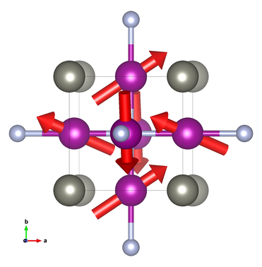
(a) PBE, trial I Converged structure:
Source-free PBE
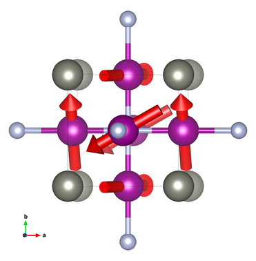
(b) PBE_SF, trial I
Trial II
Converged structure:
PBE
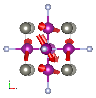
(c) PBE, trial II Converged structure:
Source-free PBE
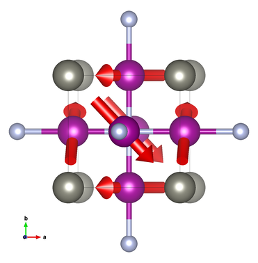
(d) PBE_SF, trial II

Figure 6: Computed ground state magnetic configurations for two input structures (trails A and B) randomly perturbed from the experimentally measured magnetic structure for Mn3ZnN; Comparisons are provided for the computed structures for PBE_SF versus PBE

Trial I
Converged structure:
PBE
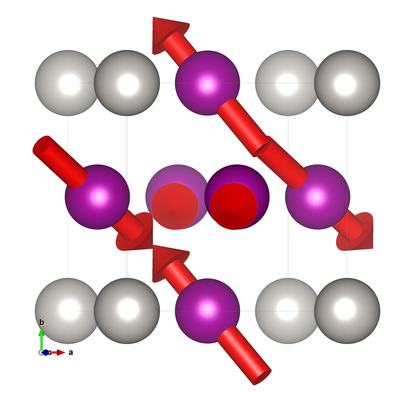
(a) PBE, trial I Converged structure:
Source-free PBE
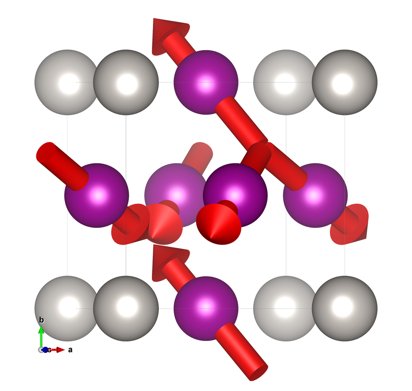
(b) PBE_SF, trial I
Trial II
Converged structure:
PBE
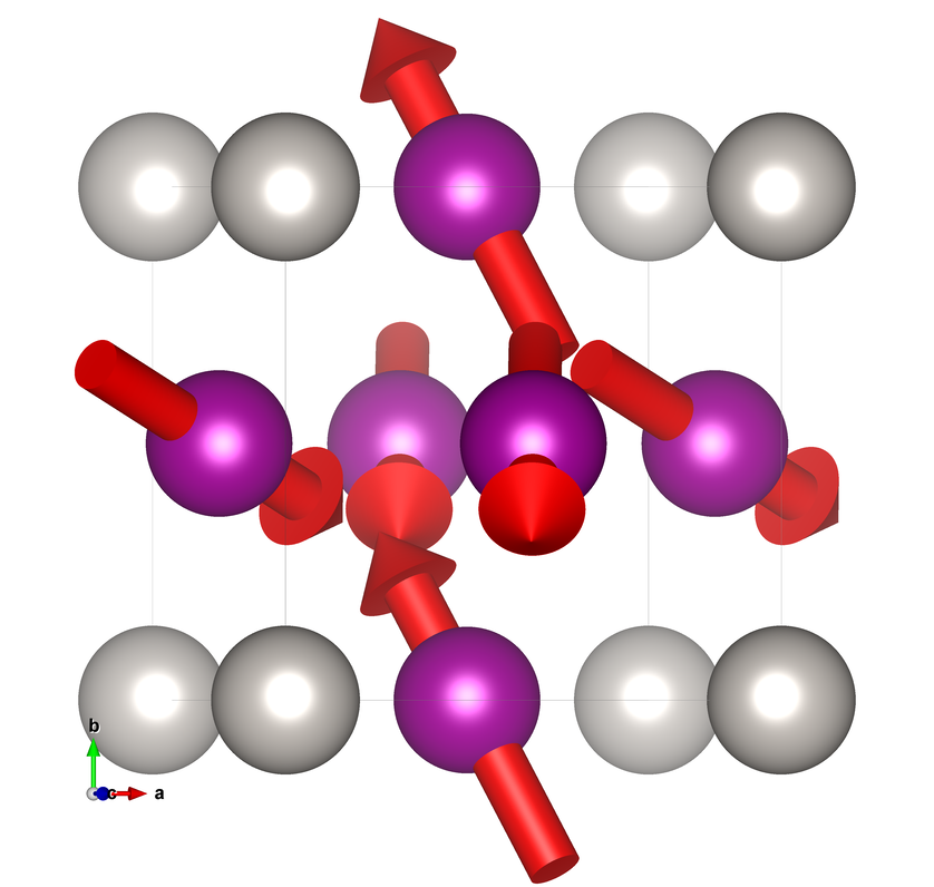
(c) PBE, trial II Converged structure:
Source-free PBE
(d) PBE_SF, trial II

Figure 7: Computed ground state magnetic configurations for two input structures (trails A and B) randomly perturbed from the experimentally measured magnetic structure for Mn3Pt; Comparisons are provided for the computed structures for PBE_SF versus PBE

Furthermore, for Mn3ZnN (Figure 6) it is clear that the curl of the magnetization, $\nabla\times\bm{m}$, varies by a much larger relative magnitude than that of Mn3Pt (Figure 7). This can be ascertained by the circulation of spins around the [1 1 1] direction in Mn3ZnN, which can be seen in Figure 1 and Figure 6 [31]. We care about a large variance in the spin current for multiple reasons. The first reason has to do with the gauge symmetries of SDFT and CDFT, as explored in Ref. 6. After all, our goal in this study is to computationally explore these degeneracies. The second reason is that the curl of the magnetization enters into the expression for the net XC torque, as stated in Equation 23. Hence, we surmise that the magnetic structure of Mn3ZnN will test the limits of the ZTT, and to what degree it is, or isn’t upheld at the point of self-consistency.

III.1 Quantifying the effects of monopoles

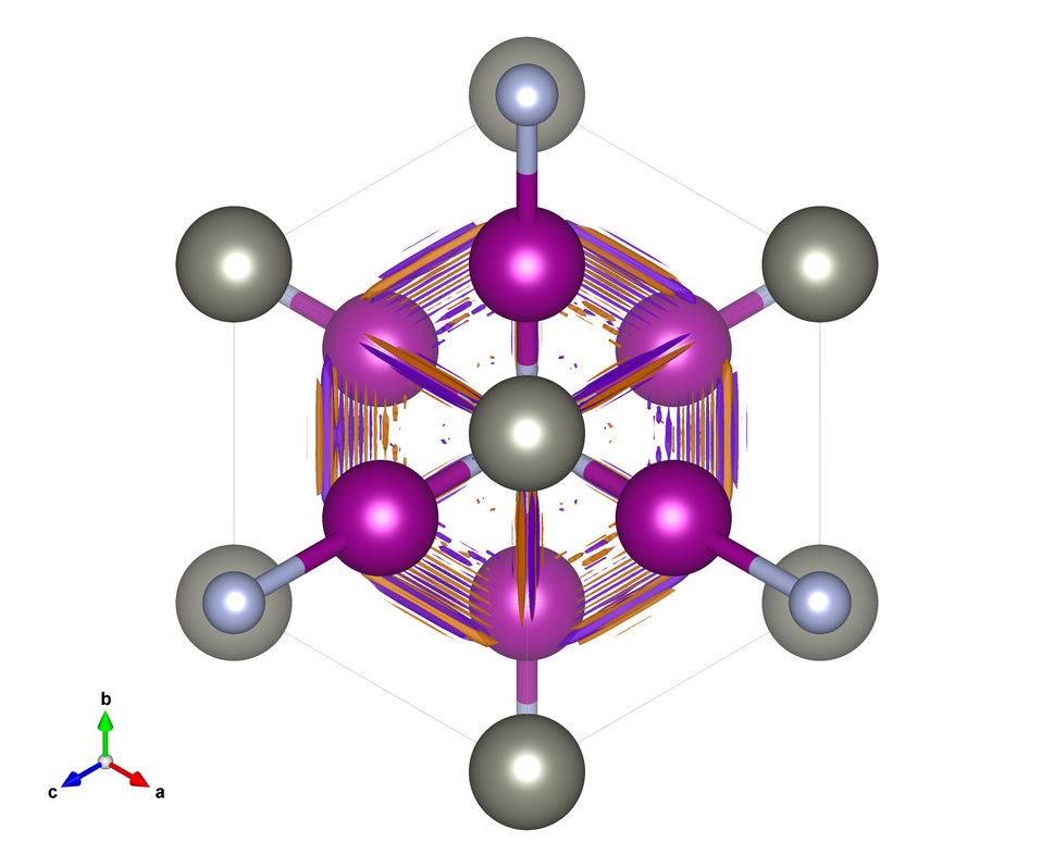
Figure 2: Isosurface VESTA plot of PBE ground state $\nabla\cdot\bm{B}_{xc}(\bm{r})$ viewed along [111] direction for Mn3ZnN. Positive isosurface is indicated in violet, and negative counterpart in orange, at a fixed isosurface level. Manganense, zinc, and nitrogen atoms are color-coded in magenta, grey, and light blue, respectively.

We found that for the Mn3ZnN calculations, the PBE+U+J calculation yielded $|\nabla\cdot\bm{B}_{xc}(\bm{r})|_{\infty}\approx$ 104 eV/($\mu_{\text{B}}$ Å⁴), and for the source-free PBE+U+J counterpart, $|\nabla\cdot\bm{B}_{xc}(\bm{r})|_{\infty}$ $<$ $10^{-13}$ eV/($\mu_{\text{B}}$ Å⁴), where $|\nabla\cdot\bm{B}_{xc}(\bm{r})|_{\infty}=\max_{\bm{r}\in\mathbb{R}^{3}}\left|\nabla\cdot\bm{B}_{xc}(\bm{r})\right|$. This numerical comparison confirms that the source-free constraint is working as expected, and draws attention to the large density of magnetic monopoles that form in conventional non-collinear PBE+U+J. A visualization of the monopole density in the Mn3ZnN test case is provided in Figure 2. We hone in on this material for reasons of computational cost and clear visualization. Namely, Mn3ZnN exhibits a highly non-collinear spin texture, describable with a commensurate unit cell of only three magnetic atoms. Furthermore, this magnetic antiperovskite is known to exhibit exceptionally large and exotic magnetostriction effects [32], which is relevant to magnetostructural phase transitions and therefore magnetocalorics [33].

III.2 Local convergence test

In order to compare the convergence of GGA-PBE_SF to conventional non-collinear GGA-PBE, we performed tests on the set of commensurate magnetic structures containing transition metal elements. To test the convergence of all structures, we apply a random perturbation from the experimental structure to all magnetic moments. The rotations of local moments are performed by an implementation of the Rodrigues’ rotation formula within a cone angle of 45°.

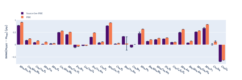
Figure 4: Comparison plot of magnetic moment differences with experiment for PBE+$U$+$J$ and PBE_SF+$U$+$J$ for a selected number of experimental structures from the MAGNDATA Bilbao Crystallographic Server [28]. The $y$-axis is the difference metric $(1/N)\sum_{i}(m^{i}_{\text{DFT}}-m^{i}_{\text{exp}})$, where $m^{i}_{\text{DFT}}$ and $m^{i}_{\text{exp}}$ are the magnetic moment magnitudes for site “$i$” from the DFT-computed and experimental magnetic structures, respectfully.

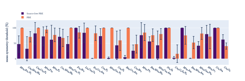
Figure 5: Comparison plot of minimum symmetry tolerance agreement with experimentally resolved magnetic space-group PBE+$U$+$J$ and PBE_SF+$U$+$J$ for a selected number of experimental structures from the MAGNDATA Bilbao Crystallographic Server [28]. The $y$-axis is the minimum symmetry tolerance (in $\mu_{\text{B}}$) at which the experimental magnetic space-group is identified, normalized by $\max_{i}\{m^{i}_{\text{exp}}\}$. We use ISOTROPY’s findsym to identify the magnetic space-group [34].

To compare the performance of the source-free functional versus its SDFT counterpart, we provide a magnetic moment comparison (in Figure 4) as well as a symmetry comparison (in Figure 5). For the magnetic moment comparison, we plot the mean difference across magnetic moments computed using GGA-PBE_SF+$U$+$J$ versus GGA-PBE+$U$+$J$. We observe that for all of these magnetic systems, the source-free functional predicts a moment that is slightly smaller than its source-free counterpart, bringing it in closer agreement with experiment, for most systems.

In order to probe the comparison between non-collinear ground states themselves, we show a symmetry metric comparison between converged structures from GGA-PBE_SF+$U$+$J$ and GGA-PBE+$U$+$J$ in Figure 5. For this study, we used the findsym program from the ISOTROPY software suite developed by Stokes et al. [34]. We define this symmetry metric to be the minimum tolerance (in $\mu_{\text{B}}$), normalized by the absolute maximum magnitude of the individual magnetic moments within the structures, and scaled as a percentage value. Therefore, 0% implies perfect agreement with experimentally resolved magnetic space-group, whereas 100% implies poor agreement. We emphasize that for this study, we use mean $U$ and $J$ values taken from Ref. 35. In principle, one should calculate these $U$ and $J$ values for each structure, as $U$ and $J$ are very sensitive to local chemical environment, and therefore oxidation and spin states [35]. However, to reduce immediate computational cost, we save this exploration for future studies.

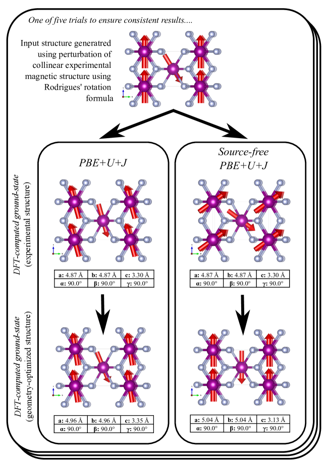
Figure 8: Computed ground state magnetic configurations for randomly perturbed input structure from the experimentally measured magnetic structure for MnF2; Comparisons are provided for the computed structures for PBE_SF versus PBE

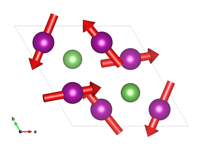
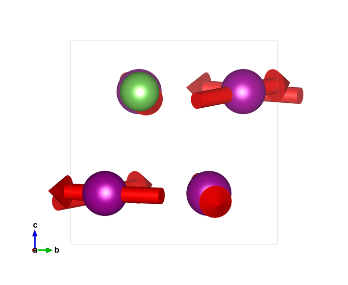
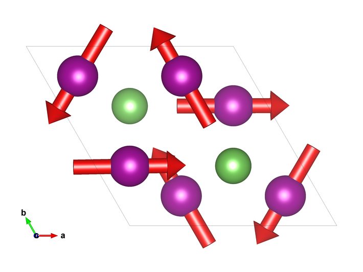
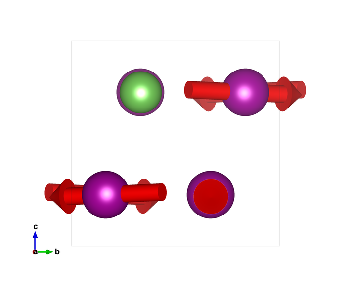
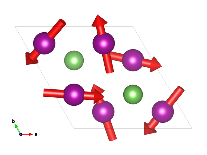
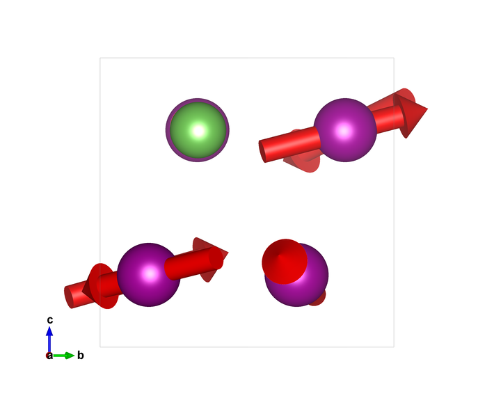
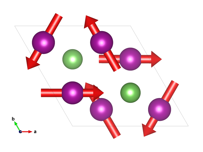
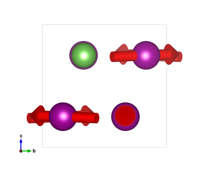
Trial I
Converged structure:
PBE (b) PBE, trial I
viewed along [001] (c) PBE, trial I
viewed along [100] Converged structure:
Source-free PBE (d) PBE_SF, trial I
viewed along [001] (e) PBE_SF, trial I
viewed along [100]
Trial II
Converged structure:
PBE (g) PBE, trial II
viewed along [001] (h) PBE, trial II
viewed along [100] Converged structure:
Source-free PBE (i) PBE_SF, trial II
viewed along [001] (j) PBE_SF, trial II
viewed along [100]

Figure 11: Computed ground state magnetic configurations for two input structures (trails A and B) randomly perturbed from the experimentally measured magnetic structure for Mn3As; Comparisons are provided for the computed structures for PBE_SF versus PBE; For PBE_SF and PBE runs, input atomic positions and cell shape were first determined by performing structural relaxations, with moments initialized in the symmetric orientation

Figures 6 and 8 show improved agreement with experimentally measured magnetic ground states using PBE_SF+$U$+$J$ compared to PBE+$U$+$J$, as well as better consistency of the output computed spin configuration. Improved performance of the SF functional is also achieved in Figures 8 and 11. In the case of MnF2 and Mn3As, we performed structural relaxations, with the spins initialized in the symmetric and/or experimental configuration. We explored the effect of structural optimization in these two materials, because without allowing for spin-lattice relaxation, a ground state with a strong ferromagnetic component was stabilized, as was the case for MnF2, which is shown in Figure 8.

III.3 Convergence case study: YMnO3

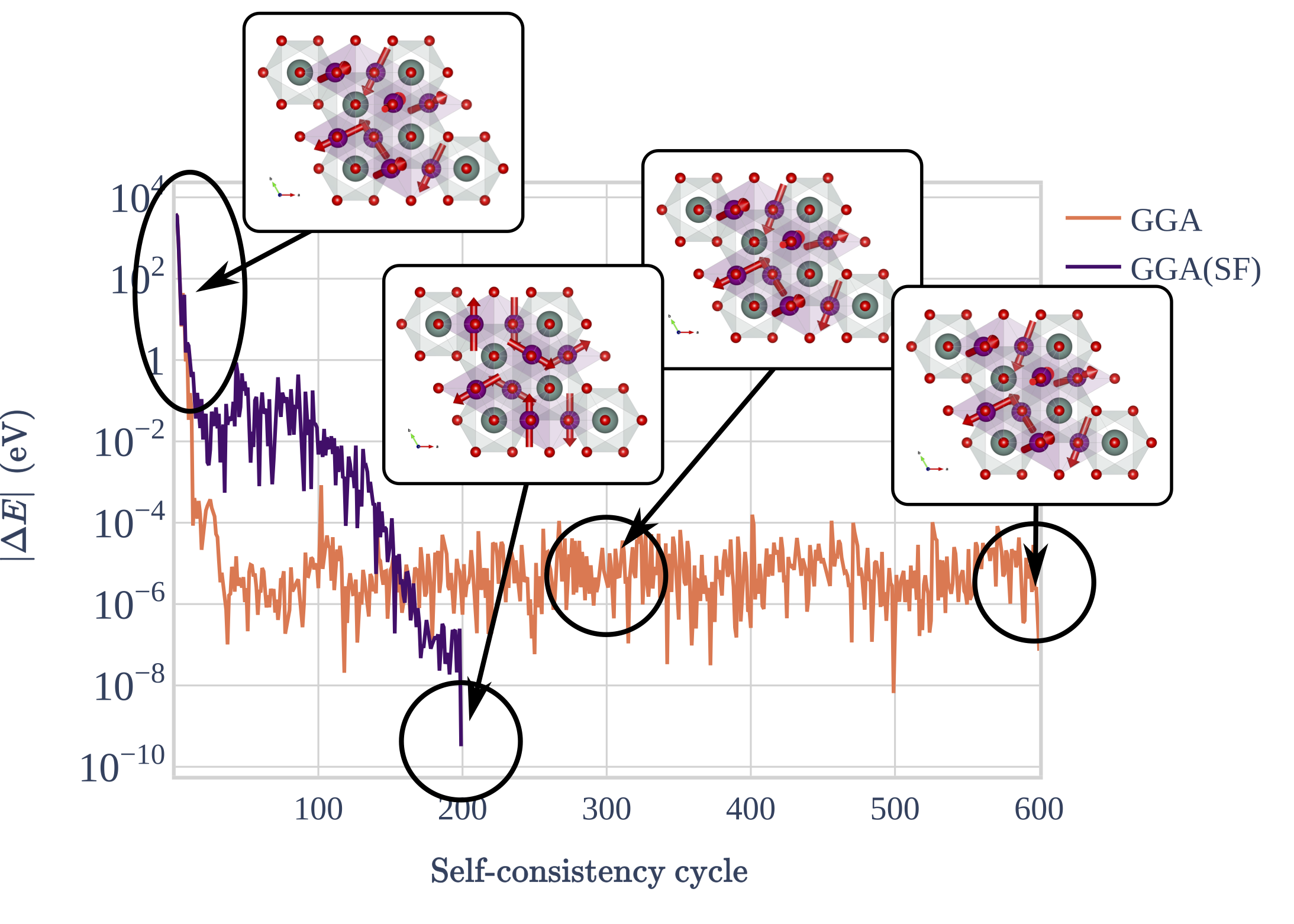
Figure 13: Convergence of GGA_SF compared against GGA for YMnO3, with moments randomly perturbed from the symmetric ground state structure. Snapshots of the magnetic configuration at each self-consistency step are shown to convey the improved convergence characteristics of the source-free functional. The $y$-axis is the absolute energy difference between subsequent self-consistency iterations, plotted on a logarithmic scale.

To examine whether a tighter energy convergence threshold improves the converged structure for GGA, we imposed a $10^{-8}$ eV energy cut off to YMnO3, comparing the convergence behavior between GGA and it source-free counterpart. The convergence behavior of GGA compared to GGA_SF is shown in Figure 13. In this plot, the absolute relative energy between subsequent self-consistency steps is plotted on a logarithmic scale. For the source-free functional, it is interesting to note that there appears to be a slight energy barrier that the algorithm climbs, only to descend to the symmetric experimentally reported ground state [8], just before 200 self-consistency steps.

To the reader, this may seem to be a long convergence time, however, we direct the attention to the conventional GGA counterpart. While convergence to 1 $\mu$eV is achieved rather rapidly, we see that the magnetic spins move very little in the convergence process. Furthermore, with the tighter energy cut off, the DFT calculation does not converge within the 600 electronic self-consistency step limit. At one point, the energy does dip below the tolerance energy threshold, but this is not simultaneously true for the band-structure convergence metric, which stays above the 0.01 $\mu$eV energy cut off.

It is worth noting that to improve convergence for this particular calculation, we used a “sigma” value smearing of 0.2 near to the Fermi level. This is standard practice, and a different smearing can be used by continuing the DFT calculation with a smaller “sigma” value, and a different smearing method. Additionally, we used Gaussian smearing, which is known to be more robust across different material chemistries, such as between insulators and conductors, according to VASP documentation.

III.4 Augmented orbital moments in UO2

Thus far, we have focused on the spin component of the magnetic moment. However, in reality, there is an orbital component to the magnetic moment that supplements the spin contribution [36, 37], especially in materials with strong spin-orbit coupling (SOC). In many $3d$ transition metal oxides, it can be theoretically and experimentally shown that the orbital moment is “quenched” [14, 38], in which case it is fair to neglect the orbital contributions. However, in $f$-block species, SOC can become much more prevalent. Additionally, we have explored the connections between the orbital moment and the paramagnetic current density, $\bm{j}_{p}$ in I.4. Therefore, it would behoove us to explore how the source-free functional affects the orbital magnetic moments.

UO2 has become the archetype of correlated oxides with strong spin-orbit coupling, which gives rise to the strongly non-collinear ground state of UO2 [39]. Therefore, we apply the source-free functional towards UO2, which we found to exhibit exceptionally large orbital magnetic moments. Specifically, we report the computed spin and orbital magnetic moments in Table 1 using GGA+$U$+$J$ and GGA_SF+$U$+$J$. Due to the connection between orbital moments and $\bm{j}_{p}$ in Equation 26, we plot $\bm{j}_{p}(\bm{r})$ in Figure 14. We see that in this visualization, there is strong circulation of $\bm{j}_{p}$ around the uranium atoms, shown in grey. It is interesting to note that we achieve this improved agreement with experiment, even without the direct coupling to $\bm{A}_{xc}$ in the form of Equation 18.

III.5 Local and global torques arising from the source-free constraint

In Figure 3a we observe that it is indeed not the case that $\bm{\tau}_{xc}^{\prime}=\bm{0}\ \forall\ \bm{r}\in\Omega$. However, for the systems we tested, we found the net (integrated) torque, as stated in Equation 23, to be orders of magnitude smaller than the largest local torque, i.e. $\max_{\bm{r}\in\Omega}\left\{\left|\bm{\tau}_{xc}^{\prime}(\bm{r})\right|\right\}$. We found that for our Mn3ZnN test case, the self-consistent $\bm{\tau}_{xc}$ obeyed the following inequality $\int_{\Omega}\bm{\tau}_{xc}\ d\bm{r}<$ $5\times 10^{-5}$ eV, even though $\max_{\Omega}\left\{\bm{\tau}_{xc}\right\}\approx$ 5 eV. The energy convergence tolerance for this calculation was $1\times 10^{-6}$ eV. Therefore, the net torque could simply be an artifact of numerical convergence.

Despite the “small” net torque relative to the energy convergence tolerance, it is nontrivial to determine whether the right-hand side of Equation 23 will be “small enough” in general. Additionally, further investigation should examine the effects of enforcing the ZTT at every self-consistency step. In Appendix A, we propose possible approaches to ensure that the ZTT is upheld at every self-consistency step. The method in Appendix A should be the most general and robust, with added computational cost. We have not implemented these ZTT corrections at this time. However, we imagine that a careful adherence to the ZTT will be important for the calculation of magnetocrystalline anisotropy energy (MAE), which is on the order of $\mu$eV, and therefore this additional physical constraint should be considered.

III.6 Importance of the constant, $\bm{q}=\bm{0}$, component of ${\bm{B}^{\prime}}_{xc}$

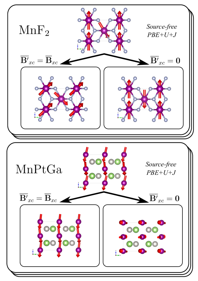
Figure 9: Comparison between the different choices of $\overline{\bm{B}^{\prime}}_{xc}$ for antiferromagnetic MnF2 (top) and canted ferromagnetic MnPtGa (bottom). Treatment of $\overline{\bm{B}^{\prime}}_{xc}$ alone can dictate the FM or AFM character of spin-polarized systems. As the inclusion of a $q=0$ component changes the Kohn-Sham effective potential, the absolute energies computed with or without $\overline{\bm{B}}_{xc}$ are not directly comparable.

In Figure 9, it is clear that when applying the $\overline{\bm{B}^{\prime}}_{xc}=\bm{0}$ constraint for MnF2, the SF functional converges to the correct collinear AFM ground state [30]. For $\overline{\bm{B}^{\prime}}_{xc}=\overline{\bm{B}}_{xc}$, the canted FM configuration is erroneously stabilized, which is remedied by structural relaxations, as shown in Figure 8. On the other hand, for MnPtGa, if one applies the additional $\overline{\bm{B}^{\prime}}_{xc}=\bm{0}$ constraint, we see that the ground state is a structure with much stronger AFM character. This differs significantly from the canted ferromagnetic configuration obtained using $\overline{\bm{B}^{\prime}}_{xc}=\overline{\bm{B}}_{xc}$. This canted FM spin configuration is much closer to the magnetic ordering resolved using neutron diffraction [40].

To generalize this behavior, $\overline{\bm{B}^{\prime}}_{xc}=\overline{\bm{B}}_{xc}$ erroneously stabilizes ferromagnetism in antiferromagnetics, and $\overline{\bm{B}^{\prime}}_{xc}=\bm{0}$ stabilizes antiferromagnetism in ferromagnets, which is equally problematic. Due to the obvious importance of carefully considering $\overline{\bm{B}^{\prime}}_{xc}$, we plan to address this in the future. For all other test cases in this study, we simply set $\overline{\bm{B}^{\prime}}_{xc}=\overline{\bm{B}}_{xc}$, in order to maintain consistency with Ref.’s 1 & 25. As we mention in the introduction, it would be possible to solve for $\overline{\bm{B}^{\prime}}_{xc}$ that mitigates the net XC torque, while preserving the XC spin-splitting energy from SDFT, in accordance with Equation 1. We plan to explore this rigorously in a follow-up study.

IV Conclusions

Significantly improved convergence to the non-collinear magnetic structure has been achieved with the application of the source-free constraint to $\bm{B}_{xc}$ [1] to the PAW DFT formulation implemented in VASP. With the use of parallel three-dimensional FFTs as the basis for the fast Poisson solver, it is possible to apply this constraint with little additional computational cost, and no reduction of the parallel scalability of the DFT code. While we have focused on GGA-PBE_SF+$U$+$J$ in this study, this constraint is generalizable to other SDFT functionals in non-collinear implementations, such as meta-GGA.

Subsequent studies will combine the improved local convergence of DFT_SF with global optimization algorithms in order to achieve a unified and robust determination of non-collinear ground states without any prior experimental knowledge.

We hope that the augmented magnetoelectric coupling predicted using the source-free functional lays the groundwork for future studies to perform an in-depth investigation of the magnetoelectric figures of merit calculated using this modified functional, especially considering that the Berry phase provides a convenient and rigorous theoretical link between the modern theory of polarization and the modern theory of magnetization [37, 36], which can be explicitly expressed in terms of the spin current [41]. Additionally, the unified theory provides a robust and solid theoretical description of the orbital magnetic moment [36], which extends the semiclassical theory touched on in Section I.4. Future studies are encouraged to further examine the role of spin and orbital currents as they pertain to magnetoelectric coupling.

V Acknowledgements

We would like to thank Dr. S. Sharma and Dr. J. K. Dewhurst for taking the time to discuss the source-free implementation over video conference call. We appreciate their support and encouragement. G.M. acknowledges support from the Department of Energy Computational Science Graduate Fellowship (DOE CSGF) under grant DE-SC0020347. Computations in this paper were performed using resources of the National Energy Research Scientific Computing Center (NERSC), a U.S. Department of Energy Office of Science User Facility operated under contract no. DE-AC02-05CH11231. Expertise in high-throughput calculations, data and software infrastructure was supported by the U.S. Department of Energy, Office of Science, Office of Basic Energy Sciences, Materials Sciences and Engineering Division under Contract DE-AC02-05CH11231: Materials Project program KC23MP.

.1 Numerical details of source-free constraint

Because plane-wave DFT is defined on periodic boundary conditions, we can start with the definition of the inverse discrete Fourier transform, because the density fields lie in regular three-dimensional grids,

$$\phi_{\bm{n}} =\frac{1}{M}\sum_{\bm{k}}\widehat{\phi}_{\bm{k}}\exp\left(i2\pi\bm{k}^{T}D^{-1}\bm{n}\right)$$

$$=\mathcal{F}^{-1}\widehat{\phi}$$ (27)

$$\text{where }D =\begin{pmatrix}N_{x}&0&0\\ 0&N_{y}&0\\ 0&0&N_{z}\\ \end{pmatrix},\text{ and }M=N_{x}N_{y}N_{z}$$

where $n_{i},k_{i}\in\left[0,1,...,N_{i}\right]$, and $N_{x},N_{y},N_{z}$ are the dimensions of the 3D grid. If we define the real-space position vector as $\bm{r}=LD^{-1}\bm{n}$, where $L$ has columns as lattice vectors $L=[\bm{a}\ \bm{b}\ \bm{c}]$. Therefore, $\bm{k}^{T}D^{-1}\bm{n}=\bm{k}^{T}D^{-1}DL^{-1}\bm{r}=\bm{k}^{T}L^{-1}\bm{r}$. From here, we can apply the convenient “scaling” property describing how differential operators commute with the inverse discrete Fourier transform, where $l=x,y,z$ is the dimension of the partial derivative,

$$\frac{\partial}{\partial r_{l}}\phi(\bm{r}) \approx i2\pi\cdot\mathcal{F}^{-1}\left(q_{l}\widehat{\phi}\right)$$ (28)

$$\text{where }q_{l} =\sum_{j}L^{-1}_{jl}k_{j},\quad\bm{q}=L^{-T}\bm{k}$$

To obtain the (discrete) spectral approximation of the divergence of the $\bm{B}$ field:

$$\nabla\cdot\bm{B}_{xc} =\frac{\partial B_{x}}{\partial x}+\frac{\partial B_{y}}{\partial y}+\frac{\partial B_{z}}{\partial z}$$

$$\approx i2\pi\cdot\mathcal{F}^{-1}\left(q_{x}\widehat{B}_{x}+q_{y}\widehat{B}_{y}+q_{z}\widehat{B}_{z}\right)$$

$$\approx i2\pi\cdot\mathcal{F}^{-1}\left(\bm{q}^{T}\widehat{\bm{B}}_{xc}\right)$$ (29)

In order to solve the Poisson equation, as posed in Equation 5, we apply a similar reasoning as before, and see that

$$\nabla^{2}\phi =\frac{\partial^{2}\phi}{\partial x^{2}}+\frac{\partial^{2}\phi}{\partial y^{2}}+\frac{\partial^{2}\phi}{\partial z^{2}}$$

$$\approx-(2\pi)^{2}\cdot\mathcal{F}^{-1}\left((q_{x}^{2}+q_{y}^{2}+q_{z}^{2})\widehat{\phi}\right)$$

$$\approx-(2\pi)^{2}\cdot\mathcal{F}^{-1}\left(|\bm{q}|^{2}\widehat{\phi}\right)$$ (30)

Therefore, combining Equations 29, 30 and 5, we find that the discrete Fourier transform of $\phi$ can be expressed as

$$\widehat{\phi}(\bm{q}) =\begin{cases}\frac{i}{2\pi}\frac{\bm{q}\cdot\widehat{\bm{B}}_{xc}(\bm{q})}{|\bm{q}|^{2}},&|\bm{q}|\neq 0\\ 0,&|\bm{q}|=0\end{cases}$$ (31)

We are interested in $\nabla\phi$. Which we can approximate as

$$-\nabla\phi \approx\mathcal{F}^{-1}\left(\frac{\bm{q}^{T}\widehat{\bm{B}}_{xc}(\bm{q})}{|\bm{q}|^{2}}\bm{q}\right)$$ (32)

Therefore, the source-free correction is achieved by performing the following

$$\widehat{\bm{B}^{\prime}}_{xc}(\bm{q})=\widehat{\bm{B}}_{xc}(\bm{q})-\begin{cases}\frac{\bm{q}\cdot\widehat{\bm{B}}_{xc}(\bm{q})}{|\bm{q}|^{2}}\bm{q},&|\bm{q}|\neq 0\\ 0,&|\bm{q}|=0\end{cases}$$ (33)

and as a result, $\nabla\cdot{\bm{B}_{xc}}^{\prime}=0$ is obtained in the discrete numerical sense.

Appendix A A general approach to satisfy the zero torque theorem

Our goal is to solve for an auxillary field $\bm{A}^{\prime}$ such that the zero torque condition is obeyed

$$\int_{\Omega}d\bm{r}\ \bm{m}\times\bm{B}=\int_{\Omega}d\bm{r}\ \bm{m}\times(\nabla\phi+\nabla\times{\bm{A}^{\prime}}) =\bm{0}.$$ (34)

The trivial solution, $\nabla\times{\bm{A}^{\prime}}=-\nabla\phi$, can only hold if $\nabla\phi=\bm{0}$. Therefore, we recast the problem as such

$$\int_{\Omega}d\bm{r}\ \bm{m}\times(\nabla\times{\bm{A}^{\prime}}) =-\int_{\Omega}d\bm{r}\ \bm{m}\times\nabla\phi=-\bm{\tau}^{\prime}.$$ (35)

By expanding the triple product, we see that

$$\bm{m}\times(\nabla\times{\bm{A}^{\prime}}) =\left[m_{j}\partial_{i}{A^{\prime}}_{j}-m_{j}\partial_{j}{A^{\prime}}_{i}\right]\hat{\bm{e}}_{i}$$

$$=\nabla_{{\bm{A}^{\prime}}}(\bm{m}\cdot{\bm{A}^{\prime}})-(\bm{m}\cdot\nabla){\bm{A}^{\prime}}.$$ (36)

At this step, we can apply the product rule, $u\partial_{x}v=\partial_{x}(uv)-v\partial_{x}u$, to show that integrals of the form $\int d\bm{r}\ \partial_{x}(uv)$ vanish under periodic boundary conditions (PBCs) by Equation SLABEL:si-eq:grad_int_periodic. Having leveraged this convenient property of the PBCs, it is possible to transfer the derivatives from $\bm{A}^{\prime}$ to $\bm{m}$ such that we can restate Equation 35 as

$$\int d\bm{r}\ \bm{m}\times(\nabla\times{\bm{A}^{\prime}})$$

$$\quad=\int d\bm{r}\ \left[{A^{\prime}}_{i}\partial_{j}m_{j}-{A^{\prime}}_{j}\partial_{i}m_{j}\right]\hat{\bm{e}}_{i}=-\bm{\tau}^{\prime}$$ (37)

Now, we will introduce the following discretized approximation for the $L^{2}$ inner product on regular grids

$$\langle u,v\rangle =\int_{\Omega}d\bm{r}\ u(\bm{r})v(\bm{r})\approx\frac{1}{\Delta V}\bm{u}^{T}\bm{v},$$ (38)

where $\Delta V=\Delta x\Delta y\Delta z$. We introduce this shorthand for the purposes of this study, however, it is just as applicable to continuous functions. With this definition, we can recast the problem in Equation 37 as a matrix-vector system

$$M\bm{a}=-\bm{\tau}^{\prime},$$ (39)

where $\bm{a}=\left[{\bm{A}^{\prime}}_{x}^{T}\ {\bm{A}^{\prime}}_{y}^{T}\ {\bm{A}^{\prime}}_{z}^{T}\right]^{T}$, and the matrix $M$ is defined as

$$M =\frac{1}{\Delta V}\begin{bmatrix}{\bm{m}}_{y,y}^{T}+{\bm{m}}_{z,z}^{T}&-{\bm{m}}_{y,x}^{T}&-{\bm{m}}_{z,x}^{T}\\ -{\bm{m}}_{x,y}^{T}&{\bm{m}}_{z,z}^{T}+{\bm{m}}_{x,x}^{T}&-{\bm{m}}_{z,y}^{T}\\ -{\bm{m}}_{x,z}^{T}&-{\bm{m}}_{y,z}^{T}&{\bm{m}}_{x,x}^{T}+{\bm{m}}_{y,y}^{T}\end{bmatrix},$$ (40)

in which case $\bm{m}_{i,j}=\frac{\partial\bm{m}_{i}}{\partial x_{j}}$. Because the system of equations is underdetermined (i.e. $M$ is “short and fat”), we can can solve for $\bm{a}$ using a least-squares approach,

$$\bm{a} =-M^{+}\bm{\tau}^{\prime},$$ (41)

which solves for the solution $\bm{a}$ with minimal $L^{2}$ norm,

$$||\bm{a}||_{2}=\left\{\sum_{i=x,y,z}\int_{\Omega}d\bm{r}\ |\bm{A}^{\prime}_{i}(\bm{r})|^{2}\right\}^{1/2}.$$ (42)

$M^{+}$ is the correspanding Moore-Penrose right-hand pseudoinverse $M^{+}=M^{T}\left(MM^{T}\right)^{-1}$ such that $MM^{+}=I$, as long as the rows of $M$ are linearly independent. We note that $MM^{T}$ is diagonally dominant, because it contains $L^{2}$ norms (which are guaranteed to be positive) of the spatial partial derivatives of $\bm{m}$ along the diagonal. Therefore, $MM^{T}$ should be invertible, so long as the magnetization varies in all spatial directions over the domain, which it should for spin-polarized systems.

In conclusion, by applying both source-free and ZTT corrections to the exchange-correlation magnetic field, $\bm{B}_{xc}$,

$$\bm{B}_{xc} \mapsto{\bm{B}^{\prime}}_{xc}$$

$${\bm{B}^{\prime}}_{xc} =\bm{B}_{xc}+\nabla\phi+\nabla\times{\bm{A}^{\prime}}$$ (43)

we can simultaneously satisfy

1. The source free constraint:

   $$\nabla\cdot{\bm{B}^{\prime}}_{xc}=0$$

2. The zero torque theorem:

   $$\int_{\Omega}d\bm{r}\ \bm{m}\times{\bm{B}^{\prime}}_{xc}=\bm{0}.$$

However, we should stress that the second ZTT constraint is not implemented in the code at present. In other words, we set $\bm{A}^{\prime}(\bm{r})=\bm{0}$ in the context of this study.

Appendix B Choice of $\bm{A}_{xc}$ gauge

It is worth noting that two gauge choices of $\bm{A}_{xc}$ have been presented in the literature. Within the original works of Vignale and Rasolt [9, 11, 16], the $\nabla\cdot\left(\rho\bm{A}_{xc}\right)=0$ arises naturally. However, by comparison, in [6], the Coulomb gauge $\nabla\cdot\bm{A}_{xc}=0$ is implied by the Helmholtz decomposition.

Under the $\nabla\cdot\bm{A}_{xc}=0$ gauge, it is possible to solve for $\bm{A}_{xc}$ using the following Poisson equation,

$$\nabla\times\left(\nabla\times\bm{A}_{xc}\right) =\nabla\times\bm{B}_{xc}$$

$$-\nabla^{2}\bm{A}_{xc}+\nabla\left(\nabla\cdot\bm{A}_{xc}\right) =\nabla\times\bm{B}_{xc}$$

$$\nabla^{2}\bm{A}_{xc} =-\nabla\times\bm{B}_{xc}$$ (44)

In order to solve for $\bm{A}_{xc}$ subject to $\nabla\cdot\left(\rho\bm{A}_{xc}\right)=0$, we can employ another Helmholtz decomposition

$$\bm{A}_{xc} =\bm{A}_{xc}^{\prime}+\nabla\xi$$

where $\nabla\cdot\bm{A}_{xc}^{\prime}=0$ and is solved using Equation 44, and $\xi$ is determined from the following elliptical equation

$$\nabla\cdot\left(\rho\nabla\xi\right) =-\nabla\cdot\left(\rho\bm{A}_{xc}^{\prime}\right).$$ (46)

However, the spatial dependence of $\rho$ in Equation 46 makes the equation more difficult to solve using a single spectral solve step. Instead, an iterative spectral solver could be used to solve this elliptical equation, using the subtractive solver presented in Ref. 42, for example.

Appendix C Considerations for $\bm{j}_{p}\cdot\bm{A}_{xc}$ energy contributions under periodic boundary conditions

We will use the following result, Equation 47, to draw a few conclusions.

$$\int_{\Omega}\nabla\alpha(\bm{r})\cdot\bm{L}(\bm{r})\ d\bm{r}$$

$$=\int_{\Omega}\left\{\nabla\cdot\left[\alpha(\bm{r})\bm{L}(\bm{r})\right]-\alpha(\bm{r})\left[\nabla\cdot\bm{L}(\bm{r})\right]\right\}\ d\bm{r}$$

$$=\oint_{\partial\Omega}\left[\alpha(\bm{r})\bm{L}(\bm{r})\right]\cdot d\bm{S}-\int_{\Omega}\alpha(\bm{r})\left[\nabla\cdot\bm{L}(\bm{r})\right]\ d\bm{r}$$ (47)

If $\Omega$ obeys periodic boundary conditions, then $\oint_{\partial\Omega}\left[\alpha(\bm{r})\bm{L}(\bm{r})\right]\cdot d\bm{S}=0$.

We can start by considering the Coulomb gauge $\nabla\cdot\bm{A}_{xc}=0$. If this gauge is chosen, charge conservation should still be obeyed through the following

$$\nabla\cdot\left(\bm{j}_{p}+\rho\bm{A}_{xc}\right) =0$$ (48)

By the Helmholtz identity, we can decompose $\bm{j}_{p}$ into the following

$$\bm{j}_{p}=\nabla\eta+\nabla\times\bm{\Gamma}.$$ (49)

Therefore, we may rewrite Equation 48 as

$$\nabla^{2}\eta=-\nabla\cdot\left(\rho\bm{A}_{xc}\right)$$ (50)

Here, it is interesting to note that while $\eta$ can satisfy charge conservation, by Equation 47, under periodic boundary conditions and the $\nabla\cdot\bm{A}_{xc}=0$ gauge, the following is true

$$\int_{\Omega}\nabla\eta\cdot\bm{A}_{xc}\ d\bm{r}=0.$$ (51)

Therefore, $\eta$ will not enter into the energy term, Equation 18, allowing us to conclude that

$$\left.E_{p}\right|_{\nabla\cdot\bm{A}_{xc}=0} =\int_{\Omega}\left(\nabla\times\bm{\Gamma}\right)\cdot\bm{A}_{xc}\ d\bm{r}$$

$$\qquad\forall\ \left\{\bm{j}_{p},\ \left.\bm{A}_{xc}\right|_{\nabla\cdot\bm{A}_{xc}=0}\right\}\ .$$ (52)

Equation 52 states that while the curl-free projection of $\bm{j}_{p}$, $\nabla\eta$, maintains local charge conservation, only the divergence-free projection, $\nabla\times\bm{\Gamma}$, enters into the expression for $E_{p}$.

Appendix D Considerations for $\bm{j}_{p,\lambda}$

Starting from a Helmholtz decomposition of the probability current density

$$\bm{j}_{p,\lambda} =\nabla\eta_{\lambda}+\nabla\times\bm{\Gamma}_{\lambda}$$ (53)

We see that the following conservation law

$$\nabla\cdot\left[\bm{j}_{p,\lambda}+m_{\lambda}\bm{A}_{xc}\right]=\left(\bm{m}\times\bm{B}_{xc}\right)_{\lambda}$$ (54)

only places a constraint on the curl-free contribution to $\bm{j}_{p,\lambda}$, similarly to Equation 50,

$$\nabla^{2}\eta_{\lambda} =-\nabla\cdot\left[m_{\lambda}\bm{A}_{xc}\right]+\left(\bm{m}\times\bm{B}_{xc}\right)_{\lambda}.$$ (55)

Therefore, only the divergence-free component, $\nabla\times\bm{\Gamma}_{\lambda}$, is independent from this conservation law, and will contribute to the energy in an analogous form of Equation 52.

(a) PBE_SF

(b) PBE

Figure 1: PBE_SF versus PBE comparison plot of ground state magnetization density $\bm{m}(\bm{r})$ (vector field) and $\bm{B}_{xc}(\bm{r})$ (streamlines) viewed along [111] direction for Mn3ZnN

(a) PBE_SF

(b) PBE

Figure 3: PBE_SF versus PBE comparison plot of ground state magnetic torque vector field $\bm{\tau}_{xc}=\bm{m}(\bm{r})\times\bm{B}_{xc}(\bm{r})$ (vector field) viewed along [111] direction for Mn3ZnN. The units are in ($\mu_{\text{B}}$ eV)/($\mu_{\text{B}}$ ų).

Trial I
Converged structure:
PBE
(a) PBE, trial I Converged structure:
Source-free PBE
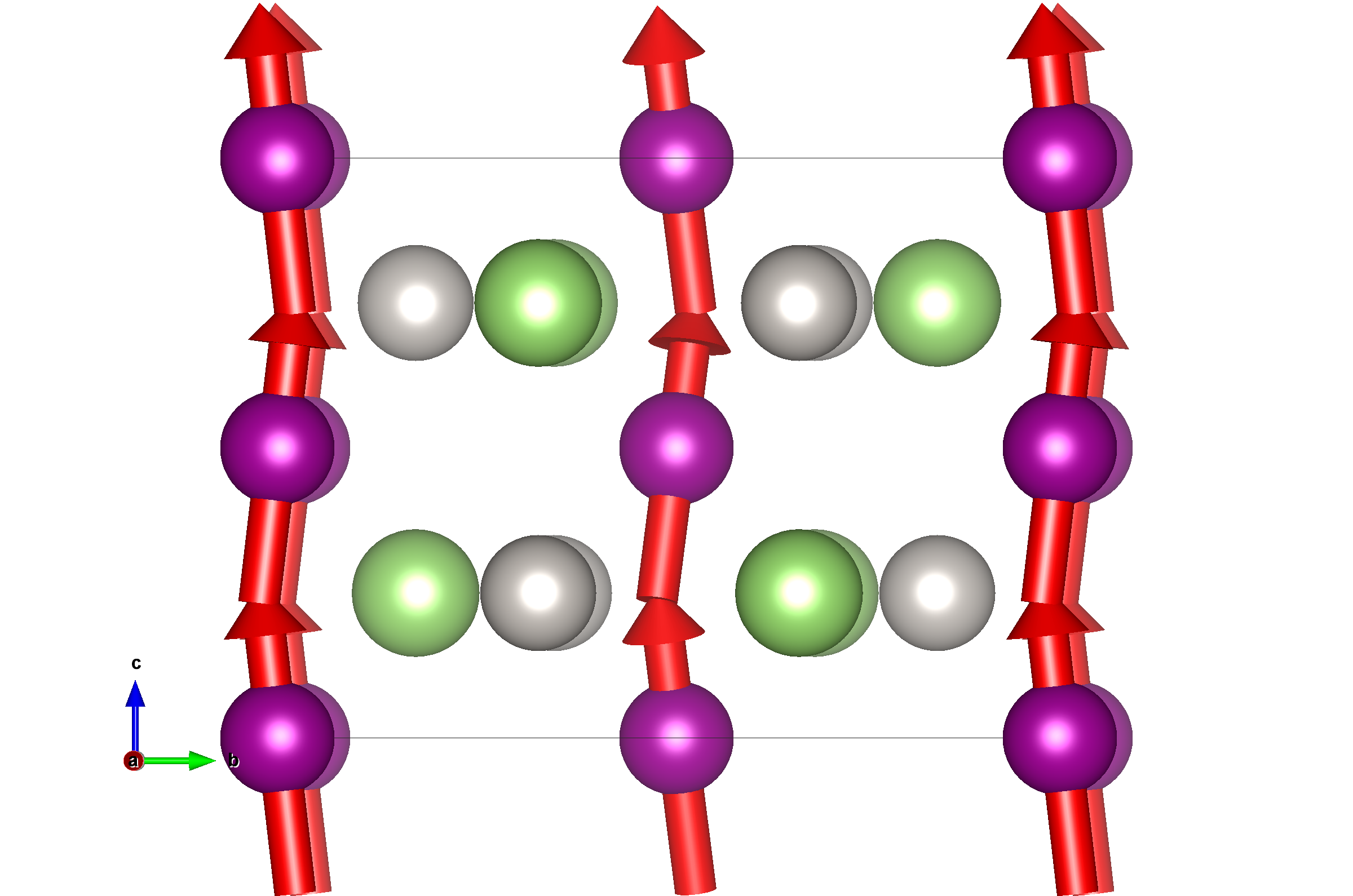
(b) PBE_SF, trial I
Trial II
Converged structure:
PBE
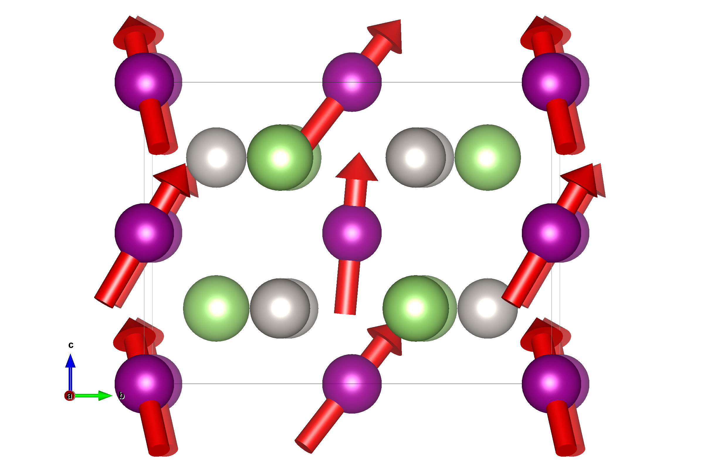
(c) PBE, trial II Converged structure:
Source-free PBE
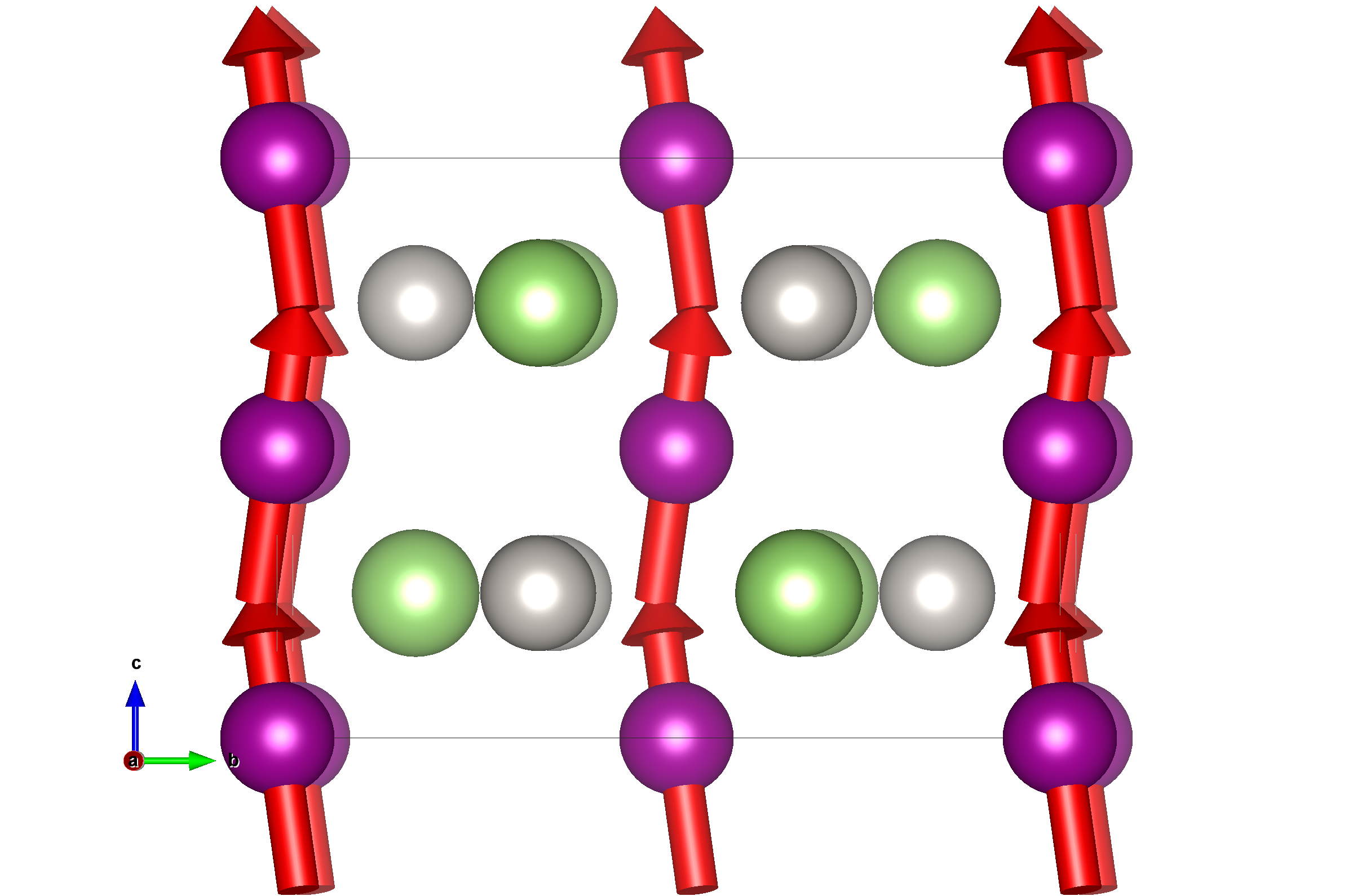
(d) PBE_SF, trial II

Figure 10: Computed ground state magnetic configurations for two input structures (trails A and B) randomly perturbed from the experimentally measured magnetic structure for MnPtGa; Comparisons are provided for the computed structures for PBE_SF versus PBE

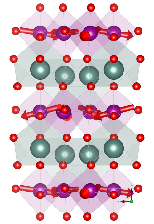
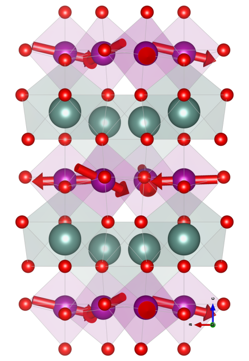
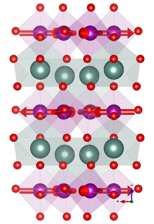
Trial I
Converged structure:
PBE
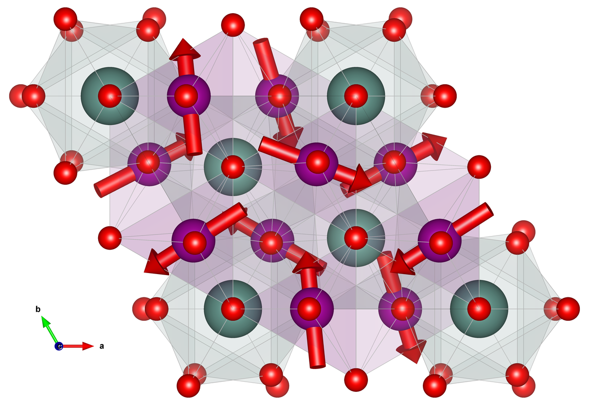
(a) PBE, trial I
viewed along [001] (b) PBE, trial I
viewed along [010] Converged structure:
Source-free PBE
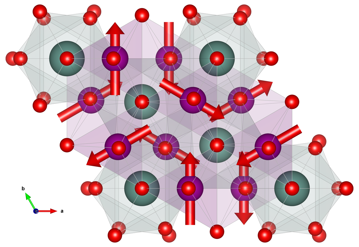
(c) PBE_SF, trial I
viewed along [001] (d) PBE_SF, trial I
viewed along [010]
Trial II
Converged structure:
PBE
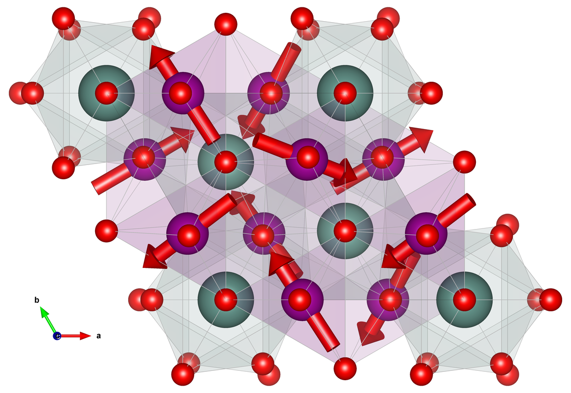
(e) PBE, trial I
viewed along [001] (f) PBE, trial I
viewed along [010] Converged structure:
Source-free PBE
(g) PBE_SF, trial I
viewed along [001] (h) PBE_SF, trial I
viewed along [010]

Figure 12: Computed ground state magnetic configurations for two input structures (trails A and B) randomly perturbed from the experimentally measured magnetic structure for YMnO3; Comparisons are provided for the computed structures for PBE_SF versus PBE; For PBE_SF and PBE runs, input atomic positions and cell shape were first determined by performing structural relaxations, with moments initialized in the symmetric orientation

Figure 14: Vector field visualization of the probability current density, $\bm{j}_{p}$, within UO2. Strong circulation of $\bm{j}_{p}$ is observed surrounding the uranium atoms, in grey.

Table 1: Tabulated magnetic moment components of the four uranium atoms in the magnetic unit cell of UO2. The spin and orbital contributions to the total computed moments by VASP are included below, computed using both PBE_SF+$U$+$J$ and PBE+$U$+$J$. The on-site corrections of $U,J=3.46,0.3$ eV were applied to U-$f$ states to maintain consistency with Ref. 43. Additionally, we compare to $U,J=4.5,1.0$ eV, which is the largest $U$ value reported in Ref. 43, and a “rounded-up” $J$ value of 1.0 eV to examine the effect of a larger Hund $J$ parameter on the spin and orbital uranium magnetic moments.

Functional	Atom	Spin				Orbital				Total
		$m_{x}$	$m_{y}$	$m_{z}$	$|\bm{m}|$	$m_{x}$	$m_{y}$	$m_{z}$	$|\bm{m}|$	$m_{x}$	$m_{y}$	$m_{z}$	$|\bm{m}|$
PBE+$U$+$J$ $U,J=3.46,0.30$ eV	I	-0.577	-0.583	-0.581	1.01	1.764	1.783	1.778	3.07	1.19	1.20	1.20	2.07
	II	-0.584	0.576	0.581	1.01	1.787	-1.763	-1.776	3.08	1.20	-1.19	-1.20	2.07
	III	0.578	-0.568	0.594	1.00	-1.769	1.739	-1.817	3.07	-1.19	1.17	-1.22	2.07
	IV	0.599	0.571	-0.57	1.00	-1.831	-1.747	1.744	3.07	-1.23	-1.18	1.17	2.07
PBE+$U$+$J$ $U,J=4.5,1.0$ eV	I	-0.19	-0.19	-0.20	0.34	1.41	1.42	1.43	2.46	1.22	1.23	1.23	2.12
	II	-0.20	0.20	0.19	0.34	1.43	-1.43	-1.40	2.46	1.24	-1.23	-1.21	2.12
	III	0.19	-0.19	0.20	0.34	-1.40	1.39	-1.47	2.46	-1.21	1.20	-1.27	2.12
	IV	0.21	0.19	-0.18	0.34	-1.51	-1.40	1.35	2.46	-1.30	-1.21	1.16	2.12
PBESF+$U$+$J$ $U,J=3.46,0.30$ eV	I	0.21	0.17	0.24	0.36	0.73	0.73	0.81	1.31	0.93	0.90	1.04	1.66
	II	0.21	-0.23	-0.19	0.36	0.73	0.73	-0.67	1.23	0.94	0.50	-0.86	1.37
	III	-0.18	0.19	-0.24	0.36	-0.66	-0.66	-0.83	1.25	-0.84	-0.47	-1.07	1.44
	IV	-0.21	-0.21	0.21	0.36	-0.73	-0.73	0.74	1.26	-0.93	-0.93	0.94	1.62
PBESF+$U$+$J$ $U,J=4.5,1.0$ eV	I	0.08	0.08	0.09	0.14	0.95	0.91	1.04	1.68	1.03	0.98	1.13	1.82
	II	0.08	-0.08	-0.08	0.14	0.99	-0.99	-0.92	1.68	1.07	-1.07	-1.00	1.82
	III	-0.08	0.08	-0.09	0.14	-0.96	0.91	-1.03	1.68	-1.04	0.99	-1.12	1.82
	IV	-0.08	-0.08	0.08	0.14	-0.94	-1.01	0.96	1.68	-1.01	-1.09	1.04	1.82

References

- Sharma et al. [2018] S. Sharma, E. K. U. Gross, A. Sanna, and J. K. Dewhurst, Source-Free Exchange-Correlation Magnetic Fields in Density Functional Theory, Journal of Chemical Theory and Computation 14, 1247 (2018).
- Krishna et al. [2019] J. Krishna, N. Singh, S. Shallcross, J. K. Dewhurst, E. K. U. Gross, T. Maitra, and S. Sharma, Complete description of the magnetic ground state in spinel vanadates, Physical Review B 100, 081102 (2019).
- Peralta et al. [2007] J. E. Peralta, G. E. Scuseria, and M. J. Frisch, Noncollinear magnetism in density functional calculations, Physical Review B 75, 125119 (2007).
- Furness et al. [2015] J. W. Furness, J. Verbeke, E. I. Tellgren, S. Stopkowicz, U. Ekström, T. Helgaker, and A. M. Teale, Current Density Functional Theory Using Meta-Generalized Gradient Exchange-Correlation Functionals, Journal of Chemical Theory and Computation 11, 4169 (2015).
- Tchenkoue et al. [2019] M.-L. M. Tchenkoue, M. Penz, I. Theophilou, M. Ruggenthaler, and A. Rubio, Force Balance Approach for Advanced Approximations in Density Functional Theories, The Journal of Chemical Physics 151, 154107 (2019), arXiv:1908.02733 .
- Capelle and Gross [1997] K. Capelle and E. K. U. Gross, Spin-Density Functionals from Current-Density Functional Theory and Vice Versa:A Road towards New Approximations, Physical Review Letters 78, 1872 (1997).
- Eschrig et al. [1985] H. Eschrig, G. Seifert, and P. Ziesche, Current density functional theory of quantum electrodynamics, Solid State Communications 56, 777 (1985).
- Muñoz et al. [2000] A. Muñoz, J. A. Alonso, M. J. Martínez-Lope, M. T. Casáis, J. L. Martínez, and M. T. Fernández-Díaz, Magnetic structure of hexagonal \ceRMnO3 (R = Y, Sc): Thermal evolution from neutron powder diffraction data, Physical Review B 62, 9498 (2000), publisher: American Physical Society.
- Vignale et al. [1990] G. Vignale, M. Rasolt, and D. J. W. Geldart, Magnetic Fields and Density Functional Theory, in Advances in Quantum Chemistry, Density Functional Theory of Many-Fermion Systems, Vol. 21, edited by P.-O. Löwdin (Academic Press, 1990) pp. 235–253.
- Sakurai and Napolitano [2017] J. J. Sakurai and J. Napolitano, Modern Quantum Mechanics, 2nd ed. (Cambridge University Press, 2017).
- Vignale and Rasolt [1987] G. Vignale and M. Rasolt, Density-functional theory in strong magnetic fields, Physical Review Letters 59, 2360 (1987).
- Steiner et al. [2016] S. Steiner, S. Khmelevskyi, M. Marsmann, and G. Kresse, Calculation of the magnetic anisotropy with projected-augmented-wave methodology and the case study of disordered alloys, Phys. Rev. B 93, 224425 (2016).
- Bencheikh [2003] K. Bencheikh, Spin–orbit coupling in the spin-current-density-functional theory, Journal of Physics A: Mathematical and General 36, 11929 (2003).
- Ashcroft and Mermin [1976] N. W. Ashcroft and D. N. Mermin, Solid state physics (Brooks/Cole, Australia, 1976 - 1976).
- Tao [2005] J. Tao, Explicit inclusion of paramagnetic current density in the exchange-correlation functionals of current-density functional theory, Physical Review B 71, 205107 (2005).
- Vignale and Rasolt [1988] G. Vignale and M. Rasolt, Current- and spin-density-functional theory for inhomogeneous electronic systems in strong magnetic fields, Physical Review B 37, 10685 (1988).
- Pluhar and Ullrich [2019] E. A. Pluhar and C. A. Ullrich, Exchange-correlation magnetic fields in spin-density-functional theory, Physical Review B 100, 125135 (2019).
- Capelle et al. [2001] K. Capelle, G. Vignale, and B. L. Gyorffy, Spin currents and spin dynamics in time-dependent density-functional theory, Physical Review Letters 87, 206403 (2001), arXiv:cond-mat/0106021 .
- Wu et al. [1992] Y. Wu, J. Stöhr, B. D. Hermsmeier, M. G. Samant, and D. Weller, Enhanced orbital magnetic moment on co atoms in Co/Pd multilayers: A magnetic circular x-ray dichroism study, Phys. Rev. Lett. 69, 2307 (1992).
- Elnaggar et al. [2019] H. Elnaggar, P. Sainctavit, A. Juhin, S. Lafuerza, F. Wilhelm, A. Rogalev, M.-A. Arrio, C. Brouder, M. van der Linden, Z. Kakol, M. Sikora, M. W. Haverkort, P. Glatzel, and F. M. F. de Groot, Noncollinear ordering of the orbital magnetic moments in magnetite, Phys. Rev. Lett. 123, 207201 (2019).
- Sharma et al. [2007] S. Sharma, S. Pittalis, S. Kurth, S. Shallcross, J. K. Dewhurst, and E. K. U. Gross, Comparison of exact-exchange calculations for solids in current-spin-density- and spin-density-functional theory, Physical Review B 76, 100401 (2007).
- sf- [2023] Source-free code patch repository, https://github.com/guymoore13/source_free_Bxc_VASP (2023).
- Note [1] After all, Sharma et al. describe the scaling as an “additional modification” to the XC functional [1]. This was further confirmed in conversation with S. Sharma and J. K. Dewhurst.
- Hafner and Kresse [1997] J. Hafner and G. Kresse, The Vienna Ab-Initio Simulation Program VASP: An Efficient and Versatile Tool for Studying the Structural, Dynamic, and Electronic Properties of Materials, in Properties of Complex Inorganic Solids, edited by A. Gonis, A. Meike, and P. E. A. Turchi (Springer US, Boston, MA, 1997) pp. 69–82.
- Hawkhead et al. [2023] Z. Hawkhead, N. Gidopoulos, S. J. Blundell, S. J. Clark, and T. Lancaster, First-principles calculations of magnetic states in pyrochlores using a source-corrected exchange and correlation functional (2023), arXiv:2302.08564 [cond-mat.mtrl-sci] .
- elk [2023] Elk codebase, https://elk.sourceforge.io (2023).
- [27] J. K. Dewhurst and S. Sharma, Development of the Elk LAPW Code, Max Planck Institute of Microstructure Physics Theory Department .
- Perez-Mato et al. [2011] J. Perez-Mato, D. Orobengoa, E. Tasci, G. De la Flor Martin, and A. Kirov, Crystallography online: Bilbao crystallographic server, Bulgarian Chemical Communications 43, 183 (2011).
- Krén et al. [2004] E. Krén, G. Kádár, L. Pál, and P. Szabó, Investigation of the First‐Order Magnetic Transformation in \ceMn3Pt, Journal of Applied Physics 38, 1265 (2004).
- Yamani et al. [2010] Z. Yamani, Z. Tun, and D. H. Ryan, Neutron scattering study of the classical antiferromagnet \ceMnF2: a perfect hands-on neutron scattering teaching issue on Neutron Scattering in Canada., Canadian Journal of Physics 88, 771 (2010), publisher: NRC Research Press.
- Fruchart et al. [1971] D. Fruchart, E. F. Bertaut, R. Madar, and R. Fruchart, Diffraction neutronique de \ceMn3ZnN, Le Journal de Physique Colloques 32, C1 (1971), publisher: EDP Sciences.
- Hamada and Takenaka [2012] T. Hamada and K. Takenaka, Phase instability of magnetic ground state in antiperovskite \ceMn3ZnN: Giant magnetovolume effects related to magnetic structure, Journal of Applied Physics 111, 07A904 (2012), publisher: American Institute of Physics.
- Law et al. [2018] J. Y. Law, V. Franco, L. M. Moreno-Ramírez, A. Conde, D. Y. Karpenkov, I. Radulov, K. P. Skokov, and O. Gutfleisch, A quantitative criterion for determining the order of magnetic phase transitions using the magnetocaloric effect, Nature Communications 9, 2680 (2018), number: 1 Publisher: Nature Publishing Group.
- [34] H. T. Stokes, D. M. Hatch, and B. J. Campbell, ISOTROPY Software Suite.
- Moore et al. [2022] G. C. Moore, M. K. Horton, A. M. Ganose, M. Siron, E. Linscott, D. D. O’Regan, and K. A. Persson, High-throughput determination of Hubbard U and Hund J values for transition metal oxides via linear response formalism (2022), arXiv:2201.04213 [cond-mat].
- Resta [2010] R. Resta, Electrical polarization and orbital magnetization: the modern theories, Journal of Physics: Condensed Matter 22, 123201 (2010).
- Chang and Niu [2008] M.-C. Chang and Q. Niu, Berry curvature, orbital moment, and effective quantum theory of electrons in electromagnetic fields, Journal of Physics: Condensed Matter 20, 193202 (2008).
- Streltsov and Khomskii [2017] S. V. Streltsov and D. I. Khomskii, Orbital physics in transition metal compounds: new trends, Physics-Uspekhi 60, 1121 (2017), publisher: IOP Publishing.
- Borovik-Romanov et al. [2013] A. S. Borovik-Romanov, H. Grimmer, and M. Kenzelmann, Chapter 1.5. Magnetic properties, in International Tables for Crystallography, Vol. D (2013) publisher: International Union of Crystallography.
- Cooley et al. [2020] J. A. Cooley, J. D. Bocarsly, E. C. Schueller, E. E. Levin, E. E. Rodriguez, A. Huq, S. H. Lapidus, S. D. Wilson, and R. Seshadri, Evolution of noncollinear magnetism in magnetocaloric MnPtGa, Physical Review Materials 4, 044405 (2020), publisher: American Physical Society.
- Katsura et al. [2005] H. Katsura, N. Nagaosa, and A. V. Balatsky, Spin current and magnetoelectric effect in noncollinear magnets, Phys. Rev. Lett. 95, 057205 (2005).
- Braverman et al. [2004] E. Braverman, B. Epstein, M. Israeli, and A. Averbuch, A Fast Spectral Subtractional Solver for Elliptic Equations, Journal of Scientific Computing 21, 91 (2004).
- Dudarev et al. [2019] S. L. Dudarev, P. Liu, D. A. Andersson, C. R. Stanek, T. Ozaki, and C. Franchini, Parametrization of LSDA+ for noncollinear magnetic configurations: Multipolar magnetism in \ceUO2, Physical Review Materials 3, 083802 (2019).