Anomalous Linear and Quadratic Nodeless Surface Dirac Cones
in Three-Dimensional Dirac Semimetals

Abstract

Surface Dirac cones in three-dimensional topological insulators have generated tremendous and enduring interest for almost two decades owing to hosting a multitude of exotic properties. In this work, we explore the topological surface states in two representative types of three-dimensional Dirac semimetals, and unveil the existence of two types of anomalous surface Dirac cones on the largely overlooked surfaces where the projections of bulk Dirac nodes overlap. These surface Dirac cones are found to display a number of features remarkably different from that in topological insulators. The most prominent one is the absence of Dirac node in them. In addition, the spin textures of these nodeless surface Dirac cones are found to exhibit a unique two-phase-angle dependence, leading to the presence of two different winding numbers in the orbital-resolved spin textures, which is rather different from the well-known spin-momentum locking in topological insulators. Despite the absence of Dirac node, we find that the surface Dirac cones are also characterized by quantized $\pi$ Berry phases, even though one type of the surface Dirac cones takes a quadratic dispersion. In the presence of time-reversal-symmetry-breaking fields, we find that the responses of the surface and bulk Dirac cones display an interesting bulk-surface correspondence. The uncovering of these nodeless surface Dirac cones broadens our understanding of the topological surface states and bulk-boundary correspondence in Dirac semimetals, and could further fuel the research interest in Dirac physics.

Since the rise of graphene and topological insulators (TIs), the exploration of Dirac-cone band structures has continued to be at the frontier of a number of disciplines Novoselov et al. (2004); Kane and Mele (2005a, b); Bernevig and Zhang (2006); Bernevig et al. (2006); Hasan and Kane (2010); Qi and Zhang (2011); Vafek and Vishwanath (2014); Armitage et al. (2018); Lu et al. (2014); Ozawa et al. (2019); Ma et al. (2019); Xue et al. (2022). The great interest in Dirac-cone band structures lies in many aspects, such as their relativistic linear dispersions Novoselov et al. (2005), their fundamental connection with topology Jackiw and Rebbi (1976); Ryu et al. (2010); Chiu et al. (2016), and being the sources of a diversity of unconventional responses Cheng et al. (2010); Tse and MacDonald (2010); Garate and Franz (2010); Xiong et al. (2015); Wu et al. (2016); Li et al. (2016); Yuan et al. (2018, 2020). The Dirac cones can be roughly classified into two classes, gapped or gapless, with the former (latter) effectively described by a massive (massless) Dirac Hamiltonian Shen (2013); Bernevig and Hughes (2013). A fundamental difference between them is that the gapless Dirac cones carry a symmetry-protected band degeneracy (known as Dirac node or point) that acts as a topological charge. As stable Dirac nodes requires symmetry protection, it is known that the lattice realization of gapless Dirac cones faces the fermion-doubling problem Nielsen and Ninomiya (1981a, b, c). The discovery of an odd number of 2D gapless Dirac cone on the surface of a 3D strong TI shows that this notorious problem can naturally be avoided in the context of topological gapped phases Xia et al. (2009); Hsieh et al. (2009a); Chen et al. (2009); Sato et al. (2010); Chen et al. (2010a).

An odd number of gapless surface Dirac cones (SDCs) in its own right is of great interest in condensed matter physics since they realize a class of unconventional metals with many intriguing properties, including a quantized $\pi$ Berry phase leading to weak antilocalization He et al. (2011); Lu et al. (2011), spin-momentum-locking Fermi surfaces Hsieh et al. (2009b); Souma et al. (2011) that can create non-Abliean Majorana zero modes when superconductivity is brought in Fu and Kane (2008); Sun et al. (2016); Wang et al. (2018), and half-integer quantum Hall effects as well as topological electromagnetic effects when the SDCs are gapped by certain time-reversal symmetry (TRS) breaking field Qi et al. (2008); Essin et al. (2009); Mong et al. (2010); Mogi et al. (2022).

TIs build a common picture through the bulk-boundary correspondence that the 2D gapless SDCs are decedent from the 3D gapped Dirac cones in the bulk Zhang et al. (2009); Liu et al. (2010). However, this does not mean that gapless SDCs can only appear in TIs. As an intermediate phase between TIs and normal insulators, 3D Dirac semimetals (DSMs) with band-inverted structure and rotation symmetry in fact can also support an odd number of 2D gapless Dirac cones on a given surface. This fact was first noticed when Kargarian et al. investigated the stability of Fermi arcs against symmetry-preserved perturbations Kargarian et al. (2016). They found that the Fermi arcs in DSMs lack a topological protection, and would deform into Fermi loops in the weakly-doped regime, which implies the emergence of SDCs. Later Yan et al. analytically derived the low-energy Hamiltonian describing the surface states and showed how the gapless SDCs arise Yan et al. (2020). All these studies, however, are restricted to the side surfaces parallel to the rotation axis where the bulk Dirac nodes are located, owing to the primary interest in Fermi arcs and the fact that Fermi arcs only exist on the surfaces where the projections of the bulk Dirac nodes do not overlap Xu et al. (2015).

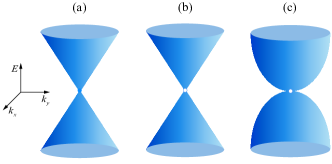
Figure 1: (color online) Schematic diagrams of three types of gapless SDCs. (a) Linear SDC in TIs, the Dirac node (a Kramers degeneracy) denoted by a solid dot is enforced by TRS. (b) and (c) are respectively the linear and quadratic nodelss SDCs in the opposite-parity and same-parity DSMs. The open circles in (b) and (c) represent the absence of Dirac node.

Recently, a remarkable experiment reported the observation of 2D gapless SDCs in some iron-based superconducting compounds with 3D bulk Dirac nodes protected by $C_{4z}$ rotation symmetry Zhang et al. (2019). Notably, the 2D gapless Dirac cones are located on the surface where the projections of the bulk Dirac nodes overlap, revealing that the largely-overlooked top and bottom surfaces perpendicular to the rotation axis also carry interesting topological surface states in DSMs. Inspired by this experiment, we consider two representative types of 3D DSMs protected by $C_{4z}$ rotation symmetry and explore the topological surface states on the top and bottom surfaces. Remarkably, we find that the gapless Dirac cones found on these surfaces display a number of features sharply distinct from the SDCs in TIs. The most evident difference is the absence of Dirac node in them, as illustrated in Fig.1. The spin textures of these nodeless SDCs are found to have a unique two-phase-angle dependence enforced by a subchiral symmetry, rather different from the one-phase-angle dependence exhibited in TIs. Furthermore, despite the absence of Dirac node, we find that the SDCs are also characterized by quantized $\pi$ Berry phases, even though one type of the SDCs has a quadratic dispersion. In the presence of TRS-breaking fields, we find that the responses of the surface and bulk Dirac cones display an interesting bulk-surface correspondence.

Linear nodeless SDCs in the opposite-parity DSM.— DSMs are materials whose conduction and valence bands cross at some isolated points (Dirac nodes) in the Brillouin zone Young et al. (2012); Wang et al. (2012, 2013); Liu et al. (2014a, b); Borisenko et al. (2014); Neupane et al. (2014). Depending on whether the band crossings occur between bands with opposite parity or same parity, DSMs can be roughly divided into two classes Qin et al. (2019). For the convenience of discussion, we dub the class involving bands with opposite (same) parity as opposite-parity (same-parity) DSMs.

Let us first consider the opposite-parity DSM. Focusing on a cubic-lattice realization, the minimal model is given by Wang et al. (2013); Yang and Nagaosa (2014)

$$\mathcal{H}(\boldsymbol{k}) = (m-t\cos k_{x}-t\cos k_{y}-t_{z}\cos k_{z})\sigma_{z}s_{0}$$ (1)

$$+\lambda(\sin k_{x}\sigma_{x}s_{z}-\sin k_{y}\sigma_{y}s_{0})$$

$$+\eta_{1}(\boldsymbol{k}_{s})\sin k_{z}\sigma_{x}s_{x}+\eta_{2}(\boldsymbol{k}_{s})\sin k_{z}\sigma_{x}s_{y},$$

where $\boldsymbol{k}_{s}=(k_{x},k_{y})$ denotes the $xy$-plane momentum, $\eta_{1}(\boldsymbol{k}_{s})=\eta_{1}(\cos k_{x}-\cos k_{y})$, $\eta_{2}(\boldsymbol{k}_{s})=\eta_{2}\sin k_{x}\sin k_{y}$, $\sigma_{i}$ and $s_{i}$ are Pauli matrices in orbital and spin space, and $\sigma_{0}$ and $s_{0}$ are the corresponding identity matrices. For notational simplicity, the lattice constants are set to unity throughout.

The Hamiltonian (1) has TRS ($\mathcal{T}=i\sigma_{0}s_{y}\mathcal{K}$) and inversion symmetry ($\mathcal{P}=\sigma_{z}s_{0}$), which ensures the band structure to be doubly degenerate everywhere. The additional existence of a $\mathcal{C}_{4z}$ rotation symmetry ($\mathcal{C}_{4z}=e^{i\frac{\pi}{4}(\sigma_{z}-2\sigma_{0})s_{z}}$) allows the presence of stable Dirac nodes of four-fold degeneracy on the two rotationally invariant $k_{z}$ axes in the Brillouin zone. Without loss of generality, below we consider all parameters in Eq.(1) to be positive, and $|m-2t|<t_{z}<m$. Accordingly, a band inversion occurs at the time-reversal invariant momentum $\boldsymbol{\Gamma}=(0,0,0)$, and there are two Dirac nodes located at $\boldsymbol{k}_{D,\pm}=\pm(0,0,k_{D})$ with $k_{D}=\arccos(m-2t)/t_{z}$. It is noteworthy that the existence and the locations of the bulk Dirac nodes do not depend on the two $\eta$ terms. However, as we shall show below, the $\eta$ terms have rather remarkable effects on the topological surface states.

When $\eta_{1}$ and $\eta_{2}$ vanish, the Hamiltonian (1) at a given $k_{z}$ is characterized by a $Z_{2}$ invariant Bernevig et al. (2006), and describes a 2D TI for $|k_{z}|<|\boldsymbol{k}_{D}|$, and a normal insulator for $|k_{z}|>|\boldsymbol{k}_{D}|$. For this situation, the DSM can be regarded as a stacking of 2D TIs in the $z$ direction. Accordingly, the surface states only exist on the side surfaces, and the iso-energy contours of these surface states form the so-called Fermi arcs. Once $\eta_{1}$ and $\eta_{2}$ become finite, the dispersions of the surface states on the side surfaces change dramatically Kargarian et al. (2016); Yan et al. (2020); Kargarian et al. (2018); Le et al. (2018); Qin et al. (2023), leading to the change of the Fermi-arc connectivity and the arising of SDCs that can have nontrivial interplay with superconductivity Kobayashi and Sato (2015); Kheirkhah et al. (2022); Wu and Wang (2022). Furthermore, it has been recognized that the $\eta$ terms can also give arise to gapless hinge states Szabó et al. (2020), a hallmark of second-order topology. These findings have one after another deepened our understanding on the bulk-boundary correspondence of DSMs. Now we show that our understanding remains incomplete.

To intuitively show that 2D gapless Dirac cones also exist on the top and bottom surfaces, we first introduce a set of momentum-dependent Pauli matrices, namely,

$$\tilde{s}_{x} = \cos\theta_{\boldsymbol{k}_{s}}s_{x}+\sin\theta_{\boldsymbol{k}_{s}}s_{y},$$

$$\tilde{s}_{y} = -\sin\theta_{\boldsymbol{k}_{s}}s_{x}+\cos\theta_{\boldsymbol{k}_{s}}s_{y},$$

$$\tilde{s}_{z} = s_{z},$$ (2)

where $\theta_{\boldsymbol{k}_{s}}=\arg[\eta_{1}(\boldsymbol{k}_{s})+i\eta_{2}(\boldsymbol{k}_{s})]$. In this work, two phase angles will be involved, one is $\theta_{\boldsymbol{k}_{s}}$, and the other is $\phi_{\boldsymbol{k}_{s}}=\arg(\sin k_{x}+i\sin k_{y})$. When considering the continuum counterpart of the lattice Hamiltonian, these two phase angles are implicitly assumed to take the corresponding continuum forms ( e.g., $\phi_{\boldsymbol{k}_{s}}=\arg(k_{x}+ik_{y})$).

It is easy to verify that this set of Pauli matrices also satisfies $[\tilde{s}_{i},\tilde{s}_{j}]=2i\epsilon_{ijk}\tilde{s}_{k}$ and $\{\tilde{s}_{i},\tilde{s}_{j}\}=2\delta_{ij}s_{0}$ for $i,j\in\{x,y,z\}$. Using them, the Hamiltonian can be rewritten as

$$\mathcal{H}(\boldsymbol{k}) = (m-t\cos k_{x}-t\cos k_{y}-t_{z}\cos k_{z})\sigma_{z}s_{0}$$ (3)

$$\lambda(\sin k_{x}\sigma_{x}\tilde{s}_{z}-\sin k_{y}\sigma_{y}s_{0})$$

$$+\eta(\boldsymbol{k}_{s})\sin k_{z}\sigma_{x}\tilde{s}_{x},$$

where $\eta(\boldsymbol{k}_{s})=\sqrt{\eta_{1}^{2}(\boldsymbol{k}_{s})+\eta_{2}^{2}(\boldsymbol{k}_{s})}$. The above form resembles the minimal model for 3D TIs Zhang et al. (2009), revealing the existence of gapless Dirac cones on the $z$-normal surfaces if $\eta(\boldsymbol{k}_{s})$ is nonzero. In this form, it is also easy to see that there exists a unitary operator anticommuting with the Hamiltonian, i.e., $\{\mathcal{C},\mathcal{H}\}=0$, with $\mathcal{C}=\sigma_{x}\tilde{s}_{y}$. Conventionally, such an anticommutation relation suggests that the Hamiltonian has chiral symmetry. However, here is not the case, simply because the operator $\mathcal{C}$ is not a constant operator but depends on partial components of the momentum vector. Such an algebraic property was recently discussed and dubbed subchiral symmetry in Ref.Mo et al. (2023). An important conclusion from Ref.Mo et al. (2023) is that the subchiral symmetry operator itself admits topological characterization, and its topological property will impart into the spin texture of the topological boundary states. Apparently, here $\tilde{s}_{y}$ displays a nontrivial winding as $\boldsymbol{k}_{s}$ goes around the origin once, indicating the nontrivialness of the subchiral symmetry operator.

Now let us proceed to derive the low-energy Hamiltonians describing the gapless Dirac cones on the $z$-normal surfaces. The methods are well developed Shen (2013). As usual, the first step is to do a low-energy expansion of the bulk Hamiltonian around the band-inversion momentum and decompose the Hamiltonian into two parts Yan et al. (2018), i.e., $\mathcal{H}=\mathcal{H}_{0}+\mathcal{H}_{1}$, with (see more details in the Supplemental Material sup )

$$\mathcal{H}_{0}(\boldsymbol{k}) = [M(\boldsymbol{k}_{s})+\frac{t_{z}}{2}k_{z}^{2}]\sigma_{z}s_{0}+\gamma(\boldsymbol{k}_{s})k_{z}\sigma_{x}\tilde{s}_{x},$$

$$\mathcal{H}_{1}(\boldsymbol{k}) = \lambda(k_{x}\sigma_{x}\tilde{s}_{z}-k_{y}\sigma_{y}s_{0}),$$ (4)

where $M(\boldsymbol{k}_{s})=m-2t-t_{z}+t(k_{x}^{2}+k_{y}^{2})/2$, and $\gamma(\boldsymbol{k}_{s})=\frac{1}{2}\sqrt{\eta_{1}^{2}(k_{x}^{2}-k_{y}^{2})^{2}+4\eta_{2}^{2}k_{x}^{2}k_{y}^{2}}$. Considering a half-infinity system occupying $z\geq 0$ ($z\leq 0$), replacing $k_{z}\rightarrow-i\partial_{z}$, and solving the eigenvalue equation $\mathcal{H}_{0}(\boldsymbol{k}_{s},-i\partial_{z})\psi_{\alpha}(x,y,z)=0$ under the boundary conditions $\psi_{\alpha}(z=0)=0$ and $\psi_{\alpha}(z\rightarrow\infty)=0$ ($\psi_{\alpha}(z\rightarrow-\infty)=0$), one will obtain two solutions corresponding to the zero-energy boundary states at the bottom (top) surface. Their explicit forms read Yan and Wang (2016)

$$\psi_{\alpha}^{a}(x,y,z)=\mathcal{N}\sin(\kappa_{1}z)e^{-\kappa_{2}|z|}e^{i(k_{x}x+k_{y}y)}\chi_{\alpha}^{a},$$ (5)

where the superscript $a=\{t,b\}$ labels the top and bottom surfaces, $\kappa_{1}=\sqrt{-2t_{z}M(\boldsymbol{k}_{s})-\gamma^{2}(\boldsymbol{k}_{s})}/t_{z}$, $\kappa_{2}=\gamma(\boldsymbol{k}_{s})/t_{z}$, $\mathcal{N}$ is a normalization constant, $\chi_{\alpha}^{t}$ satisfy $\sigma_{y}\tilde{s}_{x}\chi_{\alpha}^{t}=\chi_{\alpha}^{t}$, and $\chi_{\alpha}^{b}$ satisfy $\sigma_{y}\tilde{s}_{x}\chi_{\alpha}^{b}=-\chi_{\alpha}^{b}$. The normalizability of the wave functions determines the region hosting boundary states, which turns out to be the region bounded by the projection of the band-inversion surface, i.e., $M(\boldsymbol{k}_{s})<0$. Noteworthily, the point $\boldsymbol{k}_{s}=\mathbf{0}$, however, needs to be excluded since $\gamma(\boldsymbol{k}_{s})$ vanishes at this point. This result is consistent with the fact that the effective 1D Hamiltonian $\mathcal{H}(0,0,k_{z})$ is gapless, and the projections of the two bulk Dirac nodes are exactly located at this surface time-reversal invariant momentum Wang et al. (2013).

The low-energy Hamiltonians for the top and bottom surfaces are obtained by projecting $\mathcal{H}_{1}(\boldsymbol{k})$ onto the Hilbert space spanned by the corresponding two zero-energy eigenstates. Since $[\sigma_{y}\tilde{s}_{x},\mathcal{C}]=0$, we can choose $\chi_{\alpha}^{t/b}$ to be the eigenstates of the subchiral symmetry operator. Without loss of generality, we choose $\chi_{\pm}^{t}=(|\sigma_{y}=1,\tilde{s}_{x}=1\rangle\pm|\sigma_{y}=-1,\tilde{s}_{x}=-1\rangle)/\sqrt{2}$, and $\chi_{\pm}^{b}=(|\sigma_{y}=1,\tilde{s}_{x}=-1\rangle\mp|\sigma_{y}=-1,\tilde{s}_{x}=1\rangle)/\sqrt{2}$, so that $\mathcal{C}\chi_{\pm}^{t/b}=\pm\chi_{\pm}^{t/b}$. Here $|\sigma_{y}=\pm 1,\tilde{s}_{x}=\pm 1\rangle$ stands for $|\sigma_{y}=\pm 1\rangle\otimes|\tilde{s}_{x}=\pm 1\rangle$, with $\sigma_{y}|\sigma_{y}=\pm 1\rangle=\pm|\sigma_{y}=\pm 1\rangle$ and $\tilde{s}_{x}|\tilde{s}_{x}=\pm 1\rangle=\pm|\tilde{s}_{x}=\pm 1\rangle$. Accordingly, in the basis of $(\psi_{-}^{t},\psi_{+}^{t})^{T}$ or $(\psi_{+}^{b},\psi_{-}^{b})^{T}$, the low-energy surface Hamiltonians are found to take the form

$$\mathcal{H}_{t/b}(\boldsymbol{k}_{s})=\lambda(k_{x}\rho_{y}-k_{y}\rho_{x}),$$ (6)

where $\rho_{i}$ denote Pauli matrices acting on the two eigenstates of the subchiral symmetry operator. Apparently, the surface Hamiltonians take the exactly same form as in TIs Zhang et al. (2009). However, here the linearly dispersive SDCs have two fundamental differences. First, as discussed above, surface states are absent at $\boldsymbol{k}_{s}=\mathbf{0}$. This fact indicates the absence of Dirac node in this class of SDCs. Second, here the basis functions are the eigenstates of the subchiral symmetry operator, which themselves carry nontrivial topological properties as the subchiral symmetry operator displays a nontrivial winding with respect to the momentum. As will be shown below, this property has nontrivial effects on the spin texture and Berry phase.

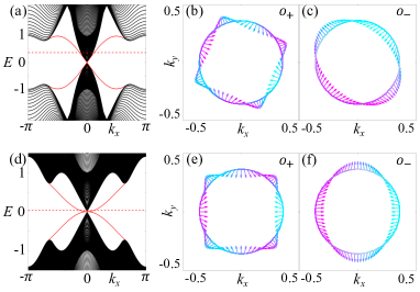
Figure 2: (color online) Energy spectra at $k_{y}=0$ for a sample with open (periodic) boundary conditions in the $z$ ($x$ and $y$) direction and spin textures of the top-surface Dirac cones. The solid red lines in (a) and (d) show the existence of linear and quadratic SDCs in the opposite-parity and same-parity DSMs, respectively. The orbital-resolved spin textures in (b) and (c) [(e) and (f)] are plotted on the iso-energy contour of the SDC illustrated by the red dashed line corresponding to $E=0.375$ ($0.038$) in (a) [(d)]. Common parameters are $m=3$, $t=t_{z}=2$, $\lambda=1$. $\eta_{1}=\eta_{2}=5$ in (a)-(c), and $\eta_{1}=\eta_{2}=0.5$ in (d)-(f).

To determine the spin texture and Berry phase, we need to first determine the spinor part of the wave functions for the SDCs. To be specific, let us focus on the upper band of the top-surface Dirac cone for a detailed discussion (the spin texture for the bottom-surface Dirac cone is just opposite, and the Berry phase is same). According to the form of $\mathcal{H}_{t}$ in Eq.(6), it is easy to find that the eigenstate for the upper band is $(1,ie^{i\phi_{\boldsymbol{k}_{s}}})^{T}/\sqrt{2}$. By further taking into account the nontrivial basis functions, the corresponding spinor takes the form

$$|u(\boldsymbol{k}_{s})\rangle=\frac{1}{\sqrt{2}}(\chi_{-}^{t}+ie^{i\phi_{\boldsymbol{k}_{s}}}\chi_{+}^{t}).$$ (7)

Because the spin and orbital are entangled by spin-orbit coupling, we consider the orbital-resolved spin textureCao et al. (2013); Park et al. (2012); Zhang et al. (2013), which are given by $\bar{s}_{i}^{(o_{\pm})}(\boldsymbol{k}_{s})=\langle u(\boldsymbol{k}_{s})|(\sigma_{0}\pm\sigma_{z})s_{i}|u(\boldsymbol{k}_{s})\rangle/2$, where the two superscripts $o_{+}$ and $o_{-}$ label the two orbitals (here we ignore the constant factor $\hbar/2$ connecting the Pauli matrices to the spin operators). A straightforward calculation obtains

$$\bar{s}_{x}^{(o_{\pm})}(\boldsymbol{k}_{s}) = \pm[\sin(\theta_{\boldsymbol{k}_{s}}\mp\phi_{\boldsymbol{k}_{s}})]/2,$$

$$\bar{s}_{y}^{(o_{\pm})}(\boldsymbol{k}_{s}) = \mp[\cos(\theta_{\boldsymbol{k}_{s}}\mp\phi_{\boldsymbol{k}_{s}})]/2,$$

$$\bar{s}_{z}^{(o_{\pm})}(\boldsymbol{k}_{s}) = 0.$$ (8)

The spin polarizations are aligned in the surface plane. This is similar to the spin textures of the SDCs in TIs. However, here a striking difference is that the spin textures depend on two phase angles rather than one as in TIs Zhang et al. (2013). Particularly, the angle $\theta_{\boldsymbol{k}_{s}}$ originates from the subchiral symmetry, and will change $4\pi$ when the polar angle of the surface momentum changes $2\pi$. Due to the unique two-phase-angle dependence, the two orbital-resolved spin textures display a remarkable property, namely, their spin polarizations wind one and three times respectively when $\boldsymbol{k}_{s}$ winds the origin once, as shown in Figs.2(a)-(c). This is rather different from the TI for which only one time of winding will exhibit Hasan and Kane (2010); Qi and Zhang (2011).

Also based on $|u(\boldsymbol{k}_{s})\rangle$, the Berry connection is given by Xiao et al. (2010)

$$A_{\alpha}(\boldsymbol{k}_{s})=-i\langle u(\boldsymbol{k}_{s})|\partial_{k_{\alpha}}u(\boldsymbol{k}_{s})\rangle=\frac{1}{2}\partial_{k_{\alpha}}(\theta_{\boldsymbol{k}_{s}}+\phi_{\boldsymbol{k}_{s}}),$$ (9)

where $\alpha=\{x,y\}$. Since $\theta_{\boldsymbol{k}_{s}}$ will wind $4\pi$ and $\phi_{\boldsymbol{k}_{s}}$ will wind $2\pi$ when $\boldsymbol{k}_{s}$ winds $2\pi$, it indicates that one particle will accumulate a $\pi$ (mod $2\pi$) Berry phase when it goes around the surface Fermi loop once. This important result indicates that the quantized $\pi$ Berry phase remains intact even though the singular Dirac node is absent in the SDCs.

Quadratic nodeless SDCs in the same-parity DSM.—Let us move our attention to the same-parity DSM. Also focusing on a cubic-lattice realization, the minimal model is given by Yang and Nagaosa (2014)

$$\mathcal{H}(\boldsymbol{k}) = (m-t\cos k_{x}-t\cos k_{y}-t_{z}\cos k_{z})\sigma_{z}s_{0}$$ (10)

$$\lambda\sin k_{z}(\sin k_{x}\sigma_{x}s_{0}-\sin k_{y}\sigma_{y}s_{z})$$

$$+\eta_{1}(\boldsymbol{k}_{s})\sigma_{y}s_{x}+\eta_{2}(\boldsymbol{k}_{s})\sigma_{y}s_{y}.$$

Without loss of generality, below we again consider all parameters to be positive, and $|m-2t|<t_{z}<m$ so that the two bulk Dirac nodes are also located at $\boldsymbol{k}_{D,\pm}$. Similar to the first model, this model also supports interesting gapless topological states on the side surfaces and hinges Szabó et al. (2020). However, much less is known about the top and bottom surfaces. Below we explore the surface states on these two surfaces.

The first thing to note is that the Hamiltonian (10) also has a subchiral symmetry, with the symmetry operator given by

$$\tilde{\mathcal{C}}=\sin\phi_{\boldsymbol{k}_{s}}\sigma_{x}s_{0}+\cos\phi_{\boldsymbol{k}_{s}}\sigma_{y}s_{z}.$$ (11)

Also using the continuum-model approach, we find that the wave functions of surface states on the top and bottom surfaces are given by

$$\tilde{\psi}_{\alpha}^{a}(x,y,z)=\tilde{\mathcal{N}}\sin(\tilde{\kappa}_{1}z)e^{-\tilde{\kappa}_{2}|z|}e^{i(k_{x}x+k_{y}y)}\tilde{\chi}_{\alpha}^{a},$$ (12)

where $\tilde{\kappa}_{1}=\sqrt{-2t_{z}M(\boldsymbol{k}_{s})-\lambda^{2}\boldsymbol{k}_{s}^{2}}/t_{z}$, $\tilde{\kappa}_{2}=\lambda|\boldsymbol{k}_{s}|/t_{z}$, and $\tilde{\chi}_{\alpha}^{a}$ satisfy $\tilde{\mathcal{C}}\tilde{\chi}_{\alpha}^{a}=\alpha\tilde{\chi}_{\alpha}^{a}$ with $\alpha=\pm$. The normalizability of the wave functions also suggests that the region hosting surface states corresponds to $M(\boldsymbol{k}_{s})<0$ but with the point $\boldsymbol{k}_{s}=\mathbf{0}$ excluded. Without loss of generality, we choose $\tilde{\chi}_{\pm}^{t}=|\sigma_{\pm}=\pm 1,s_{z}=\pm 1\rangle$, and $\tilde{\chi}_{\mp}^{b}=|\sigma_{\pm}=\mp 1,s_{z}=\pm 1\rangle$, where $\sigma_{\pm}=\sin\phi_{\boldsymbol{k}_{s}}\sigma_{x}\pm\cos\phi_{\boldsymbol{k}_{s}}\sigma_{y}$. In the basis of $(\tilde{\psi}_{+}^{t},\tilde{\psi}_{-}^{t})^{T}$ or $(\tilde{\psi}_{-}^{b},\tilde{\psi}_{+}^{b})^{T}$, the low-energy surface Hamiltonians are found to take the form

$$\mathcal{H}_{t/b}(\boldsymbol{k}_{s})=\pm\left(\begin{array}[]{cc}0&\eta_{-}(\boldsymbol{k}_{s})e^{i\phi_{\boldsymbol{k}_{s}}}\\ \eta_{+}(\boldsymbol{k}_{s})e^{-i\phi_{\boldsymbol{k}_{s}}}&0\\ \end{array}\right),$$ (15)

where $+$ ($-$) refers to the top (bottom) surface, and $\eta_{\pm}(\boldsymbol{k}_{s})=-\frac{\eta_{1}}{2}(k_{x}^{2}-k_{y}^{2})\pm i\eta_{2}k_{x}k_{y}$. It is easy to see that the energy dispersions of the surface Hamiltonian are given by $E_{\pm}(\boldsymbol{k}_{s})=\pm\sqrt{\eta_{+}(\boldsymbol{k}_{s})\eta_{-}(\boldsymbol{k}_{s})}$, which are quadratic rather than linear, as shown in Fig.2(d). It is worth emphasizing that the Dirac node is also absent for this class of quadratic SDCs.

Again let us focus on the upper band of the top-surface Dirac cone for a discussion of its spin texture and Berry phase. The corresponding spinor part of the wave function is found to take the form

$$|\tilde{u}(\boldsymbol{k}_{s})\rangle=\frac{1}{\sqrt{2}}(\tilde{\chi}_{+}^{t}+e^{i(\theta_{\boldsymbol{k}_{s}}-\phi_{\boldsymbol{k}_{s}})}\tilde{\chi}_{-}^{t}).$$ (16)

Based on $|\tilde{u}(\boldsymbol{k}_{s})\rangle$, one finds

$$\bar{s}_{x}^{(o_{\pm})}(\boldsymbol{k}_{s}) = [\cos(\theta_{\boldsymbol{k}_{s}}\mp\phi_{\boldsymbol{k}_{s}})]/2,$$

$$\bar{s}_{y}^{(o_{\pm})}(\boldsymbol{k}_{s}) = [\sin(\theta_{\boldsymbol{k}_{s}}\mp\phi_{\boldsymbol{k}_{s}})]/2,$$

$$\bar{s}_{z}^{(o_{\pm})}(\boldsymbol{k}_{s}) = 0.$$ (17)

The two orbital-resolved spin textures also depend on two phase angles and display different windings, as shown in Figs.2(e) and 2(f). The Berry connection is given by

$$A_{\alpha}(\boldsymbol{k}_{s}) = -i\langle\tilde{u}(\boldsymbol{k}_{s})|\partial_{k_{\alpha}}\tilde{u}(\boldsymbol{k}_{s})\rangle=\frac{1}{2}\partial_{k_{\alpha}}(\theta_{\boldsymbol{k}_{s}}-\phi_{\boldsymbol{k}_{s}}).\,$$ (18)

Similarly, this result indicates that the particle will accumulate a $\pi$ (mod $2\pi$) Berry phase when it goes around the surface Fermi loop once. This is a remarkable result since usually a quadratic cone is accompanied with a zero (mod $2\pi$) Berry phase Novoselov et al. (2006). From Eq.(18), it is apparent that the $\pi$ Berry phase is attributed to $\phi_{\boldsymbol{k}_{s}}$, indicating its origin from the subchiral symmetry rather than the quadratic band structure.

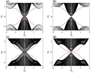
Figure 3: (Color online) Energy spectra at $k_{y}=0$ for a sample with open boundary conditions only in the $z$ direction (lattice sites $N_{z}=400$). Common parameters are $m=4$, $t=t_{z}=2$, and $\lambda=1$. The values of $(\eta_{1},\eta_{2},B_{1},B_{2})$ in (a), (b), (c) and (d) are $(5,5,0.2,0)$, $(5,5,0,0.2)$, $(1,1,0.2,0)$, and $(1,1,0,0.2)$, respectively. (a) and (b) correspond to the opposite-parity DSM, and (c) and (d) refer to the same-parity DSM.

Response to TRS-breaking fields.—It is known that the SDCs in TIs are protected by TRS, and the lift of TRS can gap the SDCs Qi et al. (2008); Chen et al. (2010b). On the other hand, it is known that TRS-breaking fields will split one bulk Dirac node into two Weyl nodes Armitage et al. (2018). Here the SDCs are nodeless, and therefore are not protected by TRS. To open a gap to the SDCs, mathematically a Dirac mass term of the form $m_{D}\rho_{z}$ is required to enter into the surface Hamiltonian (6) or (15). As the basis functions for the surface Hamiltonians are eigenstates of the subchiral symmetry operators, a necessary but not sufficient condition to generate the Dirac mass term is that the TRS-breaking fields must commute with the subchiral symmetry operator. To demonstrate the above arguments, we consider two types of Zeeman splitting fields, i.e., $B_{1}\sigma_{0}s_{z}$ and $B_{2}\sigma_{z}s_{z}$. For the opposite-parity DSM, $B_{1}\sigma_{0}s_{z}$ preserves the subchiral symmetry, while $B_{2}\sigma_{z}s_{z}$ does not. The situation is just the opposite for the same-parity DSM. As shown in Fig.3, the results show that $B_{2}\sigma_{z}s_{z}$ gaps the SDCs in the opposite-parity DSM, while $B_{1}\sigma_{0}s_{z}$ gaps the SDCs in the same-parity DSM, in consistent with the above analysis. Interestingly, we note no matter whether the SDCs are gapped or not, the surface states are always connected with the bulk nodes, either at $E=0$ or $\pm B_{1}$ ($\pm B_{2}$), which can be viewed as a kind of bulk-surface correspondence. Furthermore, for the gapless cases shown in Figs.3(a) and 3(d), we note that the Zeeman fields flatten the SDCs, which may have nontrivial interplay with interactions.

Discussions and conclusions.— We have unveiled the existence of two types of nodeless SDCs with linear and quadratic dispersion, quantized $\pi$ Berry phases and unconventional spin textures, expanding our understanding of the topological surface states and bulk-boundary correspondence in DSMs. Our predictions are of general relevance as our theory is based on two generic classes of DSMs. In experiments, the dispersion of the SDCs and the concomitant unconventional spin textures can be directly detected by using spin-resolved and angle-resolved photoemission spectroscopy Zhang et al. (2019); Souma et al. (2011); Wang et al. (2011); Lv et al. (2015); Xu et al. (2016); Sakano et al. (2020); Dai et al. (2021). To conclude, our findings enrich the types of SDCs with fascinating properties, opening directions for future studies of Dirac physics.

Acknowledgements.—We would like to thank Zhigang Wu for helpful discussions and insightful comments. This work is supported by the National Natural Science Foundation of China (Grant No.12174455) and the Natural Science Foundation of Guangdong Province (Grant No. 2021B1515020026).

The supplemental material contains two sections. In the first section, we provide the derivation details of the low-energy surface Hamiltonians, spin textures, and Berry phases for the opposite-parity Dirac semimetal. In the second section, we derive the orbital-resolved spin textures associated with the surface Dirac cone in a topological insulator to highlight the difference of the surface Dirac cones in Dirac semimetals and topological insulators.

I I. The low-energy surface Hamiltonians, spin textures, and Berry phases for the Dirac semimetals

Because the derivation steps are rather similar for the two representative types of Dirac semimetals, here we restrict ourselves to the opposite-parity Dirac semimetal for a detailed discussion. We start from the tight-binding Hamiltonian describing the opposite-parity Dirac semimetal,

$$\mathcal{H}(\boldsymbol{k}) = (m-t\cos k_{x}-t\cos k_{y}-t_{z}\cos k_{z})\sigma_{z}s_{0}+\lambda(\sin k_{x}\sigma_{x}s_{z}-\sin k_{y}\sigma_{y}s_{0})$$ (S1)

$$+\eta_{1}(\cos k_{x}-\cos k_{y})\sin k_{z}\sigma_{x}s_{x}+\eta_{2}\sin k_{x}\sin k_{y}\sin k_{z}\sigma_{x}s_{y},$$

where $\sigma_{i}$ and $s_{i}$ are Pauli matrices respectively acting on orbital and spin degrees of freedom, and $\sigma_{0}$ and $s_{0}$ are the corresponding $2\times 2$ identity matrices. For notational simplicity, the lattice constants are set to unity.

Without loss of generality, we consider that the band inversion occurs at the center of the bulk Brillouin zone, i.e., the time-reversal invariant momentum $\boldsymbol{\Gamma}=(0,0,0)$, so that the bulk Dirac points are located on the $k_{z}$ axis going through $\boldsymbol{\Gamma}$. Because the surface states originate from the band inversion, we expand the tight-binding Hamiltonian around the band inversion momentum and obtain the continuum Hamiltonian to derive the low-energy Hamiltonians describing the surface states. For each term in the Hamiltonian, we only keep the leading-order momentum terms to simplify the analytical derivation. Accordingly, the continuum Hamiltonian is given by

$$\mathcal{H}(\boldsymbol{k}) = [M(\boldsymbol{k}_{s})+\frac{t_{z}}{2}k_{z}^{2}]\sigma_{z}s_{0}+\lambda(k_{x}\sigma_{x}s_{z}-k_{y}\sigma_{y}s_{0})$$ (S2)

$$-\frac{\eta_{1}}{2}(k_{x}^{2}-k_{y}^{2})k_{z}\sigma_{x}s_{x}+\eta_{2}k_{x}k_{y}k_{z}\sigma_{x}s_{y},$$

where $\boldsymbol{k}_{s}=(k_{x},k_{y})$ denotes the momentum vector parallel to the $z$-normal surfaces, and $M(\boldsymbol{k}_{s})=m-2t-t_{z}+t(k_{x}^{2}+k_{y}^{2})/2$. Next, we define a new set of Pauli matrices of the form

$$\tilde{s}_{x}=\cos\theta_{\boldsymbol{k}_{s}}s_{x}+\sin\theta_{\boldsymbol{k}_{s}}s_{y},$$

$$\tilde{s}_{y}=-\sin\theta_{\boldsymbol{k}_{s}}s_{x}+\cos\theta_{\boldsymbol{k}_{s}}s_{y},$$

$$\tilde{s}_{z}=s_{z},$$ (S3)

where $\theta_{\boldsymbol{k}_{s}}=\arg[-\frac{\eta_{1}}{2}(k_{x}^{2}-k_{y}^{2})+i\eta_{2}k_{x}k_{y}]$, which is well defined except at $\boldsymbol{k}_{s}=\mathbf{0}$. It is easy to check that the new set of Pauli matrices $\tilde{s}_{i}$ satisfies the algebraic properties associated with the conventional Pauli matrices, i.e., $[\tilde{s}_{i},\tilde{s}_{j}]=2i\epsilon_{ijk}\tilde{s}_{k}$ and $\{\tilde{s}_{i},\tilde{s}_{j}\}=2\delta_{ij}s_{0}$ for $i,j\in\{x,y,z\}$. Using this new set of Pauli matrices, the continuum Hamiltonian can be rewritten as

$$\mathcal{H}(\boldsymbol{k})=[M(\boldsymbol{k}_{s})+\frac{t_{z}}{2}k_{z}^{2}]\sigma_{z}s_{0}+\lambda(k_{x}\sigma_{x}\tilde{s}_{z}-k_{y}\sigma_{y}s_{0})+\gamma(\boldsymbol{k}_{s})k_{z}\sigma_{x}\tilde{s}_{x},$$ (S4)

where $\gamma(\boldsymbol{k}_{s})=\frac{1}{2}\sqrt{\eta_{1}^{2}(k_{x}^{2}-k_{y}^{2})^{2}+4\eta_{2}^{2}k_{x}^{2}k_{y}^{2}}$. In this form, it is easy to find that the Hamiltonian anticommutes with the operator $\mathcal{C}=\sigma_{x}\tilde{s}_{y}$. Conventionally, when there exists a momentum-independent unitary operator anticommuting with the Hamiltonian, it implies that the Hamiltonian has chiral symmetry. The momentum independence is because the chiral symmetry is a non-spatial symmetry. However, here the operator $\mathcal{C}$ depends on momentum, thereby the anticommutation relation between $\mathcal{C}$ and $\mathcal{H}(\boldsymbol{k})$ does not suggest the existence of the chiral symmetry. Nevertheless, here $\mathcal{C}$ only depends on $k_{x}$ and $k_{y}$. For situations where $k_{x}$ and $k_{y}$ are good quantum numbers and can be viewed as a parameter, such as the surface states on the $z$-normal surfaces considered below, this anticommutation relation has the conventional meaning of chiral symmetry. In Ref.Mo et al. (2023), the authors introduced the concept termed “subchiral symmetry” to describe the existence of such an anticommutation relation, and showed that the existence of subchiral symmetry can have nontrivial effects on the spin textures and Berry phases of the boundary states.

Now let us derive the low-energy Hamiltonians describing the surface states on the $z$-normal surface states. To simplify the derivation, we consider a half-infinity system to avoid the coupling between the surface states on the top and bottom surfaces. First, we assume that the system occupies the region with coordinates satisfying $z\geq 0$, accordingly the surface at $z=0$ corresponds to the bottom surface. Second, we decompose the continuum Hamiltonian into two parts Yan et al. (2018), i.e., $\mathcal{H}=\mathcal{H}_{0}+\mathcal{H}_{1}$, where

$$\mathcal{H}_{0}(\boldsymbol{k}) = [M(\boldsymbol{k}_{s})+\frac{t_{z}}{2}k_{z}^{2}]\sigma_{z}s_{0}+\gamma(\boldsymbol{k}_{s})k_{z}\sigma_{x}\tilde{s}_{x},$$

$$\mathcal{H}_{1}(\boldsymbol{k}) = \lambda(k_{x}\sigma_{x}\tilde{s}_{z}-k_{y}\sigma_{y}s_{0}).$$ (S5)

In the presence of a boundary in the $z$ direction, the translation symmetry is broken in the $z$ direction, and $k_{z}$ needs to be replaced by $-i\partial_{z}$. Accordingly,

$$\mathcal{H}_{0}(\boldsymbol{k}_{s},-i\partial_{z})=[M(\boldsymbol{k}_{s})-\frac{t_{z}}{2}\partial_{z}^{2}]\sigma_{z}s_{0}-i\gamma(\boldsymbol{k}_{s})\partial_{z}\sigma_{x}\tilde{s}_{x},$$ (S6)

and $\mathcal{H}_{1}$ retains its form as the translation symmetry converses in the $xy$ plane. The next step is to solve the eigenvalue equation

$$\mathcal{H}_{0}(\boldsymbol{k}_{s},-i\partial_{z})\psi(x,y,z)=E(\boldsymbol{k}_{s})\psi(x,y,z)$$ (S7)

under the boundary conditions $\psi(x,y,z=0)=\psi(x,y,z\rightarrow+\infty)=0$. We find that there are two zero-energy solutions satisfying the boundary conditions, and the solutions have the form

$$\psi_{\alpha}^{b}(x,y,z)=\mathcal{N}\sin(\kappa_{1}z)e^{-\kappa_{2}z}e^{i(k_{x}x+k_{y}y)}\chi_{\alpha}^{b},$$ (S8)

where $\alpha=\pm$, $\kappa_{1}=\sqrt{-2t_{z}M(\boldsymbol{k}_{s})-\gamma^{2}(\boldsymbol{k}_{s})}/t_{z}$, $\kappa_{2}=\gamma(\boldsymbol{k}_{s})/t_{z}$, $\mathcal{N}=2\sqrt{|\kappa_{2}(\kappa_{1}^{2}+\kappa_{2}^{2})/\kappa_{1}^{2}|}$ is the normalization constant, and $\chi_{\alpha}^{b}$ satisfy $\sigma_{y}\tilde{s}_{x}\chi_{\alpha}^{b}=-\chi_{\alpha}^{b}$. To be normalizable, the two parameters $\kappa_{1}$ and $\kappa_{2}$ in the wave functions need to satisfy the constraint that $\kappa_{1}^{2}+\kappa_{2}^{2}>0$ and $\kappa_{2}\neq 0$. Accordingly, one finds that the zero-energy surface states exist within the region $M(\boldsymbol{k}_{s})<0$ but with the special point $\boldsymbol{k}_{s}=\mathbf{0}$ excluded.

From the equation $\sigma_{y}\tilde{s}_{x}\chi_{\alpha}^{b}=-\chi_{\alpha}^{b}$, it is easy to see that the spinors $\chi_{\alpha}^{b}$ can be chosen as $|\sigma_{y}=1,\tilde{s}_{x}=-1\rangle$ and $|\sigma_{y}=-1,\tilde{s}_{x}=1\rangle$. However, as $\sigma_{y}\tilde{s}_{x}$ commutes with the subchiral symmetry operator $\mathcal{C}=\sigma_{x}\tilde{s}_{y}$, we choose $\chi_{\alpha}^{b}$ to be simultaneously the eigenstates of $\sigma_{y}\tilde{s}_{x}$ and $\sigma_{x}\tilde{s}_{y}$. Without loss of generality, we choose

$$\chi_{+}^{b} = \frac{1}{\sqrt{2}}(|\sigma_{y}=1,\tilde{s}_{x}=-1\rangle-|\sigma_{y}=-1,\tilde{s}_{x}=1\rangle),$$

$$\chi_{-}^{b} = \frac{1}{\sqrt{2}}(|\sigma_{y}=1,\tilde{s}_{x}=-1\rangle+|\sigma_{y}=-1,\tilde{s}_{x}=1\rangle).$$ (S9)

One can check $\mathcal{C}\chi_{\pm}^{b}=\pm\chi_{\pm}^{b}$. The low-energy Hamiltonian for the surface states is then obtained by projecting $\mathcal{H}_{1}$ onto the two-dimensional Hilbert space spanned by $\psi_{+}^{b}$ and $\psi_{-}^{b}$. To be specific, we choose the basis to be $(\psi_{+}^{b},\psi_{-}^{b})^{T}$, then the matrix elements of the low-energy surface Hamiltonian are given by

$$[\mathcal{H}_{b}(\boldsymbol{k}_{s})]_{11}=\int_{0}^{+\infty}[\psi_{+}^{b}(x,y,z)]^{{\dagger}}\mathcal{H}_{1}(\boldsymbol{k}_{s},-i\partial_{z})\psi_{+}^{b}(x,y,z)dz,$$

$$[\mathcal{H}_{b}(\boldsymbol{k}_{s})]_{12}=\int_{0}^{+\infty}[\psi_{+}^{b}(x,y,z)]^{{\dagger}}\mathcal{H}_{1}(\boldsymbol{k}_{s},-i\partial_{z})\psi_{-}^{b}(x,y,z)dz,$$

$$[\mathcal{H}_{b}(\boldsymbol{k}_{s})]_{21}=\int_{0}^{+\infty}[\psi_{-}^{b}(x,y,z)]^{{\dagger}}\mathcal{H}_{1}(\boldsymbol{k}_{s},-i\partial_{z})\psi_{+}^{b}(x,y,z)dz,$$

$$[\mathcal{H}_{b}(\boldsymbol{k}_{s})]_{22}=\int_{0}^{+\infty}[\psi_{-}^{b}(x,y,z)]^{{\dagger}}\mathcal{H}_{1}(\boldsymbol{k}_{s},-i\partial_{z})\psi_{-}^{b}(x,y,z)dz.$$ (S10)

Now $\boldsymbol{k}_{s}=(k_{x},k_{y})$ has the meaning of the momentum vector in the surface Brillouin zone. In the matrix form, one has

$$\mathcal{H}_{b}(\boldsymbol{k}_{s})=\lambda\left(\begin{array}[]{cc}0&-k_{y}-ik_{x}\\ -k_{y}+ik_{x}&0\\ \end{array}\right).$$ (S13)

In terms of Pauli matrices, the low-energy surface Hamiltonian can be rewritten in the form

$$\mathcal{H}_{b}(\boldsymbol{k}_{s})=\lambda(k_{x}\rho_{y}-k_{y}\rho_{x}),$$ (S14)

where $\rho_{i}$ denote Pauli matrices. Because the underlying basis functions are the eigenstates of the subchiral symmetry operator, one can see that the surface Hamiltonian takes an off-diagonal form. From this surface Hamiltonian, one obtains the energy spectra of the surface states, which read

$$E_{\pm}(\boldsymbol{k}_{s})=\pm\lambda\sqrt{k_{x}^{2}+k_{y}^{2}}=\pm\lambda|\boldsymbol{k}_{s}|.$$ (S15)

The energy spectra form a linear Dirac cone. However, since the surface states do not exist at $\boldsymbol{k}_{s}=\mathbf{0}$, this linear surface Dirac cone does not host the Dirac node occurring at this surface time-reversal invariant momentum, which is fundamentally different from the linear surface Dirac cone in topological insulators. The latter is known to host a time-reversal-symmetry-enforced Dirac node in its structure.

To obtain the low-energy Hamiltonian describing the surface states on the top surface, it is convenient to assume a half-infinity geometry with the region $z\leq 0$ occupied. Then the surface at $z=0$ corresponds to the top surface. Similarly, the next step is to solve the eigenvalue equation

$$\mathcal{H}_{0}(\boldsymbol{k}_{s},-i\partial_{z})\psi(x,y,z)=E(\boldsymbol{k}_{s})\psi(x,y,z),$$ (S16)

but with the boundary conditions modified as $\psi(x,y,z=0)=\psi(x,y,z\rightarrow-\infty)=0$. It is straightforward to find that there are also two zero-energy solutions satisfying the boundary conditions, and the solutions have a form similar to that in Eq.(S45). Namely, we have

$$\psi_{\alpha}^{t}(x,y,z)=\mathcal{N}\sin(\kappa_{1}z)e^{\kappa_{2}z}e^{i(k_{x}x+k_{y}y)}\chi_{\alpha}^{t}.$$ (S17)

Here the parameters $\kappa_{1}$, $\kappa_{2}$ and $\mathcal{N}$ are the same as before. The only difference is that now the spinors $\chi_{\alpha}^{t}$ satisfy the eigenvalue equation, $\sigma_{y}\tilde{s}_{x}\chi_{\alpha}^{t}=\chi_{\alpha}^{t}$. Two natural solutions are $|\sigma_{y}=1,\tilde{s}_{x}=1\rangle$ and $|\sigma_{y}=-1,\tilde{s}_{x}=-1\rangle$. However, since the subchiral symmetry operator commutes with $\sigma_{y}\tilde{s}_{x}$, again we choose the eigenstates to be simultaneously the eigenstates of $\sigma_{y}\tilde{s}_{x}$ and the subchiral symmetry operator. Concretely, we choose

$$\chi_{+}^{t} = \frac{1}{\sqrt{2}}(|\sigma_{y}=1,\tilde{s}_{x}=1\rangle+|\sigma_{y}=-1,\tilde{s}_{x}=-1\rangle),$$

$$\chi_{-}^{t} = \frac{1}{\sqrt{2}}(|\sigma_{y}=1,\tilde{s}_{x}=1\rangle-|\sigma_{y}=-1,\tilde{s}_{x}=-1\rangle).$$ (S18)

It is easy to check that $\mathcal{C}\chi_{\pm}^{t}=\pm\chi_{\pm}^{t}$. Choose the basis to be $(\psi_{-}^{t},\psi_{+}^{t})^{T}$ and project $\mathcal{H}_{1}$ onto it, we obtain the low-energy surface Hamiltonian for the top surface, which takes the exactly same form as Eq.(S14), i.e.,

$$\mathcal{H}_{t}(\boldsymbol{k}_{s})=\lambda(k_{x}\rho_{y}-k_{y}\rho_{x}).$$ (S19)

Despite the same form, one needs to note that here the basis is different. Eqs.(S14) and (S19) give the Eq.(6) in the main article.

In the following, let us derive the spin textures associated with the surface states. Without loss of generality, we focus on the upper-half cone. We first consider the bottom surface. According to the low-energy surface Hamiltonian in Eq.(S14), one knows that the eigenstate for the upper band is of the simple form $(1,ie^{i\phi_{\boldsymbol{k}_{s}}})^{T}/\sqrt{2}$, where $\phi_{\boldsymbol{k}_{s}}=\text{arg}(k_{x}+ik_{y})$. However, here the basis is not the usual spin-up and spin-down basis, thereby one has to take into account the basis functions to determine the spin textures correctly. In addition, since both the spin texture and the Berry phase are determined by the spinor part of the wave function, we can ignore the space dependence and just focus on the spinor part describing the internal degrees of freedom. By taking into account the basis functions, the spinor for the upper band of the surface states on the bottom surface is given by

$$|u^{b}(\boldsymbol{k}_{s})\rangle=\frac{1}{\sqrt{2}}(\chi_{+}^{b}+ie^{i\phi_{\boldsymbol{k}_{s}}}\chi_{-}^{b}).$$ (S20)

Because the spin and orbital are strongly coupled by spin-orbit coupling, we should consider the orbital-resolved spin textures, which are given by

$$\bar{s}_{i}^{b,o_{\pm}}(\boldsymbol{k}_{s})=\langle u^{b}(\boldsymbol{k}_{s})|\frac{(\sigma_{0}\pm\sigma_{z})}{2}s_{i}|u^{b}(\boldsymbol{k}_{s})\rangle.$$ (S21)

where the two superscripts $o_{+}$ and $o_{-}$ label the two orbitals (here we ignore the constant factor $\hbar/2$ connecting the Pauli matrices to the spin operators).

Before proceeding, it is worth noting that since $\tilde{s}_{x}=\cos\theta_{\boldsymbol{k}_{s}}s_{x}+\sin\theta_{\boldsymbol{k}_{s}}s_{y}$, the explicit expressions of the two eigenstates of $\tilde{s}_{x}$ are

$$|\tilde{s}_{x}=1\rangle=\frac{1}{\sqrt{2}}\left(\begin{array}[]{c}1\\ e^{i\theta_{\boldsymbol{k}_{s}}}\\ \end{array}\right),\quad|\tilde{s}_{x}=-1\rangle=\frac{1}{\sqrt{2}}\left(\begin{array}[]{c}1\\ -e^{i\theta_{\boldsymbol{k}_{s}}}\\ \end{array}\right).$$ (S26)

It is easy to check that the above choice maintains the usual property of Pauli matrices, namely,

$$\tilde{s}_{y}|\tilde{s}_{x}=1\rangle=-i|\tilde{s}_{x}=-1\rangle,\quad\tilde{s}_{y}|\tilde{s}_{x}=-1\rangle=i|\tilde{s}_{x}=1\rangle,$$

$$\tilde{s}_{z}|\tilde{s}_{x}=1\rangle=|\tilde{s}_{x}=-1\rangle,\quad\tilde{s}_{z}|\tilde{s}_{x}=-1\rangle=|\tilde{s}_{x}=1\rangle.$$ (S27)

Using the following algebraic results,

$$\langle\tilde{s}_{x}=\pm 1|s_{x}|\tilde{s}_{x}=\pm 1\rangle = \pm\frac{1}{2}(e^{i\theta_{\boldsymbol{k}_{s}}}+e^{-i\theta_{\boldsymbol{k}_{s}}})=\pm\cos\theta_{\boldsymbol{k}_{s}},$$

$$\langle\tilde{s}_{x}=\pm 1|s_{x}|\tilde{s}_{x}=\mp 1\rangle = \mp\frac{1}{2}(e^{i\theta_{\boldsymbol{k}_{s}}}-e^{-i\theta_{\boldsymbol{k}_{s}}})=\mp i\sin\theta_{\boldsymbol{k}_{s}}$$

$$\langle\tilde{s}_{x}=\pm 1|s_{y}|\tilde{s}_{x}=\pm 1\rangle = \mp\frac{i}{2}(e^{i\theta_{\boldsymbol{k}_{s}}}-e^{-i\theta_{\boldsymbol{k}_{s}}})=\pm\sin\theta_{\boldsymbol{k}_{s}},$$

$$\langle\tilde{s}_{x}=\pm 1|s_{y}|\tilde{s}_{x}=\mp 1\rangle = \pm\frac{i}{2}(e^{i\theta_{\boldsymbol{k}_{s}}}+e^{-i\theta_{\boldsymbol{k}_{s}}})=\pm i\cos\theta_{\boldsymbol{k}_{s}}$$

$$\langle\tilde{s}_{x}=\pm 1|s_{z}|\tilde{s}_{x}=\pm 1\rangle = 0,$$

it is straightforward to find

$$\bar{s}_{x}^{b,0}(\boldsymbol{k}_{s}) = \langle u^{b}(\boldsymbol{k}_{s})|\sigma_{0}s_{x}|u^{b}(\boldsymbol{k}_{s})\rangle$$ (S28)

$$= \frac{1}{2}[(\chi_{+}^{b})^{{\dagger}}\sigma_{0}s_{x}\chi_{+}^{b}+(\chi_{-}^{b})^{{\dagger}}\sigma_{0}s_{x}\chi_{-}^{b}]+\frac{1}{2}[-ie^{-i\phi_{\boldsymbol{k}_{s}}}(\chi_{-}^{b})^{{\dagger}}\sigma_{0}s_{x}\chi_{+}^{b}+ie^{i\phi_{\boldsymbol{k}_{s}}}(\chi_{+}^{b})^{{\dagger}}\sigma_{0}s_{x}\chi_{-}^{b}]$$

$$= \frac{1}{2}\sum_{\alpha=\pm 1}\langle\tilde{s}_{x}=\alpha|s_{x}|\tilde{s}_{x}=\alpha\rangle-\frac{i}{4}e^{-i\phi_{\boldsymbol{k}_{s}}}(\langle\tilde{s}_{x}=-1|s_{x}|\tilde{s}_{x}=-1\rangle-\langle\tilde{s}_{x}=1|s_{x}|\tilde{s}_{x}=1\rangle)$$

$$+\frac{i}{4}e^{i\phi_{\boldsymbol{k}_{s}}}(\langle\tilde{s}_{x}=-1|s_{x}|\tilde{s}_{x}=-1\rangle-\langle\tilde{s}_{x}=1|s_{x}|\tilde{s}_{x}=1\rangle)$$

$$= \sin\phi_{\boldsymbol{k}_{s}}\cos\theta_{\boldsymbol{k}_{s}},$$

and

$$\bar{s}_{x}^{b,z}(\boldsymbol{k}_{s}) = \langle u^{b}(\boldsymbol{k}_{s})|\sigma_{z}s_{x}|u^{b}(\boldsymbol{k}_{s})\rangle$$ (S29)

$$= \frac{1}{2}[(\chi_{+}^{b})^{{\dagger}}\sigma_{z}s_{x}\chi_{+}^{b}+(\chi_{-}^{b})^{{\dagger}}\sigma_{z}s_{x}\chi_{-}^{b}]+\frac{1}{2}[-ie^{-i\phi_{\boldsymbol{k}_{s}}}(\chi_{-}^{b})^{{\dagger}}\sigma_{z}s_{x}\chi_{+}^{b}+ie^{i\phi_{\boldsymbol{k}_{s}}}(\chi_{+}^{b})^{{\dagger}}\sigma_{z}s_{x}\chi_{-}^{b}]$$

$$= -\frac{i}{4}e^{-i\phi_{\boldsymbol{k}_{s}}}(\langle\tilde{s}_{x}=1|s_{x}|\tilde{s}_{x}=-1\rangle-\langle\tilde{s}_{x}=-1|s_{x}|\tilde{s}_{x}=1\rangle)$$

$$+\frac{i}{4}e^{i\phi_{\boldsymbol{k}_{s}}}(\langle\tilde{s}_{x}=-1|s_{x}|\tilde{s}_{x}=1\rangle-\langle\tilde{s}_{x}=1|s_{x}|\tilde{s}_{x}=-1\rangle)$$

$$= -\cos\phi_{\boldsymbol{k}_{s}}\sin\theta_{\boldsymbol{k}_{s}}.$$

Similar calculations show that

$$\bar{s}_{y}^{b,0}(\boldsymbol{k}_{s}) = \frac{1}{2}\sum_{\alpha=\pm 1}\langle\tilde{s}_{x}=\alpha|s_{y}|\tilde{s}_{x}=\alpha\rangle-\frac{i}{4}e^{-i\phi_{\boldsymbol{k}_{s}}}(\langle\tilde{s}_{x}=-1|s_{y}|\tilde{s}_{x}=-1\rangle-\langle\tilde{s}_{x}=1|s_{y}|\tilde{s}_{x}=1\rangle)$$

$$+\frac{i}{4}e^{i\phi_{\boldsymbol{k}_{s}}}(\langle\tilde{s}_{x}=-1|s_{y}|\tilde{s}_{x}=-1\rangle-\langle\tilde{s}_{x}=1|s_{y}|\tilde{s}_{x}=1\rangle)$$

$$= \sin\phi_{\boldsymbol{k}_{s}}\sin\theta_{\boldsymbol{k}_{s}},$$

$$\bar{s}_{y}^{b,z}(\boldsymbol{k}_{s}) = -\frac{i}{4}e^{-i\phi_{\boldsymbol{k}_{s}}}(\langle\tilde{s}_{x}=1|s_{y}|\tilde{s}_{x}=-1\rangle-\langle\tilde{s}_{x}=-1|s_{y}|\tilde{s}_{x}=1\rangle)$$

$$+\frac{i}{4}e^{i\phi_{\boldsymbol{k}_{s}}}(\langle\tilde{s}_{x}=-1|s_{y}|\tilde{s}_{x}=1\rangle-\langle\tilde{s}_{x}=1|s_{y}|\tilde{s}_{x}=-1\rangle)$$

$$= \cos\phi_{\boldsymbol{k}_{s}}\cos\theta_{\boldsymbol{k}_{s}},$$

$$\bar{s}_{z}^{b,0}(\boldsymbol{k}_{s}) = \bar{s}_{z}^{b,z}(\boldsymbol{k}_{s})=0.$$ (S30)

Accordingly, we have

$$\bar{s}_{x}^{b,o_{+}}(\boldsymbol{k}_{s}) = \frac{1}{2}(\bar{s}_{x}^{b,0}(\boldsymbol{k}_{s})+\bar{s}_{x}^{b,z}(\boldsymbol{k}_{s}))=-\frac{1}{2}\sin(\theta_{\boldsymbol{k}_{s}}-\phi_{\boldsymbol{k}_{s}}),$$

$$\bar{s}_{y}^{b,o_{+}}(\boldsymbol{k}_{s}) = \frac{1}{2}(\bar{s}_{y}^{b,0}(\boldsymbol{k}_{s})+\bar{s}_{y}^{b,z}(\boldsymbol{k}_{s}))=\frac{1}{2}\cos(\theta_{\boldsymbol{k}_{s}}-\phi_{\boldsymbol{k}_{s}}),$$

$$\bar{s}_{z}^{b,o_{+}}(\boldsymbol{k}_{s}) = 0,$$

and

$$\bar{s}_{x}^{b,o_{-}}(\boldsymbol{k}_{s}) = \frac{1}{2}(\bar{s}_{x}^{b,0}(\boldsymbol{k}_{s})-\bar{s}_{x}^{b,z}(\boldsymbol{k}_{s}))=\frac{1}{2}\sin(\theta_{\boldsymbol{k}_{s}}+\phi_{\boldsymbol{k}_{s}}),$$

$$\bar{s}_{y}^{b,o_{-}}(\boldsymbol{k}_{s}) = \frac{1}{2}(\bar{s}_{y}^{b,0}(\boldsymbol{k}_{s})-\bar{s}_{y}^{b,z}(\boldsymbol{k}_{s}))=-\frac{1}{2}\cos(\theta_{\boldsymbol{k}_{s}}+\phi_{\boldsymbol{k}_{s}}),$$

$$\bar{s}_{z}^{b,o_{-}}(\boldsymbol{k}_{s}) = 0.$$ (S32)

For the top surface, similar calculations show that the spin texture for the upper-half cone is just the opposite, i.e.,

$$\bar{s}_{x}^{t,0}(\boldsymbol{k}_{s})=-\sin\phi_{\boldsymbol{k}_{s}}\cos\theta_{\boldsymbol{k}_{s}},\quad\bar{s}_{y}^{t,0}(\boldsymbol{k}_{s})=-\sin\phi_{\boldsymbol{k}_{s}}\sin\theta_{\boldsymbol{k}_{s}},\quad\bar{s}_{z}^{t,0}(\boldsymbol{k}_{s})=0;$$

$$\bar{s}_{x}^{t,z}(\boldsymbol{k}_{s})=\cos\phi_{\boldsymbol{k}_{s}}\sin\theta_{\boldsymbol{k}_{s}},\quad\bar{s}_{y}^{t,z}(\boldsymbol{k}_{s})=-\cos\phi_{\boldsymbol{k}_{s}}\cos\theta_{\boldsymbol{k}_{s}},\quad\bar{s}_{z}^{t,z}(\boldsymbol{k}_{s})=0.$$ (S33)

Accordingly, we have

$$\bar{s}_{x}^{t,o_{+}}(\boldsymbol{k}_{s})=\frac{1}{2}\sin(\theta_{\boldsymbol{k}_{s}}-\phi_{\boldsymbol{k}_{s}}),\quad\bar{s}_{y}^{t,o_{+}}(\boldsymbol{k}_{s})=-\frac{1}{2}\cos(\theta_{\boldsymbol{k}_{s}}-\phi_{\boldsymbol{k}_{s}}),\quad\bar{s}_{z}^{t,o_{+}}(\boldsymbol{k}_{s})=0;$$

$$\bar{s}_{x}^{t,o_{-}}(\boldsymbol{k}_{s})=-\frac{1}{2}\sin(\theta_{\boldsymbol{k}_{s}}+\phi_{\boldsymbol{k}_{s}}),\quad\bar{s}_{y}^{t,o_{-}}(\boldsymbol{k}_{s})=\frac{1}{2}\cos(\theta_{\boldsymbol{k}_{s}}+\phi_{\boldsymbol{k}_{s}}),\quad\bar{s}_{z}^{t,o_{-}}(\boldsymbol{k}_{s})=0.$$ (S34)

For each orbital, the spin textures for the top and bottom surfaces are opposite, which can simply be inferred from the fact that the top and bottom surfaces are related by a mirror reflection ($\mathcal{M}_{z}$) that reverses the in-plane spin polarizations.

Now we proceed to determine the Berry connection and Berry phase associated with the surface states. The Berry connection for the surface states on the bottom surface is given by

$$A_{\alpha}^{b}(\boldsymbol{k}_{s})=-i\langle u^{b}(\boldsymbol{k}_{s})|\partial_{k_{\alpha}}u^{b}(\boldsymbol{k}_{s})\rangle,$$ (S35)

where $\alpha=\{x,y\}$. By using the following results,

$$-i(\chi_{+}^{b})^{{\dagger}}\partial_{k_{\alpha}}\chi_{+}^{b}=-\frac{i}{2}\sum_{\alpha=\pm 1}\langle\tilde{s}_{x}=\alpha|\partial_{k_{\alpha}}|\tilde{s}_{x}=\alpha\rangle=\frac{1}{2}\partial_{k_{\alpha}}\theta_{\boldsymbol{k}_{s}},$$

$$-i(ie^{i\phi_{\boldsymbol{k}_{s}}}\chi_{-}^{b})^{{\dagger}}\partial_{k_{\alpha}}(ie^{i\phi_{\boldsymbol{k}_{s}}}\chi_{-}^{b})=-\frac{i}{2}\sum_{\alpha=\pm 1}\langle\tilde{s}_{x}=\alpha|\partial_{k_{\alpha}}|\tilde{s}_{x}=\alpha\rangle+\partial_{k_{\alpha}}\phi_{\boldsymbol{k}_{s}}=\frac{1}{2}\partial_{k_{\alpha}}\theta_{\boldsymbol{k}_{s}}+\partial_{k_{\alpha}}\phi_{\boldsymbol{k}_{s}},$$

$$-i(\chi_{+}^{b})^{{\dagger}}\partial_{k_{\alpha}}(ie^{i\phi_{\boldsymbol{k}_{s}}}\chi_{-}^{b})=\frac{1}{2}e^{i\phi_{\boldsymbol{k}_{s}}}\sum_{\alpha=\pm 1}\alpha\langle\tilde{s}_{x}=\alpha|\partial_{k_{\alpha}}|\tilde{s}_{x}=\alpha\rangle=0,$$

$$-i(ie^{i\phi_{\boldsymbol{k}_{s}}}\chi_{-}^{b})^{{\dagger}}\partial_{k_{\alpha}}(\chi_{+}^{b})=-\frac{1}{2}e^{-i\phi_{\boldsymbol{k}_{s}}}\sum_{\alpha=\pm 1}\alpha\langle\tilde{s}_{x}=\alpha|\partial_{k_{\alpha}}|\tilde{s}_{x}=\alpha\rangle=0,$$ (S36)

one obtains

$$A_{\alpha}^{b}(\boldsymbol{k}_{s})=\frac{1}{2}(\partial_{k_{\alpha}}\theta_{\boldsymbol{k}_{s}}+\partial_{k_{\alpha}}\phi_{\boldsymbol{k}_{s}}).$$ (S37)

The Berry phase along a closed loop encircling the center of the surface Brillouin zone (the surface time-reversal invariant momentum at $\boldsymbol{k}_{s}=\mathbf{0}$) is given by

$$\phi_{B}=\oint_{l}\mathbf{A}_{\alpha}^{b}(\boldsymbol{k}_{s})\cdot d\boldsymbol{k}_{l}.$$ (S38)

As $\phi_{\boldsymbol{k}_{s}}$ and $\theta_{\boldsymbol{k}_{s}}$ change $2\pi$ and $4\pi$ respectively when the polar angle of the momentum vector $\boldsymbol{k}_{s}$ changes $2\pi$, the above integral gives $\pi$ (mod $2\pi$). It is worth mentioning that the Berry phase is only gauge invariant in the sense of modulo $2\pi$. This result suggests that the Berry phase on a surface Fermi loop takes a quantized value of $\pi$ even though the Dirac node is absent in the surface Dirac cone.

For the upper-half cone of the top surface, the corresponding spinor is of the form

$$|u^{t}(\boldsymbol{k}_{s})\rangle=\frac{1}{\sqrt{2}}(\chi_{-}^{t}+ie^{i\phi_{\boldsymbol{k}_{s}}}\chi_{+}^{t}).$$ (S39)

Similar calculations give

$$A_{\alpha}^{t}(\boldsymbol{k}_{s})=-i\langle u^{t}(\boldsymbol{k}_{s})|\partial_{k_{\alpha}}u^{t}(\boldsymbol{k}_{s})\rangle=\frac{1}{2}(\partial_{k_{\alpha}}\theta_{\boldsymbol{k}_{s}}+\partial_{k_{\alpha}}\phi_{\boldsymbol{k}_{s}}).$$ (S40)

The same form of the Berry connection suggests that the iso-energy contour of the top-surface Dirac cone is also characterized by a quantized $\pi$ Berry phase.

For the same-parity Dirac semimetal, similar calculations give

$$\bar{s}_{x}^{t,0}(\boldsymbol{k}_{s})=\cos\phi_{\boldsymbol{k}_{s}}\cos\theta_{\boldsymbol{k}_{s}},\quad\bar{s}_{y}^{t,0}(\boldsymbol{k}_{s})=\cos\phi_{\boldsymbol{k}_{s}}\sin\theta_{\boldsymbol{k}_{s}},\quad\bar{s}_{z}^{t,0}(\boldsymbol{k}_{s})=0;$$

$$\bar{s}_{x}^{t,z}(\boldsymbol{k}_{s})=\sin\phi_{\boldsymbol{k}_{s}}\sin\theta_{\boldsymbol{k}_{s}},\quad\bar{s}_{y}^{t,z}(\boldsymbol{k}_{s})=-\sin\phi_{\boldsymbol{k}_{s}}\cos\theta_{\boldsymbol{k}_{s}},\quad\bar{s}_{z}^{t,z}(\boldsymbol{k}_{s})=0.$$ (S41)

Therefore, for the two orbitals, we have

$$\bar{s}_{x}^{t,o_{+}}(\boldsymbol{k}_{s}) = \frac{1}{2}(\bar{s}_{x}^{t,0}(\boldsymbol{k}_{s})+\bar{s}_{x}^{t,z}(\boldsymbol{k}_{s}))=\frac{1}{2}\cos(\theta_{\boldsymbol{k}_{s}}-\phi_{\boldsymbol{k}_{s}}),$$

$$\bar{s}_{y}^{t,o_{+}}(\boldsymbol{k}_{s}) = \frac{1}{2}(\bar{s}_{y}^{t,0}(\boldsymbol{k}_{s})+\bar{s}_{y}^{t,z}(\boldsymbol{k}_{s}))=\frac{1}{2}\sin(\theta_{\boldsymbol{k}_{s}}-\phi_{\boldsymbol{k}_{s}}),$$

$$\bar{s}_{z}^{t,o_{+}}(\boldsymbol{k}_{s}) = \frac{1}{2}(\bar{s}_{z}^{t,0}(\boldsymbol{k}_{s})+\bar{s}_{z}^{t,z}(\boldsymbol{k}_{s}))=0,$$

$$\bar{s}_{x}^{t,o_{-}}(\boldsymbol{k}_{s}) = \frac{1}{2}(\bar{s}_{x}^{t,0}(\boldsymbol{k}_{s})-\bar{s}_{x}^{t,z}(\boldsymbol{k}_{s}))=\frac{1}{2}\cos(\theta_{\boldsymbol{k}_{s}}+\phi_{\boldsymbol{k}_{s}}),$$

$$\bar{s}_{y}^{t,o_{-}}(\boldsymbol{k}_{s}) = \frac{1}{2}(\bar{s}_{y}^{t,0}(\boldsymbol{k}_{s})-\bar{s}_{y}^{t,z}(\boldsymbol{k}_{s}))=\frac{1}{2}\sin(\theta_{\boldsymbol{k}_{s}}+\phi_{\boldsymbol{k}_{s}}),$$

$$\bar{s}_{z}^{t,o_{-}}(\boldsymbol{k}_{s}) = \frac{1}{2}(\bar{s}_{z}^{t,0}(\boldsymbol{k}_{s})-\bar{s}_{z}^{t,z}(\boldsymbol{k}_{s}))=0,$$ (S42)

Similarly, the orbital-resolved spin textures for the bottom surface are just opposite.

II II. Orbital-resolved spin textures of the surface Dirac cones in the topological insulators

To highlight the difference between the two representative Dirac semimetals and the topological insulator, here we also provide a derivation of the orbital-resolved spin textures associated with the surface Dirac cones in the topological insulator.

To start, we directly consider the minimal continuum Hamiltonian describing the topological insulator, which reads

$$\mathcal{H}_{\rm TI}(\boldsymbol{k})=[M(\boldsymbol{k}_{s})+\frac{t_{z}}{2}k_{z}^{2}]\sigma_{z}s_{0}+\lambda(k_{x}\sigma_{x}s_{x}+k_{y}\sigma_{x}s_{y}+k_{z}\sigma_{z}s_{z}).$$ (S43)

Also focusing on the bottom $z$-normal surface, we first determine the low-energy surface Hamiltonian. Similarly, the first step is to decompose the Hamiltonian into two parts, i.e., $\mathcal{H}_{\rm TI}=\mathcal{H}_{0}+\mathcal{H}_{1}$, with

$$\mathcal{H}_{0}(\boldsymbol{k}) = [M(\boldsymbol{k}_{s})+\frac{t_{z}}{2}k_{z}^{2}]\sigma_{z}s_{0}+\lambda k_{z}\sigma_{x}s_{z},$$

$$\mathcal{H}_{1}(\boldsymbol{k}) = \lambda(k_{x}\sigma_{x}s_{x}+k_{y}\sigma_{x}s_{y}).$$ (S44)

Next replacing $k_{z}$ by $-i\partial_{z}$ and solving the eigenvalue equation $\mathcal{H}_{0}(\boldsymbol{k}_{s},-i\partial_{z})\varphi(x,y,z)=E(\boldsymbol{k}_{s})\varphi(x,y,z)$ under the boundary conditions $\varphi(x,y,z=0)=\varphi(x,y,z\rightarrow+\infty)=0$, one can find two zero-energy solutions of the form

$$\varphi_{\alpha}^{b}(x,y,z)=\mathcal{N}\sin(\gamma_{1}z)e^{-\gamma_{2}z}e^{i(k_{x}x+k_{y}y)}\xi_{\alpha}^{b},$$ (S45)

where $\alpha=\pm$, $\gamma_{1}=\sqrt{-2t_{z}M(\boldsymbol{k}_{s})-\lambda^{2}}/t_{z}$, $\gamma_{2}=\lambda/t_{z}$, $\mathcal{N}=2\sqrt{|\gamma_{2}(\gamma_{1}^{2}+\gamma_{2}^{2})/\gamma_{1}^{2}|}$ is the normalization constant, and $\xi_{\alpha}^{b}$ satisfy $\sigma_{y}s_{z}\xi_{\alpha}^{b}=-\xi_{\alpha}^{b}$. The normalizability of the wave functions indicates that the zero-energy surface states exist within the region $M(\boldsymbol{k}_{s})<0$. It is worth noting that now the surface states exist at $\boldsymbol{k}_{s}=\mathbf{0}$.

Choosing $\xi_{\pm}^{b}=|\sigma_{y}=\mp 1,s_{z}=\pm 1\rangle$ and considering the basis to be $(\varphi_{+}^{b},\varphi_{-}^{b})^{T}$, the low-energy surface Hamiltonian can be obtained by projecting $\mathcal{H}_{1}$ onto the basis, which is found to take the form

$$\mathcal{H}_{b}(\boldsymbol{k}_{s})=\lambda\left(\begin{array}[]{cc}0&k_{y}+ik_{x}\\ k_{y}-ik_{x}&0\\ \end{array}\right)=\lambda(k_{y}\rho_{x}-k_{x}\rho_{y}).$$ (S48)

The above low-energy surface Hamiltonian is well-known. Unlike the situation for the opposite-parity Dirac semimetal, now the linear surface Dirac cone carry the Dirac node as the surface states exist at $\boldsymbol{k}_{s}=\mathbf{0}$.

Similarly, we again focus on the upper half cone and determine the orbital-resolved spin textures. The eigenstate of the upper band of the low-energy surface Hamiltonian is of the form $(1,-ie^{\phi_{\boldsymbol{k}_{s}}})^{T}/\sqrt{2}$, accordingly, we have

$$|w_{b}(\boldsymbol{k}_{s})\rangle=\frac{1}{\sqrt{2}}(\xi_{+}^{b}-ie^{i\phi_{\boldsymbol{k}_{s}}}\xi_{-}^{b}).$$ (S49)

Based on the spinor $|w_{b}(\boldsymbol{k}_{s})\rangle$, the orbital-resolved spin texture can be determined by calculating

$$\bar{s}_{i}^{b,o_{\pm}}(\boldsymbol{k}_{s})=\langle w_{b}(\boldsymbol{k}_{s})|\frac{(\sigma_{0}\pm\sigma_{z})}{2}s_{i}|w_{b}(\boldsymbol{k}_{s})\rangle.$$ (S50)

A straightforward calculation shows that

$$\bar{s}_{x}^{b,0}(\boldsymbol{k}_{s}) = \langle w^{b}(\boldsymbol{k}_{s})|\sigma_{0}s_{x}|w^{b}(\boldsymbol{k}_{s})\rangle$$

$$= \frac{1}{2}[(\xi_{+}^{b})^{{\dagger}}\sigma_{0}s_{x}\xi_{+}^{b}+(\xi_{-}^{b})^{{\dagger}}\sigma_{0}s_{x}\xi_{-}^{b}]+\frac{1}{2}[ie^{-i\phi_{\boldsymbol{k}_{s}}}(\xi_{-}^{b})^{{\dagger}}\sigma_{0}s_{x}\xi_{+}^{b}-ie^{i\phi_{\boldsymbol{k}_{s}}}(\xi_{+}^{b})^{{\dagger}}\sigma_{0}s_{x}\xi_{-}^{b}]$$

$$= 0,$$

$$\bar{s}_{y}^{b,0}(\boldsymbol{k}_{s}) = \langle w^{b}(\boldsymbol{k}_{s})|\sigma_{0}s_{y}|w^{b}(\boldsymbol{k}_{s})\rangle=0,$$

$$\bar{s}_{z}^{b,0}(\boldsymbol{k}_{s}) = \langle w^{b}(\boldsymbol{k}_{s})|\sigma_{0}s_{z}|w^{b}(\boldsymbol{k}_{s})\rangle=0,$$ (S51)

and

$$\bar{s}_{x}^{b,z}(\boldsymbol{k}_{s}) = \langle w^{b}(\boldsymbol{k}_{s})|\sigma_{z}s_{x}|w^{b}(\boldsymbol{k}_{s})\rangle$$

$$= \frac{1}{2}[(\xi_{+}^{b})^{{\dagger}}\sigma_{z}s_{x}\xi_{+}^{b}+(\xi_{-}^{b})^{{\dagger}}\sigma_{z}s_{x}\xi_{-}^{b}]+\frac{1}{2}[ie^{-i\phi_{\boldsymbol{k}_{s}}}(\xi_{-}^{b})^{{\dagger}}\sigma_{z}s_{x}\xi_{+}^{b}-ie^{i\phi_{\boldsymbol{k}_{s}}}(\xi_{+}^{b})^{{\dagger}}\sigma_{z}s_{x}\xi_{-}^{b}]$$

$$= \frac{i}{2}e^{-i\phi_{\boldsymbol{k}_{s}}}-\frac{i}{2}e^{i\phi_{\boldsymbol{k}_{s}}}$$

$$= \sin\phi_{\boldsymbol{k}_{s}},$$

$$\bar{s}_{y}^{b,z}(\boldsymbol{k}_{s}) = \langle w^{b}(\boldsymbol{k}_{s})|\sigma_{z}s_{y}|w^{b}(\boldsymbol{k}_{s})\rangle$$

$$= \frac{1}{2}[(\xi_{+}^{b})^{{\dagger}}\sigma_{z}s_{y}\xi_{+}^{b}+(\xi_{-}^{b})^{{\dagger}}\sigma_{z}s_{y}\xi_{-}^{b}]+\frac{1}{2}[ie^{-i\phi_{\boldsymbol{k}_{s}}}(\xi_{-}^{b})^{{\dagger}}\sigma_{z}s_{y}\xi_{+}^{b}-ie^{i\phi_{\boldsymbol{k}_{s}}}(\xi_{+}^{b})^{{\dagger}}\sigma_{z}s_{y}\xi_{-}^{b}]$$

$$= -\frac{1}{2}(e^{-i\phi_{\boldsymbol{k}_{s}}}+e^{i\phi_{\boldsymbol{k}_{s}}})$$

$$= -\cos\phi_{\boldsymbol{k}_{s}},$$

$$\bar{s}_{z}^{b,z}(\boldsymbol{k}_{s}) = \langle w^{b}(\boldsymbol{k}_{s})|\sigma_{z}s_{z}|w^{b}(\boldsymbol{k}_{s})\rangle$$ (S52)

$$= \frac{1}{2}[(\xi_{+}^{b})^{{\dagger}}\sigma_{z}s_{z}\xi_{+}^{b}+(\xi_{-}^{b})^{{\dagger}}\sigma_{z}s_{z}\xi_{-}^{b}]+\frac{1}{2}[ie^{-i\phi_{\boldsymbol{k}_{s}}}(\xi_{-}^{b})^{{\dagger}}\sigma_{z}s_{z}\xi_{+}^{b}-ie^{i\phi_{\boldsymbol{k}_{s}}}(\xi_{+}^{b})^{{\dagger}}\sigma_{z}s_{z}\xi_{-}^{b}]$$

$$= 0.$$

Accordingly, we have

$$\bar{s}_{x}^{b,o_{+}}(\boldsymbol{k}_{s}) = \frac{1}{2}(\bar{s}_{x}^{b,0}(\boldsymbol{k}_{s})+\bar{s}_{x}^{b,z}(\boldsymbol{k}_{s}))=\frac{1}{2}\sin\phi_{\boldsymbol{k}_{s}},$$

$$\bar{s}_{y}^{b,o_{+}}(\boldsymbol{k}_{s}) = \frac{1}{2}(\bar{s}_{y}^{b,0}(\boldsymbol{k}_{s})+\bar{s}_{y}^{b,z}(\boldsymbol{k}_{s}))=-\frac{1}{2}\cos\phi_{\boldsymbol{k}_{s}},$$

$$\bar{s}_{z}^{b,o_{+}}(\boldsymbol{k}_{s}) = 0,$$

and

$$\bar{s}_{x}^{b,o_{-}}(\boldsymbol{k}_{s}) = \frac{1}{2}(\bar{s}_{x}^{b,0}(\boldsymbol{k}_{s})-\bar{s}_{x}^{b,z}(\boldsymbol{k}_{s}))=-\frac{1}{2}\sin\phi_{\boldsymbol{k}_{s}},$$

$$\bar{s}_{y}^{b,o_{-}}(\boldsymbol{k}_{s}) = \frac{1}{2}(\bar{s}_{y}^{b,0}(\boldsymbol{k}_{s})-\bar{s}_{y}^{b,z}(\boldsymbol{k}_{s}))=\frac{1}{2}\cos\phi_{\boldsymbol{k}_{s}},$$

$$\bar{s}_{z}^{b,o_{-}}(\boldsymbol{k}_{s}) = 0.$$ (S54)

It is easy to see that the spin textures for the two orbitals are opposite, which is a natural result due to the spin-orbit coupling. From the above expressions, one can see that the orbital-resolved spin textures only depend one phase angle, i.e., $\phi_{\boldsymbol{k}_{s}}$. Accordingly, the two orbital-resolved spin textures carry the same winding number which is equal to one.

References

• Novoselov et al. (2004) K. S. Novoselov, A. K. Geim, S. V. Morozov, D. Jiang, Y. Zhang, S. V. Dubonos, I. V. Grigorieva,  and A. A. Firsov, “Electric field effect in atomically thin carbon films,” Science 306, 666–669 (2004).
• Kane and Mele (2005a) C. L. Kane and E. J. Mele, “Quantum Spin Hall Effect in Graphene,” Phys. Rev. Lett. 95, 226801 (2005a).
• Kane and Mele (2005b) C. L. Kane and E. J. Mele, “${Z}_{2}$ Topological Order and the Quantum Spin Hall Effect,” Phys. Rev. Lett. 95, 146802 (2005b).
• Bernevig and Zhang (2006) B. Andrei Bernevig and Shou-Cheng Zhang, “Quantum Spin Hall Effect,” Phys. Rev. Lett. 96, 106802 (2006).
• Bernevig et al. (2006) B. Andrei Bernevig, Taylor L. Hughes,  and Shou-Cheng Zhang, “Quantum Spin Hall Effect and Topological Phase Transition in HgTe Quantum Wells,” Science 314, 1757–1761 (2006).
• Hasan and Kane (2010) M. Z. Hasan and C. L. Kane, “Colloquium : Topological insulators,” Rev. Mod. Phys. 82, 3045–3067 (2010).
• Qi and Zhang (2011) Xiao-Liang Qi and Shou-Cheng Zhang, “Topological insulators and superconductors,” Rev. Mod. Phys. 83, 1057–1110 (2011).
• Vafek and Vishwanath (2014) Oskar Vafek and Ashvin Vishwanath, “Dirac Fermions in Solids: From High-Tc Cuprates and Graphene to Topological Insulators and Weyl Semimetals,” Annual Review of Condensed Matter Physics 5, 83–112 (2014).
• Armitage et al. (2018) N. P. Armitage, E. J. Mele,  and Ashvin Vishwanath, “Weyl and Dirac semimetals in three-dimensional solids,” Rev. Mod. Phys. 90, 015001 (2018).
• Lu et al. (2014) Ling Lu, John D Joannopoulos,  and Marin Soljačić, “Topological photonics,” Nature Photonics 8, 821–829 (2014).
• Ozawa et al. (2019) Tomoki Ozawa, Hannah M. Price, Alberto Amo, Nathan Goldman, Mohammad Hafezi, Ling Lu, Mikael C. Rechtsman, David Schuster, Jonathan Simon, Oded Zilberberg,  and Iacopo Carusotto, “Topological photonics,” Rev. Mod. Phys. 91, 015006 (2019).
• Ma et al. (2019) Guancong Ma, Meng Xiao,  and C. T. Chan, “Topological phases in acoustic and mechanical systems,” Nature Reviews Physics 1, 281–294 (2019).
• Xue et al. (2022) Haoran Xue, Yihao Yang,  and Baile Zhang, “Topological acoustics,” Nature Reviews Materials 7, 974–990 (2022).
• Novoselov et al. (2005) K. S. Novoselov, A. K. Geim, S. V. Morozov, D. Jiang, M. I. Katsnelson, I. V. Grigorieva, S. V. Dubonos,  and A. A. Firsov, “Two-dimensional gas of massless Dirac fermions in graphene,” Nature 438, 197–200 (2005).
• Jackiw and Rebbi (1976) R. Jackiw and C. Rebbi, “Solitons with fermion number $1/2$,” Phys. Rev. D 13, 3398–3409 (1976).
• Ryu et al. (2010) Shinsei Ryu, Andreas P Schnyder, Akira Furusaki,  and Andreas W W Ludwig, “Topological insulators and superconductors: tenfold way and dimensional hierarchy,” New Journal of Physics 12, 065010 (2010).
• Chiu et al. (2016) Ching-Kai Chiu, Jeffrey C. Y. Teo, Andreas P. Schnyder,  and Shinsei Ryu, “Classification of topological quantum matter with symmetries,” Rev. Mod. Phys. 88, 035005 (2016).
• Cheng et al. (2010) Peng Cheng, Canli Song, Tong Zhang, Yanyi Zhang, Yilin Wang, Jin-Feng Jia, Jing Wang, Yayu Wang, Bang-Fen Zhu, Xi Chen, Xucun Ma, Ke He, Lili Wang, Xi Dai, Zhong Fang, Xincheng Xie, Xiao-Liang Qi, Chao-Xing Liu, Shou-Cheng Zhang,  and Qi-Kun Xue, “Landau Quantization of Topological Surface States in ${\mathrm{Bi}}_{2}{\mathrm{Se}}_{3}$,” Phys. Rev. Lett. 105, 076801 (2010).
• Tse and MacDonald (2010) Wang-Kong Tse and A. H. MacDonald, “Giant Magneto-Optical Kerr Effect and Universal Faraday Effect in Thin-Film Topological Insulators,” Phys. Rev. Lett. 105, 057401 (2010).
• Garate and Franz (2010) Ion Garate and M. Franz, “Inverse Spin-Galvanic Effect in the Interface between a Topological Insulator and a Ferromagnet,” Phys. Rev. Lett. 104, 146802 (2010).
• Xiong et al. (2015) Jun Xiong, Satya K. Kushwaha, Tian Liang, Jason W. Krizan, Max Hirschberger, Wudi Wang, R. J. Cava,  and N. P. Ong, “Evidence for the chiral anomaly in the Dirac semimetal Na3Bi ,” Science 350, 413–416 (2015).
• Wu et al. (2016) Liang Wu, M. Salehi, N. Koirala, J. Moon, S. Oh,  and N. P. Armitage, “Quantized Faraday and Kerr rotation and axion electrodynamics of a 3D topological insulator,” Science 354, 1124–1127 (2016).
• Li et al. (2016) Qiang Li, Dmitri E. Kharzeev, Cheng Zhang, Yuan Huang, I. Pletikosić, A. V. Fedorov, R. D. Zhong, J. A. Schneeloch, G. D. Gu,  and T. Valla, “Chiral magnetic effect in ZrTe5,” Nature Physics 12, 550–554 (2016).
• Yuan et al. (2018) Xiang Yuan, Zhongbo Yan, Chaoyu Song, Mengyao Zhang, Zhilin Li, Cheng Zhang, Yanwen Liu, Weiyi Wang, Minhao Zhao, Zehao Lin, Tian Xie, Jonathan Ludwig, Yuxuan Jiang, Xiaoxing Zhang, Cui Shang, Zefang Ye, Jiaxiang Wang, Feng Chen, Zhengcai Xia, Dmitry Smirnov, Xiaolong Chen, Zhong Wang, Hugen Yan,  and Faxian Xiu, “Chiral Landau levels in Weyl semimetal NbAs with multiple topological carriers,” Nature Communications 9, 1854 (2018).
• Yuan et al. (2020) Xiang Yuan, Cheng Zhang, Yi Zhang, Zhongbo Yan, Tairu Lyu, Mengyao Zhang, Zhilin Li, Chaoyu Song, Minhao Zhao, Pengliang Leng, Mykhaylo Ozerov, Xiaolong Chen, Nanlin Wang, Yi Shi, Hugen Yan,  and Faxian Xiu, “The discovery of dynamic chiral anomaly in a Weyl semimetal NbAs,” Nature Communications 11, 1259 (2020).
• Shen (2013) Shun-Qing Shen, Topological Insulators: Dirac Equation in Condensed Matters, Vol. 174 (Springer Science & Business Media, 2013).
• Bernevig and Hughes (2013) B Andrei Bernevig and Taylor L Hughes, Topological insulators and topological superconductors (Princeton University Press, 2013).
• Nielsen and Ninomiya (1981a) H.B. Nielsen and M. Ninomiya, “A no-go theorem for regularizing chiral fermions,” Physics Letters B 105, 219–223 (1981a).
• Nielsen and Ninomiya (1981b) H.B. Nielsen and M. Ninomiya, “Absence of neutrinos on a lattice: (I). Proof by homotopy theory,” Nuclear Physics B 185, 20–40 (1981b).
• Nielsen and Ninomiya (1981c) H.B. Nielsen and M. Ninomiya, “Absence of neutrinos on a lattice: (II). Intuitive topological proof,” Nuclear Physics B 193, 173–194 (1981c).
• Xia et al. (2009) Y. Xia, D. Qian, D. Hsieh, L. Wray, A. Pal, H. Lin, A. Bansil, D. Grauer, Y. S. Hor, R. J. Cava,  and M. Z. Hasan, “Observation of a large-gap topological-insulator class with a single Dirac cone on the surface,” Nature Physics 5, 398–402 (2009).
• Hsieh et al. (2009a) D. Hsieh, Y. Xia, D. Qian, L. Wray, F. Meier, J. H. Dil, J. Osterwalder, L. Patthey, A. V. Fedorov, H. Lin, A. Bansil, D. Grauer, Y. S. Hor, R. J. Cava,  and M. Z. Hasan, “Observation of Time-Reversal-Protected Single-Dirac-Cone Topological-Insulator States in ${\mathrm{Bi}}_{2}{\mathrm{Te}}_{3}$ and ${\mathrm{Sb}}_{2}{\mathrm{Te}}_{3}$,” Phys. Rev. Lett. 103, 146401 (2009a).
• Chen et al. (2009) Y. L. Chen, J. G. Analytis, J.-H. Chu, Z. K. Liu, S.-K. Mo, X. L. Qi, H. J. Zhang, D. H. Lu, X. Dai, Z. Fang, S. C. Zhang, I. R. Fisher, Z. Hussain,  and Z.-X. Shen, “Experimental Realization of a Three-Dimensional Topological Insulator, Bi2Te3,” Science 325, 178–181 (2009).
• Sato et al. (2010) Takafumi Sato, Kouji Segawa, Hua Guo, Katsuaki Sugawara, Seigo Souma, Takashi Takahashi,  and Yoichi Ando, “Direct Evidence for the Dirac-Cone Topological Surface States in the Ternary Chalcogenide ${\mathrm{TlBiSe}}_{2}$,” Phys. Rev. Lett. 105, 136802 (2010).
• Chen et al. (2010a) Y. L. Chen, Z. K. Liu, J. G. Analytis, J.-H. Chu, H. J. Zhang, B. H. Yan, S.-K. Mo, R. G. Moore, D. H. Lu, I. R. Fisher, S. C. Zhang, Z. Hussain,  and Z.-X. Shen, “Single Dirac Cone Topological Surface State and Unusual Thermoelectric Property of Compounds from a New Topological Insulator Family,” Phys. Rev. Lett. 105, 266401 (2010a).
• He et al. (2011) Hong-Tao He, Gan Wang, Tao Zhang, Iam-Keong Sou, George K. L Wong, Jian-Nong Wang, Hai-Zhou Lu, Shun-Qing Shen,  and Fu-Chun Zhang, “Impurity Effect on Weak Antilocalization in the Topological Insulator ${\mathrm{Bi}}_{2}{\mathrm{Te}}_{3}$,” Phys. Rev. Lett. 106, 166805 (2011).
• Lu et al. (2011) Hai-Zhou Lu, Junren Shi,  and Shun-Qing Shen, “Competition between Weak Localization and Antilocalization in Topological Surface States,” Phys. Rev. Lett. 107, 076801 (2011).
• Hsieh et al. (2009b) D. Hsieh, Y. Xia, D. Qian, L. Wray, J. H. Dil, F. Meier, J. Osterwalder, L. Patthey, J. G. Checkelsky, N. P. Ong, A. V. Fedorov, H. Lin, A. Bansil, D. Grauer, Y. S. Hor, R. J. Cava,  and M. Z. Hasan, “A tunable topological insulator in the spin helical Dirac transport regime,” Nature 460, 1101–1105 (2009b).
• Souma et al. (2011) S. Souma, K. Kosaka, T. Sato, M. Komatsu, A. Takayama, T. Takahashi, M. Kriener, Kouji Segawa,  and Yoichi Ando, “Direct Measurement of the Out-of-Plane Spin Texture in the Dirac-Cone Surface State of a Topological Insulator,” Phys. Rev. Lett. 106, 216803 (2011).
• Fu and Kane (2008) Liang Fu and C. L. Kane, “Superconducting Proximity Effect and Majorana Fermions at the Surface of a Topological Insulator,” Phys. Rev. Lett. 100, 096407 (2008).
• Sun et al. (2016) Hao-Hua Sun, Kai-Wen Zhang, Lun-Hui Hu, Chuang Li, Guan-Yong Wang, Hai-Yang Ma, Zhu-An Xu, Chun-Lei Gao, Dan-Dan Guan, Yao-Yi Li, Canhua Liu, Dong Qian, Yi Zhou, Liang Fu, Shao-Chun Li, Fu-Chun Zhang,  and Jin-Feng Jia, “Majorana Zero Mode Detected with Spin Selective Andreev Reflection in the Vortex of a Topological Superconductor,” Phys. Rev. Lett. 116, 257003 (2016).
• Wang et al. (2018) Dongfei Wang, Lingyuan Kong, Peng Fan, Hui Chen, Shiyu Zhu, Wenyao Liu, Lu Cao, Yujie Sun, Shixuan Du, John Schneeloch, et al., “Evidence for Majorana bound states in an iron-based superconductor,” Science 362, 333–335 (2018).
• Qi et al. (2008) Xiao-Liang Qi, Taylor L. Hughes,  and Shou-Cheng Zhang, “Topological field theory of time-reversal invariant insulators,” Phys. Rev. B 78, 195424 (2008).
• Essin et al. (2009) Andrew M. Essin, Joel E. Moore,  and David Vanderbilt, “Magnetoelectric Polarizability and Axion Electrodynamics in Crystalline Insulators,” Phys. Rev. Lett. 102, 146805 (2009).
• Mong et al. (2010) Roger S. K. Mong, Andrew M. Essin,  and Joel E. Moore, “Antiferromagnetic topological insulators,” Phys. Rev. B 81, 245209 (2010).
• Mogi et al. (2022) M. Mogi, Y. Okamura, M. Kawamura, R. Yoshimi, K. Yasuda, A. Tsukazaki, K. S. Takahashi, T. Morimoto, N. Nagaosa, M. Kawasaki, Y. Takahashi,  and Y. Tokura, “Experimental signature of the parity anomaly in a semi-magnetic topological insulator,” Nature Physics 18, 390–394 (2022).
• Zhang et al. (2009) Haijun Zhang, Chao-Xing Liu, Xiao-Liang Qi, Xi Dai, Zhong Fang,  and Shou-Cheng Zhang, “Topological insulators in Bi2Se3, Bi2Te3 and Sb2Te3 with a single Dirac cone on the surface,” Nature Physics 5, 438–442 (2009).
• Liu et al. (2010) Chao-Xing Liu, Xiao-Liang Qi, HaiJun Zhang, Xi Dai, Zhong Fang,  and Shou-Cheng Zhang, “Model Hamiltonian for topological insulators,” Phys. Rev. B 82, 045122 (2010).
• Kargarian et al. (2016) Mehdi Kargarian, Mohit Randeria,  and Yuan-Ming Lu, “Are the surface Fermi arcs in Dirac semimetals topologically protected?” Proceedings of the National Academy of Sciences 113, 8648–8652 (2016).
• Yan et al. (2020) Zhongbo Yan, Zhigang Wu,  and Wen Huang, “Vortex End Majorana Zero Modes in Superconducting Dirac and Weyl Semimetals,” Phys. Rev. Lett. 124, 257001 (2020).
• Xu et al. (2015) Su-Yang Xu, Chang Liu, Satya K Kushwaha, Raman Sankar, Jason W Krizan, Ilya Belopolski, Madhab Neupane, Guang Bian, Nasser Alidoust, Tay-Rong Chang, et al., “Observation of Fermi arc surface states in a topological metal,” Science 347, 294–298 (2015).
• Zhang et al. (2019) Peng Zhang, Zhijun Wang, Xianxin Wu, Koichiro Yaji, Yukiaki Ishida, Yoshimitsu Kohama, Guangyang Dai, Yue Sun, Cedric Bareille, Kenta Kuroda, et al., “Multiple topological states in iron-based superconductors,” Nature Physics 15, 41 (2019).
• Young et al. (2012) S. M. Young, S. Zaheer, J. C. Y. Teo, C. L. Kane, E. J. Mele,  and A. M. Rappe, “Dirac Semimetal in Three Dimensions,” Phys. Rev. Lett. 108, 140405 (2012).
• Wang et al. (2012) Zhijun Wang, Yan Sun, Xing-Qiu Chen, Cesare Franchini, Gang Xu, Hongming Weng, Xi Dai,  and Zhong Fang, “Dirac semimetal and topological phase transitions in ${A}_{3}$Bi ($A=\text{Na}$, K, Rb),” Phys. Rev. B 85, 195320 (2012).
• Wang et al. (2013) Zhijun Wang, Hongming Weng, Quansheng Wu, Xi Dai,  and Zhong Fang, “Three-dimensional Dirac semimetal and quantum transport in Cd3As2,” Phys. Rev. B 88, 125427 (2013).
• Liu et al. (2014a) ZK Liu, B Zhou, Y Zhang, ZJ Wang, HM Weng, D Prabhakaran, S-K Mo, ZX Shen, Z Fang, X Dai, et al., “Discovery of a three-dimensional topological Dirac semimetal, Na3Bi,” Science 343, 864–867 (2014a).
• Liu et al. (2014b) Z. K. Liu, J. Jiang, B. Zhou, Z. J. Wang, Y. Zhang, H. M. Weng, D. Prabhakaran, S.-K. Mo, H. Peng, P. Dudin, T. Kim, M. Hoesch, Z. Fang, X. Dai, Z. X. Shen, D. L. Feng, Z. Hussain,  and Y. L. Chen, “A stable three-dimensional topological Dirac semimetal Cd3As2,” Nature Materials 13, 677–681 (2014b).
• Borisenko et al. (2014) Sergey Borisenko, Quinn Gibson, Danil Evtushinsky, Volodymyr Zabolotnyy, Bernd Büchner,  and Robert J. Cava, “Experimental Realization of a Three-Dimensional Dirac Semimetal,” Phys. Rev. Lett. 113, 027603 (2014).
• Neupane et al. (2014) Madhab Neupane, Su-Yang Xu, Raman Sankar, Nasser Alidoust, Guang Bian, Chang Liu, Ilya Belopolski, Tay-Rong Chang, Horng-Tay Jeng, Hsin Lin, et al., “Observation of a three-dimensional topological Dirac semimetal phase in high-mobility Cd3 As2,” Nature communications 5, 3786 (2014).
• Qin et al. (2019) Shengshan Qin, Lunhui Hu, Congcong Le, Jinfeng Zeng, Fu-chun Zhang, Chen Fang,  and Jiangping Hu, “Quasi-1d topological nodal vortex line phase in doped superconducting 3d dirac semimetals,” Phys. Rev. Lett. 123, 027003 (2019).
• Yang and Nagaosa (2014) Bohm-Jung Yang and Naoto Nagaosa, “Classification of stable three-dimensional Dirac semimetals with nontrivial topology,” Nature Communications 5, 4898 (2014).
• Kargarian et al. (2018) Mehdi Kargarian, Yuan-Ming Lu,  and Mohit Randeria, “Deformation and stability of surface states in Dirac semimetals,” Phys. Rev. B 97, 165129 (2018).
• Le et al. (2018) Congcong Le, Xianxin Wu, Shengshan Qin, Yinxiang Li, Ronny Thomale, Fu-Chun Zhang,  and Jiangping Hu, “Dirac semimetal in $\beta$-CuI without surface Fermi arcs,” Proceedings of the National Academy of Sciences 115, 8311–8315 (2018).
• Qin et al. (2023) Tao-Rui Qin, Zhuo-Hua Chen, Tian-Xing Liu, Fu-Yang Chen, Hou-Jian Duan, Ming-Xun Deng,  and Rui-Qiang Wang, “Quantum Hall effect in topological Dirac semimetals modulated by the Lifshitz transition of the Fermi arc surface states,” arXiv e-prints , arXiv:2309.08233 (2023).
• Kobayashi and Sato (2015) Shingo Kobayashi and Masatoshi Sato, “Topological Superconductivity in Dirac Semimetals,” Phys. Rev. Lett. 115, 187001 (2015).
• Kheirkhah et al. (2022) Majid Kheirkhah, Zheng-Yang Zhuang, Joseph Maciejko,  and Zhongbo Yan, “Surface Bogoliubov-Dirac cones and helical Majorana hinge modes in superconducting Dirac semimetals,” Phys. Rev. B 105, 014509 (2022).
• Wu and Wang (2022) Zhenfei Wu and Yuxuan Wang, “Nodal higher-order topological superconductivity from a ${\mathcal{C}}_{4}$-symmetric Dirac semimetal,” Phys. Rev. B 106, 214510 (2022).
• Szabó et al. (2020) András L. Szabó, Roderich Moessner,  and Bitan Roy, “Strain-engineered higher-order topological phases for spin-$\frac{3}{2}$ Luttinger fermions,” Phys. Rev. B 101, 121301 (2020).
• Mo et al. (2023) Yijie Mo, Xiao-Jiao Wang, Rui Yu,  and Zhongbo Yan, “Boundary Flat Bands with Topological Spin Textures Protected by Sub-chiral Symmetry,” arXiv e-prints , arXiv:2307.01851 (2023).
• Yan et al. (2018) Zhongbo Yan, Fei Song,  and Zhong Wang, “Majorana Corner Modes in a High-Temperature Platform,” Phys. Rev. Lett. 121, 096803 (2018).
• (71) The supplemental material provides the derivation details of the low-energy surface Hamiltonians, spin textures, and Berry phases.
• Yan and Wang (2016) Zhongbo Yan and Zhong Wang, “Tunable Weyl Points in Periodically Driven Nodal Line Semimetals,” Phys. Rev. Lett. 117, 087402 (2016).
• Cao et al. (2013) Yue Cao, J. A. Waugh, X.-W. Zhang, J.-W. Luo, Q. Wang, T. J. Reber, S. K. Mo, Z. Xu, A. Yang, J. Schneeloch, G. D. Gu, M. Brahlek, N. Bansal, S. Oh, A. Zunger,  and D. S. Dessau, “Mapping the orbital wavefunction of the surface states in three-dimensional topological insulators,” Nature Physics 9, 499–504 (2013).
• Park et al. (2012) Seung Ryong Park, Jinhee Han, Chul Kim, Yoon Young Koh, Changyoung Kim, Hyungjun Lee, Hyoung Joon Choi, Jung Hoon Han, Kyung Dong Lee, Nam Jung Hur, Masashi Arita, Kenya Shimada, Hirofumi Namatame,  and Masaki Taniguchi, “Chiral Orbital-Angular Momentum in the Surface States of ${\mathrm{Bi}}_{2}{\mathrm{Se}}_{3}$,” Phys. Rev. Lett. 108, 046805 (2012).
• Zhang et al. (2013) Haijun Zhang, Chao-Xing Liu,  and Shou-Cheng Zhang, “Spin-Orbital Texture in Topological Insulators,” Phys. Rev. Lett. 111, 066801 (2013).
• Xiao et al. (2010) Di Xiao, Ming-Che Chang,  and Qian Niu, “Berry phase effects on electronic properties,” Rev. Mod. Phys. 82, 1959–2007 (2010).
• Novoselov et al. (2006) K. S. Novoselov, E. McCann, S. V. Morozov, V. I. Fal’ko, M. I. Katsnelson, U. Zeitler, D. Jiang, F. Schedin,  and A. K. Geim, “Unconventional quantum Hall effect and Berry’s phase of 2$\pi$ in bilayer graphene,” Nature Physics 2, 177–180 (2006).
• Chen et al. (2010b) Y. L. Chen, J.-H. Chu, J. G. Analytis, Z. K. Liu, K. Igarashi, H.-H. Kuo, X. L. Qi, S. K. Mo, R. G. Moore, D. H. Lu, M. Hashimoto, T. Sasagawa, S. C. Zhang, I. R. Fisher, Z. Hussain,  and Z. X. Shen, “Massive Dirac Fermion on the Surface of a Magnetically Doped Topological Insulator,” Science 329, 659–662 (2010b).
• Wang et al. (2011) Y. H. Wang, D. Hsieh, D. Pilon, L. Fu, D. R. Gardner, Y. S. Lee,  and N. Gedik, “Observation of a Warped Helical Spin Texture in ${\mathrm{Bi}}_{2}{\mathrm{Se}}_{3}$ from Circular Dichroism Angle-Resolved Photoemission Spectroscopy,” Phys. Rev. Lett. 107, 207602 (2011).
• Lv et al. (2015) B. Q. Lv, S. Muff, T. Qian, Z. D. Song, S. M. Nie, N. Xu, P. Richard, C. E. Matt, N. C. Plumb, L. X. Zhao, G. F. Chen, Z. Fang, X. Dai, J. H. Dil, J. Mesot, M. Shi, H. M. Weng,  and H. Ding, “Observation of Fermi-Arc Spin Texture in TaAs,” Phys. Rev. Lett. 115, 217601 (2015).
• Xu et al. (2016) Su-Yang Xu, Ilya Belopolski, Daniel S. Sanchez, Madhab Neupane, Guoqing Chang, Koichiro Yaji, Zhujun Yuan, Chenglong Zhang, Kenta Kuroda, Guang Bian, Cheng Guo, Hong Lu, Tay-Rong Chang, Nasser Alidoust, Hao Zheng, Chi-Cheng Lee, Shin-Ming Huang, Chuang-Han Hsu, Horng-Tay Jeng, Arun Bansil, Titus Neupert, Fumio Komori, Takeshi Kondo, Shik Shin, Hsin Lin, Shuang Jia,  and M. Zahid Hasan, “Spin Polarization and Texture of the Fermi Arcs in the Weyl Fermion Semimetal TaAs,” Phys. Rev. Lett. 116, 096801 (2016).
• Sakano et al. (2020) M. Sakano, M. Hirayama, T. Takahashi, S. Akebi, M. Nakayama, K. Kuroda, K. Taguchi, T. Yoshikawa, K. Miyamoto, T. Okuda, K. Ono, H. Kumigashira, T. Ideue, Y. Iwasa, N. Mitsuishi, K. Ishizaka, S. Shin, T. Miyake, S. Murakami, T. Sasagawa,  and Takeshi Kondo, “Radial Spin Texture in Elemental Tellurium with Chiral Crystal Structure,” Phys. Rev. Lett. 124, 136404 (2020).
• Dai et al. (2021) J. Dai, E. Frantzeskakis, N. Aryal, K.-W. Chen, F. Fortuna, J. E. Rault, P. Le Fèvre, L. Balicas, K. Miyamoto, T. Okuda, E. Manousakis, R. E. Baumbach,  and A. F. Santander-Syro, “Experimental Observation and Spin Texture of Dirac Node Arcs in Tetradymite Topological Metals,” Phys. Rev. Lett. 126, 196407 (2021).
Supplemental Material for “Anomalous Nodeless Surface Dirac Cones