Kinetic Ferromagnetism and Topological Magnons of the Hole-Doped Kitaev Spin Liquid

Abstract

We study the effect of hole doping on the Kitaev spin liquid (KSL) and find that for ferromagnetic (FM) Kitaev exchange $K$ the system is very susceptible to the formation of a FM spin polarization. Through density matrix renormalization group (DMRG) simulations on finite systems, we uncover that the introduction of a single hole with a hopping strength of just $t\sim{}0.28K$ is enough to disrupt fractionalization and polarize the spins in the [001] direction due to an order-by-disorder mechanism. Taking into account a material relevant FM anisotropic spin exchange $\varGamma$ drives the polarization towards the [111] direction via a reorientation transition into a topological FM state with chiral magnon excitations. We develop a parton mean-field theory incorporating fermionic holons and bosonic spinons/magnons, which accounts for the doping induced FM phases and topological magnon excitations. We discuss experimental signatures and implications for Kitaev candidate materials.

I Introduction

Kinetic ferromagnetism, resulting from the subtle interplay between the motion of electrons and their interactions, provides a counter-intuitive example of a strong interaction effect in condensed matter physics [1, 2]. Nagaoka [3] famously showed how the interference of paths from a single hole doped into a half-filled Hubbard model with infinite repulsion $U$ can lead to a ferromagnetic (FM) state in a system that typically supports antiferromagnetic (AFM) order. Given that the required large interaction limit is an experimental challenge, signatures of Nagaosa’s ferromagnetism have only recently been observed experimentally in quantum dots [4] and semiconductor heterostructures [5]. In this context, intriguing questions are whether similar kinetic magnetism can appear in other correlated models that are experimentally accessible; and whether the kinetic FM state itself can be non-trivial, e.g., host chiral excitations.

Seemingly unrelated exotic phases of matter are quantum spin liquids (QSLs) characterized by long-range quantum entanglement and fractionalized spin excitations [6, 7, 8, 9, 10, 11, 12, 13]. The Kitaev honeycomb model is a celebrated example of a two-dimensional $Z_{2}$ QSL [14]. The famous exact solution shows that the Kitaev spin liquid (KSL) [14] has a gapless ground state with Dirac-type Majorana excitations, while its static $Z_{2}$ flux excitations remain gapped. In recent years, the Kitaev honeycomb model has gained experimental relevance with several spin-orbit-coupled $4d$ and $5d$ transition metal candidate materials, such as Na₂IrO₃ [15, 16, 17, 18] and $\alpha$-RuCl₃ [19, 20, 21, 22, 23, 24, 25], having been proposed as promising realizations of Kitaev’s bond-anisotropic Ising interaction ($K$) [26, 27, 28, 29, 30, 31, 32, 33, 34, 35]. However, the KSL is fragile and residual zigzag magnetic order appears in all materials at low temperatures [36, 37], because of the inevitable presence of additional interactions such as the off-diagonal symmetric ($\varGamma$) and Heisenberg ($J$) exchanges [19, 29]. Hence, understanding the robustness of the KSL in the extended $K$-$\varGamma$-$J$ Kitaev model has become a subject of intense research [29, 38, 39, 40, 41, 42, 43, 44], e.g. the $K$-$\varGamma$ (with $J=0$) is believed to remain disordered [29, 45, 46, 47]. Here, we explore a different route by studying the hole doping resilience of the KSL and uncover a surprising connection between the KSL and kinetic ferromagnetism.

Figure 1: Magnetization in the hole-doped Kitaev spin liquid (KSL). (a) Illustration of the $t$-$K$ model with three types of bonds, $\gamma=x,y,z$. Sites $j=1,...,6$ label the convention for plaquette operators $W_{p}$. The system sustains the site-diluted KSL ground state with fractionalized spins ($W_{p}\approx{}1$) only for a slow hole (red ball). (b) For $t\gtrapprox{}K$ doping depletes fractionalization polarizing the spins, which leads to FM order along the [001] direction. (c,d) The ground-state phase diagram for the one-hole doped $t$-$K$ model ($K=1$) on a YC4 cylinder with length $L_{x}=12$ (corresponding to a doping level of $\delta\approx{}0.01$). The evolutions of (c) the magnetic moment $M^{z}$ and (d) the average flux $W_{p}$ indicate a phase transition from a site-diluted KSL (blue regime in insets) to a FM state (red regime) around $t^{*}\approx{}0.28$.

In this work, we account for the effects of hole doping by considering an extension of the Kitaev honeycomb model, referred to as the $t$-$K$ model, where $t$ denotes the hopping strength of doped holes. In the slow hole limit ($t\ll{}K$), the KSL phase is robust and holes only introduce quasi-static vacancies [48, 49], see Fig. 1(a). However, in realistic systems, $t$ is typically much larger than the Kitaev exchange $K$, and previous works based on parton mean-field theories suggested superconducting ground states in the hole-doped regime [50, 51, 52, 53]. Yet, our numerics does not support superconductivity at the considered low doping values, see Supplementary Note 2. Recently, a density matrix renormalization group (DMRG) study suggested a charge density wave ground state emerging on top of a hole-doped AFM KSL, in which the superconducting correlations fall off almost exponentially at long distances [54].

We investigate the ground state of the $t$-$K$ model by DMRG [55, 56] and show that the FM KSL is remarkably fragile already for small and slow hole doping. For hopping strengths $t$ of the order of the KSL’s flux gap, $\Delta E_{\rm v}\sim 0.1K$, the system is already partially FM polarized by the itinerant holes, spontaneously breaking the time-reversal symmetry, as illustrated in Fig. 1(b). To account for our numerical results, we develop a parton theory incorporating fermionic holes and bosonic spinons/magnons. It unveils that the hole kinetic term effectively serves as a FM Heisenberg coupling destabilizing the KSL. In addition, our parton theory shows that the resulting FM order along the [001] direction originates from an order-by-disorder mechanism [57, 58]. We further uncover that the presence of a finite FM off-diagonal exchange, $\varGamma>0$, shifts the magnetization direction from [001] to [111]. Remarkably, due to the change of spin polarization direction, the kinetic FM state becomes non-trivial. It spontaneously forms topological FM order with chiral magnon edge modes, akin to the FM state of the Kitaev model induced by a strong external magnetic field [59, 60].

II Model Hamiltonian

The celebrated Kitaev honeycomb model is defined by the following Hamiltonian

$$\mathcal{H}_{\rm S}=\sum_{\langle{}jk\rangle\in{}\gamma{}}H^{\gamma}_{jk},~{}~{}~{}H_{jk}^{\gamma}=-KS^{\gamma}_{j}S^{\gamma}_{k},$$ (1)

where $S^{\gamma}_{j}$ ($\gamma=x,y,z$) are the $S=1/2$ spin operators and $S^{\gamma}_{j}S^{\gamma}_{k}$ are Ising couplings according to the $\gamma$-type of nearest-neighbor (NN) $\langle{}jk\rangle$ bonds. Microscopic derivations [32, 33, 61, 62, 63] have shown that the Kitaev interaction of several material candidates is likely FM. Therefore, we focus on positive $K$ and set $K=1$ as the unit of energy. There exist conserved plaquette operators $W_{p}$ on each hexagon $p$ as

$$W_{p}\equiv{}2^{6}S^{x}_{1}S^{y}_{2}S^{z}_{3}S^{x}_{4}S^{y}_{5}S^{z}_{6},$$

where the lattice sites $j=1,...,6$ correspond to the elementary hexagon plaquette $p$ shown in Fig. 1(a). The pristine KSL ground state has $W_{p}=1$ for all plaquettes, but even for perturbed Hamiltonians, the expectation value of this $Z_{2}$ flux can be used to quantify the fractionalization of the $S=1/2$ spins, serving as a diagnostic of the KSL phase [39].

To describe the physics of hole doping, we introduce the $t$-$K$ model [64, 50, 65]

$$\mathcal{H}=-t\sum_{s,\langle{}jk\rangle}\left(\mathcal{P}c^{\dagger}_{j,s}c_{k,s}\mathcal{P}+h.c.\right)+\mathcal{H}_{\rm S},$$ (2)

where $c^{\dagger}_{s}$ is the creation operator of an electron with spin index $s=\uparrow,\downarrow$ and the projector $\mathcal{P}$ removes doubly occupied states. Spin operators, $S^{\gamma}_{j}={\bf c}^{\dagger}_{j}\sigma^{\gamma}{\bf c}_{j}/2$, are given by the fermionic vectors ${\bf c}^{\dagger}_{j}=(c^{\dagger}_{j,\uparrow},c^{\dagger}_{j,\downarrow})$ and the standard $\sigma^{\gamma}$ Pauli matrices. The hole doping is parameterized by $\delta$ such that $\sum_{s}\langle{}c^{\dagger}_{j,s}c_{j,s}\rangle=1-\delta$. Note that the NN hopping is spin-independent and the effects of spin-orbital coupling are nevertheless retained in $\mathcal{H}_{\rm S}$ [64], resulting in a space symmetry group of $D_{3d}$. Besides, the $t$-$K$ model is also symmetric under time reversal transformation and preserves the charge-U(1) conservation.

III Numerical Results

In order to implement DMRG calculations, the system is placed on a two-dimensional cylindrical geometry, dubbed YC$L_{y}$, with periodic boundary conditions (PBCs) along the short direction (with $L_{y}$ unit cells), while the longer one ($L_{x}$) is open. See details about the honeycomb lattice in Supplemental Note 1.

III.1 Phase Diagram

First, we focus on the one-hole doped system. The ground-state phase diagram on YC4 cylinders is analyzed by studying the average magnetic moments $\bm{M}=\langle{}\bm{S}_{i}\rangle$ and the average $Z_{2}$ flux $W_{p}$, as shown in Fig. 1(c,d). For $t<t^{*}$, the ground state corresponds to a site-diluted KSL, where the kinetic energy of the holes is insufficient to overcome the $Z_{2}$ flux excitation gap $\Delta{}E_{v}\sim{}0.1K$. Instead, the presence of the slow-moving holes can be thought of as quasi-static vacancies within the KSL state [48, 49]. Although $W_{p}$ slightly decreases as $t$ increases in this phase, the system does not acquire any magnetization and thereby remains fully fractionalized.

We observe that a phase transition occurs at $t=t^{*}\approx{}0.28K$, as visible by kinks in the curves of both the magnetization and $Z_{2}$ flux, see inset plots of Figs. 1(c) and (d). As one of our main findings, already for $t>t^{*}$ a FM phase appears with a finite magnetization along the [001] direction. We note that the first-order derivative of the ground-state energy also exhibits a kink around $t^{*}\approx{}0.28{}K$ which suggests that the phase transition is of second order, see Supplementary Note 2.

This FM phase is an example of kinetic magnetism, which spontaneously breaks the time-reversal symmetry and arises solely from the holes’ kinetic energy. Remarkably, the fractionalization of $S=1/2$ spins is only partially depleted, as signaled by the gradual decrease of the $Z_{2}$ flux $W_{p}$ in Fig. 1(d). This coexistence of magnetization and fractionalization is a general feature of the [001] FM phase until the system is fully polarized by a sufficiently large hopping strength. According to Nagaoka’s theorem, for a single-hole doped system [3] in the thermodynamic limit the saturated FM state is only reached for vanishing spin exchange (or in other words, the on-site Hubbard $U\rightarrow\infty$). Therefore, the intriguing coexistence of FM order and fractionalization could generally persist in systems described by the $t$-$K$ model.

Figure 2: The magnetization as a function of doping level $\delta$ for variable values of hopping strength on YC4 cylinders with length $L_{x}=12$ and $K=1$.

We further investigate whether FM order persists for multiple holes and study the magnetization as a function of hole density $\delta$ in Fig. 2. Unlike Nagaoka’s ferromagnetism, which may disappear for a thermodynamic density of holes [66], we find that the FM order observed in our work is robust and can be further enhanced with multi-hole doping. First, a larger $\delta$ can lower the critical value of $t^{*}$. For instance, at $t=0.2K$, the system remains in the site-diluted KSL phase without any magnetization for $\delta\lesssim 0.02$, while a small but finite magnetic order emerges for $\delta>0.02$. For the hopping strength $t$ which is already capable of polarizing spins at $\delta\approx 0.01$, a slight increase in $\delta$ can significantly enhance the magnetization until it reaches a saturation value at $\delta\approx 0.05$. Due to a rapid increase in entanglement entropy, our DMRG simulations face convergence problems for systems with even higher doping levels. Nevertheless, our results suggest that the ferromagnetic order is a generic feature of the $t$-$K$ model, at least in the low doping limit $\delta\leq{}0.06$.

III.2 Off-Diagonal Exchanges

Next, we study the hole-doped extended Kitaev honeycomb model, dubbed the $t$-$K$-$\varGamma$ model, as a more realistic system that incorporates additional off-diagonal symmetric spin exchange parameterized by $\varGamma$. The spin part of the model now becomes

$$\mathcal{H}_{\rm S}=\sum_{\langle{}jk\rangle\in{}\gamma{}}H^{\gamma}_{jk},~{}~{}~{}H_{jk}^{\gamma}=-KS^{\gamma}_{j}S^{\gamma}_{k}-\varGamma{}\left(S^{\alpha}_{j}S^{\beta}_{k}+S^{\beta}_{j}S^{\alpha}_{k}\right),$$ (3)

with $\alpha\neq{}\beta\neq{}\gamma$ for the $\varGamma$ terms on $\gamma$-type bonds. Although the $\varGamma$ term is typically believed to be AFM [45, 67], here we focus on the effect of a FM $\varGamma>0$ as this has the most interesting consequences.

In the absence of $\varGamma$, the spin polarization is always along the [001] direction (or by symmetry equivalently, the [010] and [100] directions), which can be attributed to an order-by-disorder mechanism as we will explain below. In Fig. 3(a), we show that the presence of $\varGamma>0$ can shift the spin polarization direction from [001] to [111]. Indeed, already a tiny value of $\varGamma^{*}$ is sufficient to induce a significant change in the polar angle of magnetization, denoted as $\phi\equiv{}\cos^{-1}(M^{z}/|M|)$. For $\varGamma=0.02$, the polar angle is already very close to the value of $\phi_{[111]}=\cos^{-1}(1/\sqrt{3})$, which corresponds to a FM order along the [111] direction, see Fig. 3(b). At $\varGamma^{*}\approx{}0.01K$, a noticeable kink in the first-order derivative of the ground-state energy in Fig. 3(c) indicates that this change in spin polarization direction is accompanied by a phase transition. We will discuss below that this transition arises because magnon excitations become topologically non-trivial. The curve of magnetization displays a clear dip around $\varGamma^{*}$, corroborating the findings from the analysis of the ground-state energy. Note that a moderately large $\varGamma$ can also enhance the magnitude of the magnetization.

Figure 3: Effect of ferromagnetic off-diagonal symmetric exchange $\varGamma$. (a) The polar angle $\phi\equiv{}\cos^{-1}\left(M^{z}/|M|\right)$ representing the magnetization direction as a function of $\varGamma$, where $\phi=0$ indicates the [001] direction and the black dashed line the [111] direction. Inset: a finite FM $\varGamma>0$ can induce a rotation of the spin polarization direction from [001] (transparent purple arrows) to [111] (solid red arrows) by an angle $\phi$. (b) The amplitude of magnetization as a function of $\varGamma$ for the one-hole doped model with $t=20K$ on a YC4 cylinder with length $L_{x}=12$, corresponding to doping level $\delta\approx 0.01$. Inset: The first-order derivatives of ground-state energy versus $\varGamma$.

IV Parton mean-field theory

In order to understand the selection of the FM moment direction and the impact of $\varGamma$, we develop a parton mean-field theory. To effectively describe the low-energy degrees of freedom in the kinetic FM phase, we consider the following parton representation for electron operators [68] with $c^{\dagger}_{j,s}\equiv{}h_{j}b^{\dagger}_{j,s}$. Here, $b^{\dagger}_{j,s}$’s are Schwinger boson operators representing spinons, and $h_{j}$’s are fermionic holon operators representing empty sites. The local constraint, $h^{\dagger}_{j}h_{j}+\sum_{s}b^{\dagger}_{j,s}b_{j,s}=1$, ensures the original three-dimensional physical local Hilbert space. The parton theory is constructed such that it allows for spontaneous symmetry breaking toward ordered states.

The $t$-$K$-$\varGamma$ model takes the form

$$\mathcal{H}=-t\sum_{\langle{}jk\rangle}\left(\hat{F}_{jk}h_{k}^{\dagger}{}h_{j}+h.c.\right)+\sum_{\langle{}jk\rangle\in\gamma}h_{j}h^{\dagger}_{j}h_{k}h^{\dagger}_{k}\hat{H}_{jk}^{\gamma}{},$$ (4)

with $\hat{F}_{jk}\equiv{}\sum_{s}b^{\dagger}_{j,s}b_{k,s}$ representing short-range FM spin correlations [69]. One can observe that the hopping term in Eq. (4) connects the hole’s kinetic energy $\hat{P}_{jk}\equiv{}h^{\dagger}_{j}h_{k}$ with FM correlations $\hat{F}_{jk}$, suggesting that finite doping with dominant $t$ fosters FM order.

The second term in Eq. (4), $\hat{H}_{jk}^{\gamma}$, represents spin interactions as defined in Eq. (3), but expressed in terms of bosonic spinons instead of electron operators. We develop a large-$N$ mean field theory within a Schwinger-boson approach [69, 70, 71] in which the spinon occupancy is given by $n_{b}=\sum_{s}b^{\dagger}_{j,s}b_{j,s}=1-\delta$ (see Supplementary Note 3).

Guided by our DMRG results, our interest lies in the FM phase with $t\gg{}K$. We also explored the possibility of a gapped QSL phase but found no evidence thereof in the limit of $n_{b}\rightarrow~{}1$. Hence, the most natural ansatz is a FM state along the general direction of $(\sin\phi\cos\theta,\sin\phi\sin\theta,\cos\phi)$. For conveniently describing magnon excitations, we can replace the Schwinger bosons with Holstein-Primakoff (HP) bosons as [72, 1]

$$(b_{j,\uparrow},b_{j,\downarrow})^{T}\rightarrow{}e^{-i\theta\sigma^{z}/2}e^{-i\phi\sigma^{y}/2}(\sqrt{n_{b}-a^{\dagger}_{j}a_{j}},a_{j})^{T},$$

where $a^{{\dagger}}_{j}$ and $a_{j}$ are the creation and annihilation operators for the HP bosons (magnons), respectively. Then we perform a standard Hartree-Fock decoupling of Eq. (4) to obtain a mean-field theory with separate hole and spin parts, dubbed $\mathcal{H}_{\rm h}$ and $\mathcal{H}_{\rm s}$, respectively. Here, $\mathcal{H}_{h}$ refers to a spinless free-fermion band with renormalized bandwidth by the factor $|\langle\hat{F}_{jk}\rangle|$ and filling of $\delta$. The spin part $\mathcal{H}_{\rm s}$ is treated in spin-wave theory (SWT) incorporating up to fourth-order Holstein-Primakoff expansions, and the spin amplitude is renormalized to $S=n_{b}/2$. The expectation values of FM spin correlations $\hat{F}_{jk}$ and hole’s kinetic energy $\hat{P}_{jk}$ are determined self-consistently. Remarkably, we can now see that for $\delta\ll{}1$ the kinetic energy effectively acts as a FM Heisenberg interaction with a coupling constant $J\equiv{}-\langle{}P_{jk}\rangle{}t/n_{b}\sim{}|t|\delta$.

The semi-classical ground-state energy of the FM Kitaev honeycomb model ($t=\varGamma=0$) turns out to be independent of $\phi$ and $\theta$, yielding an emergent $O(3)$ manifold of degenerate ground states. This classical $O(3)$ degeneracy can be lifted by quantum fluctuations in a quantum order-by-disorder mechanism [57, 58]. Within SWT the quantum correction to the ground-state energy is $E_{s}=-\kappa(\kappa+2)\mathrm{N}_{c}K/4+3\kappa(2\kappa+1)\mathrm{N}_{c}J+\sum_{{\bf k},n}\omega_{{\bf k},n}$, where $\mathrm{N}_{c}$ is the number of the unit cells and $\omega_{{\bf k},n}$ are the two magnon bands of the honeycomb lattice. Note that $\omega_{{\bf k},n}$ depend on $\phi$ and $\theta$ implicitly, and thereby so does $E_{s}$. Our calculations reveal that a magnetization along the [001] direction (or equivalently, the [100] and [010] directions) is energetically preferred in accordance with our DMRG results (see Supplementary Note 3).

A complication arises from the fact that the semi-classical ground state of the pure Kitaev honeycomb model is a classical spin liquid [73] which is manifest in the linear SWT for arbitrary spin polarization directions as a nearly flat magnon band with almost zero energy (see Supplementary Note 3). Thus, an HP expansion that only includes the quadratic terms is insufficient to correctly capture the quantum fluctuations. We employ a nonlinear SWT by including the quartic terms in the HP expansion and treat these within the Hartree-Fock decomposition [74]. We indeed find significant renormalizations of the flat magnon bands, for instance, a closing of the gap between formerly flat magnon bands in the nonlinear SWT for $\varGamma=0$. More technical details can be found in Supplementary Note 3.

Including a FM $\varGamma>0$ breaks the semi-classical $O(3)$ degeneracy of the ground state. Our SWT shows that the semi-classical ground state has [111] magnetic order rather than [001], which is again consistent with our DMRG calculations, see Fig. 3(b). From the magnetic field polarized regime of the Kitaev model, it is known that different polarization directions can have qualitatively different types of boundary magnon excitations as first pointed out in Ref. [59, 60]. For spins polarized along the [001] direction with $\varGamma=0$, the two magnon bands touch linearly and are almost non-dispersive along one of two primitive vectors. The system thereby cannot support nontrivial boundary excitations. On the other hand, the introduction of a finite $\varGamma>0$ modifies the magnon bands from the change of the spin polarization to the [111] direction. Consequently, the two magnon bands are separated by a gap and acquire non-zero Chern numbers $(-1,1)$ for the lower and upper magnon bands, respectively [75, 76, 59]. Hence, as our second main result, we find that the kinetic FM state of the doped Kitaev model (with small $\varGamma>0$) spontaneously breaks TRS forming a topological magnon insulator. This explains the phase transition found when turning on the off-diagonal $\varGamma$ interactions, see Fig. 3.

Figure 4: Distinct boundary magnon excitations for the [001] and [111] polarized FM orders. (a) Magnon bands on a cylinder for a [001] ordered state within nonlinear SWT. (b, c) The real-time dynamics of (b) spin current $j_{s}(t,x)$ and (c) charge current $j_{c}(x,t)$ for a [001] ordered state. These results are obtained by DMRG using one-hole doped YC3 cylinders ($\delta\approx 0.013$). For (a, b, c), we set the off-diagonal exchange $\varGamma=0$ and hopping strength $t=10K$. The self-consistent solution with doping level $\delta=0.01$ gives kinetic hole energy $\langle{}\hat{P}_{jk}\rangle\approx-0.93\times{}10^{-2}$ and FM spin correlation $\langle{}\hat{F}_{jk}\rangle\approx 0.79$ on the $x-$ ($y$-) type bonds as well as $\langle{}\hat{F}_{jk}\rangle\approx 0.82$ on the $z$-type bonds. (d) Magnon bands within nonlinear SWT on a cylinder for the [111] ordered state. The chiral edge states are marked in green. (e, f) The real-time dynamics of (e) spin current $j_{s}(t,x)$ and (f) charge current $j_{c}(x,t)$ for a [111] ordered states within DMRG. For (d, e, f), we set $\varGamma=0.05K$ and $t=10K$. The self-consistent solution with $\delta=0.01$ gives kinetic hole energy $\langle{}\hat{P}_{jk}\rangle\approx-0.93\times{}10^{-2}$ and FM spin correlation $\langle{}\hat{F}_{jk}\rangle\approx 0.85$ on all three type bonds.

To see how the change in spin polarization can give rise to chiral boundary states, we calculate the magnon bands within SWT on narrow cylinders. With PBCs along $y$-direction, $k_{y}$ is still a good quantum number and the 2D systems can be treated as $L_{y}$ independent 1D chains. The magnon spectra for the [001] and [111] ordered states are shown in Figs. 4(a) and (d). Indeed, only the [111] ordered state has chiral boundary modes (green) as predicted.

Real-time dynamics. So far our observation that a topological FM state is realized for the [111] direction solely relies on the parton+SWT description. A numerical confirmation by DMRG is complicated by the fact that the ground state is topologically trivial but only the magnon excitation spectrum carries signatures of the magnon Chern bands. Therefore, we study the distinct real-time dynamics of excitations in the [001] and [111] ordered FM states. To obtain an initial state with a magnon-like excitation at the boundary, we apply a local time-reversal operator at lattice site $j$, which couples to spin excitations for arbitrary spin polarizations, to a one-hole doped ground state $|\Psi\rangle$ as

$$|\Psi(j)\rangle\equiv{}i\sigma^{y}_{j}\mathcal{K}|\Psi\rangle,$$ (5)

where $\mathcal{K}$ denotes the complex conjugate operator. Note that $\sigma^{y}_{j}$ also annihilates the components of $|\Psi\rangle$ which contain a local hole at site $j$. As a result, in addition to flipping the spins at site $j$, it also weakly excites charge excitations and slightly modifies the global magnetization pattern. Starting with the prepared initial state $|\Psi(j)\rangle$, the system is evolved by performing a standard real-time evolution as $|\Psi(j,t)\rangle=e^{-i\mathcal{H}t}|\Psi(j)\rangle$. In practice, we approximately represent the short-time unitary operator, $e^{-i\mathcal{H}\mathrm{d}t}$, as a compact matrix product operator (MPO) [77], where a small time step ${\rm d}t=0.01K$ has been used. Then the time evolution can be efficiently simulated by applying such an MPO to $|\Psi(j,t)\rangle$ successively.

We create a one magnon defect at site $j$ in the leftmost column of the YC cylinders and follow the spin current for each column $x$ defined as

$$j_{s}(x,t)=\sum_{y}|\mathrm{d}\langle\bm{S}_{x,y}(t)\rangle/\mathrm{d}t|,$$ (6)

with $\langle{}..\rangle$ the expectation value with respect to $|\Psi(j,t)\rangle$ and $(x,y)$ denoting the lattice coordinates. Note that $j_{s}(x,t)$ is obtained by summing over all the sites belonging to the $x$-th column, namely, summing over allowed $k_{y}$. Additionally, we also keep track of the charge current

$$j_{c}(x,t)=\sum_{y}\mathrm{d}\langle{}n^{h}_{x,y}(t)\rangle/\mathrm{d}t,$$ (7)

where $n^{h}_{j}=1-\mathcal{P}\sum_{s}c^{{\dagger}}_{j,s}c_{j,s}\mathcal{P}$ is the occupancy of holes.

The simulations for the dynamics are performed on YC3 cylinders, and the results are shown in Fig. 4. We observe a distinct difference in the spin currents between the [001] and [111] ordered states. The spin current in the [001] ordered state shows very little dynamics, as indicated by its small magnitude of $j_{s}\sim 10^{-4}$ in Fig. 4(b). It can be attributed to the absence of distinct boundary modes and the almost vanishing velocity of magnon modes. In stark contrast, for the [111] direction $j_{s}(x,t)$ exhibits a strong and long-live signal in the leftmost boundary as expected for a localized surface excitation. Note that Eq. (5) unavoidably involves excitations related to bulk magnon bands, which explains why the boundary spin current can leak into the bulk. We have checked that the magnetic field-induced topological FM in the [111] direction [59, 60] shows a very similar response confirming the presence of chiral magnons.

The charge current for the [001] and [111] ordered states are very similar, see Figs. 4(d) and (f), respectively. This is consistent with our parton mean-field theory, which suggests that the holon part Hamiltonian corresponding to the spin-wave theory (SWT) for both the [001] and [111] ordered states is nearly identical.

V Discussion.

In summary, we have studied the hole-doped Kitaev-$\varGamma$ model using DMRG and effective parton descriptions. It is by now well known that the FM KSL is much more fragile with respect to the application of an external magnetic field compared to the AFM KSL [78]. Similarly, our DMRG simulations suggest that the AFM KSL is also much more robust to hole doping. Meanwhile, distinct hole spectral functions have been numerically observed in FM and AFM KSLs, in which a dynamical Nagaoka ferromagnetism emerges in the FM KSL only [79]. Concentrating on FM Kitaev exchange, we have shown here that small hole doping is sufficient to destabilize the KSL leading to a kinetic FM state generally coexisting with spin fractionalization. We emphasize that, unlike the field-polarized phase in a magnetic field [80], the doping-induced FM order breaks the time-reversal symmetry spontaneously.

We developed a parton mean-field theory, incorporating fermionic holons and bosonic magnons, which indeed shows that hole condensation gives rise to effective FM Heisenberg exchanges. We found that in the absence of off-diagonal exchange $\varGamma$, the spin polarization is along the [001] direction due to an order-by-disorder mechanism, which is also supported by DMRG simulations. A FM $\varGamma$ term switches the polarization direction to [111], which leads to a distinct topological FM phase with chiral boundary magnon excitations.

Our work raises a whole range of questions for future research. First, it would be interesting to search for other kinetic FM phases of Hubbard models hosting chiral magnon excitations. Second, to further investigate the transition between the KSL and kinetic FM phases, it would be desirable to develop a parton theory incorporating bosonic holons and fermionic spinons. In this context, such a theory could be the starting point for a self-consistent random phase approximation [81] or Gutzwiller-boosted DMRG [82, 83, 84, 85] in order to study the ordering instabilities and spin excitation spectra. Third, in our real-time evolution results we could observe that the excitations of spin induce a (weak) response of charge, and vice versa. This could possibly be captured by a time-dependent parton mean-field theory in future studies to explore the interplay of charge and spin transport [86]. Fourth, a study of doping effects for realistic model Hamiltonians could unveil a new mechanism (see Supplementary Note 4) for stabilizing the zigzag magnetic orders observed experimentally. This could also be important for refining the microscopic models of RuCl₃ and its peculiar magnetic field response, both of which remain poorly understood [87]. Fifth, the origin of the observed thermal Hall effect of RuCl₃ [88] is hotly debated [89] and it would be very interesting to explore how the topological magnons of the weakly doped Kitaev model studied here may contribute.

In conclusion, the Kitaev honeycomb model continues to be a fertile soil for novel physics. We expect the interplay of Kitaev spin exchange with kinetic electron motion to hold further surprises in the future.

Data availability

All data needed to evaluate the conclusions in the paper are present in the paper and/or the Supplementary Materials. The codes and data analysis are available on Zenodo upon reasonable request [90].

Supplemental Material for
“Kinetic Ferromagnetism and Topological Magnons of the Hole-Doped Kitaev Spin Liquid”

This Supplemental Material includes more details of the DMRG calculations and parton theory. In Supplementary Note 1, we show the considered honeycomb lattice and the corresponding one-dimensional path for DMRG simulations. In Supplementary Note 2, we show additional information about the DMRG results. In Supplementary Note 3, we show details of the parton mean-field theory. In Supplementary Note 4, we provide additional results for the zig-zag order.

Supplementary Note 1: Honeycomb lattice and one-dimensional path

Supplementary Fig. S5: Schematics of the labeling scheme for a honeycomb lattice as a cylindrical geometry with primitive vectors $\vec{x}$ and $\vec{y}$. The blue, green, and red lines represent the $x$-, $y$-, and $z$-type bonds for a Kitaev honeycomb model, respectively. The periodic boundary condition has been imposed along the $y$ direction, as indicated by the red dashed lines.

To employ the MPS-based methods, one must establish a site ordering for the honeycomb lattice. This can be achieved by assigning an integer from 1 to $2\mathrm{N}_{c}$ to each lattice site, where $\mathrm{N}_{c}$ is the number of unit cells. As shown in Fig. S5, we utilize a site-labeling scheme for the honeycomb lattice on a $YC4$ ($L_{y}=4$) cylinder with length $L_{x}$ with primitive vectors $\vec{x}$ and $\vec{y}$

Supplementary Note 2: Additional DMRG Data

Supplementary Fig. S6: The ground state energy (a) and its first-order derivative (b) for the $t$-$K$ model as a function of $t$ on a single-hole-doped YC4 cylinder with $\delta\approx 0.01$.

V.0.1 Ground-state calculations

During the DMRG simulations, we make explicit use of the U(1) quantum number to control the level of hole doping. The bond dimension of DMRG is kept as large as $\chi=2000$, resulting in a typical truncation error of $10^{-6}$. Fig. S6 displays the ground-state energy $E$ and its first-order derivative $\partial_{t}E$ as functions of hopping strength $t$. Note that $\partial_{t}E$ in Fig. S6(b) exhibits a kink at $t^{*}\approx{}0.28{}K$ which suggests that the phase transition is of second order.

Supplementary Fig. S7: The pairing-pairing correlation function $\langle\Delta(0)^{\dagger}_{\uparrow\uparrow}\Delta(r)_{\uparrow\uparrow}\rangle$ obtained on a YC4 cylinder with $t=20K$, $\varGamma=0$, and $\delta\approx 0.04$. Similar exponential decay is found for other correlation functions like $\langle\Delta(0)^{\dagger}_{\uparrow\downarrow}\Delta(r)_{\downarrow\uparrow}\rangle$.

The multiple-hole doping allows us to analyze the pairing-pairing correlation function

$$\langle\Delta(0)^{\dagger}_{s_{1},s_{2}}\Delta(r)_{s3,s4}\rangle\equiv\langle{}c^{\dagger}_{i,s_{1}}c^{\dagger}_{j,s_{2}}c_{i+r,s_{3}}c_{j+r,s_{4}}\rangle,$$

which is consistent with an exponential decay at long distances for $\delta\approx 0.04$, as shown in Fig S7. This observation suggests the absence of superconductivity in the weak doping limit.

Supplementary Fig. S8: The evolutions of entanglement entropy (EE, left axis) and truncation errors (right axis) during the real-time evolution. The simulations are performed on a YC3 cylinder with $\varGamma=0.05K$, $t=10K$, and $\delta\approx 0.013$.

V.0.2 Real-time dynamics

At each intermediate step of the real-time evolution, one needs to truncate the MPO-evolved MPS. In order to estimate the accuracy of the final MPS, we introduce the accumulated truncation error defined by

$$\epsilon_{\mathrm{trunc}}(D)=\sum_{j}\epsilon_{j}(D)$$ (S8)

where $\epsilon_{j}(D)$ is the sum of the discarded squared singular values at the $j$-th bond. Meanwhile, we also track the growth of entanglement entropy (EE) of the evolved MPS. As shown in Fig. S8, the truncation errors are close to zero when $t<3$ and are always less than $10^{-5}$ during the whole evolution period. Note that EE displays a jump at $t=0$ because we introduce a magnon-like excitation at the boundary. Then, the EE gradually increases until it saturates to a plateau value.

Supplementary Note 3: Parton mean-field theory

In this section, we provide a detailed description of the parton mean-field theory defined in Eq. (4) of the main text. We summarize the main results as follows: We decouple the $t$-$K$-$\varGamma$ model in the FM phase into separate hole and spin parts,

$$\mathcal{H}\approx{}\mathcal{H}_{\rm h}+\mathcal{H}_{\rm s},$$

using a mean-field theory. The hole part $\mathcal{H}_{\rm h}$ can be effectively described by $\mathcal{H}_{\rm h}$ in Eq. (S14). For the spin part, the ground-state energy corrected by the zero-point quantum fluctuation is $E_{s}$ in Eq. (S38), which leads to a quantum order-by-disorder phenomenon for $\varGamma=0$. The corresponding magnon excitations can be effectively described by a spin-wave theory with Hamiltonian $\mathcal{H}_{\rm s}\approx{}H^{(2)}_{s}+\delta H^{(2)}_{s}$, as defined in Eqs. (S23) and (S40), respectively.

As mentioned in the main text, we represent fermionic electron operators in terms of fermionic holons $h_{j}$ and bosonic spinons $b_{j,s}$:

$$c^{\dagger}_{j,s}=h_{j}{}b^{\dagger}_{j,s},\qquad c_{j,s}=h_{j}^{\dagger}{}b_{j,s}.$$ (S9)

This representation, which is particularly suitable for studying symmetry-breaking states, enlarges the local Hilbert space. In order to restore the original Hilbert space, one needs to impose the local constraints, $h^{\dagger}_{j}h_{j}=\delta{}$ and $\sum_{s}b^{\dagger}_{j,s}b_{j,s}=1-\delta{}$, for every lattice site $j$. By means of Eq. (S9), the kinetic terms can be rewritten as

$$\sum_{s}\mathcal{P}_{g}c^{\dagger}_{j,s}c_{k,s}\mathcal{P}_{g}=-\sum_{s}h^{\dagger}_{k}h_{j}b^{\dagger}_{j,s}b_{k,s}.$$ (S10)

We introduce a vector of spinons, $\mathbf{b}^{\dagger}_{j}=\left(b^{\dagger}_{j,\uparrow},b^{\dagger}_{j,\downarrow}\right)$, and express the bilinear spin-spin interactions in a compact form as

$$S^{\alpha}_{j}S^{\beta}_{j}=h_{j}h^{\dagger}_{j}h_{k}h^{\dagger}_{k}\hat{S}^{\alpha}_{j}\hat{S}^{\beta}_{k},$$ (S11)

$$\hat{S}^{\alpha}_{j}\hat{S}^{\beta}_{k}=\frac{1}{4}\left(\mathbf{b}^{\dagger}_{j}\sigma^{\alpha}\mathbf{b}_{j}\right)\left(\mathbf{b}^{\dagger}_{k}\sigma^{\beta}\mathbf{b}_{k}\right).$$ (S12)

Then, we can obtain the spin part Hamiltonian on the NN bonds $\langle{jk}\rangle\in\gamma$, as

$$\hat{H}^{\gamma}_{jk}=-K\hat{S}^{\gamma}_{j}\hat{S}^{\gamma}_{k}-\varGamma\left(\hat{S}^{\alpha}_{j}\hat{S}^{\beta}_{k}+\hat{S}^{\beta}_{j}\hat{S}^{\alpha}_{k}\right).$$

Assuming a translational invariant ansatz, the Hamiltonians for the hole and spin parts can be further decoupled into several quadratic terms by introducing mean-field parameters on the NN bonds $\langle{jk}\rangle\in\gamma$, which should be determined self-consistently from

$$P_{\gamma}=\langle{}\hat{P}_{jk}\rangle,\textrm{~{}~{}with~{}~{}}\hat{P}_{jk}=h^{\dagger}_{j}h_{k},$$ (S13a)

$$F^{\gamma}_{s_{1},s_{2}}=\langle{}\hat{F}_{js_{1},ks_{2}}\rangle,\textrm{~{}~{}with~{}~{}}\hat{F}_{js_{1},ks_{2}}=b^{\dagger}_{j,s_{1}}b_{k,s2},$$ (S13b)

$$A^{\gamma}_{s_{1},s_{2}}=\langle{}\hat{A}_{js_{1},ks_{2}}\rangle,\textrm{~{}~{}with~{}~{}}\hat{A}_{js_{1},ks_{2}}=b_{j,s_{1}}b_{k,s2}.$$ (S13c)

Here $P_{\gamma}$ represents the holon mobility. And generally, $F^{\gamma}$ and $A^{\gamma}$ represent the ferromagnetic and antiferromagnetic short-range correlations, respectively.

After implementing the following decoupling scheme as

$$(1-h^{\dagger}_{j}{}h_{j})(1-h^{\dagger}_{k}{}h_{k})\rightarrow{}-P_{\gamma}h^{\dagger}_{j}h_{k}-P_{\gamma}h^{\dagger}_{k}h_{j}+P_{\gamma}P^{*}_{\gamma},$$

the mean-field Hamiltonian for the hole part reads

$$\begin{split}\mathcal{H}_{\rm h}=&\sum_{\langle{jk}\rangle\in\gamma,s}-t\left(F^{\gamma}_{ss}h^{\dagger}_{k}h_{j}+{\rm h.c.}\right)+\sum_{j}\mu{}h^{\dagger}_{j}h_{j}+\sum_{\langle{jk}\rangle}\langle\hat{H}^{\gamma}_{jk}\rangle\left(-P^{*}_{\gamma}h^{\dagger}_{j}h_{k}-P_{\gamma}h^{\dagger}_{k}h_{j}+P_{\gamma}P^{*}_{\gamma}\right),\end{split}$$ (S14)

where $\mu$ is the Lagrange multiplier to tune the filling number of holons such that $\langle{}h^{\dagger}_{j}h_{j}\rangle=\delta$. Since $P_{\gamma}\sim{}\delta$, the terms in the last line in Eq. (S14) can be neglected in the small doping limit.

The four-boson terms $\hat{H}^{\gamma}_{jk}$ in the spin part Hamiltonian need to be further decoupled in order to achieve a quadratic form. For instance, we employ the following mean-field treatment for $\hat{H}^{x}_{jk}$, which enables us to decouple the Kitaev-type interactions as follows:

$$- \sum_{s_{1}s_{2}}\frac{K}{4}\left[F^{x}_{s_{1},\bar{s}_{2}}\hat{F}_{ks_{2},j\bar{s}_{1}}+F^{x,*}_{\bar{s}_{1},s_{2}}\hat{F}_{js_{1},k\bar{s}_{2}}-F^{x}_{s_{1},\bar{s}_{2}}F^{x,*}_{\bar{s}_{1},s_{2}}\right]$$

$$- \sum_{s_{1}s_{2}}\frac{K}{4}\left[A^{x,*}_{s_{1},s_{2}}\hat{A}_{j\bar{s}_{1},k\bar{s}_{2}}+A^{x}_{\bar{s}_{1},\bar{s}_{2}}A^{{\dagger}}_{js_{1},ks_{2}}-A^{x,*}_{s_{1},s_{2}}A^{x}_{\bar{s}_{1},\bar{s}_{2}}\right],$$

and the anisotropic spin-spin interaction as

$$i \sum_{s_{1}s_{2}}(-1)^{s_{1}+s_{2}}\frac{\varGamma}{4}\left[F^{x}_{s_{1},s_{2}}\hat{F}_{ks_{2},j\bar{s}_{1}}+F^{x,*}_{\bar{s}_{1},s_{2}}\hat{F}_{js_{1},ks_{2}}-F^{x}_{s_{1},s_{2}}F^{x,*}_{\bar{s}_{1},s_{2}}\right]$$

$$+ i \sum_{s_{1}s_{2}}(-1)^{s_{1}+s_{2}}\frac{\varGamma}{4}\left[F^{x}_{s_{1},\bar{s}_{2}}\hat{F}_{ks_{2},js_{1}}+F^{x,*}_{s_{1},s_{2}}\hat{F}_{js_{1},k\bar{s}_{2}}-F^{x}_{s_{1},\bar{s}_{2}}F^{x,*}_{s_{1},s_{2}}\right]$$

$$+ i \sum_{s_{1}s_{2}}(-1)^{s_{1}+s_{2}}\frac{\varGamma}{4}\left[A^{x,*}_{s_{1},s_{2}}\hat{A}_{j\bar{s}_{1},ks_{2}}+A^{x}_{\bar{s}_{1},s_{2}}\hat{A}^{{\dagger}}_{js_{1},ks_{2}}-A^{x,*}_{s_{1},s_{2}}A^{x}_{\bar{s}_{1},s_{2}}\right]$$

$$+ i \sum_{s_{1}s_{2}}(-1)^{s_{1}+s_{2}}\frac{\varGamma}{4}\left[A^{x,*}_{s_{1},s_{2}}\hat{A}_{js_{1},k\bar{s}_{2}}+A^{x}_{s_{1},\bar{s}_{2}}\hat{A}^{{\dagger}}_{js_{1},ks_{2}}-A^{x,*}_{s_{1},s_{2}}A^{x}_{s_{1},\bar{s}_{2}}\right].$$

Similar decomposition schemes are also applied for $\hat{H}^{y}_{jk}$ and $\hat{H}^{z}_{jk}$. For convenience, we further define

$$D_{\gamma}=\langle(1-h^{\dagger}_{j}h_{j})(1-h^{\dagger}_{k}h_{k})\rangle$$ (S15)

on a NN bond $\langle{jk}\rangle\in\gamma$. Since the system exhibits translational invariance, we can perform a Fourier transform on the bosonic spinons and introduce a spinon vector at momentum $\mathbf{k}$ as

$$\begin{array}[]{ccccc}\psi^{\dagger}_{\bf k}=&\Big{(}b^{\dagger}_{{\bf k},0,\uparrow}&b^{\dagger}_{{\bf k},1,\uparrow}&b^{\dagger}_{{\bf k},0,\downarrow}&b^{\dagger}_{{\bf k},1,\downarrow}\Big{)},\end{array}$$ (S16)

where the additional index $l=0,1$ denotes the two sublattices of a honeycomb lattice. Using $D_{\gamma}$, $\psi^{\dagger}_{\bf k}$, and a Lagrange multiplier $\lambda$ to tune the condition such that $n_{b}\equiv{}\langle{}b^{\dagger}_{j,s}b_{j,s}\rangle{}=1-\delta$, we arrive at the mean-field Hamiltonian for the spinon part

$$\begin{split}\mathcal{H}_{\rm s}=&t\sum_{\langle{jk}\rangle\in\gamma,s}\left(P^{*}_{\gamma}{}b^{\dagger}_{js}b_{ks}+{\rm h.c.}\right)+\sum_{j,s}\lambda{}\left(b^{\dagger}_{j,s}b_{j,s}-1+\delta\right)+\\ &\frac{1}{4}\sum_{\bf k}\sum_{\gamma=x,y,z}D_{\gamma}\left(\psi^{\dagger}_{\bf k},\psi_{\bf-k}\right)\left(\begin{array}[]{cc}T^{\gamma}_{\bf k}&A^{\gamma}_{\bf k}\\ (A^{\gamma}_{\bf k})^{\dagger}&(T^{\gamma}_{\bf-k})^{T}\end{array}\right)\left(\begin{array}[]{c}\psi_{\bf k}\\ \psi^{\dagger}_{\bf-k}\end{array}\right),\\ \end{split}$$ (S17)

where two $4\times{}4$ matrices $T^{\gamma}_{\mathbf{k}}$ and $D^{\gamma}_{\mathbf{k}}$ correspond to bosonic hopping and pairing terms.

The large-$N$ limit of $\mathcal{H}_{\rm s}$ is taken with a parameter [71]

$$\kappa\equiv{}n_{b}/N$$

being fixed. For a small value of $\kappa$, the Schwinger-boson mean-field theory may give rise to a gapful QSL, while a magnetically ordered state with bosonic spinon condensation appears at large $\kappa$. In our study, we focus on its realistic limit with $\kappa=n_{b}=1-\delta$, i.e., $N=1$.

The quadratic Hamiltonians $\mathcal{H}_{\rm h}$ and $\mathcal{H}_{\rm s}$ can be diagonalized by eigenvalue decomposition and bosonic Bogolyubov transformation, respectively. Here we denote the dispersion relations for the Schwinger bosons (spinons) as $\epsilon_{{\bf k},n}$ with $n=1,2,3,4$. This enables us to numerically obtain the self-consistent solution for Eq. (S13) through an iterative scheme. For instance, single occupancy leads to

$$N=\langle\sum_{j,s}b^{\dagger}_{j,s}b_{j,s}\rangle=\rho+\frac{1}{2\mathrm{N}_{c}}\sum_{\epsilon_{\bf k}>0}\sum_{mn}[V^{12}_{\bf{k}}]_{mn}[V^{12}_{\bf{k}}]^{\dagger}_{mn},$$ (S18)

where $\rho$ denote the condensate density, and $4\times{}4$ matrices $V^{11}_{\bf{k}}$, $V^{12}_{\bf{k}}$, $V^{21}_{\bf{k}}$, and $V^{22}_{\bf{k}}$ form the symplectic matrix $M_{\bf k}$ diagonalizing the Hamiltonian in Eq. (S17), as $M_{\bf k}=\left(\begin{smallmatrix}V^{11}_{\bf{k}}&V^{12}_{\bf{k}}\\ V^{21}_{\bf{k}}&V^{22}_{\bf{k}}\end{smallmatrix}\right)$. When $\rho>0$ is a finite value, the Schwinger bosons condense at specific momenta $\bf{k}^{\ast}$ with zero-energy modes $\epsilon_{{\bf k}^{*},n}=0$, namely, $\langle{}b^{\dagger}_{\bf{}k^{*}}\rangle=(\langle{}b_{\bf{}k^{*}}\rangle)^{*}\sim{}\sqrt{\rho}$. This leads to a long-range magnetic ordered state. For instance, a ferromagnetic order along the $z$ direction means $\langle{}b^{\dagger}_{j,\uparrow}\rangle=\langle{}b_{j,\uparrow}\rangle=\sqrt{\rho}=\sqrt{\kappa}$ and similarly, one along the $x$ direction means $\langle{}b^{\dagger}_{j,\uparrow}\rangle=\langle{}b_{j,\uparrow}\rangle=\langle{}b^{{\dagger}}_{j,\downarrow}\rangle=\langle{}b_{j,\downarrow}\rangle=\sqrt{\kappa/2}$. When $\rho=0$, all eigenmodes of Eq. (S17) are gapped and the corresponding ground state is a disordered quantum spin liquid state. When $A^{\gamma}=0$ and thereby $V^{12}_{\bf k}=0$, one must have $\rho=\kappa=1-\delta$ corresponding to a ferromagnetic ordered ground state.

When carrying out the calculations, different randomly generated mean-field parameters are selected to initialize the iterations. However, after careful investigations, we conclude that, in the parameter regime of FM Kitaev coupling and subdominant $\varGamma$, there is no gapped QSL solution for Eq.(S13). It is well-known from the exact solution that the Kitaev honeycomb model exhibits a gapless $Z_{2}$ QSL. Hence, it is not surprising that the Schwinger-boson mean-field theory fails to describe the QSL phase for a FM Kitaev honeycomb model and only predicts a ferromagnetic ordered state, which is equivalent to a spin-wave theory. In the following, we would like to adopt a ferromagnetic order ansatz, which allows us to solve the mean-field theory using spin-wave theory in a more straightforward manner.

Spin-wave theory for the spin part Hamiltonian

Based on our DMRG results for $t>{}K$ and the findings of Schwinger boson mean-field theory, we would like to focus on the FM ordered phases. Instead of the Schwinger boson representation, for simplicity, here we use Holstein-Primakoff (HP) representation. For a semi-classical ferromagnetic order along the $(\sin\phi\cos\theta,\sin\phi\sin\theta,\cos\phi)$ direction, the “spin operators” (note that they are not the physical $S=1/2$ spins) now can be expressed as

$$\begin{split}\hat{S}^{x}_{j}=&\Big{[}\cos\theta\sin\phi(\kappa-2a^{\dagger}_{j}a_{j})+\cos\theta\cos\phi\sqrt{\kappa-a^{\dagger}_{j}a_{j}}(a^{\dagger}_{j}+a_{j})\\ &-\sin\theta\sqrt{\kappa-a^{\dagger}_{j}a_{j}}(ia^{\dagger}_{j}-ia_{j})\Big{]}/2,\\ \hat{S}^{y}_{j}=&\Big{[}\sin\theta\sin\phi(\kappa-2a^{\dagger}_{j}a_{j})+\sin\theta\cos\phi\sqrt{\kappa-a^{\dagger}_{j}a_{j}}(a^{\dagger}_{j}+a_{j})\\ &+\cos\theta\sqrt{\kappa-a^{\dagger}_{j}a_{j}}(ia^{\dagger}_{j}-ia_{j})\Big{]}/2,\\ \hat{S}^{z}_{j}=&\Big{[}\cos\phi(\kappa-2a^{\dagger}_{j}a_{j})-\sin\phi\sqrt{\kappa-a^{\dagger}_{j}a_{j}}(a^{\dagger}_{j}+a_{j})\Big{]}/2,\end{split}$$ (S19)

where $a^{{\dagger}}_{j}$ and $a_{j}$ are the creation and annihilation operators for the HP bosons (magnons), respectively.

The Schwinger bosons are closely related to the HP bosons via their single occupancy constraints. When $\theta=\phi=0$, it is easy to verify that by eliminating the $b_{\uparrow}$ boson using the constraint, the correspondence is [1]

$$b_{\downarrow}\leftrightarrow{}a~{}~{}{\rm and}~{}~{}b_{\uparrow}\leftrightarrow{}\sqrt{\kappa-a^{\dagger}a}.$$

For the generic case, we can obtain that

$$\begin{split}b_{\uparrow}{}&\rightarrow{}e^{-i\theta/2}\cos(\phi/2)\sqrt{\kappa-a^{\dagger}a}-e^{-i\theta/2}\sin(\phi/2)a,\\ b_{\downarrow}{}&\rightarrow{}e^{i\theta/2}\sin(\phi/2)\sqrt{\kappa-a^{\dagger}a}+e^{i\theta/2}\cos(\phi/2)a.\end{split}$$ (S20)

We have $b^{\dagger}_{\uparrow}{}b_{\uparrow}+b^{\dagger}_{\downarrow}{}b_{\downarrow}=\kappa$ and hence $\kappa=n_{b}=1-\delta$ is the density of spinons. Naturally, the short-range ferromagnetic correlation, up to the second-order of HP bosons, becomes

$$\hat{F}^{\gamma}_{jk}=\sum_{s}\hat{F}^{\gamma}_{js,ks}=\kappa-\frac{a^{\dagger}_{j}a_{j}}{2}-\frac{a^{\dagger}_{k}a_{k}}{2}+a^{\dagger}_{j}a_{k}.~{}$$ (S21)

Substituting Eq. (S19) into the spin part Hamiltonian, we can obtain a spin-wave mean-field theory up to the fourth-order:

$$\mathcal{H}_{s}=H^{(0)}_{s}+H^{(1)}_{s}+H^{(2)}_{s}+H^{(3)}_{s}+H^{(4)}_{s}+\mathcal{O}(b^{5}).$$ (S22)

Before discussing each term in the above Hamiltonian, it is worth emphasizing that the self-consistent conditions become Eqs. (S13a) and (S21) which are numerically solved in an iterative manner. When carrying out the calculations, different randomly generated mean-field parameters are selected to initialize the iterations.

Here $H^{(0)}_{s}$ is a constant term, namely, the semi-classical ground-state energy,

$$\begin{split}H^{(0)}_{s}=&2N\mathrm{N}_{c}\Re[{P_{x}+P_{y}+P_{z}}]t-N^{2}\mathrm{N}_{c}D[K+\varGamma{}f(\phi,\theta)]/4,\end{split}$$

where $\Re[\cdot]$ denotes taking the real part, $\mathrm{N}_{c}$ is the number of total unit cell, and

$$f(\phi,\theta)=(\sin\theta+\cos\theta)\sin 2\phi+\sin 2\theta\sin^{2}\phi.$$

Note that $D\equiv{}D_{x}=D_{y}=D_{z}$ is ensured by the $C_{6}$ lattice rotational symmetry. The first-order term, $H^{(1)}_{s}$, is linear in the HP bosons:

$$\begin{split}H^{(1)}_{s}=\frac{N^{3/2}D\varGamma}{4}&\sum_{j}\Big{\{}\Big{[}(\sin\theta+\cos\theta)\cos 2\phi+\sin 2\theta\cos\phi\sin\phi+i(\cos\theta-\sin\theta)\cos\phi+i\cos 2\theta\sin\phi\Big{]}a^{\dagger}_{j}+h.c.\Big{\}}.\end{split}$$

Note that both $H^{(0)}_{s}$ and $H^{(1)}_{s}$ are independent of Kitaev coupling $K$, and thus, for $\varGamma=0$, there are no constrains on the values of $\phi$ and $\theta$. This indicates an emergent O(3) manifold of degenerate ground states for the pure Kitaev honeycomb model in the semiclassical limit. With $\varGamma>0$, a stable solution of ferromagnetic order requires $H^{(1)}_{s}$ to vanish, which, in turn, leads to a magnetic order along the [111] direction with $\phi=\arccos(\pm{}1/\sqrt{3})$ and $\theta=\pm\pi/4$.

Supplementary Fig. S9: A colormap plot of the ground-state energy $E_{s}$ in Eq. (S38) as a function of $\theta$ and $\phi$. The polar axis indicates $\theta\in[0,2\pi]$, and radius indicates $\phi\in[0,\pi]$. Here $\varGamma=0$.

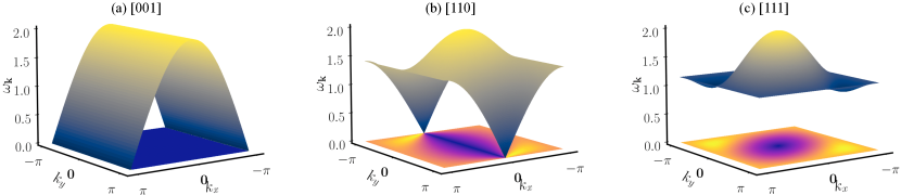
Supplementary Fig. S10: Magnon bands of $H^{(2)}_{s}$ in Eq. (S23) with $\varGamma=0$ for spin polarization in the (a) [001], (b) [110], and (c) [111] directions. Here we set the doping level $\delta=0$ and thereby $P_{\gamma}=0$.

$H^{(2)}_{s}$ is the quadratic term in the Hamiltonian. In the basis of $\mathbb{B}^{\dagger}_{{\bf k}}\equiv(a^{\dagger}_{{\bf k},0},a^{\dagger}_{{\bf k},1},a_{-{\bf k},0},a_{-{\bf k},1})$, it reads

$$\begin{split}H^{(2)}_{s}=&\sum_{{\bf k}}\mathbb{B}^{\dagger}_{{\bf k}}\left(\begin{array}[]{cc}\mathbb{T}_{{\bf k}}&\mathbb{D}_{{\bf k}}\\ \mathbb{D}^{\dagger}_{{\bf k}}&\mathbb{T}^{T}_{-{\bf k}}\end{array}\right)\mathbb{B}_{{\bf k}}+\mathrm{N}_{c}\Re[P_{x}+P_{y}+P_{z}]t-\frac{N\mathrm{N}_{c}D{}}{2}[K+\varGamma{}f(\phi,\theta)],\end{split}$$ (S23)

where $\mathbb{T}_{{\bf k}}$ and $\mathbb{D}_{{\bf k}}$ are $2\times{}2$ matrices:

$$\mathbb{T}_{{\bf k}}=\frac{\kappa D}{4}\left(\begin{array}[]{r|r}&\frac{-K}{2}\left(\cos^{2}\theta\cos^{2}\phi+\sin^{2}\theta\right)+\frac{\varGamma}{2}\sin\theta\sin 2\phi+\\ K+\varGamma{}f(\theta,\phi)&\left[\frac{-K}{2}\left(\sin^{2}\theta\cos^{2}\phi+\cos^{2}\theta\right)+\frac{\varGamma}{2}\cos\theta\sin 2\phi\right]e^{ik_{x}}+\\ &\left[\frac{K}{2}\sin^{2}\phi+\frac{\varGamma}{2}\sin 2\theta\sin^{2}\phi\right]e^{ik_{y}}}{}{}{}{\\ \hline\cr&\\ h.c.}{&K+\varGamma{}f(\theta,\phi)\\ &\end{array}\right)-\frac{t}{2}\left(\begin{array}[]{r|r}\Re[P_{x}]+&-P_{x}^{*}+\\ \Re[P_{y}]+&-P_{y}^{*}e^{-ik_{x}}+\\ \Re[P_{z}]}{}{}{}{&-P_{z}^{*}e^{-ik_{y}}}{}{}{}{\\ \hline\cr&\Re[P_{x}]+\\ h.c.}{&\Re[P_{y}]+\\ &\Re[P_{z}]}{}{}{}{\end{array}\right),$$ (S36)

and

$$\mathbb{D}_{{\bf k}}=\frac{\kappa D}{4}\left(\begin{array}[]{r|r}&\frac{-K}{2}\left(\cos^{2}\theta\cos^{2}\phi-\sin^{2}\theta-i\sin 2\theta\cos\phi\right)+\\ &\frac{-K}{2}\left(\sin^{2}\theta\cos^{2}\phi-\cos^{2}\theta+2i\sin 2\theta\cos\phi\right)e^{ik_{x}}+\\ &-\frac{K}{2}\sin^{2}\phi{}e^{ik_{y}}+\\ &\frac{\varGamma}{2}\left(\sin\theta\sin 2\phi+2i\cos\theta\sin\phi\right)+\\ &\frac{\varGamma}{2}\left(\cos\theta\sin 2\phi-2i\sin\theta\sin\phi\right)e^{ik_{x}}+\\ &-\frac{\varGamma}{2}\left[\sin 2\theta(\cos^{2}\phi+1)+2i\cos 2\theta\cos\phi\right]e^{ik_{y}}}{}{}{}{\\ \hline\cr\frac{-K}{2}\left(\cos^{2}\theta\cos^{2}\phi-\sin^{2}\theta-i\sin 2\theta\cos\phi\right)+&\\ \frac{-K}{2}\left(\sin^{2}\theta\cos^{2}\phi-\cos^{2}\theta+2i\sin 2\theta\cos\phi\right)e^{-ik_{x}}+&\\ -\frac{K}{2}\sin^{2}\phi{}e^{-ik_{y}}+&\\ \frac{\varGamma}{2}\left(\sin\theta\sin 2\phi+2i\cos\theta\sin\phi\right)+&\\ \frac{\varGamma}{2}\left(\cos\theta\sin 2\phi-2i\sin\theta\sin\phi\right)e^{-ik_{x}}+&\\ -\frac{\varGamma}{2}\left[\sin 2\theta(\cos^{2}\phi+1)+2i\cos 2\theta\cos\phi\right]e^{-ik_{y}}}{}{}{}{&\end{array}\right).$$ (S37)

We emphasize that when $\varGamma>0$, the spin polarization direction must be fixed as $\phi=\arccos(\pm{}1/\sqrt{3})$ and $\theta=\pm\pi/4$. It is worth noting that due to the lattice and time-reversal symmetries, in practice, we have $P_{x}=\Re[P_{x}]=P_{y}=P_{z}$. Therefore, we verify from the form of $\mathbb{T}_{{\bf k}}$ that the hole kinetic terms can play a role similar to the ferromagnetic Heisenberg interactions in the spin-wave theory with $J\equiv-\langle{}P_{x}\rangle{}t/\kappa.$

Order-by-disorder

Note that the constant term in Eq. (S23) arises from the zero-point energy contribution of the bosons, i.e., appears because we express this quadratic Hamiltonian in a bosonic BdG form. Therefore, the ground state energy of $\mathcal{H}_{s}$ up to the second order corrections reads

$$\begin{split}E_{s}=&\sum_{{\bf k}}\sum_{n=1,2}\omega_{{\bf k},n}+(2N+1)\mathrm{N}_{c}\Re[P_{x}+P_{y}+P_{z}]t-\frac{N(N+2)\mathrm{N}_{c}}{4}[K+\varGamma{}f_{0}(\phi,\theta)],\end{split}$$ (S38)

where $\omega_{{\bf k},n}^{\prime}s$ is the magnon dispersion. Note that $\omega_{{\bf k},n}$ still depends on $\theta$ and $\phi$ even when $\varGamma=0$, indicating that the $O(3)$ degeneracy at the Kitaev point is lifted by quantum fluctuations. We find that a [001] (or equivalently [100] and [010]) magnetization is more energetically favorable than other directions, see Fig. S9, indicating the presence of a quantum order-by-disorder mechanism.

Supplementary Fig. S11: (a) In a [100] ordered ground state, where the effect of $z$-type (red dashed line) and $y$-type (green dashed line) bonds vanishes effectively, a zero-energy excitation can be constructed by flipping two spins (highlighted by the red shadow) connected by one $x$-type bonds (blue solid lines) into the [$\bar{1}00$] ($\bar{1}=-1$) direction. (b) Arbitrary numbers of zero-energy excitations can be created, leading to a flat magnon band for the [100] polarization. (c) In a [$xy$0] ordered ground state, the effect of $z$-type bonds (red dashed line) vanishes effectively and the honeycomb lattice is reduced into several independent chains formed by $x$- and $y$-type bonds (blue and green solid lines). The mechanism described in (a) and (b) no longer applies to this case. Instead, a zero-energy excitation can be created by rotating all the spins on a single chain (highlighted by the yellow shading) by an arbitrary angle around the $z$-axis. (d) All the spins on each decoupled chain can be rotated freely around the $z$-axis without costing energies, leading to numerous zero-energy excitations and thereby a flat magnon bond for a [$xy$0] polarization. Note that the mechanism described by (c) and (d) is also applicable to the [100] ordered state.

Supplementary Fig. S12: Magnon bands of $H^{(2)}_{s}$ in Eq. (S23) for spin polarization in the [111] direction. (a) $\varGamma=0.05$ and doping level $\delta=0$. (b) $\varGamma=0.05$, $t=10$, and $\delta=0.01$, leading to a self-consistent solution of $P_{x,y,z}=-9.33\times{}10^{-3}$ and $F^{x,y,z}=0.86$.

Flat magnon band in $H^{(2)}_{s}$

When we diagonalize $H^{(2)}_{s}$, we find that the lower magnon band, $\omega_{{\bf k},0}$, is a nearly flat band with almost zero energy, see Figs. S10, regardless of the spin polarization directions. This flat band arises because the semiclassical ground state of the ferromagnetic Kitaev honeycomb model is not necessarily a ferromagnetic order but instead a classical spin liquid. In order words, one can construct numerous zero-energy excitations on top of a ferromagnetically ordered ground state in the semiclassical Kitaev honeycomb model, as demonstrated in Fig. S11. Though we use the [100] and [$xy$0] order as examples to illustrate the zero-energy excitations, the same mechanism is applicable for arbitrary [$xyz$] order. Indeed, one can construct the same type of excitations on top of a [$xyz$] order by fixing the $z$ components of all spins uniform and unchanged. Therefore, one can always observe flat magnon bands for arbitrary $[xyz]$ ordered ground state in the pure Kitaev honeycomb model.

The flat band we discussed above can gain dispersion in two scenarios: (i) a finite positive $\varGamma$ which also forces the polarization direction to be [111], and (ii) a large $t$ with a finite doping level $\delta$ (i.e., a nonzero $P_{\gamma}$). Note that the lower band of $H^{(2)}_{s}$ exhibits gapless Goldstone-like modes even when $\varGamma>0$, as shown in Fig. S12(a), although the system does not have any continuous symmetries to be spontaneously broken. This phenomenon has also been reported in Refs. [59, 40]. The zero-energy modes disappear in the presence of finite doping $\delta$, as shown in Fig. S12(b).

V.0.3 Fourth-order correction to the magnon bands

The appearance of a flat band with zero energy and Goldstone-like modes indicates that $H^{(2)}_{s}$ is insufficient to capture the quantum fluctuations in the system. To properly account for these strong fluctuations, one must consider higher-order corrections from the Holstein-Primakoff expansion, specifically the quartic terms in the spin-wave Hamiltonian $H^{(4)}_{s}$ as (a positive $\varGamma>0$ will force the spin polarization to be fixed as $\phi=\arccos(\pm{}1/\sqrt{3})$ and $\theta=\pm\pi/4$)

$$H^{(4)}_{s}=\sum_{{\bf r}} K\left[4\cos^{2}\theta\sin^{2}\phi{}a^{\dagger}_{{\bf r},0}a_{{\bf r},0}a^{\dagger}_{{\bf r},1}a_{{\bf r},1}+4\sin^{2}\theta\sin^{2}\phi{}a^{\dagger}_{{\bf r}+x,0}a_{{\bf r}+x,0}a^{\dagger}_{{\bf r},1}a_{{\bf r},1}+4\cos^{2}\phi{}a^{\dagger}_{{\bf r}+y,0}a_{{\bf r}+y,0}a^{\dagger}_{{\bf r},1}a_{{\bf r},1}\right]+$$

$$-\varGamma\left[4\sin\theta\sin 2\phi{}a^{\dagger}_{{\bf r},0}a_{{\bf r},0}a^{\dagger}_{{\bf r},1}a_{{\bf r},1}+4\cos\theta\sin 2\phi{}a^{\dagger}_{{\bf r}+x,0}a_{{\bf r}+x,0}a^{\dagger}_{{\bf r},1}a_{{\bf r},1}+4\sin 2\theta\sin^{2}\phi{}a^{\dagger}_{{\bf r}+y,0}a_{{\bf r}+y,0}a^{\dagger}_{{\bf r},1}a_{{\bf r},1}\right]+$$

$$\left\{\left[\frac{K}{2}\left(\cos^{2}\theta\cos^{2}\phi+\sin^{2}\theta\right)-\frac{\varGamma}{2}\sin\theta\sin 2\phi\right]\left(a^{\dagger}_{{\bf r},0}a_{{\bf r},0}a^{\dagger}_{{\bf r},0}a_{{\bf r},1}+a^{\dagger}_{{\bf r},1}a_{{\bf r},1}a^{\dagger}_{{\bf r},1}a_{{\bf r},0}\right)+h.c.\right\}+$$

$$\left\{\left[\frac{K}{2}\left(\cos^{2}\theta\cos^{2}\phi-\sin^{2}\theta-i\sin 2\theta\cos\phi\right)-\frac{\varGamma}{2}\left(\sin\theta\sin 2\phi+2i\cos\theta\sin\phi\right)\right]\left(a^{\dagger}_{{\bf r},0}a_{{\bf r},0}a^{\dagger}_{{\bf r},0}a^{\dagger}_{{\bf r},1}+a^{\dagger}_{{\bf r},1}a_{{\bf r},1}a^{\dagger}_{{\bf r},1}a^{\dagger}_{{\bf r},0}\right)+h.c.\right\}+$$

$$\left\{\left[\frac{K}{2}\left(\sin^{2}\theta\cos^{2}\phi+\cos^{2}\theta\right)-\frac{\varGamma}{2}\cos\theta\sin 2\phi\right]\left(a^{\dagger}_{{\bf r}+x,0}a_{{\bf r}+x,0}a^{\dagger}_{{\bf r}+x,0}a_{{\bf r},1}+a^{\dagger}_{{\bf r},1}a_{{\bf r},1}a^{\dagger}_{{\bf r},1}a_{{\bf r}+x,0}\right)+h.c.\right\}+$$

$$\left\{\left[\frac{K}{2}\left(\sin^{2}\theta\cos^{2}\phi-\cos^{2}\theta+i\sin 2\theta\cos\phi\right)-\frac{\varGamma}{2}\left(\cos\theta\sin 2\phi-2i\sin\theta\sin\phi\right)\right]\left(a^{\dagger}_{{\bf r}+x,0}a_{{\bf r}+x,0}a^{\dagger}_{{\bf r}+x,0}a^{\dagger}_{{\bf r},1}+a^{\dagger}_{{\bf r},1}a_{{\bf r},1}a^{\dagger}_{{\bf r},1}a^{\dagger}_{{\bf r}+x,0}\right)+h.c.\right\}+$$

$$\left\{\left[\frac{K}{2}\sin^{2}\phi-\frac{\varGamma}{2}\sin 2\theta\sin^{2}\phi\right]\left(a^{\dagger}_{{\bf r}+y,0}a_{{\bf r}+y,0}a^{\dagger}_{{\bf r}+y,0}a_{{\bf r},1}+a^{\dagger}_{{\bf r},1}a_{{\bf r},1}a^{\dagger}_{{\bf r},1}a_{{\bf r}+y,0}\right)+h.c.\right\}+$$

$$\left\{\left[\frac{K}{2}\sin^{2}\phi+\frac{\varGamma}{2}\left(\sin 2\theta(\cos^{2}\phi+1)+2i\cos 2\theta\cos\phi\right)\right]\left(a^{\dagger}_{{\bf r}+y,0}a_{{\bf r}+y,0}a^{\dagger}_{{\bf r}+y,0}a^{\dagger}_{{\bf r},1}+a^{\dagger}_{{\bf r},1}a_{{\bf r},1}a^{\dagger}_{{\bf r},1}a^{\dagger}_{{\bf r}+y,0}\right)+h.c.\right\},$$

Note that in this context, we have neglected the fourth-order contributions from the kinetic terms since $P_{\gamma}\sim\delta$ is relatively small in the small doping limit.

By introducing several Hartree-Fock parameters:

$$\begin{array}[]{lll}n_{l}=\frac{1}{\mathrm{N}_{c}}\sum_{\bf k}\langle{}a^{\dagger}_{{\bf k},l}a_{{\bf k},l}\rangle,&\delta_{l}=\frac{1}{\mathrm{N}_{c}}\sum_{\bf k}\langle{}b_{{\bf k},l}a_{{\bf k},l}\rangle,&\\ m_{x}=\frac{1}{\mathrm{N}_{c}}\sum_{\bf k}\langle{}a^{\dagger}_{{\bf k},0}a_{{\bf k},1}\rangle,&m_{y}=\frac{1}{\mathrm{N}_{c}}\sum_{\bf k}e^{ik_{x}}\langle{}a^{\dagger}_{{\bf k},0}a_{{\bf k},1}\rangle,&m_{z}=\frac{1}{\mathrm{N}_{c}}\sum_{\bf k}e^{ik_{y}}\langle{}a^{\dagger}_{{\bf k},0}a_{{\bf k},1}\rangle,\\ \Delta_{x}=\frac{1}{\mathrm{N}_{c}}\sum_{\bf k}\langle{}a_{{\bf k},0}a_{-{\bf k},1}\rangle,&\Delta_{y}=\frac{1}{\mathrm{N}_{c}}\sum_{\bf k}e^{-ik_{x}}\langle{}a_{{\bf k},0}a_{-{\bf k},1}\rangle,&\Delta_{z}=\frac{1}{\mathrm{N}_{c}}\sum_{\bf k}e^{-ik_{y}}\langle{}a_{{\bf k},0}a_{-{\bf k},1}\rangle,\\ \end{array}$$

the terms in $H^{(4)}_{s}$ on a $\alpha$-type bond $\langle({\bf r},0)$, $({\bf r}^{\prime},1)\rangle$ are decomposed (${\bf r}$ is the unit-cell index) as

$$\begin{split}a^{\dagger}_{{\bf r},0}a_{{\bf r},0}a^{\dagger}_{{\bf r}^{\prime},1}a_{{\bf r}^{\prime},1}\rightarrow{}&n_{0}a^{\dagger}_{{\bf r}^{\prime},1}a_{{\bf r}^{\prime},1}+n_{1}a^{\dagger}_{{\bf r},0}a_{{\bf r},0}+n_{1}n_{1}+\Delta_{\alpha}{}a^{\dagger}_{{\bf r},0}a^{\dagger}_{{\bf r}^{\prime},1}+\Delta_{\alpha}^{*}a_{{\bf r},0}a_{{\bf r}^{\prime},1}+|\Delta_{\alpha}|^{2}+m_{\alpha}{}a^{\dagger}_{{\bf r}^{\prime},1}a_{{\bf r},0}+m_{\alpha}^{*}a^{\dagger}_{{\bf r},0}a_{{\bf r}^{\prime},1}+|m_{\alpha}|^{2},\\ a^{\dagger}_{{\bf r},0}a_{{\bf r},0}a^{\dagger}_{{\bf r},0}a_{{\bf r}^{\prime},1}\rightarrow{}&2n_{0}a^{\dagger}_{{\bf r},0}a_{{\bf r}^{\prime},1}+m_{\alpha}a^{\dagger}_{{\bf r},0}a_{{\bf r},0}+m_{\alpha}a_{{\bf r},0}a^{\dagger}_{{\bf r},0}+2n_{0}m_{\alpha}+\delta_{0}^{*}a_{{\bf r},0}a_{{\bf r}^{\prime},1}+\Delta_{\alpha}a^{\dagger}_{{\bf r},0}a^{\dagger}_{{\bf r},0}+\delta_{0}^{*}\Delta_{\alpha},\\ a^{\dagger}_{{\bf r}^{\prime},1}a_{{\bf r}^{\prime},1}a^{\dagger}_{{\bf r}^{\prime},1}a_{{\bf r},0}\rightarrow{}&2n_{1}a^{\dagger}_{{\bf r}^{\prime},1}a_{{\bf r},0}+m_{\alpha}^{*}a^{\dagger}_{{\bf r}^{\prime},1}a_{{\bf r}^{\prime},1}+m_{\alpha}^{*}a_{{\bf r}^{\prime},1}a^{\dagger}_{{\bf r}^{\prime},1}+2n_{1}m_{\alpha}^{*}+\delta_{1}^{*}a_{{\bf r}^{\prime},1}a_{{\bf r},0}+\Delta_{\alpha}a^{\dagger}_{{\bf r}^{\prime},1}a^{\dagger}_{{\bf r}^{\prime},1}+\delta_{1}^{*}\Delta_{\alpha},\\ a^{\dagger}_{{\bf r},0}a_{{\bf r},0}a^{\dagger}_{{\bf r},0}a^{\dagger}_{{\bf r}^{\prime},1}\rightarrow{}&2n_{0}a^{\dagger}_{{\bf r},0}a^{\dagger}_{{\bf r}^{\prime},1}+\Delta_{\alpha}^{*}a^{\dagger}_{{\bf r},0}a_{{\bf r},0}+\Delta_{\alpha}^{*}a_{{\bf r},0}a^{\dagger}_{{\bf r},0}+2n_{0}\Delta_{\alpha}^{*}+\delta_{0}^{*}a^{\dagger}_{{\bf r}^{\prime},1}a_{{\bf r},0}+m_{\alpha}^{*}a^{\dagger}_{{\bf r},0}a^{\dagger}_{{\bf r},0}+\delta_{0}^{*}m_{\alpha}^{*},\\ a^{\dagger}_{{\bf r}^{\prime},1}a_{{\bf r}^{\prime},1}a^{\dagger}_{{\bf r}^{\prime},1}a^{\dagger}_{{\bf r},0}\rightarrow{}&2n_{1}a^{\dagger}_{{\bf r}^{\prime},1}a^{\dagger}_{{\bf r},0}+\Delta_{\alpha}^{*}a^{\dagger}_{{\bf r}^{\prime},1}a_{{\bf r}^{\prime},1}+\Delta_{\alpha}^{*}a_{{\bf r}^{\prime},1}a^{\dagger}_{{\bf r}^{\prime},1}+2n_{1}\Delta_{\alpha}^{*}+\delta_{1}^{*}a^{\dagger}_{{\bf r},0}a_{{\bf r}^{\prime},1}+m_{\alpha}a^{\dagger}_{{\bf r}^{\prime},1}a^{\dagger}_{{\bf r}^{\prime},1}+\delta_{1}^{*}m_{\alpha}.\\ \end{split}$$

Then the quartic interaction terms can be replaced with

$$H^{(4)}_{s}=\delta{}E^{(4)}_{s}+\delta{}H^{(2)}_{s}+...,$$ (S39)

where $\delta{}E^{(4)}_{s}$ and $\delta{}H^{(2)}_{s}$ are the Hartree-Fock corrections to the ground-state energy and magnon spectrum, respectively.

Supplementary Fig. S13: (a,b,c) Magnon bands of $H^{(2)}_{s}+\delta{}H^{(2)}_{s}$ [see corresponding definitions in Eqs. (S23) and (S40)] (a) for spin polarization in the [001] direction with $\varGamma=0$, (b) for that in the [111] direction with $\varGamma=0$, and (c) for that in the [111] direction with $\varGamma=0.05$. Here we set $t=10$ and $\delta=0.01$, leading to self-consistent solutions of (a) $P_{x,y,z}=-9.17\times{}10^{-3}$, $F^{x}=F^{y}=0.79$, and $F^{z}=0.82$, (b) $P_{x,y,z}=-9.17\times{}10^{-3}$ and $F^{x,y,z}=0.83$, and (c) $P_{x,y,z}=-9.33\times{}10^{-3}$ and $F^{x,y,z}=0.86$. (d,e,f) Magnon bands of $H^{(2)}$ only, for comparison. The model parameters and spin polarizations of figures in the same column are the same.

Substituting the above decomposition into the quartic terms in $H^{(4)}_{s}$ leads to

$$\delta{}H^{(2)}_{s}=\sum_{{\bf k}}\mathbb{B}^{\dagger}_{{\bf k}}\left(\begin{array}[]{cc}\delta{}\mathbb{T}_{{\bf k}}&\delta{}\mathbb{D}_{{\bf k}}\\ \delta{}\mathbb{D}^{\dagger}_{{\bf k}}&\delta{}\mathbb{T}^{T}_{-{\bf k}}\end{array}\right)\mathbb{B}_{{\bf k}}.$$ (S40)

Here the explicit form of $\delta\mathbb{T}_{\bf k}$ is

$$\delta\mathbb{T}_{{\bf k}}= D\left(\begin{array}[]{r|r}2n_{1}K+&2m^{*}_{x}\left(K\cos^{2}\theta\sin^{2}\phi-\varGamma\sin\theta\sin 2\phi\right)+\\ -2n_{1}\varGamma(\sin\theta+\cos\theta)\sin 2\phi+&2m^{*}_{y}\left[K\left(\sin^{2}\theta\sin^{2}\phi\right)-\varGamma\cos\theta\sin 2\phi\right]e^{ik_{x}}+\\ -2n_{1}\varGamma\sin 2\theta\sin^{2}\phi}{}{}{}{&2m_{z}^{*}\left[K\cos^{2}\phi-\varGamma\sin 2\theta\sin^{2}\phi\right]e^{ik_{y}}}{}{}{}{\\ \hline\cr&2n_{0}K+\\ h.c.}{&-2n_{0}\varGamma(\sin\theta+\cos\theta)\sin 2\phi+\\ &-2n_{0}\varGamma\sin 2\theta\sin^{2}\phi}{}{}{}{\end{array}\right)+$$ (S47)

$$D\left(\begin{array}[]{r|r}(m_{x}+m_{x}^{*})\left[\frac{K}{2}\left(\cos^{2}\theta\cos^{2}\phi+\sin^{2}\theta\right)-\frac{\varGamma}{2}\sin\theta\sin 2\phi\right]&(n_{0}+n_{1})\left[\frac{K}{2}\left(\cos^{2}\theta\cos^{2}\phi+\sin^{2}\theta\right)-\frac{\varGamma}{2}\sin\theta\sin 2\phi\right]+\\ (m_{y}+m_{y}^{*})\left[\frac{K}{2}\left(\sin^{2}\theta\cos^{2}\phi+\cos^{2}\theta\right)-\frac{\varGamma}{2}\cos\theta\sin 2\phi\right]+&(n_{0}+n_{1})\left[\frac{K}{2}\left(\sin^{2}\theta\cos^{2}\phi+\cos^{2}\theta\right)-\frac{\varGamma}{2}\cos\theta\sin 2\phi\right]e^{ik_{x}}+\\ (m_{z}+m_{z}^{*})\left[\frac{K}{2}\sin^{2}\phi-\frac{\varGamma}{2}\sin 2\theta\sin^{2}\phi\right]}{}{}{}{&(n_{0}+n_{1})\left[\frac{K}{2}\sin^{2}\phi-\frac{\varGamma}{2}\sin 2\theta\sin^{2}\phi\right]e^{ik_{y}}}{}{}{}{\\ \hline\cr&(m_{x}+m_{x}^{*})\left[\frac{K}{2}\left(\cos^{2}\theta\cos^{2}\phi+\sin^{2}\theta\right)-\frac{\varGamma}{2}\sin\theta\sin 2\phi\right]+\\ h.c.}{&(m_{y}+m_{y}^{*})\left[\frac{K}{2}\left(\sin^{2}\theta\cos^{2}\phi+\cos^{2}\theta\right)-\frac{\varGamma}{2}\cos\theta\sin 2\phi\right]+\\ &(m_{z}+m_{z}^{*})\left[\frac{K}{2}\sin^{2}\phi-\frac{\varGamma}{2}\sin 2\theta\sin^{2}\phi\right]}{}{}{}{\end{array}\right)+$$ (S54)

$$D\left(\begin{array}[]{r|r}(\Delta_{x}^{*}+\Delta_{x})\left[\frac{K}{2}\left(\cos^{2}\theta\cos^{2}\phi-\sin^{2}\theta\right)-\frac{\varGamma}{2}\sin\theta\sin 2\phi\right]+&\frac{\delta_{1}^{*}+\delta_{0}}{2}\left[\frac{K}{2}\left(\cos^{2}\theta\cos^{2}\phi-\sin^{2}\theta\right)-\frac{\varGamma}{2}\sin\theta\sin 2\phi\right]+\\ (\Delta_{x}^{*}-\Delta_{x})\left[-i\frac{K}{2}\sin 2\theta\cos\phi-i{\varGamma}\cos\theta\sin\phi\right]+&\frac{\delta_{1}^{*}-\delta_{0}}{2}\left[-i\frac{K}{2}\sin 2\theta\cos\phi-i{\varGamma}\cos\theta\sin\phi\right]+\\ (\Delta_{y}^{*}+\Delta_{y})\left[\frac{K}{2}\left(\sin^{2}\theta\cos^{2}\phi-\cos^{2}\theta\right)-\frac{\varGamma}{2}\cos\theta\sin 2\phi\right]+&\frac{\delta_{1}^{*}+\delta_{0}}{2}\left[\frac{K}{2}\left(\sin^{2}\theta\cos^{2}\phi-\cos^{2}\theta\right)-\frac{\varGamma}{2}\cos\theta\sin 2\phi\right]e^{ik_{x}}+\\ (\Delta_{y}^{*}-\Delta_{y})\left[i\frac{K}{2}\sin 2\theta\cos\phi+i\varGamma\sin\theta\sin\phi\right]+&\frac{\delta_{1}^{*}-\delta_{0}}{2}\left[i\frac{K}{2}\sin 2\theta\cos\phi+i\varGamma\sin\theta\sin\phi\right]e^{ik_{x}}+\\ (\Delta_{z}+\Delta_{z}^{*})\left[\frac{K}{2}\sin^{2}\phi+\frac{\varGamma}{2}\sin 2\theta(\cos^{2}\phi+1)\right]+&\frac{\delta_{0}+\delta_{1}^{*}}{2}\frac{K}{2}\sin^{2}\phi{}e^{ik_{y}}+\\ i(\Delta_{z}^{*}-\Delta_{z})\varGamma\cos 2\theta\cos\phi}{}{}{}{&i\frac{\delta_{1}^{*}-\delta_{0}}{2}\varGamma\cos 2\theta\cos\phi{}e^{ik_{y}}}{}{}{}{\\ \hline\cr&(\Delta_{x}^{*}+\Delta_{x})\left[\frac{K}{2}\left(\cos^{2}\theta\cos^{2}\phi-\sin^{2}\theta\right)-\frac{\varGamma}{2}\sin\theta\sin 2\phi\right]+\\ &(\Delta_{x}^{*}-\Delta_{x})\left[-i\frac{K}{2}\sin 2\theta\cos\phi-i{\varGamma}\cos\theta\sin\phi\right]+\\ h.c.}{&(\Delta_{y}^{*}+\Delta_{y})\left[\frac{K}{2}\left(\sin^{2}\theta\cos^{2}\phi-\cos^{2}\theta\right)-\frac{\varGamma}{2}\cos\theta\sin 2\phi\right]+\\ &(\Delta_{y}^{*}-\Delta_{y})\left[i\frac{K}{2}\sin 2\theta\cos\phi+i\varGamma\sin\theta\sin\phi\right]+\\ &(\Delta_{z}+\Delta_{z}^{*})\left[\frac{K}{2}\sin^{2}\phi+\frac{\varGamma}{2}\sin 2\theta(\cos^{2}\phi+1)\right]+\\ &i(\Delta_{z}^{*}-\Delta_{z})\varGamma\cos 2\theta\cos\phi}{}{}{}{\end{array}\right).$$ (S67)

Similarly,

$$\delta\mathbb{D}_{{\bf k}}= D\left(\begin{array}[]{r|r}&2\Delta_{x}\left[K\cos^{2}\theta\sin^{2}\phi-\varGamma\sin\theta\sin 2\phi\right]+\\ &2\Delta_{y}\left[K\sin^{2}\theta\sin^{2}\phi-\varGamma\cos\theta\sin 2\phi\right]e^{ik_{x}}+\\ &2\Delta_{z}\left[K\cos^{2}\phi{}-\varGamma\sin 2\theta\sin^{2}\phi\right]e^{ik_{y}}+\\ \hline\cr 2\Delta_{x}\left[K\cos^{2}\theta\sin^{2}\phi-\varGamma\sin\theta\sin 2\phi\right]+&\\ 2\Delta_{y}\left[K\sin^{2}\theta\sin^{2}\phi-\varGamma\cos\theta\sin 2\phi\right]e^{-ik_{x}}+&\\ 2\Delta_{z}\left[K\cos^{2}\phi{}-\varGamma\sin 2\theta\sin^{2}\phi\right]e^{-ik_{y}}+&\\ \end{array}\right)+$$ (S74)

$$D\left(\begin{array}[]{r|r}(\Delta_{x}+\Delta_{x}^{*})\left[\frac{K}{2}\left(\cos^{2}\theta\cos^{2}\phi+\sin^{2}\theta\right)-\frac{\varGamma}{2}\sin\theta\sin 2\phi\right]&\frac{\delta_{0}+\delta_{1}}{2}\left[\frac{K}{2}\left(\cos^{2}\theta\cos^{2}\phi+\sin^{2}\theta\right)-\frac{\varGamma}{2}\sin\theta\sin 2\phi\right]+\\ (\Delta_{y}+\Delta_{y}^{*})\left[\frac{K}{2}\left(\sin^{2}\theta\cos^{2}\phi+\cos^{2}\theta\right)-\frac{\varGamma}{2}\cos\theta\sin 2\phi\right]+&\frac{\delta_{0}+\delta_{1}}{2}\left[\frac{K}{2}\left(\sin^{2}\theta\cos^{2}\phi+\cos^{2}\theta\right)-\frac{\varGamma}{2}\cos\theta\sin 2\phi\right]e^{ik_{x}}+\\ (\Delta_{z}+\Delta_{z}^{*})\left[\frac{K}{2}\sin^{2}\phi-\frac{\varGamma}{2}\sin 2\theta\sin^{2}\phi\right]}{}{}{}{&\frac{\delta_{0}+\delta_{1}}{2}\left[\frac{K}{2}\sin^{2}\phi-\frac{\varGamma}{2}\sin 2\theta\sin^{2}\phi\right]e^{ik_{y}}}{}{}{}{\\ \hline\cr\frac{\delta_{0}+\delta_{1}}{2}\left[\frac{K}{2}\left(\cos^{2}\theta\cos^{2}\phi+\sin^{2}\theta\right)-\frac{\varGamma}{2}\sin\theta\sin 2\phi\right]+&(\Delta_{x}+\Delta_{x}^{*})\left[\frac{K}{2}\left(\cos^{2}\theta\cos^{2}\phi+\sin^{2}\theta\right)-\frac{\varGamma}{2}\sin\theta\sin 2\phi\right]\\ \frac{\delta_{0}+\delta_{1}}{2}\left[\frac{K}{2}\left(\sin^{2}\theta\cos^{2}\phi+\cos^{2}\theta\right)-\frac{\varGamma}{2}\cos\theta\sin 2\phi\right]e^{-ik_{x}}+&(\Delta_{y}+\Delta_{y}^{*})\left[\frac{K}{2}\left(\sin^{2}\theta\cos^{2}\phi+\cos^{2}\theta\right)-\frac{\varGamma}{2}\cos\theta\sin 2\phi\right]+\\ \frac{\delta_{0}+\delta_{1}}{2}\left[\frac{K}{2}\sin^{2}\phi-\frac{\varGamma}{2}\sin 2\theta\sin^{2}\phi\right]e^{-ik_{y}}}{}{}{}{&(\Delta_{z}+\Delta_{z}^{*})\left[\frac{K}{2}\sin^{2}\phi-\frac{\varGamma}{2}\sin 2\theta\sin^{2}\phi\right]}{}{}{}{\\ \end{array}\right)+$$ (S81)

$$D\left(\begin{array}[]{r|r}m^{*}_{x}\frac{K}{2}\left(\cos^{2}\theta\cos^{2}\phi-\sin^{2}\theta-i\sin 2\theta\cos\phi\right)+&(n_{0}+n_{1})\frac{K}{2}\left(\cos^{2}\theta\cos^{2}\phi-\sin^{2}\theta-i\sin 2\theta\cos\phi\right)+\\ -m^{*}_{x}\frac{\varGamma}{2}\left(\sin\theta\sin 2\phi+2i\cos\theta\sin\phi\right)+&-(n_{0}+n_{1})\frac{\varGamma}{2}\left(\sin\theta\sin 2\phi+2i\cos\theta\sin\phi\right)+\\ m^{*}_{y}\frac{K}{2}\left(\sin^{2}\theta\cos^{2}\phi-\cos^{2}\theta+i\sin 2\theta\cos\phi\right)+&(n_{0}+n_{1})\frac{K}{2}\left(\sin^{2}\theta\cos^{2}\phi-\cos^{2}\theta+i\sin 2\theta\cos\phi\right)e^{ik_{x}}+\\ -m^{*}_{y}\frac{\varGamma}{2}\left(\cos\theta\sin 2\phi-2i\sin\theta\sin\phi\right)+&-(n_{0}+n_{1})\frac{\varGamma}{2}\left(\cos\theta\sin 2\phi-2i\sin\theta\sin\phi\right)e^{ik_{x}}+\\ m^{*}_{z}\frac{K}{2}\sin^{2}\phi+&(n_{0}+n_{1})\frac{K}{2}\sin^{2}\phi{}e^{ik_{y}}+\\ m^{*}_{z}\frac{\varGamma}{2}\left(\sin 2\theta(\cos^{2}\phi+1)+2i\cos 2\theta\cos\phi\right)}{}{}{}{&(n_{0}+n_{1})\frac{\varGamma}{2}\left(\sin 2\theta(\cos^{2}\phi+1)+2i\cos 2\theta\cos\phi\right)e^{ik_{y}}}{}{}{}{\\ \hline\cr(n_{0}+n_{1})\frac{K}{2}\left(\cos^{2}\theta\cos^{2}\phi-\sin^{2}\theta-i\sin 2\theta\cos\phi\right)+&m_{x}\frac{K}{2}\left(\cos^{2}\theta\cos^{2}\phi-\sin^{2}\theta-i\sin 2\theta\cos\phi\right)+\\ -(n_{0}+n_{1})\frac{\varGamma}{2}\left(\sin\theta\sin 2\phi+2i\cos\theta\sin\phi\right)+&-m_{x}\frac{\varGamma}{2}\left(\sin\theta\sin 2\phi+2i\cos\theta\sin\phi\right)+\\ (n_{0}+n_{1})\frac{K}{2}\left(\sin^{2}\theta\cos^{2}\phi-\cos^{2}\theta+i\sin 2\theta\cos\phi\right)e^{-ik_{x}}+&m_{y}\frac{K}{2}\left(\sin^{2}\theta\cos^{2}\phi-\cos^{2}\theta+i\sin 2\theta\cos\phi\right)+\\ -(n_{0}+n_{1})\frac{\varGamma}{2}\left(\cos\theta\sin 2\phi-2i\sin\theta\sin\phi\right)e^{-ik_{x}}+&-m_{y}\frac{\varGamma}{2}\left(\cos\theta\sin 2\phi-2i\sin\theta\sin\phi\right)+\\ (n_{0}+n_{1})\frac{K}{2}\sin^{2}\phi{}e^{-ik_{y}}+&m_{z}\frac{K}{2}\sin^{2}\phi+\\ (n_{0}+n_{1})\frac{\varGamma}{2}\left(\sin 2\theta(\cos^{2}\phi+1)+2i\cos 2\theta\cos\phi\right)e^{-ik_{y}}}{}{}{}{&m_{z}\frac{\varGamma}{2}\left(\sin 2\theta(\cos^{2}\phi+1)+2i\cos 2\theta\cos\phi\right)}{}{}{}{\end{array}\right).$$ (S94)

And the fourth-order correction to the ground-state energy is

$$\delta{}E^{(4)}_{s}=\sum_{\mathbf{k}} 4\left[K-\varGamma(\sin\theta\sin 2\phi+\cos\theta\sin 2\phi+4\sin 2\theta\sin^{2}\phi)\right]4n_{0}n_{1}+4\left(K\cos^{2}\theta\sin^{2}\phi{}-\varGamma\sin\theta\sin 2\phi\right)\left(|m_{x}|^{2}+|\Delta_{x}|^{2}\right)+$$

$$4\left(K\sin^{2}\theta\sin^{2}\phi{}-\varGamma\cos\theta\sin 2\phi\right)\left(|m_{y}|^{2}+|\Delta_{y}|^{2}\right)+4\left(K\cos^{2}\phi{}-\varGamma\sin 2\theta\sin^{2}\phi\right)\left(|m_{z}|^{2}+|\Delta_{z}|^{2}\right)+$$

$$\left[\frac{K}{2}\left(\cos^{2}\theta\cos^{2}\phi+\sin^{2}\theta\right)-\frac{\varGamma}{2}\sin\theta\sin 2\phi\right]\left(2n_{0}m_{x}+2n_{1}m_{x}^{*}+\delta_{0}^{*}\Delta_{x}+\delta_{1}^{*}\Delta_{x}+c.c.\right)+$$

$$\left[\frac{K}{2}\left(\cos^{2}\theta\cos^{2}\phi+\sin^{2}\theta\right)-\frac{\varGamma}{2}\sin\theta\sin 2\phi\right]\left(2n_{0}m_{x}+2n_{1}m_{x}^{*}+\delta_{0}^{*}\Delta_{x}+\delta_{1}^{*}\Delta_{x}+c.c.\right)+$$

$$\left[\frac{K}{2}\sin^{2}\phi-\frac{\varGamma}{2}\sin 2\theta\sin^{2}\phi\right]\left(2n_{0}m_{z}+2n_{1}m_{z}^{*}+\delta_{0}^{*}\Delta_{z}+\delta_{1}^{*}\Delta_{z}+c.c.\right)+$$

$$\left[\frac{K}{2}\sin^{2}\phi-\frac{\varGamma}{2}\sin 2\theta\sin^{2}\phi\right]\left(2n_{0}m_{z}+2n_{1}m_{z}^{*}+\delta_{0}^{*}\Delta_{z}+\delta_{1}^{*}\Delta_{z}+c.c.\right)+$$

$$\left\{\left[\frac{K}{2}\left(\cos^{2}\theta\cos^{2}\phi-\sin^{2}\theta-i\sin 2\theta\cos\phi\right)-\frac{\varGamma}{2}\left(\sin\theta\sin 2\phi+2i\cos\theta\sin\phi\right)\right]\left(2n_{0}\Delta_{x}^{*}+2n_{1}\Delta_{x}^{*}+\delta_{0}^{*}m_{x}^{*}+\delta_{1}^{*}m_{x}\right)+c.c.\right\}+$$

$$\left\{\left[\frac{K}{2}\left(\sin^{2}\theta\cos^{2}\phi-\cos^{2}\theta+i\sin 2\theta\cos\phi\right)-\frac{\varGamma}{2}\left(\cos\theta\sin 2\phi-2i\sin\theta\sin\phi\right)\right]\left(2n_{0}\Delta_{y}^{*}+2n_{1}\Delta_{y}^{*}+\delta_{0}^{*}m_{y}^{*}+\delta_{1}^{*}m_{y}\right)+c.c.\right\}+$$

$$\left\{\left[\frac{K}{2}\sin^{2}\phi+\frac{\varGamma}{2}\left(\sin 2\theta(\cos^{2}\phi+1)+2i\cos 2\theta\cos\phi\right)\right]\left(2n_{0}\Delta_{z}^{*}+2n_{1}\Delta_{z}^{*}+\delta_{0}^{*}m_{z}^{*}+\delta_{1}^{*}m_{z}\right)+c.c.\right\}$$

In the end, we would like to comment that the inclusion of $\delta H^{(2)}_{s}$ leads to several important effects in the spin-wave theory. In Fig S13, we show the magnon bands corrected by the fourth-order term $\delta H^{(2)}_{s}$. We find that $\delta H^{(2)}_{s}$ significantly changes the dispersions of both the lower and upper magnon bands. In particular, the lower band gains much more dispersion, as shown in Fig. S13(a) and (b). Furthermore, the energy gap between the lower and upper magnon bands becomes closed due to the fourth-order corrections when $\varGamma$ vanishes, see Fig. S13(b). It indicates that the topological properties of the magnon bands are also changed by $\delta{}H^{(2)}_{s}$. Finally, a finite $\varGamma$ can reopen the energy gap, as shown in Fig. S13(c).

Supplementary Fig. S14: Zigzag order induced by mobile holes. Real-space magnetization $\langle{}S^{z}_{j}\rangle$ ($\langle{}S^{x}_{j}\rangle$ and $\langle{}S^{y}_{j}\rangle$ are similar) profiles for (a, b) $t$-$K$-$\varGamma$ model on YC3 cylinders and (c,d) $t$-$K$-$J_{3}$ model ($\varGamma=0$) on YC4 cylinders. Here $J_{3}$ is the 3rd NN antiferromagnetic Heisenberg exchange, $K=1$, and the doping level is $\delta\approx 0.015$. Positive and negative magnetic moments are shown by red and blue dots, respectively, whose radius scales with the magnitude of magnetization $|\langle{}S^{z}_{j}\rangle|$, such that $|\langle{}S^{z}_{j}\rangle|\approx 0.06$ in the two middle columns in (b).

Supplementary Note 4: Zigzag order

Motivated by the experimental Kitaev materials, we discuss the effect of hole doping on the zigzag ordered state. Previous studies [29, 45, 47] report that the $K$-$\varGamma$ model alone is insufficient to support a zigzag order, even with a dominant antiferromagnetic $\varGamma<0$. Our simulations are consistent with these findings, as we observe something like spiral and/or incommensurate orders rather than zigzag order up to $\varGamma=-5K$, see Fig. S14(a). On the other hand, the $t$-$K$-$\varGamma$ model at a doping level $\delta\approx 0.01$ can stabilize the zigzag ordered phase with a moderate $t\approx{}0.2K$ with $\varGamma=-5K$, as shown in Fig. S14(b). This is attributed to that the hole kinetic terms act as a ferromagnetic Heisenberg exchange effectively, $J\sim{}|t|\delta{}$, which can prompt a zigzag order in the $K$-$\varGamma$ model [65].

We find that a relatively large value of $|\varGamma|>K$ is required to achieve a zigzag order in the $t$-$K$-$\varGamma$ model, which might be due to the usage of narrow cylindrical geometries in the DMRG simulations [41]. We anticipate that this value will significantly decrease in the two-dimensional limit. Alternatively, we introduce a small third NN antiferromagnetic Heisenberg exchange $J_{3}<0$ on top of the $t$-$K$ ($\varGamma=0$) model, which has shown to be sufficient to drive the system to a zigzag ordered phase [32, 34, 46], even on narrow cylinders. We find that in this scenario, a small $t$ can also enhance the stability of the zigzag phase. For instance, when $J_{3}=-0.07K$, a doping level of $\delta\approx{}0.01$ and a hopping strength of $t=0.2K$ can approximately double the magnitude of zigzag order compared to the case at $t\rightarrow{}0$. Overall, our results suggest that a zigzag order can be more easily stabilized in the $K$-$\varGamma$ ($K$-$J_{3}$) model by supplementing it with a moderate hole kinetic term $t$ as well as small hole doping. Nevertheless, it is worth noting that if the hopping strength $t$ dominates over the antiferromagnetic interactions of $\varGamma<0$ ($J_{3}<0$), the system still undergoes a ferromagnetic ordering transition.

References

• Auerbach [1998] A. Auerbach, Interacting electrons and quantum magnetism (Springer Science & Business Media, 1998).
• Mattis [2006] D. C. Mattis, The Theory of Magnetism Made Simple: An Introduction to Physical Concepts and to Some Useful Mathematical Methods (World Scientific Publishing Company, 2006).
• Nagaoka [1966] Y. Nagaoka, Ferromagnetism in a narrow, almost half-filled $s$ band, Phys. Rev. 147, 392 (1966).
• Dehollain et al. [2020] J. P. Dehollain, U. Mukhopadhyay, V. P. Michal, Y. Wang, B. Wunsch, C. Reichl, W. Wegscheider, M. S. Rudner, E. Demler, and L. M. Vandersypen, Nagaoka ferromagnetism observed in a quantum dot plaquette, Nature 579, 528 (2020).
• Ciorciaro et al. [2023] L. Ciorciaro, T. Smolenski, I. Morera, N. Kiper, S. Hiestand, M. Kroner, Y. Zhang, K. Watanabe, T. Taniguchi, E. Demler, and A. Imamoglu, Kinetic Magnetism in Triangular Moiré Materials, arXiv:2305.02150  (2023).
• Anderson [1973] P. W. Anderson, Resonating valence bonds: A new kind of insulator?, Mater. Res. Bull. 8, 153 (1973).
• Anderson [1987] P. W. Anderson, The resonating valence bond state in La2CuO4 and superconductivity, Science 235, 1196 (1987).
• Lee [2008] P. A. Lee, An end to the drought of quantum spin liquids, Science 321, 1306 (2008).
• Balents [2010] L. Balents, Spin liquids in frustrated magnets, Nature 464, 199 (2010).
• Savary and Balents [2016] L. Savary and L. Balents, Quantum spin liquids: a review, Rep. Prog. Phys. 80, 016502 (2016).
• Zhou et al. [2017] Y. Zhou, K. Kanoda, and T.-K. Ng, Quantum spin liquid states, Rev. Mod. Phys. 89, 025003 (2017).
• Knolle and Moessner [2019] J. Knolle and R. Moessner, A field guide to spin liquids, Annu. Rev. Condens. Matter Phys. 10, 451 (2019).
• Broholm et al. [2020] C. Broholm, R. J. Cava, S. A. Kivelson, D. G. Nocera, M. R. Norman, and T. Senthil, Quantum spin liquids, Science 367 (2020).
• Kitaev [2006] A. Kitaev, Anyons in an exactly solved model and beyond, Annals of Physics 321, 2 (2006), january Special Issue.
• Choi et al. [2012] S. K. Choi, R. Coldea, A. N. Kolmogorov, T. Lancaster, I. I. Mazin, S. J. Blundell, P. G. Radaelli, Y. Singh, P. Gegenwart, K. R. Choi, S.-W. Cheong, P. J. Baker, C. Stock, and J. Taylor, Spin waves and revised crystal structure of honeycomb iridate ${\mathrm{na}}_{2}{\mathrm{iro}}_{3}$Phys. Rev. Lett. 108, 127204 (2012).
• Cao et al. [2013] G. Cao, T. F. Qi, L. Li, J. Terzic, V. S. Cao, S. J. Yuan, M. Tovar, G. Murthy, and R. K. Kaul, Evolution of magnetism in the single-crystal honeycomb iridates $({\text{na}}_{1-x}$li${}_{x}{)}_{2}\text{Ir}{\text{o}}_{3}$Phys. Rev. B 88, 220414 (2013).
• Manni et al. [2014] S. Manni, S. Choi, I. I. Mazin, R. Coldea, M. Altmeyer, H. O. Jeschke, R. Valentí, and P. Gegenwart, Effect of isoelectronic doping on the honeycomb-lattice iridate ${A}_{2}$ ${\mathrm{iro}}_{3}$Phys. Rev. B 89, 245113 (2014).
• Takagi et al. [2019] H. Takagi, T. Takayama, G. Jackeli, G. Khaliullin, and S. E. Nagler, Concept and realization of kitaev quantum spin liquids, Nature Reviews Physics 1, 264 (2019).
• Plumb et al. [2014] K. W. Plumb, J. P. Clancy, L. J. Sandilands, V. V. Shankar, Y. F. Hu, K. S. Burch, H.-Y. Kee, and Y.-J. Kim, $\alpha-{\mathrm{rucl}}_{3}$: A spin-orbit assisted mott insulator on a honeycomb lattice, Phys. Rev. B 90, 041112 (2014).
• Sears et al. [2015] J. A. Sears, M. Songvilay, K. W. Plumb, J. P. Clancy, Y. Qiu, Y. Zhao, D. Parshall, and Y.-J. Kim, Magnetic order in $\alpha-{\text{rucl}}_{3}$: A honeycomb-lattice quantum magnet with strong spin-orbit coupling, Phys. Rev. B 91, 144420 (2015).
• Sandilands et al. [2015] L. J. Sandilands, Y. Tian, K. W. Plumb, Y.-J. Kim, and K. S. Burch, Scattering continuum and possible fractionalized excitations in $\alpha\text{$-$}{\mathrm{rucl}}_{3}$Phys. Rev. Lett. 114, 147201 (2015).
• Banerjee et al. [2016] A. Banerjee, C. Bridges, J.-Q. Yan, A. Aczel, L. Li, M. Stone, G. Granroth, M. Lumsden, Y. Yiu, J. Knolle, et al., Proximate kitaev quantum spin liquid behaviour in a honeycomb magnet, Nature materials 15, 733 (2016).
• Do et al. [2017] S.-H. Do, S.-Y. Park, J. Yoshitake, J. Nasu, Y. Motome, Y. S. Kwon, D. Adroja, D. Voneshen, K. Kim, T.-H. Jang, et al., Majorana fermions in the kitaev quantum spin system $\alpha$-rucl 3, Nature Physics 13, 1079 (2017).
• Baek et al. [2017] S.-H. Baek, S.-H. Do, K.-Y. Choi, Y. S. Kwon, A. U. B. Wolter, S. Nishimoto, J. van den Brink, and B. Büchner, Evidence for a field-induced quantum spin liquid in $\alpha$-${\mathrm{rucl}}_{3}$Phys. Rev. Lett. 119, 037201 (2017).
• Zheng et al. [2017] J. Zheng, K. Ran, T. Li, J. Wang, P. Wang, B. Liu, Z.-X. Liu, B. Normand, J. Wen, and W. Yu, Gapless spin excitations in the field-induced quantum spin liquid phase of $\alpha\text{$-$}{\mathrm{rucl}}_{3}$Phys. Rev. Lett. 119, 227208 (2017).
• Jackeli and Khaliullin [2009] G. Jackeli and G. Khaliullin, Mott insulators in the strong spin-orbit coupling limit: from Heisenberg to a quantum compass and Kitaev models, Physical Review Letters 102, 017205 (2009).
• Chaloupka et al. [2010] J. c. v. Chaloupka, G. Jackeli, and G. Khaliullin, Kitaev-heisenberg model on a honeycomb lattice: Possible exotic phases in iridium oxides ${A}_{2}{\mathrm{iro}}_{3}$Phys. Rev. Lett. 105, 027204 (2010).
• Katukuri et al. [2014] V. M. Katukuri, S. Nishimoto, V. Yushankhai, A. Stoyanova, H. Kandpal, S. Choi, R. Coldea, I. Rousochatzakis, L. Hozoi, and J. Van Den Brink, Kitaev interactions between j= 1/2 moments in honeycomb na2iro3 are large and ferromagnetic: insights from ab initio quantum chemistry calculations, New Journal of Physics 16, 013056 (2014).
• Rau et al. [2014] J. G. Rau, E. K.-H. Lee, and H.-Y. Kee, Generic spin model for the honeycomb iridates beyond the kitaev limit, Phys. Rev. Lett. 112, 077204 (2014).
• Rau et al. [2016] J. G. Rau, E. K.-H. Lee, and H.-Y. Kee, Spin-orbit physics giving rise to novel phases in correlated systems: Iridates and related materials, Annual Review of Condensed Matter Physics 7, 195 (2016).
• Trebst and Hickey [2022] S. Trebst and C. Hickey, Kitaev materials, Physics Reports 950, 1 (2022).
• Winter et al. [2016] S. M. Winter, Y. Li, H. O. Jeschke, and R. Valentí, Challenges in design of kitaev materials: Magnetic interactions from competing energy scales, Phys. Rev. B 93, 214431 (2016).
• Winter et al. [2017a] S. M. Winter, A. A. Tsirlin, M. Daghofer, J. van den Brink, Y. Singh, P. Gegenwart, and R. Valentí, Models and materials for generalized kitaev magnetism, Journal of Physics: Condensed Matter 29, 493002 (2017a).
• Winter et al. [2017b] S. M. Winter, K. Riedl, P. A. Maksimov, A. L. Chernyshev, A. Honecker, and R. Valentí, Breakdown of magnons in a strongly spin-orbital coupled magnet, Nature communications 8, 1152 (2017b).
• Hermanns et al. [2018] M. Hermanns, I. Kimchi, and J. Knolle, Physics of the kitaev model: Fractionalization, dynamic correlations, and material connections, Annual Review of Condensed Matter Physics 9, 17 (2018).
• Chaloupka et al. [2013] J. c. v. Chaloupka, G. Jackeli, and G. Khaliullin, Zigzag magnetic order in the iridium oxide ${\mathrm{na}}_{2}{\mathrm{iro}}_{3}$Phys. Rev. Lett. 110, 097204 (2013).
• Yamaji et al. [2016] Y. Yamaji, T. Suzuki, T. Yamada, S.-i. Suga, N. Kawashima, and M. Imada, Clues and criteria for designing a kitaev spin liquid revealed by thermal and spin excitations of the honeycomb iridate ${\mathrm{na}}_{2}{\mathrm{iro}}_{3}$Phys. Rev. B 93, 174425 (2016).
• Song et al. [2016] X.-Y. Song, Y.-Z. You, and L. Balents, Low-energy spin dynamics of the honeycomb spin liquid beyond the kitaev limit, Phys. Rev. Lett. 117, 037209 (2016).
• Gohlke et al. [2017] M. Gohlke, R. Verresen, R. Moessner, and F. Pollmann, Dynamics of the kitaev-heisenberg model, Phys. Rev. Lett. 119, 157203 (2017).
• Gohlke et al. [2020] M. Gohlke, L. E. Chern, H.-Y. Kee, and Y. B. Kim, Emergence of nematic paramagnet via quantum order-by-disorder and pseudo-goldstone modes in kitaev magnets, Phys. Rev. Res. 2, 043023 (2020).
• Wang et al. [2019] J. Wang, B. Normand, and Z.-X. Liu, One proximate kitaev spin liquid in the $k\text{$-$}j\text{$-$}\mathrm{\Gamma}$ model on the honeycomb lattice, Phys. Rev. Lett. 123, 197201 (2019).
• Buessen and Kim [2021] F. L. Buessen and Y. B. Kim, Functional renormalization group study of the kitaev-$\mathrm{\Gamma}$ model on the honeycomb lattice and emergent incommensurate magnetic correlations, Phys. Rev. B 103, 184407 (2021).
• Zhang et al. [2021] S.-S. Zhang, G. B. Halász, W. Zhu, and C. D. Batista, Variational study of the kitaev-heisenberg-gamma model, Phys. Rev. B 104, 014411 (2021).
• Li et al. [2022] J.-W. Li, N. Rao, J. von Delft, L. Pollet, and K. Liu, Tangle of spin double helices in the honeycomb kitaev-$\gamma$ model (2022), arXiv:2206.08946 [cond-mat.str-el] .
• Janssen et al. [2017] L. Janssen, E. C. Andrade, and M. Vojta, Magnetization processes of zigzag states on the honeycomb lattice: Identifying spin models for $\alpha\text{$-$}{\mathrm{rucl}}_{3}$ and ${\mathrm{na}}_{2}{\mathrm{iro}}_{3}$Phys. Rev. B 96, 064430 (2017).
• Catuneanu et al. [2018] A. Catuneanu, Y. Yamaji, G. Wachtel, Y. B. Kim, and H.-Y. Kee, Path to stable quantum spin liquids in spin-orbit coupled correlated materials, npj Quantum Materials 3, 23 (2018).
• Gohlke et al. [2018] M. Gohlke, G. Wachtel, Y. Yamaji, F. Pollmann, and Y. B. Kim, Quantum spin liquid signatures in kitaev-like frustrated magnets, Phys. Rev. B 97, 075126 (2018).
• Willans et al. [2011] A. J. Willans, J. T. Chalker, and R. Moessner, Site dilution in the kitaev honeycomb model, Phys. Rev. B 84, 115146 (2011).
• Halász et al. [2014] G. B. Halász, J. T. Chalker, and R. Moessner, Doping a topological quantum spin liquid: Slow holes in the kitaev honeycomb model, Phys. Rev. B 90, 035145 (2014).
• You et al. [2012] Y.-Z. You, I. Kimchi, and A. Vishwanath, Doping a spin-orbit mott insulator: Topological superconductivity from the kitaev-heisenberg model and possible application to (na2/li2)iro3Phys. Rev. B 86, 085145 (2012).
• Hyart et al. [2012] T. Hyart, A. R. Wright, G. Khaliullin, and B. Rosenow, Competition between $d$-wave and topological $p$-wave superconducting phases in the doped kitaev-heisenberg model, Phys. Rev. B 85, 140510 (2012).
• Okamoto [2013] S. Okamoto, Global phase diagram of a doped kitaev-heisenberg model, Phys. Rev. B 87, 064508 (2013).
• Scherer et al. [2014] D. D. Scherer, M. M. Scherer, G. Khaliullin, C. Honerkamp, and B. Rosenow, Unconventional pairing and electronic dimerization instabilities in the doped kitaev-heisenberg model, Phys. Rev. B 90, 045135 (2014).
• Peng et al. [2021] C. Peng, Y.-F. Jiang, T. P. Devereaux, and H.-C. Jiang, Precursor of pair-density wave in doping kitaev spin liquid on the honeycomb lattice, npj Quantum Materials 6, 64 (2021).
• White [1992] S. R. White, Density matrix formulation for quantum renormalization groups, Phys. Rev. Lett. 69, 2863 (1992).
• White [1993] S. R. White, Density-matrix algorithms for quantum renormalization groups, Phys. Rev. B 48, 10345 (1993).
• Shender [1982] E. Shender, Antiferromagnetic garnets with fluctuationally interacting sublattices, Zh. Eksp. Teor. Fiz. 83, 326 (1982).
• Henley [1989] C. L. Henley, Ordering due to disorder in a frustrated vector antiferromagnet, Phys. Rev. Lett. 62, 2056 (1989).
• Joshi [2018] D. G. Joshi, Topological excitations in the ferromagnetic kitaev-heisenberg model, Phys. Rev. B 98, 060405 (2018).
• McClarty et al. [2018] P. A. McClarty, X.-Y. Dong, M. Gohlke, J. G. Rau, F. Pollmann, R. Moessner, and K. Penc, Topological magnons in kitaev magnets at high fields, Phys. Rev. B 98, 060404 (2018).
• Banerjee et al. [2017] A. Banerjee, J. Yan, J. Knolle, C. A. Bridges, M. B. Stone, M. D. Lumsden, D. G. Mandrus, D. A. Tennant, R. Moessner, and S. E. Nagler, Neutron scattering in the proximate quantum spin liquid $\alpha$-rucl3, Science 356, 1055 (2017).
• Wang et al. [2017] W. Wang, Z.-Y. Dong, S.-L. Yu, and J.-X. Li, Theoretical investigation of magnetic dynamics in $\alpha-{\mathrm{rucl}}_{3}$Phys. Rev. B 96, 115103 (2017).
• Ran et al. [2017] K. Ran, J. Wang, W. Wang, Z.-Y. Dong, X. Ren, S. Bao, S. Li, Z. Ma, Y. Gan, Y. Zhang, J. T. Park, G. Deng, S. Danilkin, S.-L. Yu, J.-X. Li, and J. Wen, Spin-wave excitations evidencing the kitaev interaction in single crystalline $\alpha\text{$-$}{\mathrm{rucl}}_{3}$Phys. Rev. Lett. 118, 107203 (2017).
• Shitade et al. [2009] A. Shitade, H. Katsura, J. Kuneš, X.-L. Qi, S.-C. Zhang, and N. Nagaosa, Quantum spin hall effect in a transition metal oxide ${\mathrm{na}}_{2}{\mathrm{iro}}_{3}$Phys. Rev. Lett. 102, 256403 (2009).
• Laubach et al. [2017] M. Laubach, J. Reuther, R. Thomale, and S. Rachel, Three-band hubbard model for ${\mathrm{na}}_{2}{\mathrm{iro}}_{3}$: Topological insulator, zigzag antiferromagnet, and kitaev-heisenberg material, Phys. Rev. B 96, 121110 (2017).
• Putikka et al. [1992] W. O. Putikka, M. U. Luchini, and M. Ogata, Ferromagnetism in the two-dimensional t-j model, Phys. Rev. Lett. 69, 2288 (1992).
• Cookmeyer and Moore [2018] T. Cookmeyer and J. E. Moore, Spin-wave analysis of the low-temperature thermal hall effect in the candidate kitaev spin liquid $\alpha-{RuCl}_{3}$Phys. Rev. B 98, 060412 (2018).
• Jayaprakash et al. [1989] C. Jayaprakash, H. R. Krishnamurthy, and S. Sarker, Mean-field theory for the t-j model, Phys. Rev. B 40, 2610 (1989).
• Arovas and Auerbach [1988] D. P. Arovas and A. Auerbach, Functional integral theories of low-dimensional quantum heisenberg models, Phys. Rev. B 38, 316 (1988).
• Auerbach and Arovas [1988] A. Auerbach and D. P. Arovas, Spin dynamics in the square-lattice antiferromagnet, Phys. Rev. Lett. 61, 617 (1988).
• Sachdev [1992] S. Sachdev, Kagome´- and triangular-lattice heisenberg antiferromagnets: Ordering from quantum fluctuations and quantum-disordered ground states with unconfined bosonic spinons, Phys. Rev. B 45, 12377 (1992).
• Holstein and Primakoff [1940] T. Holstein and H. Primakoff, Field dependence of the intrinsic domain magnetization of a ferromagnet, Phys. Rev. 58, 1098 (1940).
• Samarakoon et al. [2017] A. M. Samarakoon, A. Banerjee, S.-S. Zhang, Y. Kamiya, S. E. Nagler, D. A. Tennant, S.-H. Lee, and C. D. Batista, Comprehensive study of the dynamics of a classical kitaev spin liquid, Phys. Rev. B 96, 134408 (2017).
• Chernyshev and Zhitomirsky [2009] A. L. Chernyshev and M. E. Zhitomirsky, Spin waves in a triangular lattice antiferromagnet: Decays, spectrum renormalization, and singularities, Phys. Rev. B 79, 144416 (2009).
• Thouless et al. [1982] D. J. Thouless, M. Kohmoto, M. P. Nightingale, and M. den Nijs, Quantized hall conductance in a two-dimensional periodic potential, Phys. Rev. Lett. 49, 405 (1982).
• Fukui et al. [2005] T. Fukui, Y. Hatsugai, and H. Suzuki, Chern numbers in discretized brillouin zone: Efficient method of computing (spin) hall conductances, Journal of the Physical Society of Japan 74, 1674 (2005).
• Zaletel et al. [2015] M. P. Zaletel, R. S. K. Mong, C. Karrasch, J. E. Moore, and F. Pollmann, Time-evolving a matrix product state with long-ranged interactions, Phys. Rev. B 91, 165112 (2015).
• Zhu et al. [2018] Z. Zhu, I. Kimchi, D. N. Sheng, and L. Fu, Robust non-abelian spin liquid and a possible intermediate phase in the antiferromagnetic kitaev model with magnetic field, Phys. Rev. B 97, 241110 (2018).
• Kadow et al. [2023] W. Kadow et al.,  (2023), work in progress.
• Janssen and Vojta [2019] L. Janssen and M. Vojta, Heisenberg–kitaev physics in magnetic fields, Journal of Physics: condensed matter 31, 423002 (2019).
• Willsher et al. [2023] J. Willsher, H.-K. Jin, and J. Knolle, Magnetic excitations, phase diagram, and order-by-disorder in the extended triangular-lattice hubbard model, Phys. Rev. B 107, 064425 (2023).
• Jin et al. [2021] H.-K. Jin, H.-H. Tu, and Y. Zhou, Density matrix renormalization group boosted by gutzwiller projected wave functions, Phys. Rev. B 104, L020409 (2021).
• Jin et al. [2022] H.-K. Jin, R.-Y. Sun, Y. Zhou, and H.-H. Tu, Matrix product states for hartree-fock-bogoliubov wave functions, Phys. Rev. B 105, L081101 (2022).
• Petrica et al. [2021] G. Petrica, B.-X. Zheng, G. K.-L. Chan, and B. K. Clark, Finite and infinite matrix product states for gutzwiller projected mean-field wave functions, Phys. Rev. B 103, 125161 (2021).
• Aghaei et al. [2020] A. M. Aghaei, B. Bauer, K. Shtengel, and R. V. Mishmash, Efficient matrix-product-state preparation of highly entangled trial states: Weak mott insulators on the triangular lattice revisited (2020), arXiv:2009.12435 [cond-mat.str-el] .
• Minakawa et al. [2020] T. Minakawa, Y. Murakami, A. Koga, and J. Nasu, Majorana-mediated spin transport in kitaev quantum spin liquids, Physical review letters 125, 047204 (2020).
• Maksimov and Chernyshev [2020] P. Maksimov and A. Chernyshev, Rethinking $\alpha$- rucl 3, Physical Review Research 2, 033011 (2020).
• Kasahara et al. [2018] Y. Kasahara, T. Ohnishi, Y. Mizukami, O. Tanaka, S. Ma, K. Sugii, N. Kurita, H. Tanaka, J. Nasu, Y. Motome, et al., Majorana quantization and half-integer thermal quantum hall effect in a kitaev spin liquid, Nature 559, 227 (2018).
• Czajka et al. [2023] P. Czajka, T. Gao, M. Hirschberger, P. Lampen-Kelley, A. Banerjee, N. Quirk, D. G. Mandrus, S. E. Nagler, and N. P. Ong, Planar thermal hall effect of topological bosons in the kitaev magnet $\alpha$-rucl3, Nature Materials 22, 36 (2023).
• Jin et al. [2023] H.-K. Jin, W. Kadow, M. Knap, and J. Knolle,  (2023).
• [91] GraceQ, www.gracequantum.org.
• Hauschild and Pollmann [2018] J. Hauschild and F. Pollmann, Efficient numerical simulations with Tensor Networks: Tensor Network Python (TeNPy), SciPost Phys. Lect. Notes , 5 (2018).