Structure of ${}^{13}\mathrm{C}$ in the Cluster Shell Model

Abstract

We study the structure of 13C in the framework of the Cluster Shell Model. A comparison of the available experimental data with our model is made. Some predictions for level ordering and form factors are presented.

1 Introduction

Recent measurements of rotational excitations in ¹²C have renewed interest in the cluster structure of light nuclei, particularly $\alpha$ conjugate nuclei as clusters of $k$ $\alpha$-particles. The interest in these structures dates as back as 1937, with the works of [1, 2, 3, 4]. The intricate patterns in which protons and neutrons are arranged give rise to a multitude of special properties, many of them of great implications, from nuclear physics to astrophysics, where the best example of this is the Hoyle state. Clustering in nuclei is complex, and the underlying physics is not yet fully understood, being a major challenge for researchers. Over the years ¹²C has been the object of study of several models, including Antisymmetric Molecular Dynamics[5], Fermion Molecular Dynamics[6], BEC-like cluster model[7], lattice EFT[8] and the Algebraic Cluster Model[9], all of them implementing or obtaining the cluster structure as a result. A more comprehensive review of many different models and their assumptions about clustering in nuclei can be found in [10, 11, 12].

Yet for its neighbors, a query arises when one questions to what extent the cluster structure persists with adding extra nucleons. This proceeding addresses part of this question, showing precursory results of longitudinal form factors for ¹²C and ¹³C and transverse form factors for ¹³C in the framework of the Cluster Shell Model (CSM), where ¹³C is seen as a ¹²C core plus an extra neutron. ¹³C can then be considered as a system with ${\cal D}^{\prime}_{3h}$ symmetry, consisting of three $\alpha$-particles in a triangular configuration plus an additional neutron moving in the deformed field generated by the cluster. The matrix elements of the form factor operators are then calculated, where a dominance of the core cluster structure is found for longitudinal form factors, exhibiting a very similar $q$ dependence between ¹²C and ¹³C, corroborated by experimental data. Finally, we show some preliminary results for transverse form factors.

2 Cluster Shell Model

The Cluster Shell Model was introduced in [13, 14, 15] to describe nuclei composed of $k$ $\alpha$-particles plus additional nucleons, denoted as $k\alpha+x$ nuclei. It is similar in spirit to the Nilsson model [16]; the main difference lies in that the odd nucleon moves in the deformed field generated by the cluster core.

2.1 Cluster Potential

To obtain the single-particle energy levels, we define

$$H\;=\;T+V(\vec{r})+V_{\rm so}(\vec{r})+\frac{1}{2}(1+\tau_{3})V_{\rm C}(\vec{r})~{},$$ (1)

i.e. the sum of the kinetic energy, a central potential obtained by convoluting the density

$$\rho(\vec{r})= \left(\frac{\alpha}{\pi}\right)^{3/2}\sum_{i=1}^{k}\exp\left[-\alpha\left(\vec{r}-\vec{r}_{i}\right)^{2}\right]$$

$$= \left(\frac{\alpha}{\pi}\right)^{3/2}\mbox{e}^{-\alpha(r^{2}+\beta^{2})}\,4\pi\,\sum_{\lambda\mu}i_{\lambda}(2\alpha\beta r)\,Y_{\lambda\mu}(\theta,\phi)\sum_{i=1}^{k}Y_{\lambda\mu}^{\ast}(\theta_{i},\phi_{i})~{},$$ (2)

with the interaction between the $\alpha$-particle and the nucleon, a spin-orbit interaction, and a Coulomb potential for an odd proton. In equation 1, $\vec{r}_{i}=(r_{i},\theta_{i},\phi_{i})$ represent the coordinates of the $\alpha$-particles with respect to the center-of-mass of the cluster structure. The case of ¹³C belongs to $k=3$ with an equilateral triangular configuration, whose coordinates are given by $(\beta,\frac{\pi}{2},0)$, $(\beta,\frac{\pi}{2},\frac{2\pi}{3})$ and $(\beta,\frac{\pi}{2},\frac{4\pi}{3})$. The deformation parameter (from spherical symmetry) is $\beta$, which is the distance of each of the alpha particles to the center of mass of the cluster structure. The resulting potentials are

$$V\left(\vec{r}\right) =-V_{0}\sum_{\lambda\mu}f_{\lambda}\left(r\right)Y_{\lambda\mu}\left(\theta,\phi\right)\sum_{i=1}^{k}Y_{\lambda\mu}^{*}\left(\theta_{i},\phi_{i}\right),$$ (3)

$$V_{so}\left(\vec{r}\right) =V_{0,so}\frac{1}{2}\left[\frac{1}{r}\frac{\partial V\left(\vec{r}\right)}{\partial r}\left(\vec{s}\cdot\vec{l}\right)+\left(\vec{s}\cdot\vec{l}\right)\frac{1}{r}\frac{\partial V\left(\vec{r}\right)}{\partial r}\right],$$ (4)

$$f_{\lambda}\left(r\right) =e^{-\alpha\left(r^{2}+\beta^{2}\right)}4\pi i_{\lambda}\left(2\alpha\beta r\right).$$ (5)

2.2 ${\cal D}^{\prime}_{3h}$ symmetry

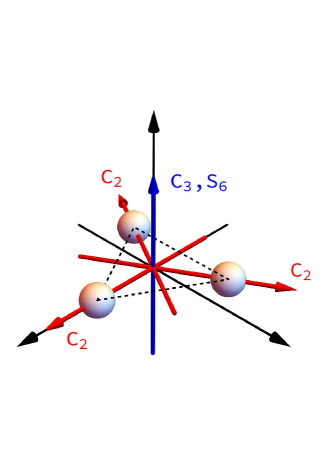
Figure 1: Schematic view of all principal axis and rotation operators for ${\cal D}^{\prime}_{3h}$ symmetry.

To construct a complete wave function we need to understand in more detail the ${\cal D}^{\prime}_{3h}$ symmetry. The objective is to construct a symmetry-adapted basis for ${\cal D}^{\prime}_{3h}$ symmetry instead of a spherical basis[17, 18]. In the case of triangular symmetry the eigenstates of equation 1 can be classified according to the doubly degenerate spinor representations of the double point group ${\cal D}^{\prime}_{3h}$ [19, 20]: $\Omega=E_{1/2}$, $E_{5/2}$ and $E_{3/2}$, or in the notation of Ref. [17] $\Omega=E_{1/2}^{(+)}$, $E_{1/2}^{(-)}$ and $E_{3/2}$, respectively. From similar work in molecular physics, to differentiate between the degenerate states, one finds all rotations of the structure of study; the case in question is shown in figure 1. Then improper rotations are used (in this case the $S_{6}$) to identify the intrinsic states of the doubly degenerate spinor representations. The resulting labels are $\gamma=\pm 5/2$ for $\Omega=E_{5/2}$, $\gamma=\pm 1/2$ for $E_{1/2}$ and $\gamma=\pm 3/2$ for $E_{3/2}$. The Hamiltonian of the CSM is solved in the body-fixed system, using the harmonic oscillator basis $|nljm\rangle$.

$$\phi_{\Omega\gamma}= \sum_{nljm}C^{\Omega\gamma}_{nljm}\left|nljm\right>$$ (6)

The rotational states can be labeled by the angular momentum $I$, parity $P$, and its projection $K$ on the symmetry axis, $|I^{P}K\rangle$. Both $I$ and $K$ are half integers. Then the allowed values of $K^{P}$ for each one of the spinor representations, along with their $\gamma$ labels are given by [17, 18]

$$\begin{array}[]{lcl}\Omega=E_{1/2},\;\gamma=\pm\frac{1}{2}&:&K^{P}=\pm\frac{1}{2}^{+},\mp\frac{5}{2}^{-},\pm\frac{7}{2}^{-},\ldots\\ \Omega=E_{5/2},\;\gamma=\pm\frac{5}{2}&:&K^{P}=\mp\frac{1}{2}^{-},\pm\frac{5}{2}^{+},\mp\frac{7}{2}^{+},\ldots\\ \Omega=E_{3/2},\;\gamma=\pm\frac{3}{2}&:&K^{P}=\pm\frac{3}{2}^{+},\mp\frac{3}{2}^{-},\mp\frac{9}{2}^{+},\ldots\end{array}$$ (10)

with $I=|K|$, $|K|+1$, $\ldots$. A schematic view can be seen in figure 2. The complete wave function is defined then by [18]

$$\left|\Omega\gamma;I^{P}MK\right>=\sqrt{\frac{2I+1}{16\pi^{2}}}\psi_{v}\left(1+{\cal S}_{i}^{-1}{\cal S}_{e}\right)\phi_{\Omega\gamma}D_{MK}^{I}(\omega)$$ (11)

where $\psi_{v}$ is the vibrational wave function, $\phi_{\Omega\gamma}$ the intrinsic wave function and $D_{MK}^{I}(\omega)$ the rotational wave function. The wave function is invariant under the transformation ${\cal S}_{i}^{-1}{\cal S}_{e}$ where the operator ${\cal S}$ is the product of a rotation about $\pi$ followed by a parity transformation [18]. The operator ${\cal S}_{i}^{-1}$ acts on the intrinsic wave function and ${\cal S}_{e}$ on the rotational wave function.

2.3 Splitting of single-particle levels

Previous work on the splitting of single-particle levels is shown in [13, 21]. The splitting of the single-particle energy levels is seen in figure 3. Two simple observations that are illustrated in the figure are that at a value of $\beta=0$ the spherical symmetry is recovered, and at max value, we have 3-fold degeneracy of the spherical symmetry. In other words, at the max value we obtain the view of a particle in a field formed by three separate (not bound in a nucleus) alpha particles, which is unlike the Nilsson model where in the case of max deformation one obtains the splitting for an ”infinite cigar”. From the elastic form factors, one obtains the value for $\beta$ and then comes back to figures 3 and 2 and obtains the base rotational band proposed for ¹³C. Foreshadowing the subsequent section, the value obtained for $\beta$ is 1.71 fm, which in turn gives the ground state rotational band as $\Omega=E_{5/2}$, and the ground state with $I^{P}=\frac{1}{2}^{-}$.

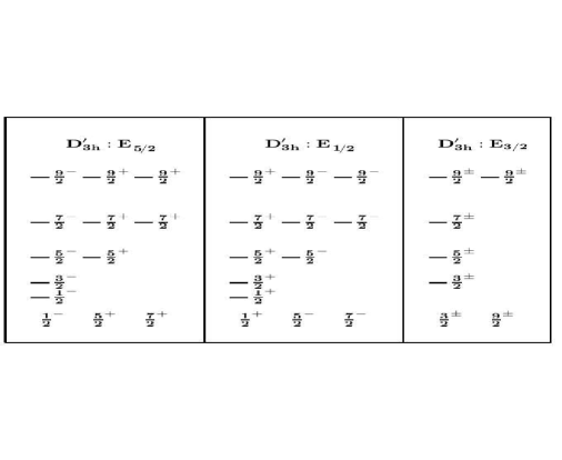
Figure 2: Schematic view of rotational structure with ${\cal D}^{\prime}_{3h}$, proposed for ¹³C. Imagine obtained from [22].

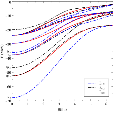
Figure 3: Single-particle energy level splitting from solving equation 1. The values used for equations 3 and 4 are $V_{0}$=32 MeV, $\alpha$=0.0511 fm^-2 and $V_{0,so}$=17 MeV fm^-2.

3 Form Factors and comparison to experimental data

Using equation 11 we can now calculate the form factors for ¹³C and compare them with available experimental data. We use the standard form factors operators, of which a full explanation is found in [23].

3.1 Longitudinal form factors

The charge distribution is taken to be section 2.1, plus a point-like distribution for the extra nucleon

$$\rho(\vec{r})=\frac{(Ze)_{\rm c}}{3}\left(\frac{\alpha}{\pi}\right)^{3/2}\sum_{i=1}^{3}\exp\left[-\alpha\left(\vec{r}-\vec{r}_{i}\right)^{2}\right]+\tilde{e}\delta(\vec{r}-\vec{r}_{\rm sp}),$$ (12)

$(Ze)_{\rm c}$ is the electric charge of the $3\alpha$ core nucleus, and $\tilde{e}$ the effective charge of the extra nucleon, which for the case of ¹³C is taken to be zero. Making a Fourier transformation of equation 12, and then summing over final and averaged over initial states, we obtain the multipoles of the longitudinal (Coulomb) form factor;

$$F_{C\lambda}\left(q;\Omega^{\prime}\gamma^{\prime},I^{\prime}K^{\prime}\rightarrow\Omega\gamma,IK\right) =\frac{\sqrt{4\pi}}{\left(Ze\right)_{\mathrm{odd}}}\langle I^{\prime},K^{\prime},\lambda,K-K^{\prime}\left|I,K\right\rangle\delta_{\Omega\Omega^{\prime}}\delta_{\gamma\gamma^{\prime}}G_{vv^{\prime}}^{\mathrm{c}}\left(q\right),$$ (13)

where $(Ze)_{\rm odd}$ denotes the electric charge of the odd nucleus. For the vibrationally elastic case with $v=v^{\prime}=0$ the collective part is given by

$$G^{\rm c}_{00}(q;\lambda,K-K^{\prime}) =(Ze)_{\rm c}\,j_{\lambda}(q\beta)\,\mbox{e}^{-q^{2}/4\alpha}\,Y_{\lambda,K-K^{\prime}}(\frac{\pi}{2},0)\,\delta_{K-K^{\prime},3\kappa}$$ (14)

A final remark arises when calculating form factors with diagonal intrinsic states. In that case, branching ratios are found between different form factors with the same multipole.

$$\frac{\left|F_{C\lambda}(q;\Omega\gamma,I^{\prime}K^{\prime}\rightarrow\Omega\gamma,I_{1}K_{1})\right|^{2}}{\left|F_{C\lambda}(q;\Omega\gamma,I^{\prime}K^{\prime}\rightarrow\Omega\gamma,I_{2}K_{2})\right|^{2}}=\frac{\left<I^{\prime},K^{\prime},\lambda,K_{1}-K^{\prime}|I_{1},K_{1}\right>^{2}}{\left<I^{\prime},K^{\prime},\lambda,K_{2}-K^{\prime}|I_{2},K_{2}\right>^{2}}.$$ (15)

Finally one sees that the single particle element for Coulomb form factors doesn’t give any contribution to the total value, thus we expect that for both ¹²C and ¹³C to have the same q dependence. The results are illustrated in figures 4 and 5.

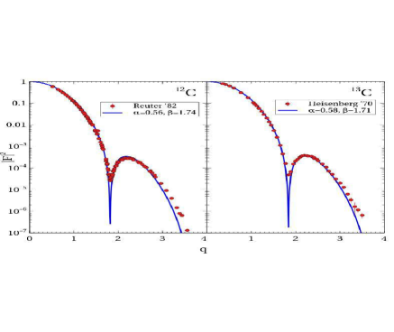
Figure 4: Comparison of elastic form factor between ¹²C (left) and ¹³C(right). Both graphs include available experimental data for both ¹²C[24] and ¹³C[25].

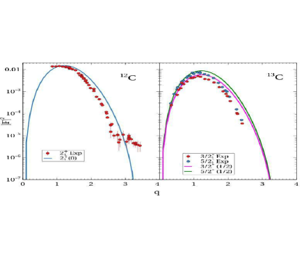
Figure 5: Comparison of C2 form factor between ¹²C (left) and ¹³C(right). Both graphs include available experimental data for both ¹²C[26, 27] and ¹³C[28].

3.2 Transverse form factors

Just as previously done for the Coulomb form factors, the transverse form factors are obtained from a Fourier transform of the current $\vec{J}$ and magnetization operator $\vec{\mu}$, with a little more algebra involved to obtain the final expressions. The main assumption we do from the CSM is that the only contributor to both is the extra nucleon

$$\vec{J} =0$$ (16)

$$\vec{\mu} =\delta\left(\vec{r_{i}}-\vec{x}\right)\mu_{i}\frac{\vec{\sigma}\left(i\right)}{2M_{i}},$$ (17)

where $\mu_{i}$ is the magnetic moment (in nuclear magnetons) of the nucleon involved, in this case for the free neutron is $\mu_{n}=-1.91$ and $M_{i}$ is the mass. The multipoles for the transverse form factor are then given by

$$F_{E\lambda/M\lambda}(q;\Omega^{\prime}\gamma^{\prime},I^{\prime}K^{\prime} =\left<I^{\prime},K^{\prime},\lambda,K-K^{\prime}|I,K\right>\delta_{vv^{\prime}}G_{\Omega\gamma,\Omega^{\prime}\gamma^{\prime}}^{{\rm sp}}(q)$$

$$+P(-1)^{I+K}\left<I^{\prime},K^{\prime},\lambda,-K-K^{\prime}|I,-K\right>\delta_{vv^{\prime}}H_{\Omega\gamma,\Omega^{\prime}\gamma^{\prime}}^{{\rm sp}}(q),$$ (18)

where $G_{\Omega\gamma,\Omega^{\prime}\gamma^{\prime}}^{{\rm sp}}(q)$ and $H_{\Omega\gamma,\Omega^{\prime}\gamma^{\prime}}^{{\rm sp}}(q)$ will have the form

$$G^{\rm sp}_{\Omega\gamma,\Omega^{\prime}\gamma^{\prime}}(q) =\sum_{nljm}\sum_{n^{\prime}l^{\prime}j^{\prime}m^{\prime}}C^{\Omega\gamma}_{nljm}C^{\Omega^{\prime}\gamma^{\prime}}_{n^{\prime}l^{\prime}j^{\prime}m^{\prime}}\left<nljm\left|\hat{T}_{\lambda\mu}^{\zeta}\left(q,\vec{r}\,\right)\right|n^{\prime}l^{\prime}j^{\prime}m^{\prime}\right>$$ (19a)

$$H^{\rm sp}_{\Omega\gamma,\Omega^{\prime}\gamma^{\prime}}(q) =\sum_{nljm}\sum_{n^{\prime}l^{\prime}j^{\prime}m^{\prime}}C^{\Omega\gamma}_{nljm}C^{\Omega^{\prime}\gamma^{\prime}}_{n^{\prime}l^{\prime}j^{\prime}m^{\prime}}(-1)^{n+j+m}\left<nlj,-m\left|\hat{T}_{\lambda\mu}^{\zeta}\left(q,\vec{r}\,\right)\right|n^{\prime}l^{\prime}j^{\prime}m^{\prime}\right>$$ (19b)

and $\hat{T}_{\lambda\mu}^{\zeta}\left(q,\vec{r}\,\right)$ are the electric/magnectic transverse form factor operators

$$\hat{T}_{\lambda\mu}^{E}\left(q,\vec{r}\,\right) =q\frac{\mu_{i}}{2M_{N}}\vec{M}_{\lambda,\lambda}^{\mu}(\vec{r_{i}})\cdot\vec{\sigma}(i)$$

$$\hat{T}_{\lambda\mu}^{M}\left(q,\vec{r}\,\right) =iq\frac{\mu_{i}}{2M_{N}}\left(-\sqrt{\frac{\lambda}{2\lambda+1}}\vec{M}_{\lambda,\lambda+1}^{\mu}(\vec{r_{i}})+\sqrt{\frac{\lambda+1}{2\lambda+1}}\vec{M}_{\lambda,\lambda-1}^{\mu}(\vec{r_{i}})\right)\cdot\vec{\sigma}(i)$$

$$\vec{M}_{\lambda_{1},\lambda_{2}}^{\mu}\left(\vec{r}\,\right) =j_{\lambda_{2}}(qr)\vec{Y}_{\lambda_{1}\lambda_{2}1}^{\mu}(\theta,\phi).$$ (20)

The results are showed in figure 6.

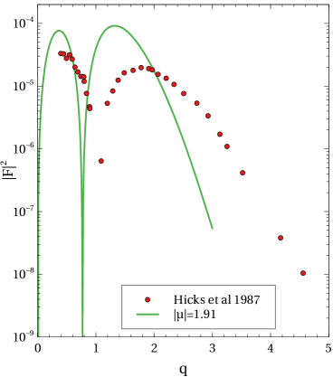
Figure 6: Comparison of M1 elastic form factor between experimental data [28] and CSM calculation.

4 Summary and Conclusions

From calculations, it is seen that for longitudinal form factors in the base rotational band of ¹³C, the cluster core structure is dominant. In those cases, we expected that Coulomb form factors for both ¹²C and ¹³C have the same $q$ dependence. From figures 4 and 5 we see that the experimental data seems to support that idea, differing only slightly in some aspects. Also, it shows for ¹³C that longitudinal form factors follow a branching ratio rule like the one in equation 15. This is of great importance since it indicates that some properties of the cluster structure in ¹²C are still present in ¹³C.

Unfortunately, such a positive outcome was not the case for the transverse form factors. From figure 6 we are not able to reproduce available experimental data. Only global functional properties are reproduced of [28]. It is most likely that our assumptions in equations 16 and 17 are incorrect and must then include a contribution of the cluster core. A possible solution may be found in [29], but it would have to be adapted for the CSM.

To reiterate, the CSM as is now is a good approximation to calculate longitudinal form factors for ¹³C, reproducing accurately the available experimental data. Meanwhile, in the case of transverse form factors, the model is still lacking, due most likely to not considering the contribution of the cluster structure to the transverse form factors.

This work was supported in part by research grants IN101320, IG101423 from PAPIIT-DGAPA and 784896 from CONACYT.

References

References

• [1] Wheeler J A 1937 Phys. Rev. 52 1083–1106
• [2] Hafstad L R and Teller E 1938 Phys. Rev. 54 681–692
• [3] Brink D 1965 Int. School of Physics Enrico Fermi (Varenna, 1965) 247
• [4] Brink D, Friedrich H, Weiguny A and Wong C 1970 Phys. Lett. B 33 143–146
• [5] Kanada-En’yo Y 2007 Prog. Theor. Phys. 117 655–680
• [6] Chernykh M, Feldmeier H, Neff T, von Neumann-Cosel P and Richter A 2007 Phys. Rev. Lett. 98 032501
• [7] Funaki Y, Horiuchi H, von Oertzen W, Röpke G, Schuck P, Tohsaki A and Yamada T 2009 Phys. Rev. C 80 064326
• [8] Epelbaum E, Krebs H, Lee D and Meißner U G 2011 Phys. Rev. Lett. 106 192501
• [9] Bijker R and Iachello F 2002 Ann. Phys. 298 334–360
• [10] Freer M and Fynbo H 2014 Prog. Part. Nucl. Phys. 78 1–23
• [11] Schuck P, Funaki Y, Horiuchi H, Röpke G, Tohsaki A and Yamada T 2016 Phys. Scr. 91 123001
• [12] Freer M, Horiuchi H, Kanada-En’yo Y, Lee D and Meißner U G 2018 Rev. Mod. Phys. 90 035004
• [13] Della Rocca V, Bijker R and Iachello F 2017 Nucl. Phys. A 966 158–184
• [14] Della Rocca V and Iachello F 2018 Nucl. Phys. A 973 1–32
• [15] Bijker R and Iachello F 2020 Prog. Part. Nucl. Phys. 110 103735
• [16] Nilsson S G 1955 Kong. Dan. Vid. Sel. Mat. Fys. Med. 29 1–69
• [17] Bijker R and Iachello F 2019 Phys. Rev. Lett. 122 162501
• [18] Santana Valdés A H and Bijker R 2020 Eur. Phys. J. ST 229 2353–2366
• [19] Herzberg G 1991 Electronic Spectra and Electronic Structure of Polyatomic Molecules (Molecular spectra and molecular structure vol II) (Malabar, Fla: R.E. Krieger Pub. Co.) ISBN 0894642685
• [20] Koster G F, Dimmock J O, Wheeler R G and Statz H 1963 Properties of the thirty-two point groups vol 24 (MIT press Cambridge, MA)
• [21] Santana-Valdés A and Bijker R 2018 J. Phys. Conf. Ser. 1078 012019
• [22] Bijker R and Santana-Valdés A 2020 Journal of Physics: Conference Series 1643 012113
• [23] de Forest T and Walecka J 1966 Adv. Phys. 15 1–109
• [24] Reuter W, Fricke G, Merle K and Miska H 1982 Phys. Rev. C 26 806–818
• [25] Heisenberg J, McCarthy J and Sick I 1970 Nucl. Phys. A 157 435–448
• [26] Crannell H L and Griffy T A 1964 Phys. Rev. 136 B1580–B1584
• [27] Crannell H 1966 Phys. Rev. 148 1107–1118
• [28] Millener D J, Sober D I, Crannell H, O’Brien J T, Fagg L W, Kowalski S, Williamson C F and Lapikás L 1989 Phys. Rev. C 39 14–46
• [29] Delorme J, Figureau A and Guichon P 1981 Physics Letters B 99 187–190