On the area of optimal parameters choice for the numerical method of non-stationary hydrodynamics problem with feature

Abstract

For an approximate solution of the non-stationary nonlinear Navier-Stokes equations for the flow of an incompressible viscous fluid, depending on the set of input data and the geometry of the domain, the area of optimal parameters in the variables $\nu$ and $\nu^{\ast}$ is experimentally determined depending on $\delta$ included in the definition of the $R_{\nu}$-generalized solution of the problem and the degree of the weight function in the basis of the finite element method. To discretize the problem in time, the Runge-Kutta methods of the first and second orders were used. The areas of optimal parameters for various values of the incoming angles are established. Keywords: nonlinear Navier-Stokes equations, feature, finite element method.

Computing Center of the Far Eastern Branch of the Russian Academy of Sciences,

680000, Khabarovsk, Russia, e-mail: 78321a@mail.ru

Introduction.

The purpose of this study is to find the area of optimal parameters choice for the numerical method of non-stationary Navier-Stokes equations with feature. The search for a solution to a nonlinear problem is reduced to a sequence of approximate linear problems using Runge-Kutta methods of 1st and 2nd order. The peculiarity of the study lies in the fact that the domain is a non-convex polygon with a incoming angle at the boundary. Using classical approximate methods, the error arising in the vicinity of the feature point propagates into the inner part of the domain, where the solution has sufficient smoothness. In this case, the convergence rate of the approximate solution to the exact one is significantly less than for convex domains. The proposed numerical method overcomes these difficulties. It is based on two ideas, namely, the introduction into the variational formulation of problems a weight function to some order and special basis functions.

In [1] the concept of an $R_{\nu}$-generalized solution in weighted sets for the Stokes problem is defined. The main feature of the variational formulation of this problem, in contrast to the classical formulation [2], is that it is asymmetrical. In [3] the existence and uniqueness of an $R_{\nu}$-generalized solution for the Stokes problem is established.

In the course of numerical experiments, an area of optimal parameters of the method was determined. The order of convergence of the approximate solution to the exact one of the nonlinear problem is the same for angles more than $\pi$ and significantly greater than using classical approaches. Part of the optimal set of free parameters of the proposed method doesn’t depend on the value of the incoming angle. The optimal convergence rate is achieved without using a mesh refinement in the vicinity of the feature point.

1. The problem statement.

Consider the flow of a viscous incompressible fluid in a 2-dimensional non-convex polygonal domain $\Omega$ with an incoming angle $\omega$ on its boundary $\partial\Omega$ with a vertex at the origin ${\cal O}=(0,0)$. Let ${\bf x}=(x_{1},x_{2})$ be an element in $R^{2},$ $t$ be an element in time and $Q=\Omega\times(0,T)$. Given fields ${\bf u}_{0}={\bf u}_{0}({\bf x})$ in $\Omega,{\bf f}={\bf f}({\bf x},t)=\{f_{i}({\bf x},t)\}_{i=1}^{2}$ in $Q$ and ${\bf g}={\bf g}({\bf x},t)=\{g_{i}({\bf x},t)\}_{i=1}^{2}$ in $Q$ such that $\int\limits_{\Omega}{\mbox{div}\,{\bf g}d{\bf x}}=0$ at each time $t\in(0,T),$ it is required to find the fields ${\bf u}={\bf u}({\bf x},t)=\{u_{i}({\bf x},t)\}_{i=1}^{2}$ and $P=P({\bf x},t)$ such that the following identities hold:

$$\frac{\partial{\bf u}}{\partial t}-\triangle{\bf u}+\mbox{ curl }{\bf u}\times{\bf u}+\mbox{ grad }P={\bf f},\qquad\,\,\mbox{ div }{\bf w}={0}\,\qquad\mbox{ in }\,\,\qquad Q,$$ (1)

$$\qquad\qquad\,\,\,\,\,{\bf u}({\bf x},0)={\bf u}_{0}\qquad\mbox{ in }\qquad\Omega,\qquad\qquad{\bf u}={\bf g}\qquad\mbox{ on }\qquad\partial\Omega\times(0,T).$$ (2)

As a time discretization of problem (1)-(2), we use the Runge-Kutta schemes of the 1st and 2nd orders. To do this, we first introduce the notation ${\bf v}^{n}={\bf v}^{n}({\bf x})$ to approximate the function ${\bf v}({\bf x},n\triangle t),n=0,1,2,...,N$ and ${\bf v}^{n+\gamma}$ to approximate the function ${\bf v}({\bf x},(n+\gamma)\triangle t),\gamma\in(0,1),n=0,1,2,...,N-1$. Parameter $\triangle t$ is such that $T=N\cdot\triangle t.$ Moreover, let ${\bf v}^{-1}:={\bf v}^{0}$ and $\bar{\bf v}^{n+1}:=0.5({\bf v}^{n+1}+{\bf v}^{n})$ and ${\bf U}^{n}$ a suitable approximation to u at time $n\triangle t.$

1st order scheme.

Given ${\bf u}^{n},{\bf U}^{n}:=\frac{3}{2}{\bf u}^{n}-\frac{1}{2}{\bf u}^{n-1},P^{n},\bar{\bf f}^{n+1}$ and ${\bf g}^{n+1}$: find ${\bf u}^{n+1}$ and $P^{n+1}$ as a solution to the system of equations:

$$(\triangle t)^{-1}{\bf u}^{n+1}-\triangle\bar{\bf u}^{n+1}+\mbox{ curl }{\bf U}^{n}\times\bar{\bf u}^{n+1}+\mbox{ grad }\bar{P}^{n+1}=\bar{\bf f}^{n+1}+(\triangle t)^{-1}{\bf u}^{n}\qquad\mbox{ in }\,\,\qquad\Omega,$$ (3)

$$\qquad\qquad\qquad\qquad\qquad\qquad\qquad\qquad\qquad\qquad\qquad\qquad\qquad\,\,\mbox{ div }{\bf u}^{n+1}={0}\,\qquad\mbox{ in }\,\,\qquad\Omega,$$ (4)

$$\qquad\qquad\qquad\qquad\qquad\qquad\qquad\qquad\qquad\qquad\qquad\qquad\qquad\qquad{\bf u}^{n+1}={\bf g}^{n+1}\qquad\mbox{ on }\qquad\partial\Omega.$$ (5)

2nd order scheme.

This scheme consists of two steps.

Step 1.

Given ${\bf u}^{n},{\bf U}^{n}:=\frac{3}{2}{\bf u}^{n}-\frac{1}{2}{\bf u}^{n-1},{\bf f}^{n+\gamma}$ and ${\bf g}^{n+\gamma}$: find ${\bf u}^{n+\gamma}$ and $P^{n+\gamma}(\gamma\in(0,1))$ as a solution to the system of equations:

$$(\gamma\triangle t)^{-1}{\bf u}^{n+\gamma}-\triangle{\bf u}^{n+\gamma}+\mbox{ curl }{\bf U}^{n}\times{\bf u}^{n+\gamma}+\mbox{ grad }P^{n+\gamma}={\bf f}^{n+\gamma}+(\gamma\triangle t)^{-1}{\bf u}^{n}\qquad\mbox{ in }\,\,\qquad\Omega,$$ (6)

$$\qquad\qquad\qquad\qquad\qquad\qquad\qquad\qquad\qquad\qquad\qquad\qquad\qquad\,\,\mbox{ div }{\bf u}^{n+\gamma}={0}\,\qquad\mbox{ in }\,\,\qquad\Omega,$$ (7)

$$\qquad\qquad\qquad\qquad\qquad\qquad\qquad\qquad\qquad\qquad\qquad\qquad\qquad\qquad{\bf u}^{n+\gamma}={\bf g}^{n+\gamma}\qquad\mbox{ on }\qquad\partial\Omega.$$ (8)

Step 2.

Given ${\bf u}^{n},{\bf u}^{n+\gamma},P^{n+\gamma},{\bf U}^{n}:=\frac{3}{2}{\bf u}^{n}-\frac{1}{2}{\bf u}^{n-1},{\bf f}^{n+1},{\bf f}^{n+\gamma}$ and ${\bf g}^{n+1}$: find ${\bf u}^{n+1}$ and $P^{n+1}$ as a solution to the system of equations:

$$(\triangle t)^{-1}{\bf u}^{n+1}+\gamma(-\triangle{\bf u}^{n+1}+\mbox{ curl }{\bf U}^{n}\times{\bf u}^{n+1}+\mbox{ grad }P^{n+1})=$$ (9)

$$=(\triangle t)^{-1}{\bf u}^{n}+\gamma{\bf f}^{n+1}+(1-\gamma){\bf f}^{n+\gamma}-(1-\gamma)(-\triangle{\bf u}^{n+\gamma}+\mbox{ curl }{\bf U}^{n}\times{\bf u}^{n+\gamma}+\mbox{ grad }P^{n+\gamma})\quad\mbox{ in }\quad\Omega,$$

$$\qquad\qquad\qquad\qquad\qquad\qquad\qquad\qquad\qquad\qquad\qquad\qquad\qquad\qquad\,\,\mbox{ div }{\bf u}^{n+1}={0}\,\qquad\mbox{ in }\,\,\qquad\Omega,$$ (10)

$$\qquad\qquad\qquad\quad\qquad\qquad\qquad\qquad\qquad\qquad\qquad\qquad\qquad\qquad\qquad{\bf u}^{n+1}={\bf g}^{n+1}\qquad\mbox{ on }\qquad\partial\Omega.$$ (11)

At each step of both schemes, it is necessary to be able to solve the following problem: find the fields ${\bf v}=(v_{1},v_{2})$ and $q$ such that

$$\theta{\bf v}-\triangle{\bf v}+W\times{\bf v}+\mbox{ grad }q={\bf F}\qquad\mbox{ in }\,\,\qquad\Omega,$$ (12)

$$\qquad\qquad\qquad\qquad\qquad\,\,\mbox{ div }{\bf v}={0}\,\qquad\mbox{ in }\,\,\qquad\Omega,$$ (13)

$$\qquad\qquad\qquad\qquad\qquad\qquad{\bf v}={\bf G}\qquad\mbox{ on }\qquad\partial\Omega,$$ (14)

where ${\bf F}$ and $W$ are given functions on $\Omega$ and ${\bf G}$ is given on $\partial\Omega.$

Let us define an $R_{\nu}$-generalized solution of problem (12)-(14) in the domain $\Omega,$ having an incoming angle on the $\partial\Omega$ with a vertex at the origin. To do this, we define the necessary weight sets. First, we introduce the concept of a weight function $\rho({\bf x}):\rho({\bf x})=\{\sqrt{x_{1}^{2}+x^{2}_{2}},\mbox{ if }{\bf x}\in\Omega_{\delta}\mbox{ and }\delta,\mbox{ if }{\bf x}\in\bar{\Omega}\diagdown\Omega_{\delta}\},$ where $\Omega_{\delta}=\{{\bf x}\in\bar{\Omega}:\sqrt{x_{1}^{2}+x^{2}_{2}}\leq\delta\}$ and $\delta\ll 1.$

Denote by $L_{2,\alpha}(\Omega,\delta)$ the set of functions $s({\bf x})$ satisfying the conditions:
1) $\|\rho^{\alpha}s\|_{L_{2}(\Omega\diagdown\Omega_{\delta})}\geq C_{1}>0;$
2) $|s({\bf x})|\leq C_{2}\delta^{\alpha-\varepsilon}\rho^{\varepsilon-\alpha}({\bf x}),{\bf x}\in\Omega_{\delta},$
where $C_{2}$ is a positive constant independents $s({\bf x})$, $\varepsilon$ is a small positive parameter independent of $\delta,\alpha,s({\bf x}),$ with bounded norm $\|s\|_{L_{2,\alpha}(\Omega)}:=\|\rho^{\alpha}s\|_{L_{2}(\Omega)}$ of the space $L_{2,\alpha}(\Omega).$ $L^{0}_{2,\alpha}(\Omega,\delta)$ subset of $L_{2,\alpha}(\Omega)$ such that $s\in L^{0}_{2,\alpha}(\Omega,\delta),$ if $s\in L_{2,\alpha}(\Omega)$ and $\|\rho^{\alpha}s\|_{L_{1}(\Omega)}=0.$

Denote by $W^{1}_{2,\alpha}(\Omega,\delta)$ the set of functions $s({\bf x})$ satisfying the conditions:
1) $\|\rho^{\alpha}s\|_{L_{2}(\Omega\diagdown\Omega_{\delta})}\geq C_{1}>0;$
2) $|s({\bf x})|\leq C_{2}\delta^{\alpha-\varepsilon}\rho^{\varepsilon-\alpha}({\bf x}),{\bf x}\in\Omega_{\delta},$
3) $|D^{1}s({\bf x})|\leq C_{2}\delta^{\alpha-\varepsilon}\rho^{\varepsilon-\alpha-1}({\bf x}),{\bf x}\in\Omega_{\delta},$
where $C_{2}$ is a positive constant independent $s({\bf x})$, $\varepsilon$ is a small positive parameter, independent of $\delta,\alpha,s({\bf x}),$ with bounded norm $\|s\|_{W^{1}_{2,\alpha}(\Omega)}:=\sqrt{\sum\limits_{|k|\leq 1}{\|\rho^{\alpha}|D^{k}s|\|^{2}_{L_{2}(\Omega)}}}$ of the space $W^{1}_{2,\alpha}(\Omega).$ $\hat{W}^{1}_{2,\alpha}(\Omega,\delta)$ subset $W^{1}_{2,\alpha}(\Omega)$ such that $s\in\hat{W}^{1}_{2,\alpha}(\Omega,\delta),$ if $s\in W^{1}_{2,\alpha}(\Omega,\delta)$ and $s=0$ on $\partial\Omega.$

Let $L_{\infty,\alpha}(\Omega,C_{3})$ be the set of functions $s({\bf x})$ with a norm $\|s\|_{L_{\infty,\alpha}(\Omega,C_{3})}=\mbox{vrai}\max\limits_{{\bf x}\in\Omega}{|\rho^{\alpha}({\bf x})s({\bf x})|}\leq C_{3},$ where $C_{3}>0$ independent of $s({\bf x})$.

Let us define an $R_{\nu}$-generalized solution of problem (12)-(14).

Definition 1. Pair $({\bf v}_{\nu},q_{\nu})\in{\bf W}^{1}_{2,\nu}(\Omega,\delta)\times L^{0}_{2,\nu}(\Omega,\delta)$ is called $R_{\nu}$-generalized solution of problem (12)-(14) if ${\bf w}_{\nu}$ satisfies (14) on $\partial\Omega$ and identities

$$a({\bf v}_{\nu},{\bf z})+b({\bf z},q_{\nu})=l({\bf z}),$$ (15)

$$c({\bf v}_{\nu},s)=0\qquad\qquad\qquad$$ (16)

hold, for all $({\bf z},s)\in\hat{\bf W}^{1}_{2,\nu}(\Omega,\delta)\times L^{0}_{2,\nu}(\Omega,\delta)$. Here $({\bf F},W,{\bf G})\in{\bf L}_{2,\alpha}(\Omega,\delta)\times L_{\infty,\beta}(\Omega,C_{3})\times{\bf W}^{1/2}_{2,\alpha}(\partial\Omega,\delta),\nu\geq\alpha\geq 0,\beta\leq 2.$

We have $a({\bf w},{\bf z})=\int\limits_{\Omega}{\Bigl{[}\theta{\bf w}\cdot(\rho^{2\nu}{\bf z})+\nabla{\bf w}:\nabla(\rho^{2\nu}{\bf z})+(W\times{\bf w})\cdot(\rho^{2\nu}{\bf z})\Bigr{]}d{\bf x}},$
$b({\bf z},p)=-\int\limits_{\Omega}{p\mbox{ div }(\rho^{2\nu}{\bf z})}d{\bf x},\,\,\,c({\bf w},s)=-\int\limits_{\Omega}{(\rho^{2\nu}s)\mbox{ div }{\bf w}}d{\bf x},\,\,\,l({\bf z})=\int\limits_{\Omega}{{\bf F}\cdot(\rho^{2\nu}{\bf z})}d{\bf x}.$

Remark 1. $b(\cdot,\cdot)\neq c(\cdot,\cdot)$. Consequently, the variational problem (15), (16) is not symmetric, in contrast to the standard setting (see [2]).

Remark 2. If $W\in L_{\infty,\beta}(\Omega,C_{3}),\beta\leq 2,{\bf g=0}$ on $\partial\Omega,$ then there exists a unique $R_{\nu}$-generalized solution $({\bf w}_{\nu},q_{\nu})$ problem (12)-(14) in the asymmetric formulation (15), (16) (see Theorem 5 in [5]).

Remark 3. Scheme 2 (6)-(11) can be applied when $\gamma$ equal to $1-\frac{\sqrt{2}}{2}$ (strongly L-stable method [4]). Scheme 1 can be applied due to the validity of Theorem 6 [5].

2. Creation of an approximate approach.

We will build a quasi-uniform fragmentation $I^{h}$ of the domain $\bar{\Omega}$ into triangles $K_{i}$. Their sides of order $h$ which are the essential elements. We split each of them into 3 using the center of mass, which are finite elements $L_{i_{j}}$ that make up the fragmentation $J^{h}$.

We define the main finite element spaces.

1. For the velocity components. We will use Lagrangian elements of the 2nd order with nodes at the vertices and midpoints of the sides of $L_{i_{j}}$. The linear span of basic functions $\chi_{k}({\bf x})$ will be denote by $W_{h}$.

2. For the pressure. As approximation nodes, we use the vertices of finite elements, and the vertices of neighboring finite elements are different nodes. On each $L_{i_{j}}$ we define 1st order basis functions $\theta_{l}({\bf x})$ whose support is only one finite element. The linear span of such basis functions forms a space $S_{h}$, consisting of functions discontinuous in the domain under consideration.

The pair ${\bf W}_{h}\times S_{h}({\bf W}_{h}=W_{h}\times W_{h})$ is a Scott-Vogelius 2nd order one [6].

Let’s multiply the basis functions of the spaces $W_{h}$ and $S_{h}$ by the weight function $\rho({\bf x})$ in some powers ($-\nu^{\ast}$) and (-$\mu^{\ast}$). The values of the powers will be determined later. We define new basis functions $\phi_{k}({\bf x})=\chi_{k}({\bf x})\cdot\rho^{-\nu^{\ast}}({\bf x}),\psi_{l}({\bf x})=\theta_{l}({\bf x})\cdot\rho^{-\mu^{\ast}}({\bf x})$.

Their linear spans form finite-dimensional spaces $V_{h}$ and $Q_{h}$ respectively. $\hat{V}_{h}=\{u_{h}\in V_{h}:u_{h}(M_{i})=0\mbox{ where }M_{i}\mbox{ are nodes on }\partial\Omega\}$. Having found the solution $\hat{v}_{i}$ and $\hat{q}_{j}$ at the nodes $M_{i}$ and $N_{j}$ for the velocity components and pressure of system of equations (presented below) it is necessary to restore the true values at the nodes $M_{i}$ and $N_{j}$ using the formulas $v_{i}=\hat{v}_{i}\cdot\rho^{-\nu^{\ast}}(M_{i})$ and $q_{j}=\hat{q}_{j}\cdot\rho^{-\mu^{\ast}}(N_{j}).$ We have ${\bf V}_{h}=V_{h}\times V_{h}\subset{\bf W}^{1}_{2,\nu}(\Omega,\delta),\hat{\bf V}_{h}=\hat{V}_{h}\times\hat{V}_{h}\subset\hat{\bf W}^{1}_{2,\nu}(\Omega,\delta),Q_{h}\subset L^{0}_{2,\nu}(\Omega,\delta).$

We are all set to determine an approximate $R_{\nu}$-generalized solution of the problem (12)-(14).

Definition 2. We will say that a pair of functions $({\bf v}^{h}_{\nu},\,q^{h}_{\nu})$ from the spaces ${\bf V}_{h}\times Q_{h},$ satisfying condition (14) at the nodes on $\partial\Omega$, is an approximate $R_{\nu}$-generalized solution of the problem (12)-(14) if for all pairs of functions $({\bf z}^{h},s^{h})$ from the spaces $\hat{\bf V}_{h}\times Q_{h}$ the following relations

$$a({\bf v}^{h}_{\nu},{\bf z}^{h})+b({\bf z}^{h},q^{h}_{\nu})=l({\bf z}^{h}),$$ (17)

$$c({\bf v}^{h}_{\nu},s^{h})=0\qquad\quad\,\,\,\qquad\quad$$ (18)

hold.

Remark 4.

How to solve the system (17), (18) by the iterative method see [7].

Remark 5.

If $\nu=\nu^{\ast}=\mu^{\ast}=0$ then we have an approximate generalized solution $({\bf v}^{h},\,q^{h})$ of the problem (12)-(14).

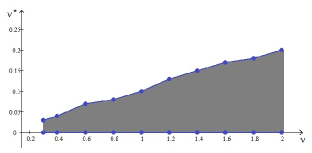
Figure 1: Optimal parameters of the weighted FEM for $(\nu,\nu^{\ast}),\delta\in[0.025,0.035],\omega=\frac{9\pi}{8}$.

3. The results of numerical experiments.

Let’s carry out a number of numerical experiments to find an approximate solution to problem (1)-(2) as a sequence of solving problem (12)-(14) of both formulation schemes (17)-(18). Consider domains $\Omega_{k},k=1,2,3$ with incoming angle $\omega_{k},$ where

$$\Omega_{0}=\{(x_{1},x_{2}):-1<x_{1}<1,0<x_{2}<1\},$$

$$\bar{\Omega}_{1}=\bar{\Omega}_{0}\cup\{(x_{1},x_{2}):-1\leq x_{1}\leq 0,-1\leq x_{2}\leq 0\},$$

$$\bar{\Omega}_{2}=\bar{\Omega}_{0}\cup\{(x_{1},x_{2}):-1\leq x_{1}\leq 0,x_{1}\leq x_{2}\leq 0\},$$

$$\bar{\Omega}_{3}=\bar{\Omega}_{0}\cup\{(x_{1},x_{2}):-1\leq x_{1}\leq 0,\frac{1}{2}x_{1}\leq x_{2}\leq 0\}.$$

In such cases $\omega_{k}=(1+2^{-k})\pi,k=1,2,3.$

Denote by ${\bf u}^{h_{i}}_{\nu}$ and ${\bf u}^{h_{i}}$ an approximate $R_{\nu}$-generalized and generalized solutions (velocity field) of the solution of the problem (1)-(2) at each moment of time. In the second case $(\nu=\nu^{\ast}=\mu^{\ast}=0,\delta=1).$ In the first case $(\nu,\nu^{\ast},\mu^{\ast},\delta)$ is the set of free parameters of the weighted finite element method.

The exact solution of the problem (1)-(2) of the velocity and pressure fields depend on the value of the incoming angle $\omega_{k}$ in each moment of time do not belong to the spaces ${\bf W}^{2}_{2}(\Omega_{k})$ and ${\bf W}^{1}_{2}(\Omega_{k})$, respectively, and have the form in polar coordinates $(r,\theta):$
$u_{1}(r,\theta,t)=e^{t}\Bigl{(}r^{\lambda_{k}}\chi_{1}(\theta)+\psi_{1}(r,\theta)\Bigr{)},$ $u_{2}(r,\theta,t)=e^{t}\Bigl{(}r^{\lambda_{k}}\chi_{2}(\theta)+\psi_{2}(r,\theta)\Bigr{)},$ $P(r,\theta,t)=e^{t}r^{\lambda_{k}-1}\gamma(\theta),$
where $\psi_{i}(r,\theta)$ is the regular part of $u_{i}(r,\theta,t),$ i.e. a function belonging to the space ${\bf W}^{2}_{2}(\Omega_{k}),$ and $r^{\lambda_{k}}\chi_{i}(\theta)$ and $r^{\lambda_{k}-1}\gamma(\theta)$ are the singular solution parts of the velocity and pressure fields. The exponent $\lambda_{k}$ is such that it coincides with the smallest real positive solution of the equation $\sin(\lambda\omega_{k})+\lambda\sin\omega_{k}=0$. Thus $(\lambda_{1},\lambda_{2},\lambda_{3})$ take the following approximate values $(0.5445,0.6736,0.8008).$

We have

$$\chi_{1}(\theta)=\cos(\theta)\,\Xi^{\prime}_{k}(\theta)+(1+\lambda_{k})\,\sin(\theta)\,\Xi_{k}(\theta),$$

$$\chi_{2}(\theta)=(\lambda_{k}-1)\,\cos(\theta)\,\Xi_{k}(\theta)+\sin(\theta)\,\Xi^{\prime}_{k}(\theta),$$

$$\gamma(\theta)=(\lambda_{k}-1)^{-1}\,\Bigl{(}\Xi^{\prime\prime\prime}_{k}(\theta)+(1+\lambda_{k})^{2}\,\Xi^{\prime}_{k}(\theta)\Bigr{)}.$$

Here

$$\Xi_{k}(\theta)=\Bigl{[}(1+\lambda_{k})^{-1}\sin((1+\lambda_{k})\theta)-(1-\lambda_{k})^{-1}\sin((1-\lambda_{k})\theta)\Bigr{]}\cos(\lambda_{k}\omega_{k})+\cos((1-\lambda_{k})\theta)-\cos((1+\lambda_{k})\theta),$$

$\Xi^{\prime}_{k}(\theta)$ and $\Xi^{\prime\prime\prime}_{k}(\theta)$ are its the first and third derivatives with respect to $\theta$, respectively.

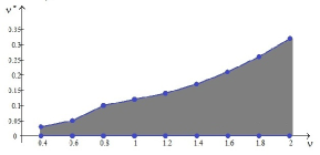
Figure 2: Optimal parameters of the weighted FEM for $(\nu,\nu^{\ast}),\delta\in[0.025,0.035],\omega=\frac{5\pi}{4}$.

In test cases, consider different steps $h_{j}=2^{1-j}\cdot h,h=0.025,j=1,2,3.$ Time step $\triangle t=0.01,T=0.5.$ Shown earlier as for stationary [8] and non-stationary problems [5] problems, it is possible to determine sets of optimal parameters for which the order of convergence of the approximate solution to exact solution is equal to ${\cal O}(h),$ independent of the incoming angle $\omega_{k}$ in the norm ${\bf W}^{1}_{2,\nu}(\Omega_{k}).$ To determine the range of choice of optimal approach parameters, we fix the range $\delta\sim h_{1}:\delta\in[0.025,0.035].$ Let $\nu^{\ast}=\mu^{\ast}$ and will take non-negative values. Moreover, each $\omega_{k}$ will have its own range of value change. The parameter $\nu$ is positive and not exceed the value 2.

For the first scheme, consider the case

$$\psi_{1}(r,\theta)=\psi_{2}(r,\theta)=0$$

(the solution contains only singular components).

For the second scheme

$$\psi_{1}(r,\theta)=\sin(r\cos(\theta))\cdot\cos(r\cos(\theta)),\psi_{2}(r,\theta)=-\cos(r\cos(\theta))\cdot\sin(r\sin(\theta)).$$

We will assume that the set $(\nu^{\ast},\nu)$ falls into the area of choice of optimal parameters of the numerical method for solving problem (1)-(2), if it differs by no more than 5 percent from the optimal value in terms of convergence in each moment of time for all $h_{j},j=1,2,3.$ The Figures 1-3 show the area of choice of optimal parameters in the corresponding ranges for the first scheme for all values of the angle $\omega_{k},k=1,2,3.$ For the second scheme, the results similar in structure.

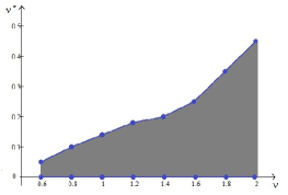
Figure 3: Optimal parameters of the weighted FEM for $(\nu,\nu^{\ast}),\delta\in[0.025,0.035],\omega=\frac{3\pi}{2}$.

Conclusions.

It is also necessary to investigate other values of the incoming angle $\omega$ and determine the intersection areas of choice the optimal parameters of the method for each $\omega$. In order to establish the area of optimal parameters of the method for which the required order of convergence is guaranteed regardless of the incoming angle value.

References

[1]Rukavishnikov V.A., Rukavishnikov A.V.
Weighted finite element method for the Stokes problem
with corner singularity.
J. Comput. Appl. Math.
2018; 341:144–156. DOI: 10.1016/j.cam.2018.04.014.
[2]Brezzi F., Fortin M.
Mixed and hybrid finite element methods.
New York: Springer-Verlag; 1991: 350.
[3]Rukavishnikov V.A., Rukavishnikov A.V.
On the existence and uniqueness of an -generalized solution
to the Stokes problem with corner singularity.
Mathematics. 2022; 10(10): 1752.
DOI: 10.3390/math10101752.
[4]Alexander R.
Diagonally implicit Runge-Kutta methods for stiff odes. SIAM J. Numer. Anal., 1977; 14: 1006–1021.
[5]Rukavishnikov V.A., Rukavishnikov A.V.
Theoretical analysis and construction of numerical method for solving the Navier-Stokes equations in rotation form with corner singularity. J. Comput. Appl. Math., 2023; 429: 115218.
[6]Scott L.R. and Vogelius M.
Norm estimates for a maximal right inverse of the divergence operator
in spaces of piecewise polynomials. Mathematical Modeling and Numerical Analysis, 1985; 19: 111–143.
[7]Rukavishnikov A.V.
On the optimal set of parameters for an approximate method for solving stationary nonlinear Navier-Stokes equations with singularity. Computational Technologies, 2022; 27(6): 70–87.
[8]Rukavishnikov A.V.
A numerical approach for solving one nonlinear problem of hydrodynamics in a non-convex polygonal domain.
Computational Continuum Mechanics, 2022; 15(1): 19–30.