Joint Communication and Computation Framework for Goal-Oriented Semantic Communication with Distortion Rate Resilience

Abstract

Recent research efforts on semantic communication have mostly considered accuracy as a main problem for optimizing goal-oriented communication systems. However, these approaches introduce a paradox: the accuracy of artificial intelligence (AI) tasks should naturally emerge through training rather than being dictated by network constraints. Acknowledging this dilemma, this work introduces an innovative approach that leverages the rate-distortion theory to analyze distortions induced by communication and semantic compression, thereby analyzing the learning process. Specifically, we examine the distribution shift between the original data and the distorted data, thus assessing its impact on the AI model’s performance. Founding upon this analysis, we can preemptively estimate the empirical accuracy of AI tasks, making the goal-oriented semantic communication problem feasible. To achieve this objective, we present the theoretical foundation of our approach, accompanied by simulations and experiments that demonstrate its effectiveness. The experimental results indicate that our proposed method enables accurate AI task performance while adhering to network constraints, establishing it as a valuable contribution to the field of signal processing. Furthermore, this work advances research in goal-oriented semantic communication and highlights the significance of data-driven approaches in optimizing the performance of intelligent systems.

I Introduction

The rapidly advancing sixth generation (6G) communication technology is enabling the transition from serving individual users and devices towards underpinning the expansive Internet of Everything (IoE) [1, 2]. Specifically, 6G communication technology orchestrates the seamless integration of humans, machines, and objects, fostering intelligent cooperation and synergy, and actively catalyzing the development of an inclusive and intelligent human society [3]. However, the traditional point-to-point information transmission systems, that relies on the resource optimization of physical layer and the stable transmission protocol at the network layer, cannot meet the increasing demands for complex, diverse, and intelligent information transmission. This includes the provision of support for emerging applications like virtual reality, holographic projection, and Metaverse [4]. Consequently, it becomes imperative to devise a novel communication paradigm for efficient information transmission thereby aligning with the evolving requisites of future wireless communication applications.

Fortunately, Semantic Communication (SemCom) [5, 6, 7, 8] emerges as a promising architectural innovation poised to redefine communication in the IoE era. The SemCom system’s ultimate objective is the efficient transmission of content-aware and semantic-related information tailored to specific tasks, thus bringing the grand vision of the IoE closer to reality. Achieving this requires core feature: the semantic receiver’s capability to reconstruct the original data, accepting a degree of distortion as long as it surpasses a predefined AI task performance threshold. To this end, various studies have introduced goal-oriented SemCom approaches that leverages semantic features (e.g., semantic similarity, semantic completeness, and semantic accuracy) to ensure effective AI task execution within the constraints of wireless communication environments. For instance, in [9], the authors proposed DeepSC, which employs semantic channel coding for text transmission. It maximizes data rates while preventing information loss by incorporating mutual information into the loss function, accommodating variable-length input texts and output symbols. Additionally, a novel performance metric, phrase similarity, resembling human judgment, was introduced to assess semantic errors. In the publication referenced as [10], the author introduces an innovative approach to semantically aware speech-to-text transmission. This method is built upon a soft alignment and redundancy elimination module that utilizes attention networks. The primary objective of this approach is to remove semantically irrelevant information, resulting in more concise semantic representations.

Despite numerous efforts to reduce redundancy in SemCom, there is a potential drawback in terms of reduced energy efficiency due to information loss. As a consequence, efficient resource allocation plays a pivotal role in enhancing system performance, prompting research efforts into semantic resource allocation. As an example, the study in [11] introduces a new metric, subbed Semantic Spectral Efficiency, a metric contingent on task accuracy, to optimize the energy efficiency within semantic network. In tandem, the authors of papers [12, 13] designed a framework for task-oriented multi-user semantic communications. This framework empowers users to efficiently extract, compress, and transmit semantic information to edge servers. Notably, it features an algorithm for controlling compression ratios within the SemCom network. In the paper [14], a Stochastic Semantic Transmission Scheme (SSTS) was designed to minimize transmission and storage costs within the network, considering the uncertainty of users’ demands. Moreover, the research presented in [15, 16] leverages semantic rate and semantic accuracy to formulate Quality-of-Experience (QoE) metrics. They employ the distinctive QoE model to define the optimization problem, encompassing the number of transmitted semantic symbols, channel assignment, and power allocation, all predicated on the proposed approximate semantic entropy.

Although numerous researches has been made in terms of resource optimization, current goal-oriented SemCom approaches face two primary challenges:

• Inconsistent semantic features: The first challenge pertains to the effectiveness of existing semantic optimization methods, which heavily rely on various semantic features (e.g., semantic accuracy [15, 13], semantic completeness [12], and semantic similarity [10, 11]). Unfortunately, these semantic features exhibit inconsistency across different tasks. This lack of uniformity necessitates the adaptation of optimization approaches to meet the unique requirements of each task. Consequently, the existing SemCom optimization techniques suffer from a notable limitation - their applicability within a complex semantic network comprising multiple AI tasks.

• Straggling dillema: The second challenge stems from the inherent dilemma posed by semantic features. Specifically, the goal of semantic optimization is to enhance the efficiency of distributed AI learning tasks via wireless channels. However, the utilization of semantic features necessitates the availability of feedback obtained from completed AI training tasks. Consequently, current semantic optimization techniques face a significant drawback ,i.e., their infeasibility. This is because AI training tasks for the SemCom network optimization must be completed before device performance can be labeled, resulting in a considerable straggling problem.

To address the two aforementioned challenges, we aim to design a novel semantic feature called “semantic distortion”. To gain a deeper insight into our work, we consider the following example of semantic distortion:

Example 1 (Distorted Data Impact on AI Performance).

Consider an image being transmitted through a communication channel and undergoing various distortion rates, as depicted in Figure 1. The AI model at the receiver possesses the capability to extract information from the image in order to identify the human identity depicted in the image. As shown in the figures, when the noise affecting the original image is minimal (Figure 1b), it’s easy to recognize that the image portrays Garnacho, specifically a player from Manchester United. However, as the noise levels increase, the task of identifying the human subject becomes progressively challenging (as depicted in Figures 1c and 1d).

(a)

(b)

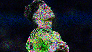
(c)

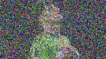
(d)

Figure 1: Illustration of an image being affected by different distortion rate via the communication channel. a) the original image, b) image affected by Gaussian noise with variance of 25, c) image affected by spackle noise with variance of 1, d) image affected by Gaussian noise with variance of 250.

Similar to human’s cognitive, AI models can experience degradation when exposed to training images with noise levels exceeding a specific threshold. Therefore, by setting a specific threshold for image distortion rates (effectively limiting the distortion introduced during communication), we can guarantee that our AI model at the receiver functions and learns effectively. This approach allows us to assess the performance of a goal-oriented semantic communication system while disregarding the accuracy achieved through the learning process as a factor influencing the evaluation of the communication system’s efficiency. More specifically, our proposed approach will contribute solutions to each of these challenges. For instance:

• In response to the first challenge, our developed approach for semantic distortion provides a unifying solution that allows all other semantic features to be transformed into distortion rates. This achievement enables the consideration of semantic optimization across various AI tasks within a unified semantic network.

• In response to the second challenge, we work to mitigate the semantic distortion rate, thus approximating the divergence in importance among AI tasks resulting from data distortion rates induced by wireless channels. This allows us to examine the relationship between prediction distortion and data distortion. Moreover, by adopting the distortion rate perspective throughout the process, we can consistently evaluate the entire network system.

Our main contributions are summarized as follows:

• We undertake a comprehensive analysis of the SemCom process within the framework of information theory, particularly focusing on distortion rates. Consequently, the entire SemCom process, encompassing the transmission model, semantic compression model, and AI task model, can be consistently and comprehensively evaluated through a unified formulation.

• To minimize semantic transmission time, we develop an approach that adaptively determines optimal semantic compression ratios, wireless resource allocation, and beyond-Shannon data rates to meet the lower-bound requirements for task performance decisions. By framing the problem in terms of distortion rates, we make it amenable to online learning.

• Addressing the challenges posed by the non-convex and intricate nature of the problem, we employ a reinforcement learning approach. This enables the agent to automatically search for the global optimal solution to our proposed problem.

• We conduct a series of rigorous experiments to validate the efficacy of our proposed algorithm. It shows significant improvements in transmission rates compared to conventional communication processes while concurrently maintaining the desired performance levels of AI tasks.

This paper is structured as follows. Section II-A describes the system model and preliminaries. Section III explains the problem formulation. Section IV presents the deep reinforcement learning approach to solve the problem. Sections A and V reports the experimental settings and results, respectively. Section VI concludes the paper.

II System Model and Fundamentals

Consider a wireless system consisting of $U$ users and one Base Station (BS) as illustrated in Figure 2. Each user transmits semantic information to the BS. To be more specific, the transmitter comprises a semantic encoder responsible for extracting semantic features from the source data. It also includes a semantic compression model tasked with compressing the semantics to reduce the transmitted data volume. Additionally, a channel encoder generates symbols to facilitate the transmission subsequently. The BS acts as a receiver and is equipped with a channel decoder for symbol detection. Furthermore, it features a semantic decoder that produces semantic concepts relevant to the tasks. An AI model is integrated into the BS to perform intelligent computing according to the received semantics, and the BS returns the task results back to users. In our research, we categorize AI tasks into two operations: AI training process and AI execution.

II-A System Model

To execute the transmission of source information on each user $u$, the semantic transmitter first extracts its meaning. This process involves sequentially encoding the original data through semantic and channel encoders. Hence, the encoded symbols, $\mathbf{x}$, can be expressed as

$$\mathbf{x}=f_{\alpha}\left(f_{\beta}(\mathbf{s})\right),$$ (1)

where $\mathbf{x}\in\mathbb{C}^{M\times 1}$, $f_{\beta}(\cdot)$ represents the deep semantic encoder network with the parameter set $\mathbf{\beta}$ and $f_{\alpha}(\cdot)$ represents the channel encoder with the parameter set $\mathbf{\alpha}$. If $\mathbf{x}$ is transmitted, the signal is affected by the wireless channel, denoted as $P(\mathbf{\hat{x}}|\mathbf{x})$ (i.e., the distributional probability of received signal $\mathbf{\hat{x}}$ given the transmitted signal $\mathbf{x}$). The transmission process from the transmitter to the receiver can be modeled as

$$\mathbf{y}=\mathbf{h_{u}}\cdot\mathbf{x}+\mathbf{n_{u}}$$ (2)

where $\mathbf{y}\in\mathbb{C}^{M\times 1}$, $\mathbf{h_{u}}$ represents the Rayleigh fading channel, and $\mathbf{n_{u}}\sim\mathcal{C}\mathcal{N}(0,\sigma^{2}_{\textrm{model},u})$ denotes independent and identically distributed (i.i.d) Gaussian noise vector with variance $\sigma^{2}_{\textrm{model},u}$ for each channel between user $u$ and the BS.

At the receiver, the received data is firstly decoded by the channel decoder $g_{\alpha}(\cdot)$ and then by the semantic decoder $g_{\beta}(\cdot)$. In the semantic decoder, the compressed data is decoded using the following equation:

$$\mathbf{\hat{s}}=g_{\beta}(g_{\alpha}(\mathbf{y})).$$ (3)

Here, $g_{\alpha}(\cdot)$ and $g_{\beta}(\cdot)$ represent the channel decoder and semantic decoder, respectively. After the data is decoded at the BS, it is employed for either AI training (during the AI training process) or AI inference (during the operational process).

II-B Communication Model

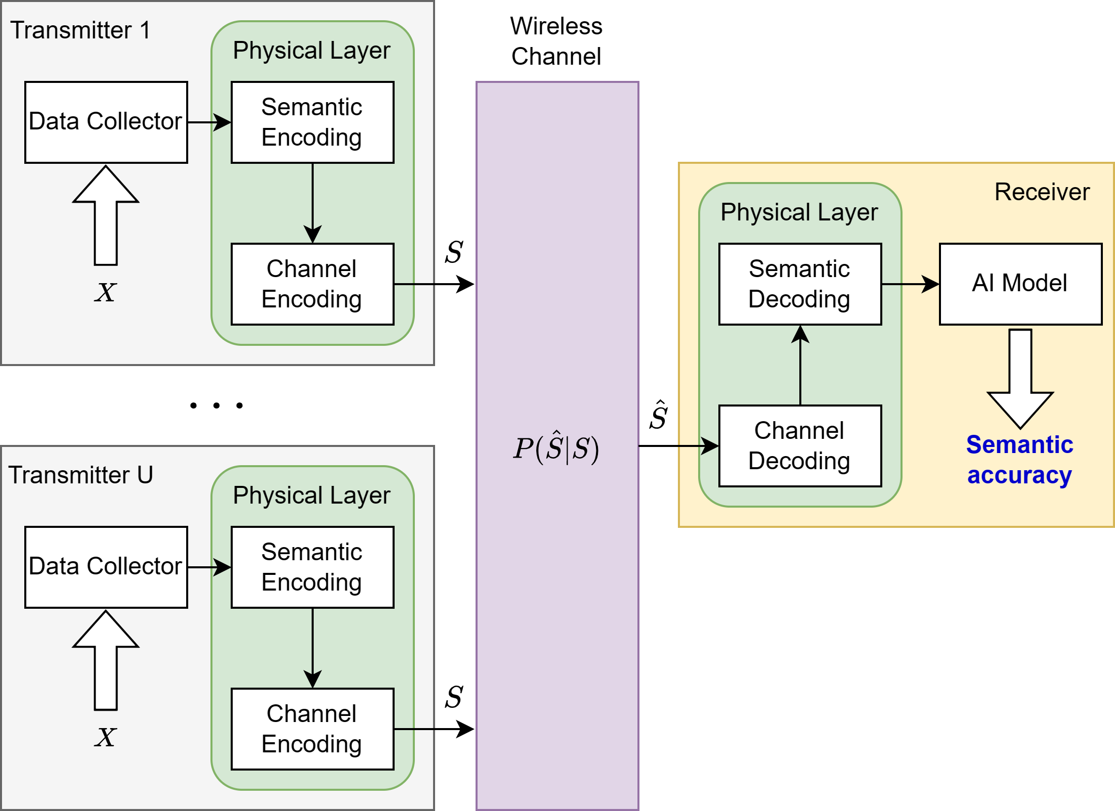
Figure 2: System Model of the considered Semantic Communication.

II-B1 Wireless Transmission

In our design, we focus on dealing with the goal-oriented system for SemCom. To characterize the performance of this goal-oriented system, we consider the distortion rate as a semantic feature. Thus, without loss of generality, we can consider the conventional Shannon Communication for our data transmission process. Therefore, the data rate for user $u$ is denoted as $R$, and it is expressed by the following equation:

$$R(B_{u},P_{u}) =B_{u}\log_{2}\left(1+\frac{h_{u}P_{u}}{I_{n}+B_{u}N_{0}}\right),$$ (4)

where $B_{u}$ denotes the bandwidth allocated to user $u$, $P_{u}$ is the transmit power of user $u$, and $N_{0}$ is the noise power spectral density. Additionally, $h_{u}=r_{u}d_{u}^{-2}$ represents the channel gain between user $u$ and the BS, where $d_{u}$ is the distance between user $u$ and the BS, and $r_{u}$ is the Rayleigh fading parameter.

II-B2 Compression Model

As discussed in Section II-A, we consider a semantic encoder/decoder model, aiming to extract the knowledge and compress the data into compact and structured representations. To assess the performance of the semantic encoder/decoder, we use two main features for each user $u$: the compression ratio and the semantic reconstruction rate, denoted as $o_{u}$ and $\sigma_{\textrm{sem},u}$, respectively. Regarding the semantic compression ratio, we employ the deep neural network for data compression [17], where the compression ratio $o_{u}$ can be characterized as the ratio between the dimensionality of the latent representation and that of the original data:

$$o_{u}=\frac{\textrm{dim}(z_{u})}{\textrm{dim}(x_{u})},$$ (5)

where $z_{u}$ denotes the latent representations induced by the semantic compressor of user $u$, and $x_{u}$ denotes the original data inputs into the semantic compressor of user $u$, respectively. To approximate the semantic reconstruction rate, we leverage the mean square error (MSE) metric between reconstructed data $\hat{x}_{u}$ and original data $x_{u}$ as $\textrm{MSE}(x_{u},\hat{x}_{u})=\frac{1}{N}\sum^{N}_{i=1}(x_{i,u}-\hat{x}_{i,u})^{2}$. As discussed in [17], the deep neural network can be considered as restricted Boltzmann machine (RBM), and thus, the noise can be modeled by a Gaussian distribution $\mathcal{N}(0,\sigma^{2}_{\textrm{sem}})$ with mean $0$ and variance $\sigma^{2}_{\textrm{sem}}$. This leads to the following relationship:

$$\sigma_{\textrm{sem},u}=\sigma_{\textrm{sem}}(o_{u}) =\sqrt{\frac{1}{N}\sum^{N}_{i=1}(x_{i,u}-\hat{x}_{i,u})^{2}}$$

$$=\sqrt{\textrm{MSE}(x_{u},\hat{x}_{u})}.$$ (6)

Here, the variance $\sigma^{2}_{\textrm{sem},u}$ can be considered as a non-linear function affected by the compression ratio $o_{u}$ (i.e., $\sigma^{2}_{\textrm{sem},u}=f(o_{u})$). Traditionally, the relationship between $\sigma^{2}_{\textrm{sem},u}$ and $o_{u}$ is regarded as impartial, implying that the distortion rate varies depending on the specific compression technique employed. Consequently, establishing a universal approximation for $f(o_{u})$ is challenging. Nevertheless, it should be noted that the compression technique is chosen before setting up the semantic communication system. As a result, we can select the compression ratio from a predefined table (an example of such a table can be found in Section A-D).

II-B3 Information Transfer

We assume that each communication round, users need to transmit an amount of $Z_{u}$ gigabits (Gb) from their respective distributed regions to the BS to execute the AI process. We denote $o_{u}$ as a semantic compression ratio on user $u$. Thus, user $u$ transmits an amount of $o_{u}Z_{u}$ Gb in each communication round. As a result, the semantic transmission time for user $u$ can be calculated as follows:

$$T_{\textrm{sem}}^{u}(B_{u},P_{u},o_{u},\beta_{u})=\frac{\beta_{u}o_{u}Z_{u}}{R(B_{u},P_{u})},$$ (7)

where the existence of $\beta_{u}$ indicates that when the user $u$ is not assigned to send the data to the server (i.e., $\beta_{u}=0$), the transmission time required for user $u$ is zero. The energy consumption at each user $u$ for sending data is given by:

$$E_{\textrm{sem}}^{u}(B_{u},P_{u},o_{u},\beta_{u})=\frac{P_{u}\beta_{u}o_{u}Z_{u}}{R(B_{u},P_{u})},$$ (8)

For this reason, the total communication energy of the system can be expressed as:

$$E_{\textrm{tot}}=\sum^{U}_{u=1}E_{\textrm{sem}}^{u}(B_{u},P_{u},o_{u},\beta_{u})=\frac{P_{u}\beta_{u}o_{u}Z_{u}}{R(B_{u},P_{u})},$$ (9)

II-C Goal-Oriented Deep Learning Model

Apart from other goal-oriented SemCom researches, we consider a general AI task capable of representing various AI tasks (e.g., natural language processing (NLP), image processing (IP), time series prediction (TSP)). The objective of the AI task-based SemCom system is to retrieve the output $\mathbf{t}$ with respect to the task’s requirement. For instance, the output could encompass an image in the case of image retrieval, a label in the context of image classification, or text for speech recognition, depending on the nature of the task.

• AI Inference: according to [18], the output probability $p(\mathbf{t})$ can be expressed as:

  $$p(\mathbf{t})=p(\mathbf{t}|\mathbf{\hat{s}})p(\mathbf{\hat{s}}),$$ (10)

  where $p(\mathbf{t}|\mathbf{\hat{s}})$ is the posterior probability.

• AI Training: Consider the AI training task at the receiver, the AI model employs a gradient descent algorithm according to a specific loss function, denoted as $F(w;\cdot)$, which can be utilized with any metric (e.g., Mean Square Error: $F(w;\mathbf{x})=\|\mathbf{t}-\mathbf{\hat{s}}\|^{2}$, Cross Entropy: $F(w;\mathbf{\hat{s}})=-f\sum_{\mathbf{\hat{s}}\in S}p(\mathbf{t})\log(\mathbf{\hat{s}})$).

II-C1 Semantic Distortion

To analyze the entire SemCom system, we treat it as a sequential stochastic process. In this regard, we introduce the following lemma concerning the sequential distortion rate:

Lemma 1.

The total distortion rate of the consequential Gaussian model for each user $u$ is given by:

$$\sigma_{\textrm{tot},u}^{2}=\sum^{L}_{l=1}\sigma^{2}_{l,u},$$ (11)

where $l$ denotes the index of the distortion generated components in the semantic communication system.

Proof: The proof is demonstrated in Appendix B.

Lemma 1 establishes a connection between a system comprising an arbitrary number of Gaussian models and the overall rate of distortion it incurs. As a result, we can formulate a joint distortion rate function that accommodates various network configurations. In our research, we introduce a straightforward system model for the Semantic Communication system, which is elaborated upon in Section II-A. Thus, we have the following Theorem:

Theorem 1.

The total distortion rate of the SemCom Process on user $u$ is approximated by:

$$\sigma^{2}_{\text{tot},u}=\sigma^{2}_{\text{sem},u}+\sigma^{2}_{\text{model},u}+\sigma^{2}_{\text{data},u}$$ (12)

Proof.

The proof is demonstrated in Appendix D. ∎

Theorem 1 shows us that the entire semantic system is affected by the three components: 1) semantic distortion rate (i.e., the noise $\sigma_{\textrm{sem},u}$ induced by the information loss in lossy compression on each user $u$, the ), 2) channel distortion rate (i.e., the noise $\sigma_{\textrm{model},u}$ induced by the channel model), and 3) data distortion rate (i.e., the noise $\sigma_{\textrm{data},u}$ induced by the data sampling process).

II-C2 Deep Learning Model Variance

To analyze the distortion impact on model predicting variance, we make the following two assumptions on the empirical distance function:

Assumption 1 ($L$-smooth).

Function $F$ is $L$-Lipschitz smooth, i.e., $\nabla^{2}F\leq L\mathbf{I}$.

Assumption 2 ($\mu$-strongly convex).

Function $F$ is $\mu$-strongly convex, i.e., $\nabla^{2}F\geq\mu\mathbf{I}$.

Here, we denote $\mathbf{I}$ as an identical matrix. We follow the following assumption to analyze the model variance:

Assumption 3.

Given the global dataset $\mathcal{D}=\{(x_{i},y_{i})|y_{i}\in\{1,2,\dots,C\}\}$, there always exists canonical data point $\widetilde{x}=\{\widetilde{x}^{c}|c\in\{1,2,\dots,C\}\}$ respect to data region $c$ which satisfy $\widetilde{x}^{c}=\lim_{j\rightarrow\infty}\sum^{j}_{i=1}(x_{i}|y_{i}=c)$.

Training phase: We consider a training phase, where the task oriented AI model leveraged the data collected from all users $u\in U$ for the training process. Therefore, the training data batch is sampled from a data pool, which is the joint distribution of all distributed domain. To characterize the total distortion of the system with $U$ users, we have to consider the following lemma:

Lemma 2.

Giving each user $u\in U$ sampled data from different domains. We have the learning data at the server sampled from a data pool, which can be considered as the joint distribution among all devices’ data distribution, thus we have the servers’ data variance can be considered as:

$$\sigma^{2}_{\textrm{tot}} =\frac{1}{D}\sum^{U}_{u=1}D_{u}\sigma^{2}_{\textrm{tot},u},$$ (13)

where $D_{u},D$ are the number of data stored on user $u$ and of all user ($D=\sum^{U}_{u=1}D_{u}$), respectively.

Applying the assumptions 1, 2, and 3, and lemma 2, we have the following theorem on training divergence when using noisy data induced by wireless channel:

Theorem 2.

Given $\sigma_{\textrm{tot}}^{2}$ is the average distortion on data compared to the global ideal data $\widetilde{x}$ in the dataset $\mathcal{D}$, the learning error bounds of the distorted data on the hypothesis $h_{\theta}$ after $N$ training rounds is demonstrated as follows:

$$F(w^{n};\hat{x})-F(w^{n};x)\leq N\left(\eta^{2}\frac{L}{2}-\eta\right)(L\sigma_{\textrm{tot}})^{2},$$ (14)

where $\sigma_{\textrm{tot}}$ represents the expected total distortion of the system including $U$ users.

Proof: The proof is demonstrate in Appendix E.

The Theorem 2 assists us in estimating the degradation in AI training performance caused by semantic noise present in the data. By utilizing data distortion as a proxy for approximating AI performance, rather than directly relying on AI metrics (i.e., accuracy or semantic similarity), we gain the ability to anticipate AI performance prior to the completion of data transmission. This approach, similar to the work presented in [12, 13, 11], empowers us to proactively consider goal-oriented AI performance. Consequently, this paves the way for optimizing neural networks in the context of Goal-oriented Semantic Communication.

Inference phase: In the inference phase, the AI task performance needs to be approximated via one data point. Therefore, we can not use statistical measurement to consider the generalization gap as in the training phase. To consider the inference capacity of the AI model under a noisy channel, we first adopt the following lemma:

Lemma 3.

Given the data $x$ and the noisy data $\hat{x}$ induced by the semantic noisy channel, we have the following total variation between the distribution of two data as follows:

$$\textrm{TV}(x,\hat{x})\leq\frac{1}{\sqrt{2\pi}\sigma}\exp{-\left(\frac{W}{2\sigma}\right)^{2}},$$ (15)

where $W$ is the decision boundary of data changes that can preserve the goal-oriented AI task, $sigma$ denotes the distortion rate between the original data and the noisy data. Thus, we can measure the distribution shift between two data via the amount of data components’ distortion that pass the decision boundary.

To be more intuitive, for a basic task like spotting if there’s a person in a Figure 1d, the AI can handle a lot of changes in the image without a problem. But for a tougher task like figuring out who that person is, the AI needs data with more clear details. If there are big changes, like in Figure 1d, it might not recognize the person correctly. This shows that the complexity of the task affects how much change the AI can handle. Therefore, we have the following theorem:

Theorem 3.

The inference gap of the semantic AI model under the noisy channel can be represented as:

$$\mathbb{E}\left[p(\mathbf{\hat{t}})-p(\mathbf{t})\right]\leq\frac{1}{\sqrt{2\pi}\sigma}p(\mathbf{t}|\mathbf{s})\exp{-\left(\frac{W}{2\sigma}\right)^{2}}$$ (16)

Proof: The proof is demonstrate in Appendix I.

Through the utilization of Theorem 3, we gain the capability to predict the decline in AI model performance resulting from input data distortion in comparison to the pristine original data. The salient aspect of Theorem 3 lies in its ability to gauge the deterioration of the AI model on a per-data-point basis. Consequently, during the process of optimizing the network while the AI task is in progress, there is no longer a necessity to draw a substantial amount of data samples in order to approximate the shift in data distribution, as was required in the case of Theorem 2.

III Problem Formulation

To jointly design a data distortion-driven task-oriented SemCom system, we formulate two optimization problems, which consider the optimization process of semantic system under two distinguish AI phases: AI training and AI inference.

III-A Optimization Problem for Semantic AI Training Process

In the AI training phase, we consider the learning performance of the AI model from scratch until divergence. Specifically, we optimize the total communication energy, while maintaining the AI learning performance. To this end, we aim to have the distortion rate always have an upper bound to ensure that the DL tasks do not diverge more than an arbitrary threshold. The optimization problem is given as

$$\min_{\mathbf{B},\mathbf{P},\mathbf{o},\mathbf{\beta}} \leavevmode\nobreak\ E_{\textrm{tot}}(\mathbf{B},\mathbf{P},\mathbf{o},\mathbf{\beta})=\sum^{U}_{u}E_{\textrm{sem}}^{u}(B_{u},P_{u},o_{u},\beta_{u}),$$ (17a)

s.t. $$B_{u}\geq 0,\forall u\in U,$$ (17b)

$$\sum^{U}_{u=1}\beta_{u}B_{u}\leq B_{\textrm{max}},\forall u\in U,$$ (17c)

$$0\leq P_{u}\leq P_{\textrm{max}},\forall u\in U,$$ (17d)

$$0<o_{u}<1,$$ (17e)

$$\sigma_{\textrm{sem},u}=f(o_{u}),$$ (17f)

$$\beta_{u}\in\{0,1\},$$ (17g)

$$\left(\eta^{2}\frac{L}{2}-\eta\right)(L\sigma_{\textrm{tot}})^{2}<\varepsilon_{\textrm{learn-target}},$$ (17h)

where $\sigma_{u}$ is the variance of the model’s output prediction corresponding to the distorted data at the user’s receiver over $U$ user. We denote $\mathbf{\beta}=\{\beta_{1},\beta_{2},\cdots\beta_{U}\}$ as the set of user selection, $\mathbf{P}=\{P_{1},P_{2},\cdots P_{U}\}$ as the set of user power, $\mathbf{o}=\{o_{1},o_{2},\cdots,o_{U}\}$ as the set of compression coefficients. Constraint (17c) indicates that the sum bandwidth of selected users cannot exceed a given threshold, which refers to the system bandwidth. Constraint (17b) and (17d) are the minimum bandwidth and the minimum transmit power constraints, respectively. Constraint (17e) is the compression ratio constraint bounded by 1 (i.e., the data without compression). Constraint (17f) implies the semantic distortion rate follows the relationship between the distortion rate and compression ratio of specific compression algorithm. The semantic relationship can be used by approximation function or mapping table (i.e., we deploy and evaluate the semantic compression algorithm prior to the DRGO deployment). Constraint (17h) is the distortion rate resilience constraint. Specifically, we want to ensure that the total distortion rate is lower than the certain threshold (i.e., the threshold that the task predictor can achieve a minimal accuracy $\varepsilon_{\textrm{learn-target}}$). The main notations of this paper are summarized in Table. I.

III-B Optimization Problem for Semantic AI Executing Process

To jointly design a data distortion-driven task-oriented SemCom system, we formulate a problem to optimize the total communication energy, while factoring the wireless network parameters. Particularly, we have a joint distortion constraints, where the distortion rate always have an upper bound to ensure that the DL tasks do not diverge more than an arbitrary threshold. The optimization problem is given by:

$$\min_{\mathbf{B},\mathbf{P},\mathbf{o},\mathbf{\beta}} \leavevmode\nobreak\ E_{\textrm{tot}}(\mathbf{B},\mathbf{P},\mathbf{o},\mathbf{\beta})=\sum^{U}_{u}E_{\textrm{sem}}^{u}(B_{u},P_{u},o_{u},\beta_{u}),$$ (18a)

s.t. $$B_{u}\geq 0,\forall u\in U,$$ (18b)

$$\sum^{U}_{u=1}\beta_{u}B_{u}\leq B_{\textrm{max}},\forall u\in U,$$ (18c)

$$0\leq P_{u}\leq P_{\textrm{max}},\forall u\in U,$$ (18d)

$$0<o_{u}\leq 1,$$ (18e)

$$\sigma_{\textrm{sem},u}=f(o_{u}),$$ (18f)

$$\beta_{u}\in\{0,1\},$$ (18g)

$$\frac{1}{\sqrt{2\pi}\sigma}p(\mathbf{t}|\mathbf{s})\exp{-\left(\frac{W}{2\sigma_{\textrm{tot}}}\right)^{2}}<\varepsilon_{\textrm{inf-target}},$$ (18h)

where $\sigma_{u}$ is the variance of the model’s output prediction corresponding to the distorted data at the user’s receiver over $U$ user. We denote $\mathbf{\beta}=\{\beta_{1},\beta_{2},\cdots\beta_{U}\}$ as the set of user selection, $\mathbf{P}=\{P_{1},P_{2},\cdots P_{U}\}$ as the set of user power, $\mathbf{o}=\{o_{1},o_{2},\cdots,o_{U}\}$ as the set of compression coefficients. Constraint (18c) indicates that the sum bandwidth of selected users cannot exceed a given threshold, which refers to the system bandwidth. Constraint (18b) and (18d) are the minimum bandwidth and the minimum transmit power constraints, respectively. Constraint (18e) is the compression ratio constraint bounded by 1 (i.e., the data without compression). Constraint (18f) implies the semantic distortion rate follows the relationship between the distortion rate and compression ratio of specific compression algorithm. The semantic relationship can be used by approximation function or mapping table (i.e., we deploy and evaluate the semantic compression algorithm prior to the DRGO deployment). Constraint (18h) is the distortion rate resilience constraint. Specifically, we want to ensure that the total distortion rate is lower than the certain threshold (i.e., the threshold that the task predictor can achieve a minimal accuracy $\varepsilon_{\textrm{inf-target}}$).

IV Deep Reinforcement Learning Approach for DRGO

In this section, we briefly introduce the structures and process of our DDPG-based algorithm. In order to utilize DRL to solve the minimization problem, we must redesign the optimization problem so that the algorithm process should be properly considered following the DRL operating rule.

IV-A Closed-form expression for Optimization Problem

To make the optimization problems in (17a), (18a) feasible for DRL, we first need to find the closed form of the optimization problems. To this end, we first classify the constraints in the optimization problem into two categories, subbed Explicit constraints and Ambiguous constraints.

IV-A1 Explicit Constraints

The Explicit constraints refers to as the constraints that are easily to be configurable. These constraints mostly focus on the limits of system variables (e.g., power, bandwidth). Taking advantage of the outputs of a deep model can lead to substantial improvements in these components without incurring significant computational costs. More specifically, we alternatively describe the constraint by exploiting the basic activation function. (i) To restrict the variables to the specific range (e.g., $0\leq P\leq P_{\textrm{max}}$), we first use the sigmoid function. Afterwards, the data is normalized to the appropriate range using the normalization function. (ii) In order to impose a limit on the value, while ensuring that the variables are always constrained to sum to a value lower than a predetermined threshold (e.g., $0\leq\sum_{u}Bu\leq B$), we make use of the softmax function. Subsequently, we can use the normalization process (which is similar to (i)).

Implementing this approach can simplify the loss function and improve the performance of the DRL algorithm. Instead of incorporating constraints directly into the reward function, the constraints are hard-fixed, resulting in variables being automatically limited to the required bounds. This simplifies the loss function, avoiding the complexities introduced by constraints, and avoiding the stronger non-convexity of the loss function. Moreover, this approach enhances the model’s adaptability, allowing it to quickly learn and adapt to new constraints. By reducing the computational complexity and increasing the adaptability of the system, we can optimize performance without compromising the quality of results. Furthermore, this approach can greatly enhance the performance of the DRL algorithm by allowing the model to learn and adapt to new constraints quickly.

IV-A2 Ambiguous Constraints

Contrary to explicit constraints, the ambiguous constraints are more difficult to configure and cannot simply be done by normalizing the model’s output. We use the Lagrange approach [19] to resolve this issue.

IV-B Designing Observation for DRGO

IV-B1 State Space

Let $h^{t}_{u}$ denote the channel gain with the base station and the user i at the time step $t$. Then, the state space of the system, denoted by $S$, is defined as:

$$\mathbf{s}^{t}=\{h^{t}_{1},\cdots h^{t}_{U}\}.$$ (19)

As a consequence, the state space $\mathbf{S}$ can be defined as $\mathbf{S}=\{\mathbf{s}^{1},\cdots,\mathbf{s}^{T}\}$, where $T$ is the total number of time steps used for the RL training phase.

IV-B2 Action Space

Denoted $\mathbf{A}$ as action space of the system. Given a certain state s, a control action is performed to determine $\mathbf{\beta}=\{\beta_{1},\beta_{2},\cdots\beta_{U}\}$ as the set of user selection, $\mathbf{P}=\{P_{1},P_{2},\cdots P_{U}\}$ as the set of user power and $\mathbf{o}=\{o_{1},o_{2},\cdots,o_{U}\}$ as the set of compression coefficients. Thus, $\mathbf{A}$ can be defined as: $\mathbf{A}=\{\beta_{1},P_{1},o_{1},\cdots\beta_{U},P_{U},o_{U}\}$

IV-B3 Reward Space

Based on the system model we proposed above, we want to optimize the total communication energy while maintaining the AI performance according to different tasks (AI model during the task execution, and during the task training process). Due to the requirement of minimizing total consuming time over time, we use the total communication energy as the reward. To this end, we aim to have the distortion rate always have upper bound to ensure that the DL tasks do not diverge more than an arbitrary threshold, so we use that to the penalty. Therefore, the reward can be defined as $\mathcal{R}=\{r^{1},\ldots,r^{T}\}$. We define the immediate reward $r^{t}$ as:

$$r^{t}=-\sum\nolimits_{u=1}^{U}E_{\textrm{sem}}^{u}+\lambda\mathcal{P},$$ (20)

where the subscript $\lambda$ is the coefficient that controls the goal-oriented regularization. The penalty $\mathcal{P}$ is defined as the constraints on Distortion Resilience according to different agent’s settings. The core concept behind these constraints is that if a distortion resilience value surpasses a predetermined threshold, the AI model aims to minimize the deviation from that threshold. Specifically, we have the penalty function for Training Resilience task III-A as follows:

$$\mathcal{P}=\max{\left\langle\left[\left(\eta^{2}\frac{L}{2}-\eta\right)\left(L\sigma_{\mathrm{tot}}\right)^{2}-\varepsilon_{\textrm{learn-target}}\right],0\right\rangle},$$ (21)

and the penalty function for Inference Resilience task III-B).

$$\mathcal{P}=\max{\left\langle\left[\frac{1}{\sqrt{2\pi}\sigma}p(\mathbf{t}|\mathbf{s})\exp{\frac{-W^{2}}{2\sigma^{2}_{\textrm{tot}}}}-\varepsilon_{\textrm{inf-target}}\right],0\right\rangle},$$ (22)

where the $\max(\cdot)$ function imitates the resilience property, which only captures the penalty only when the distortion rate passes the upper threshold (i.e., where the AI task’s performance is preserved). As it can easily be seen from the equation (20), we only consider the Distortion Resilience as penalty as other constraints (17e), (17c), (17b), (17d), (17g) are considered by tuning the action output as mentioned in Section IV-A1.

Given the immediate reward defined as in Equation (20), we have the accumulative long-term reward for the system, which can be expressed as follows:

$$\mathcal{R}(\pi)=\sum^{I_{\textrm{glob}}}_{t}\gamma^{I_{\textrm{glob}}-t}\mathbf{r}^{t}(s^{t},\pi(s^{t})),$$ (23)

where $\mathcal{R}(\pi)$ is the accumulative long-term reward of the agent under policy $\pi(\cdot)$ and $\mathbf{r}^{t}(s^{t},\pi(s^{t}))$ at time step $t$. The subscript $\gamma$ denotes the discount factor for the reward that reflects how much the reward depends on the past performance (i.e., when $\gamma$ is near $0$, the policy evaluation ignores the historical performance, and vice versa).

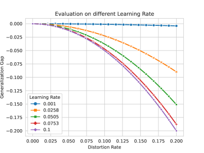
(a)

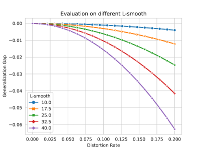
(b)

Figure 3: Illustration of the training gradient inductive bound (a) with different $L$-smooth, and (b) with different learning rate $\eta$.

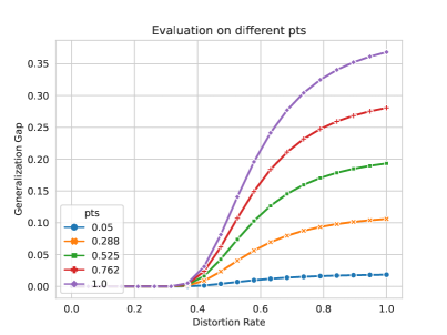
(a)

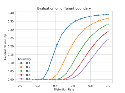
(b)

Figure 4: Illustration of the inference generalization gap (a) with different decision boundaries, and (b) with different model accuracy.

IV-C DRGO Architecture

As mentioned in IV-A1, we redesign the DRGO architecture.

IV-C1 An Overview of DDPG

DDPG (Deep Deterministic Policy Gradient) is a widely used technique in DRL. It employs four neural networks, which are described below:

• The actor network, also known as the policy network, is parameterized by $\phi_{\mu}$. It takes the state $s$ as input and produces an action denoted by $\pi(s|\phi_{\mu})$.

• The target actor network, parameterized by $\phi_{\mu_{t}}$, generates the target policy $\pi(s|\phi_{\mu_{t}})$.

• The critic network, also referred to as the $Q$ network, is parameterized by $\phi_{q}$. It takes both the state $s$ and the action $a$ as inputs and outputs the corresponding state-value function $Q(s,a|\phi_{q})$.

• The target critic network, parameterized by $\phi_{q_{t}}$, produces the target state-value function $Q(s,a|\phi_{q_{t}})$.

IV-C2 Training of the Critic Network

The batch of observations is sampled from the experience replay buffer $D$. The target value $Q$ of the $k^{\textrm{th}}$ observation $(s_{k},a_{k},r_{k},s_{k+1})$ is represented by $y_{k}$:

$$y_{k}=r_{k}+Q(s_{k+1},a_{k+1}|\phi_{q}),$$ (24)

where $a_{k+1}$ is the action sampled by the DRGO network at step $k+1$ via the policy $a_{k+1}\sim\pi(s_{k+1}|\phi_{\mu})$ under the influence of $s_{k+1}$ through the target actor network. The subscript $Q(s_{k+1},a_{k+1}|\phi_{q})$ defines the output of the target critic network. We obtain the critic network’s optimal parameters $\phi_{q}^{*}$ by minimizing the MSE between estimated $Q$ value of the critic network $Q(s_{k},a_{k}|\phi_{q})$ and the $Q$ target $y_{k}$:

$$\phi_{q}^{*}= \arg\min_{\phi_{q}}\leavevmode\nobreak\ \mathcal{L}(\phi_{q}),$$ (25a)

s.t. $$\mathcal{L}\left(\phi_{q}\right)=\frac{1}{N_{B}}\sum_{k=1}^{N_{B}}\left(y_{k}-Q\left(s_{k},a_{k}|\phi_{q}\right)\right)^{2}.$$

IV-C3 Training the Actor Network

In order to improve the policy obtained from the proposed algorithm, the parameters of the agent network must be updated so that the action output from the agent network is in the direction of increasing the Q value, which is the output from the critic network. By using gradient descent, the optimal parameters of the actor network $\phi_{\mu}^{*}$ can be updated via the following optimization function:

$$\phi_{\mu}^{*}= \arg\max_{\phi_{\mu}}\leavevmode\nobreak\ \mathcal{L}(\phi_{\mu}),$$ (26a)

s.t. $$\mathcal{L}\left(\phi_{\mu}\right)=\frac{1}{N_{B}}\sum_{k=1}^{N_{B}}Q\left(s_{k},\pi(s_{k}|\phi_{\mu})|\phi_{q}\right).$$

IV-C4 Slow Update of Critic and Actor Network

Continuous updates of the actor and actor network models are necessary in DRL to enhance system performance. However, excessively frequent updates can result in unstable and erratic fluctuations of the model’s parameter values. This instability can lead to overfitting, restricting the model’s ability to generalize to novel scenarios beyond the training dataset. Furthermore, frequent updates can disrupt the delicate balance between exploration and exploitation within the system. When the actor is updated too frequently, it may fail to explore sufficient new actions to identify the optimal values for novel states. Similarly, frequent updates of the actor can yield unstable and unreliable action values, impeding the efficiency of the learning process.

Table I: Table of abbreviations and notations.

Notation	Description
$U$	Number of users
$B_{u}$	Bandwidth of user $u$
$o_{u}$	Semantic compression ratio of user $u$
$D$	Number of data stored on server’s data pool
$D_{u}$	Number of data of user $u$ stored on server
$B_{\textrm{min}}$	Minimum bandwidth allocated to users
$B_{\textrm{max}}$	Maximum total bandwidth
$P_{\textrm{min}}$	Minimum transmit power allocated to users
$P_{\textrm{max}}$	Maximum total transmit power
$F(w;\cdot)$	Goal-oriented AI loss function
$\mathbf{\beta}$	User selection vector
$\mathbf{x_{u}}$	Source data on user $u$
$\mathbf{\hat{x}_{u}}$	Reconstructed data on user $u$
$\mathbf{s}$	Encoded data
$\mathbf{\hat{s}}$	Received encoded data

To address the aforementioned issues, the sub networks (i.e., target actor and critic) are employed in order to update the actor and actor networks at a slower pace. This approach ensures stability and maintains a balance between exploration and exploitation throughout the learning process. The actor is accompanied by a slower updated target actor. The target actor is a replica of the actor, but its parameters $\phi_{q_{t}}$ are updated gradually using a weighted average of the actor’s parameters $\phi_{q}$. Specifically, parameters set of the target actor is computed by taking a fraction (commonly denoted as $\beta$, with values like $0.001$ or $0.005$) of its current value and adding $(1-\beta)$ times the new value from the main actor network. The parameters of the target critic network are updated according to the following function:

$$\phi_{q_{t}}=\beta\phi_{q}+(1-\beta)\phi_{q_{t}},\quad 0<\beta<1.$$ (27)

Similar to the slow update for target critic, we implement slow updates in the target actor. This technique helps minimize anomalous updates, prevents overfitting, and ultimately improves the overall learning process of the system. The parameters of the target actor are updated as follows:

$$\phi_{\mu_{t}}=\beta\phi_{\mu}+(1-\beta)\phi_{\mu_{t}},\quad 0<\beta<1$$ (28)

IV-C5 OU Noise

From the user’s perspective, the actor network is of paramount importance as it provides the desired solution. To encourage exploration of the environment, the output of the actor network is subject to the introduction of noise. The DDPG algorithm employs OU Noise for this purpose due to its two key characteristics: (1) it enables intensive exploration during the initial phase of reinforcement learning training, and (2) gradually transitions towards exploitation (i.e., reducing the noise) in the later stages of training.

IV-C6 Experienced Replay Buffer

In order for the DRL agent based on the DDPG algorithm to learn from the interaction with the environment, an experience replay $D$ is constructed. At time $t$, the DRL agent takes action $a_{t}$ under the influence of $s_{t}$, then receives a reward $r_{t}$ and is moved to the next state. Therefore, the transition tuple ($s_{t}$, $a_{t}$, $r_{t}$, $s_{t+1}$) is saved to experience replay $D$.

V Experimental Evaluations

We assess DRGO’s performance in two different schemes: AI Inference and AI Training schemes. Our experimental evaluations follow the settings explained in detail in Appendix A. Our official implementation is available on Github .

V-A DRL Training

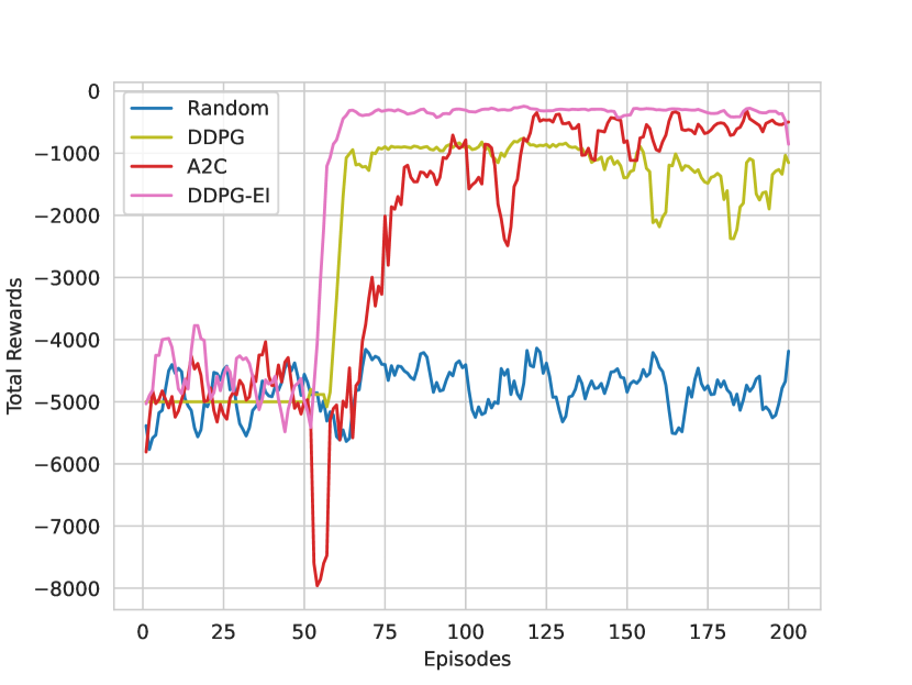
Figure 5: DRL Performance on Training Optimization Problem.

We perform an experimental evaluation on the DDPG-EI algorithm that we devised. To assess the algorithm’s quality, we compare it against various baselines, including Random Action (where actions are selected randomly). Comparing with random action serves to determine if the model enhances system quality beyond the standard level achieved without optimization. Additionally, we compare against DDPG and A2C. It’s evident that our method inherits the stability of the original DDPG approach and is less affected by noise compared to A2C. Moreover, by employing fixed constraints at the action outputs, we significantly reduce the unnecessary computational complexity of the optimization problem. As a result, DDPG-EI demonstrates relatively rapid convergence compared to the other two algorithms and yields a much improved policy compared to the remaining two baseline methods. Episodes from 0 to 50 involve random actions to populate the experience replay memory, without contributing to the training process and avoiding computation costs during this phase. With fast convergence (within only 3 episodes * 200 timesteps per episode from the start of training), the system showcases the agent’s ability to rapidly learn from the environment. Consequently, the system can adapt and perform swiftly when integrated into a network.

V-B AI Inference Phase

V-B1 Distortion Resilience Boundary

Two graphs illustrate the influence of distortion rate on the generalization gap, which is the difference in AI predicting accuracy between original data and the distorted data (accumulated from various forms of distortion during data transmission).

Figure (a) presents a comparison of AI model performance across various levels, quantified by the posterior probability $p(\mathbf{t}|\mathbf{\hat{s}})$. As depicted in the graph, higher AI performance (indicated by greater values of $p(\mathbf{t}|\mathbf{\hat{s}})$) corresponds to a wider gap in generalization between predictions made using distorted data and clean data, respectively. Another influential factor on predictive performance is the decision boundary. More specifically, as the decision boundary decreases in size, the generalization gap becomes more prominent. This is because a smaller decision boundary signifies more intricate data characteristics. For instance, referring to Figure 1, when the decision boundary is elevated, alterations like changes in player’s skin color can significantly impact the accuracy of player identity recognition.

Nevertheless, it is noticeable that the generalization gap experiences substantial impact as the distortion rate surpasses a threshold of 0.2. Consequently, it is evident that the optimal outcomes for our semantic communication system are attainable when the distortion rate falls within the range of 0.2 to 0.4.

V-B2 Different level of maximum power

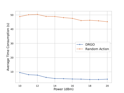
(a)

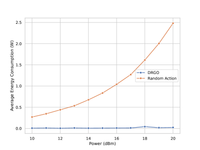
(b)

Figure 6: The average time delay and energy consumption versus the maximum transmit power of each physical device with $U$ = 10.

Figure 6b depicts the variations in total communication and computation energy as the maximum transmit power of each user varies. This figure clearly illustrates that as the maximum transmit power of the base station (BS) increases, the total energy consumption decreases. This phenomenon is a result of higher transmit power leading to reduced transmit time, thereby allowing more time for computation and ultimately resulting in lower total energy consumption. Notably, our proposed DRGO system demonstrates a remarkable improvement, achieving more than a fivefold increase in both time delay and energy efficiency. This substantial enhancement can be attributed to the DRGO system’s deliberate choice of a high compression ratio, which effectively optimizes resource allocation.

V-B3 Different number of users

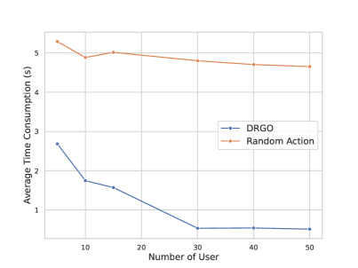
(a)

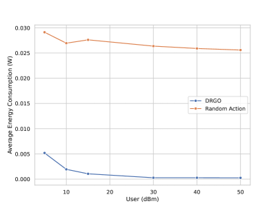
(b)

Figure 7: The average time delay and energy consumption versus the number of participating users with max power = 10 dBm.

Figures 7b and 7a illustrate how the average energy and time delay vary with changes in the maximum transmit power of each user. According to the figure, our proposed DRGO system can achieve a significant improvement in energy efficiency, exceeding a factor of $10$, while maintaining significantly lower time delays compared to random actions (specifically, reducing the time delay from a range of $2-5$ to a much lower level). This remarkable performance is primarily attributed to the utilization of compression techniques. By taking into account semantic distortion, our DRGO semantic system can proactively assess the level of distortion resilience required. Consequently, the DRGO system can opt for a very high distortion ratio, enabling compression rates exceeding 60 times that of the original data. As a result, users only need to employ very low transmission power when sending data over the wireless channel, typically less than $-3.02$ dB.

V-C AI Training Phase

V-C1 Distortion Resilience

Two graphs illustrate the influence of distortion rate on the generalization gap, which is the difference in AI training performance between the original dataset and the dataset subjected to distortion-induced noise (accumulated from various forms of distortion during data transmission).

Graph (a) compares different learning rate levels. As observed in the graph, when the learning rate is increased, the agent explores more aggressively, causing the gradient to oscillate around the minimizer instead of converging within it. This results in a significant disparity when using distorted data compared to clean data. Conversely, selecting a lower learning rate reduces the discrepancy in noise levels. However, this elongates the learning process and presents risks of gradient descent becoming trapped in sharp minimizers.

Graph (b) compares different levels of L-smoothness. L-smoothness corresponds to the dataset’s complexity (specifically, datasets with higher complexity, featuring more sharp minimizers, have larger L-smooth values). As seen, higher L-smooth values lead to greater discrepancies in error between the original and distorted data, especially with higher distortion rates. This insight indicates that optimizing DRGO also hinges on recognizing variations in dataset complexity (for instance, with complex datasets like Imagenet, employing less distortion resilience is necessary, while simpler datasets call for more resilience). Moreover, one approach to enhancing distortion resilience is to partition the AI task into simpler subtasks and carry out independent multi-task learning. This helps reduce data complexity for each specific task. Several techniques can be applied in this context, such as Disentanglement Learning, Invariant Learning, Multi-task Learning, and Meta Learning.

V-C2 Different level of maximum power

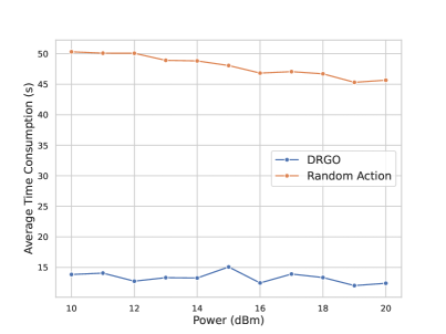
(a)

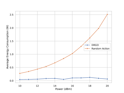
(b)

Figure 8: The average time delay and energy consumption versus the maximum transmit power of each physical device with $U$ = 10.

In Figures 8b and 8a, you can observe the fluctuations in average energy and time delay as the maximum transmit power of each user undergoes changes. The figure provides a clear depiction of the relationship between increased maximum transmit power at the base station (BS) and decreased total energy consumption. This phenomenon arises from the fact that higher transmit power leads to reduced transmission time, allowing more time for computational tasks and ultimately resulting in reduced total energy consumption. Notably, our innovative DRGO system showcases a remarkable enhancement, achieving a more than fivefold improvement in both time delay and energy efficiency. This substantial advancement can be credited to the intentional selection of a high compression ratio by the DRGO system, effectively optimizing the allocation of resources.

V-C3 Different number of users

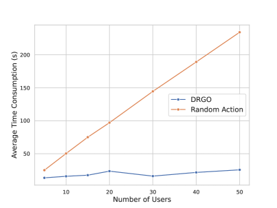
(a)

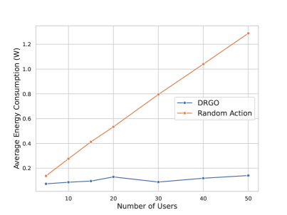
(b)

Figure 9: The average time delay and energy consumption versus the number of participating users with max power = 10 dBm.

Figures 9b and 9a provide a visual representation of how average energy consumption and time delay respond to variations in the maximum transmit power of each user. These figures underscore the impressive capabilities of our proposed DRGO system, which achieves a remarkable energy efficiency enhancement, surpassing a tenfold improvement. Additionally, it maintains significantly reduced time delays compared to random actions, notably shrinking the time delay range from 2-5 to a substantially lower level. The extraordinary performance of our system is predominantly attributed to the strategic use of compression techniques. By factoring in semantic distortion considerations, our DRGO semantic system can proactively gauge the required level of distortion resilience. Consequently, the DRGO system can select an exceptionally high distortion ratio, resulting in compression rates exceeding 60 times that of the original data. Consequently, users only need to employ very low transmission power, typically falling below -3.02 dB, when transmitting data over the wireless channel.

VI Conclusion

This paper explores efficient semantic communication by addressing wireless resource allocation and semantic information extraction while considering distortion rates. It introduces a novel approach where users transmit lossy semantic data to a base station, which then performs AI operations based on this data with predefined distortion. This research pioneers the integration of semantic distortion considerations into AI training, treating it as an optimization problem to minimize network energy consumption while accommodating generalization gaps. The paper also presents a detailed DRL solution, demonstrating the effectiveness of the proposed algorithm through numerical results.

Appendix A Experimental Settings

In this section, we study the performance of the proposed DRGO assisted Goal-oriented Semantic Communication by using computer simulation results. All statistical results are averaged over $10$ independent runs.

A-A DRL settings

In our simulations, the learning rates for actor and critic networks are $3\times 10^{-4}$ and $1\times 10^{-3}$, respectively. The reward discount parameter is $\gamma=0.99$, the network soft updating parameter is $\tau=5\times 10^{-3}$, and the batch size for the experience replay memory is $128$.

A-B System settings

For our simulations, we deploy $K=50$ users uniformly in square area of $1\textrm{km}\times 1\textrm{km}$ with the BS located at its center. The path loss model is $128.1+37.6\log_{10}d$ ($d$ is in km) and the standard deviation of shadow fading is $8$ dB. In addition, the noise power spectral density is $N_{0}=-174$ dBm/Hz.

We use CIFAR-10 [20] to evaluate the AI process. The prediction task associated with the data is the classification problem, in which we want to predict the label over $10$ other labels for the image in the dataset. The images are assumed to be sampled by distributed devices, and transfer via communication link to the BS. We choose an approximate data size of $24.528$ kbits which is related to the averaged size of CIFAR-10 images.

A-C Goal-oriented settings

To properly simulate the goal-oriented semantic communication, we must consider the AI training task. In goal-oriented AI task, the key features that capture all characteristics of training data and training AI model is $L$-smooth and $\mu$-strongly convex. To this end, we deploy a classification task on Convolutional Neural Network (CNN) on CIFAR-10 dataset [20]. We sample data and feed through the AI model to consider the Hessian of the loss function. We follow the theory [21, 22, 23] that at the initial phase of the AI training, the minimizer tends to be sharpest. Therefore, by consider the Hesisan of the loss function of the untrained AI model with specific dataset, we can have the minizer with highest $2$nd derivative value. Which is approximately close to the $L$-smooth and $\mu$ strongly convex value. Our theoretical implementation for goal oriented $L$-smooth and $\mu$ strongly convex estimation can be found via experimental evaluation code. According to our evaluation, we found that the $L$ and $\mu$ value on MNIST and CIFAR-10 dataset is higher than $10$ and $30$, respectively. Therefore, we choose the $L$ and $\mu$ for our experimental evaluation with set of values: $\{10,17,25,32.5,40\}$.

A-D Semantic Compression settings

To make the appropriate estimation for semantic compression - ratio to distortion rate, we use a simple convolutional autoencoder on CIFAR-10 dataset [20] to simulate the performance of semantic communication. To be more specific, we train the autoencoder to reconstruct the original data via the MSE function. The embedding vectors with smallest dimensionality represents the compressed representation and the compression ratio is considered via the Equation (5). Our theoretical implementation for semantic compression - ratio to distortion rate can be found via experimental evaluation code. The mapping of ratio to distortion rate is demonstrated as in table II.

Table II: Experimental Results of semantic compressors with different compression ratio.

Comp.	Data	Loss	Comp.	Data	Loss
Ratio	Dimension		Ratio	Dimension
192	16	0.799	24	128	0.193
96	32	0.539	16	192	0.131
48	64	0.337	12	256	0.098
32	96	0.249	10	312	0.079
9	341	0.069	8	384	0.060
6	576	0.034	4	768	0.020
3	1152	0.017	2	1536	0.015

Appendix B Proof on Lemma 1

Before proving the Lemma 1, we first adopt the following Lemma:

Lemma 4.

Consider the convolution of two consecutive system which follows Gaussian process (i.e., $f_{1}(x)=\mathcal{N}(0,\sigma^{2}_{1})$ and $f_{2}(x)=\mathcal{N}(0,\sigma^{2}_{2})$). The resulting function follows Gaussian process and have the resulting variance as $\sigma^{2}_{\textrm{tot}}=\sigma^{2}_{1}+\sigma^{2}_{2}$. For instance:

$$f_{\textrm{tot}}(x)=f_{1}(z)\otimes f_{2}(z)=\frac{1}{\sqrt{2\pi}\sigma_{\textrm{tot}}}\exp\left[-\frac{z^{2}}{2\sigma_{\textrm{tot}}^{2}}\right]$$ (29)

Proof: The proof is demonstrate in Appendix C.

We consider a sequential process, consisting of $L$ distinct Gaussian process $\mathbb{P}(x^{L}|x^{1})$, which can also be considered as a Markov Process. Therefore, the sequential process can be represented as follows:

$$\mathbb{P}(x^{L}|x^{0})=\prod^{L}_{l=1}\mathbb{P}(x^{l}|x^{l-1}).$$ (30)

If we consider each transition probability $\mathbb{P}(x^{l+1}|x^{l})$ as a function of a transformation from $x^{l}$ to $x^{l+1}$, we can have the total Markov Process $\mathbb{P}(x^{L}|x^{0})$ as a serial convolution function of all component transformation functions. For instance:

$$\mathbb{P}(x^{L}|x^{0})=P(L\|L-1)\otimes(\ldots\otimes(P(2|1)\otimes P(1|0))).$$ (31)

With 2 elements (corresponding to $L=2$), we have:

$$\mathbb{P}(x^{2}|x^{0})=P(x^{2}|x^{1})\otimes P(x^{2}|x^{1}).$$ (32)

By applying the Lemma 4, we have the distortion rate of system with two consecutive process is equal to $\sigma^{2}_{\textrm{tot}}=\sigma^{2}_{1}+\sigma^{2}_{2}$. By performing the induction operation on (31), we have the total distortion rate can be calculated as follows:

$$\sigma^{2}_{\textrm{tot}}=\sum^{L}_{l=0}\sigma^{2}_{l}$$ (33)

Appendix C Proof on Lemma 4

Consider the two convolution of $f_{1}$ and $f_{2}$, the resulting distribution $f_{\textrm{tot}}$ is achieved through the convolution of $f_{1}$ and $f_{2}$, expressed as follows:

$$f_{\textrm{tot}}=f_{1}(z)\otimes f_{2}(z)=\int_{-\infty}^{\infty}f_{2}(z-x)f_{1}(x)dx,$$ (34)

where $\otimes$ denotes the convolution operation. Given that $f_{1}$ and $f_{2}$ are normal densities with two distortion rate $\sigma_{1}^{2}$ and $\sigma_{2}^{2}$, respectively. We have the following:

$$f_{1}(z)=\mathcal{N}\left(0,\sigma_{1}^{2}\right)=\frac{1}{\sqrt{2\pi}\sigma_{1}}e^{-z^{2}/\left(2\sigma_{1}^{2}\right)}$$ (35)

$$f_{2}(z)=\mathcal{N}\left(0,\sigma_{2}^{2}\right)=\frac{1}{\sqrt{2\pi}\sigma_{2}}e^{-z^{2}/\left(2\sigma_{2}^{2}\right)}$$ (36)

Substituting these expressions into the convolution equation:

$$f_{\textrm{tot}}(z) =\int_{-\infty}^{\infty}\frac{1}{\sqrt{2\pi}\sigma_{2}}\exp\left[-\frac{\left(z-x\right)^{2}}{2\sigma_{2}^{2}}\right]\times$$

$$\leavevmode\nobreak\ \leavevmode\nobreak\ \leavevmode\nobreak\ \leavevmode\nobreak\ \leavevmode\nobreak\ \leavevmode\nobreak\ \leavevmode\nobreak\ \leavevmode\nobreak\ \leavevmode\nobreak\ \leavevmode\nobreak\ \frac{1}{\sqrt{2\pi}\sigma_{1}}\exp\left[-\frac{x^{2}}{2\sigma_{1}^{2}}\right]dx$$ (37)

$$=\int_{-\infty}^{\infty}\frac{1}{\sqrt{2\pi}\sqrt{2\pi}\sigma_{1}\sigma_{2}}\times$$

$$\leavevmode\nobreak\ \leavevmode\nobreak\ \leavevmode\nobreak\ \leavevmode\nobreak\ \leavevmode\nobreak\ \leavevmode\nobreak\ \leavevmode\nobreak\ \leavevmode\nobreak\ \leavevmode\nobreak\ \leavevmode\nobreak\ \exp\left[-\frac{\sigma_{1}^{2}\left(z-x\right)^{2}+\sigma_{2}^{2}x^{2}}{2\sigma_{1}^{2}\sigma_{2}^{2}}\right]dx$$ (38)

$$=\int_{-\infty}^{\infty}\frac{1}{\sqrt{2\pi}\sqrt{2\pi}\sigma_{1}\sigma_{2}}\times$$ (39)

$$\leavevmode\nobreak\ \leavevmode\nobreak\ \leavevmode\nobreak\ \leavevmode\nobreak\ \leavevmode\nobreak\ \leavevmode\nobreak\ \leavevmode\nobreak\ \leavevmode\nobreak\ \leavevmode\nobreak\ \leavevmode\nobreak\ \exp\left[-\frac{\sigma_{1}^{2}\left(z^{2}+x^{2}-2xz\right)+\sigma_{2}^{2}x^{2}}{2\sigma_{2}^{2}\sigma_{1}^{2}}\right]dx$$

$$=\int_{-\infty}^{\infty}\frac{1}{\sqrt{2\pi}\sqrt{2\pi}\sigma_{1}\sigma_{2}}\times$$ (40)

$$\leavevmode\nobreak\ \leavevmode\nobreak\ \leavevmode\nobreak\ \leavevmode\nobreak\ \leavevmode\nobreak\ \leavevmode\nobreak\ \leavevmode\nobreak\ \leavevmode\nobreak\ \leavevmode\nobreak\ \leavevmode\nobreak\ \exp\left[-\frac{x^{2}\left(\sigma_{1}^{2}+\sigma_{2}^{2}\right)-2x\sigma_{1}^{2}z+\sigma_{1}^{2}z^{2}}{2\sigma_{2}^{2}\sigma_{1}^{2}}\right]dx$$

We denote $\sigma_{\textrm{tot}}=\sqrt{\sigma_{1}^{2}+\sigma_{2}^{2}}$. Thus, we have the alternative equation as follows:

$$f_{\textrm{tot}}(z)=\int_{-\infty}^{\infty}\frac{1}{\sqrt{2\pi}\sigma_{\textrm{tot}}}\frac{1}{\sqrt{2\pi}\frac{\sigma_{1}\sigma_{2}}{\sigma_{\textrm{tot}}}}\times$$

$$\leavevmode\nobreak\ \leavevmode\nobreak\ \leavevmode\nobreak\ \leavevmode\nobreak\ \leavevmode\nobreak\ \leavevmode\nobreak\ \leavevmode\nobreak\ \leavevmode\nobreak\ \leavevmode\nobreak\ \leavevmode\nobreak\ \leavevmode\nobreak\ \leavevmode\nobreak\ \leavevmode\nobreak\ \leavevmode\nobreak\ \leavevmode\nobreak\ \leavevmode\nobreak\ \leavevmode\nobreak\ \exp\left[-\frac{x^{2}-2x\frac{\sigma_{1}^{2}z}{\sigma_{\textrm{tot}}^{2}}+\frac{\sigma_{1}^{2}z^{2}}{\sigma_{\textrm{tot}}^{2}}}{2\left(\frac{\sigma_{1}\sigma_{2}}{\sigma_{\textrm{tot}}}\right)^{2}}\right]dx$$ (41)

$$=\int_{-\infty}^{\infty}\frac{1}{\sqrt{2\pi}\sigma_{\textrm{tot}}}\frac{1}{\sqrt{2\pi}\frac{\sigma_{1}\sigma_{2}}{\sigma_{\textrm{tot}}}}\times$$

$$\leavevmode\nobreak\ \leavevmode\nobreak\ \leavevmode\nobreak\ \leavevmode\nobreak\ \leavevmode\nobreak\ \leavevmode\nobreak\ \leavevmode\nobreak\ \leavevmode\nobreak\ \leavevmode\nobreak\ \leavevmode\nobreak\ \leavevmode\nobreak\ \leavevmode\nobreak\ \leavevmode\nobreak\ \leavevmode\nobreak\ \leavevmode\nobreak\ \leavevmode\nobreak\ \leavevmode\nobreak\ \exp\left[-\frac{\left(x-\frac{\sigma_{1}^{2}z}{\sigma_{\textrm{tot}}^{2}}\right)^{2}-\left(\frac{\sigma_{1}^{2}z}{\sigma_{\textrm{tot}}^{2}}\right)^{2}+\frac{\sigma_{1}^{2}z^{2}}{\sigma_{\textrm{tot}}^{2}}}{2\left(\frac{\sigma_{1}\sigma_{2}}{\sigma_{\textrm{tot}}}\right)^{2}}\right]dx$$ (42)

$$=\int_{-\infty}^{\infty}\frac{1}{\sqrt{2\pi}\sigma_{\textrm{tot}}}\exp\left[-\frac{\sigma_{\textrm{tot}}^{2}\sigma_{1}^{2}z^{2}-\left(\sigma_{1}^{2}z\right)^{2}}{2\sigma_{\textrm{tot}}^{2}\left(\sigma_{1}\sigma_{2}\right)^{2}}\right]$$

$$\leavevmode\nobreak\ \leavevmode\nobreak\ \leavevmode\nobreak\ \leavevmode\nobreak\ \leavevmode\nobreak\ \leavevmode\nobreak\ \leavevmode\nobreak\ \leavevmode\nobreak\ \leavevmode\nobreak\ \leavevmode\nobreak\ \frac{1}{\sqrt{2\pi}\frac{\sigma_{1}\sigma_{2}}{\sigma_{\textrm{tot}}}}\exp\left[-\frac{\left(x-\frac{\sigma_{1}^{2}z}{\sigma_{\textrm{tot}}^{2}}\right)^{2}}{2\left(\frac{\sigma_{1}\sigma_{2}}{\sigma_{\textrm{tot}}}\right)^{2}}\right]dx$$ (43)

$$=\frac{1}{\sqrt{2\pi}\sigma_{\textrm{tot}}}\exp\left[-\frac{z^{2}}{2\sigma_{\textrm{tot}}^{2}}\right]$$

$$\leavevmode\nobreak\ \leavevmode\nobreak\ \leavevmode\nobreak\ \int_{-\infty}^{\infty}\frac{1}{\sqrt{2\pi}\frac{\sigma_{1}\sigma_{2}}{\sigma_{\textrm{tot}}}}\exp\left[-\frac{\left(x-\frac{\sigma_{1}^{2}z}{\sigma_{\textrm{tot}}^{2}}\right)^{2}}{2\left(\frac{\sigma_{1}\sigma_{2}}{\sigma_{\textrm{tot}}}\right)^{2}}\right]dx$$ (44)

The expression in the integral is a normal density distribution on $x$, and so the integral evaluates to 1. The desired result follows:

$$f_{\textrm{tot}}(z)=\frac{1}{\sqrt{2\pi}\sigma_{\textrm{tot}}}\exp\left[-\frac{z^{2}}{2\sigma_{\textrm{tot}}^{2}}\right]$$ (45)

Therefore, we have the convolution of two consecutive Gaussian process $f_{1}\sim\mathcal{N}(0,\sigma^{2}_{1})$ and $f_{2}\sim\mathcal{N}(0,\sigma^{2}_{2})$ follow Gaussian distribution and satisfies $\sigma^{2}_{\textrm{tot}}=\sigma^{2}_{1}+\sigma^{2}_{2}$.

Appendix D Proof on Theorem 1

We a sequential process as defined in Figure 10 as a Markov process. Thus, the posterior distribution at the receiver can be represented as follows:

$$\mathbb{P}(x_{i}|\widetilde{x}_{i})=\mathbb{P}(x^{s}_{i}|x^{r}_{i})\mathbb{P}(x^{r}_{i}|x^{o}_{i})\mathbb{P}(x^{o}_{i}|\widetilde{x}_{i}).$$ (46)

Here, we denote $x^{s}_{i},x^{r}_{i},x^{o}_{i},\widetilde{x}_{i}$ as the decompressed data (i.e., effected information loss by channel model and semantic compression), data at the receiver (i.e., effected by ), original data, and the empirical ideal data of the global dataset, respectively.

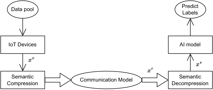
Figure 10: Process of Semantic Communication.

Furthermore, the reconstruction loss of a compression system follows the Gaussian distribution $\mathcal{N}(0,\sigma^{\text{sem}})$ [17]. Applying the gaussian distribution function with the lemma 1, the total variance for the sequential process of SemCom system is given by:

$$\sigma^{2}_{\text{tot}}=\sigma^{2}_{\text{sem}}+\sigma^{2}_{\text{model}}+\sigma^{2}_{\text{data}}$$ (47)

Appendix E Proof on Theorem 2

We consider the parameterized hypothesis class $\mathcal{H}=\{h_{\theta}|\theta\in\mathbf{R}^{d}\}$, where each member $h_{\theta}$ is a mapping from $\mathcal{X}_{i}$ to $\mathcal{Y}_{i}$ parameterized by $\theta$. With $z_{i}\triangleq(x_{i},y_{i})\in\mathcal{Z}_{i}$, we use $l(h(x_{i}),y_{i})$, shorthand for $l(h_{\theta}(x_{i}),y_{i})$, to represent the empirical distance between the ground truth $y_{i}$ and the predicted label $h_{\theta}(x_{i})$. Here, we consider empirical distance $l(h_{\theta}(x_{i}),y_{i})$ as Euclid distance which is represented as:

$$l(h_{\theta}(x_{i}),y_{i})=\|h_{\theta}(x_{i})-y_{i}\|$$ (48)

We also assume that the original data $x_{i}$ is the ideal data (i.e., center on its category of the global dataset) and the hypothesis is well-trained (i.e., the mapping function from $x_{i}\xrightarrow{h_{\theta}}y_{i}$ is correct with $100\%$ confidence).

Taking the hypothesis of distorted data $\hat{x}$ into consideration, we have the Taylor expansion of $h(\hat{x})$ up to the second-order equals to:

$$G(x) =\sum^{N}_{i=1}\ell(h(\hat{x}_{i}),y_{i})-\sum^{N}_{i=1}\ell(h(\widetilde{x}_{i}),y_{i})$$

$$=\sum^{N}_{i=1}\ell(\hat{x}_{i})-\sum^{N}_{i=1}\ell(\widetilde{x}_{i})$$

$$=\sum^{N}_{i=1}\ell(x_{i}+\sigma_{i})-\sum^{N}_{i=1}\ell(\widetilde{x}_{i})$$

$$\overset{(a)}{\leq}\sum^{N}_{i=1}\nabla\ell(x_{i})\sigma_{i}+\sum^{N}_{i=1}\frac{\nabla^{2}l(x_{i})}{2}\sigma_{i}^{2}$$

$$\leq\frac{L^{2}}{2}\sum^{N}_{i=1}\sigma_{i}^{2}\leq\frac{L^{2}}{2N}\widetilde{\sigma}^{2}.$$

Here, we denote $\widetilde{\sigma}$ as the variance of the global dataset $\mathcal{D}$ sampled from IoT devices. For simplicity, we define $\ell(h(x_{i}),y_{i})=\ell(x_{i})$. The inequality $(a)$ holds due to the assumption 3 of ideal data on well-train model $h^{*}_{\theta}$ (i.e., for all $x_{i},\exists\rho$ that satisfies $\nabla h^{*}_{\theta}(\widetilde{x_{i}})\leq\rho$.

Appendix F Proof on Theorem - Gradient Dissimilarity

We consider the gradient $\nabla F(\cdot)$ of data point $x_{i}$ as: $\nabla F(x_{i})$. When affected by the distortion, the data is distorted into $x+\sigma$, where $\sigma$ is the distortion rate of the data via the semantic channel. We have the following lagrange:

$$\nabla^{2}F(x)=\nabla\frac{F(x+\sigma)-\nabla f(x)}{(x+\sigma)-x}\leq L\mathbf{I}.$$ (49)

Therefore, we have:

$$\nabla F(x+\sigma)-\nabla F(x)\leq L\sigma.$$ (50)

Thus, we have the following gradient dissimilarity:

$$\nabla F(x+\sigma)\leq\nabla F(x)+L\sigma.$$ (51)

Therefore, we have:

$$\|\nabla F(x+\sigma)\|^{2}\leq\|\nabla F(x)+L\sigma\|^{2}$$ (52)

Appendix G Proof on Theorem - Gradient Inductive

We consider the gradient of distorted data $\hat{x}=x+\sigma$ as $F(\cdot;\hat{x)}$. For ease of the proof, we denote $F(\cdot;\hat{x)}=F(w^{n})$, where $w^{n}$ is the model parameters $w$ at iteration $n$. We have the followings:

$$F(w^{n+1};\hat{x})=F(w^{n+1})=F[w^{n}-\eta\nabla F(w^{n})]$$

$$=F(w^{n})-\eta\|\nabla F(w^{n})\|^{2}+\frac{\eta^{2}}{2}\|\nabla F(w^{n})\|^{2}\cdot\nabla^{2}F(w^{n})$$

$$\leq F(w^{n})-\eta\|\nabla F(w^{n})\|^{2}+\eta^{2}\frac{L}{2}\|\nabla F(w^{n})\|^{2}$$

$$=F(w^{n})+\left(\eta^{2}\frac{L}{2}-\eta\right)\|\nabla F(w^{n})\|^{2}.$$ (53)

Hehe according to L-smooth

$$F(w^{n+1};\hat{x})\leq F(w^{n};\hat{x})+\left(\eta^{2}\frac{L}{2}-\eta\right)\|\nabla F(w^{n};\hat{x})\|^{2}$$ (54)

$$\leq F(w^{n};\hat{x})+\left(\eta^{2}\frac{L}{2}-\eta\right)\|\nabla F(w^{n};x)+L\sigma\|^{2}$$

And hehe according to $\mu$-convex

$$F(w^{n+1};\hat{x})\geq F(w^{n};\hat{x})+\left(\eta^{2}\frac{\mu}{2}-\eta\right)\|\nabla F(w^{n};\hat{x})\|^{2}$$ (55)

$$\geq F(w^{n};\hat{x})+\left(\eta^{2}\frac{\mu}{2}-\eta\right)\|\nabla F(w^{n};x)+L\sigma\|^{2}$$

Taking the Generalization Gap into consideration, we have the followings:

$$F (w^{n+1};\hat{x})-F(w^{n+1};x)$$

$$\leq \left[F(w^{n};\hat{x})+\left(\eta^{2}\frac{L}{2}-\eta\right)\|\nabla F(w^{n};\hat{x})\|^{2}\right]$$

$$- \left[F(w^{n};x)+\left(\eta^{2}\frac{\mu}{2}-\eta\right)\|\nabla F(w^{n};x)\|^{2}\right]$$

$$\leq \left[F(w^{n};\hat{x})-F(w^{n};x)\right]$$

$$+ \left[\left(\eta^{2}\frac{L}{2}-\eta\right)\|\nabla F(w^{n};\hat{x})\|^{2}-\left(\eta^{2}\frac{\mu}{2}-\eta\right)\|\nabla F(w^{n};x)\|^{2}\right]$$

$$\leq \left[F(w^{n};\hat{x})-F(w^{n};x)\right]$$

$$+ \left[\left(\eta^{2}\frac{L}{2}-\eta\right)\|\nabla F(w^{n};x)+L\sigma\|^{2}\right.$$

$$-\left.\left(\eta^{2}\frac{\mu}{2}-\eta\right)\|\nabla F(w^{n};x)\|^{2}\right]$$

$$\leq \left[F(w^{n};\hat{x})-F(w^{n};x)\right]$$

$$+ \left[\left(\eta^{2}\frac{L}{2}-\eta\right)\left[\|\nabla F(w^{n};x)\|^{2}+\|L\sigma\|^{2}\right]\right.$$

$$-\left.\left(\eta^{2}\frac{\mu}{2}-\eta\right)\|\nabla F(w^{n};x)\|^{2}\right]$$

$$\leq \left[F(w^{n};\hat{x})-F(w^{n};x)\right]$$ (56)

$$+ \left[\left(\eta^{2}\frac{L}{2}-\eta\right)\|L\sigma\|^{2}+\frac{\eta^{2}}{2}\left(L-\mu\right)\|\nabla F(w^{n};x)\|^{2}\right].$$

By choosing the $L$-smooth and $\mu$-strongly convex such that $L=\mu$, we have:

$$R(w^{n})=F(w^{n};\hat{x})-F(w^{n};x)$$

$$\leq F(w^{n-1};\hat{x})-F(w^{n-1};x)+\left(\eta^{2}\frac{L}{2}-\eta\right)(L\sigma)^{2}$$

$$=F(w^{0};\hat{x})-F(w^{0};x)+n\left(\eta^{2}\frac{L}{2}-\eta\right)(L\sigma)^{2}.$$ (57)

Here, we have $F(w^{0};\hat{x})=F(w^{0};x)$ (because at the initial weight $w^{0}$, the loss on two data is equivalent). Thus, we have:

$$F(w^{n};\hat{x})-F(w^{n};x)\leq n\left(\eta^{2}\frac{L}{2}-\eta\right)(L\sigma)^{2}.$$ (58)

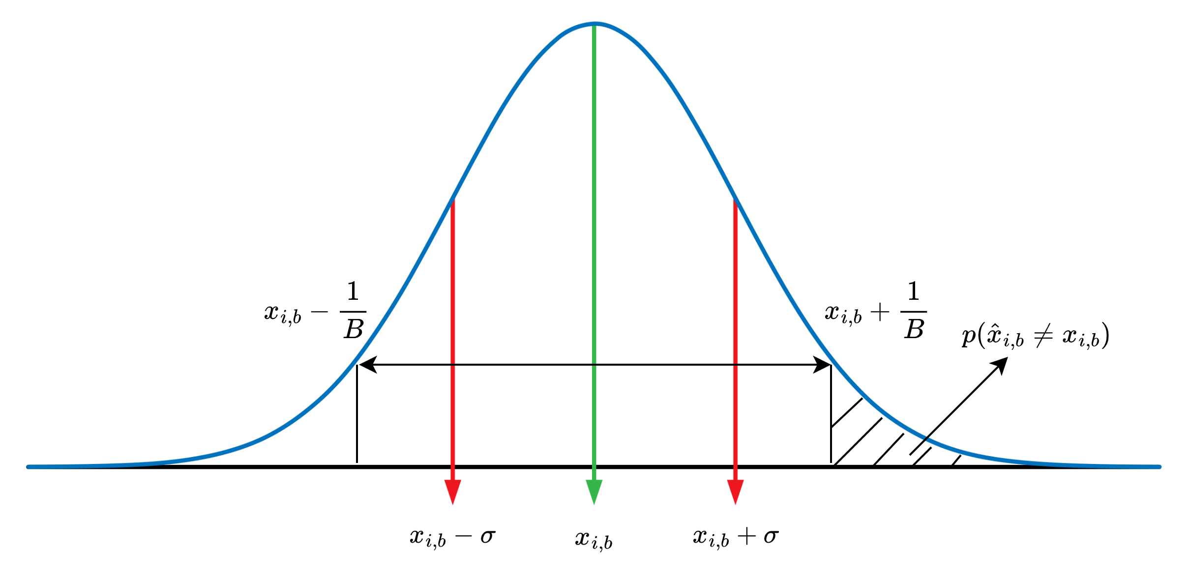
Figure 11: Illustration on Probability Decision Boundary induced by Gaussian noise.

Appendix H Proof on Lemma - Total Variation

$$\textrm{TV}(\mathbf{x},\mathbf{\hat{x}}) =\underset{v\in\mathcal{V}}{\textrm{sup}}\left[P(x)-P(\hat{x})\right]$$

$$=\underset{v\in\mathcal{V}}{\textrm{sup}}\left[\underset{\mathbf{x}\in\mathcal{X}}{\int}p(x)dx-\underset{\mathbf{x}\in\mathcal{X}}{\int}q(x)dx)\right]$$

$$=\underset{v\in\mathcal{V}}{\textrm{sup}}\left[\underset{\mathbf{x}\in\mathcal{X}}{\int}\langle p(x)-q(x)\rangle dx\right].$$ (59)

Here, we have the transportation policy $v$ is sampled from the set of possible transportation policy $\mathcal{V}$. As mentioned in [18], the input $p(x_{i})$ is model by the set of $p(x_{i,b})$ where $b$ is the bit index in the data $i$. Therefore, we can have the followings:

$$\textrm{TV}(\mathbf{x},\mathbf{\hat{x}}) =\underset{v\in\mathcal{V}}{\textrm{sup}}\left|P(x)-P(\hat{x})\right|$$

$$=\underset{v\in\mathcal{V}}{\textrm{sup}}\left[\underset{x\in\mathbf{x}}{\int}|p(x)-q(x)|dx\right]$$

$$=\overset{|x|}{\underset{i=0}{\sum}}\overset{B}{\underset{b=0}{\sum}}|p(x_{i,b})-p(\hat{x}_{i,b})|,$$ (60)

where $p(x_{i,b}),p(\hat{x}_{i,b})$ represent the element-wise probability of the data $x_{i}$ and $\hat{x}_{i}$ at bit index $b$, respectively. To be more specific, $p(x_{i,b})$ indicates the probability that bit $x_{i}$ is $1$. Due to the distortion effect, decision boundary of the data can be moved by noise $v\sim\mathcal{N}(0,\sigma^{2})$, where $\sigma^{2}$ is the variance of the Gaussian noise with mean $0$. We have the variance can be represented as:

$$\sigma^{2} =\frac{1}{NB}\sum^{N}_{i=1}\sum^{B}_{b=1}(x_{i,b}-\hat{x}_{i,b})^{2}=MSE(x_{i},\hat{x}_{i})$$ (61)

Thus, we can have the data point being induced by the Gaussian noise can be represented as Figure 11. Thus, we have the probability of $p(x_{i,b})-p(\hat{x}_{i,b}=x_{i,b})=p(\hat{x}_{i,b}\neq p(x_{i,b}))$. Therefore, we can have the followings:

$$p(x_{i,b})-p(\hat{x}_{i,b})=p(\hat{x}_{i,b}\neq x_{i,b})=p(\frac{v}{\sigma^{2}}\geq W)$$

$$=\int^{\infty}_{W}\frac{1}{\sqrt{2\pi}\sigma}e^{-\left(\frac{x}{2\sigma}\right)^{2}}\leq\frac{1}{\sqrt{2\pi}\sigma}e^{-\left(\frac{W}{2\sigma}\right)^{2}}$$ (62)

Appendix I Proof on Theorem - Inference Divergence

We consider the gradient of distorted data $\hat{x}=x+\sigma$ as $F(\cdot;\hat{x)}$. For ease of the proof, we denote $F(\cdot;\hat{x)}=F(w^{n})$, where $w^{n}$ is the model parameters $w$ at iteration $n$. We have the followings:

$$p(\mathbf{\hat{t}}) =p(\mathbf{t}|\mathbf{\hat{s}})p(\mathbf{\hat{s}})=p(\mathbf{t}|\mathbf{s})p(\mathbf{\hat{s}})$$ (63)

We consider the long-term performance of the SemCom system. Thus, we consider the expected output as follows:

$$\mathbb{E}\left[p(\mathbf{\hat{t}})\right] =\mathbb{E}\left[p(\mathbf{t}|\mathbf{s})p(\mathbf{\hat{s}})\right]$$

$$=\mathbb{E}\left[p(\mathbf{t}|\mathbf{s})p(\mathbf{s})\right]+\mathbb{E}\left[p(\mathbf{t}|\mathbf{s})\langle p(\mathbf{\hat{s}})-p(\mathbf{s})\rangle\right]$$

$$=\mathbb{E}\left[p(\mathbf{t})\right]+p(\mathbf{t}|\mathbf{s})\mathbb{E}\left[p(\mathbf{\hat{s}})-p(\mathbf{s})\right].$$ (64)

Applying the inequality in Lemma 3, we have the following:

$$\mathbb{E}\left[p(\mathbf{\hat{t}})-p(\mathbf{t})\right] \leq\frac{1}{\sqrt{2\pi}\sigma}p(\mathbf{t}|\mathbf{s})\exp{-\left(\frac{W}{2\sigma}\right)^{2}}.$$ (65)

Appendix J Proof on Theorem - Domain Aggregation

$$\sigma^{2}_{\textrm{tot}} =MSE(x_{i},\hat{x}_{i})$$

$$=\|x_{i,b}-\hat{x}_{i,b}\|^{2}_{2}=\mathbb{E}[(x-\mu)^{2}]=\mathbb{E}[x^{2}]$$

$$=\mathbb{E}_{u\in U}\left[\mathbb{E}_{x\in X_{u}}[x^{2}]\right]$$

$$=\frac{1}{\sum^{U}_{u=1}D_{u}}\sum D_{u}\mathbb{E}_{x\in X_{u}}[x^{2}]$$

$$=\frac{1}{D}\sum^{U}_{u=1}D_{u}\sigma^{2}_{\textrm{tot},u}$$ (66)

References

- [1] W. Y. B. Lim, N. C. Luong, D. T. Hoang, Y. Jiao, Y.-C. Liang, Q. Yang, D. Niyato, and C. Miao, “Federated learning in mobile edge networks: A comprehensive survey,” IEEE Communications Surveys & Tutorials, vol. 22, no. 3, pp. 2031–2063, Apr. 2020.
- [2] D. T. Hoang, C. Lee, D. Niyato, and P. Wang, “A survey of mobile cloud computing: architecture, applications, and approaches.” Wirel. Commun. Mob. Comput., vol. 13, no. 18, pp. 1587–1611, 2013. [Online]. Available: http://dblp.uni-trier.de/db/journals/wicomm/wicomm13.html#HoangLNW13
- [3] L. Zhang, Y.-C. Liang, and D. Niyato, “6g visions: Mobile ultra-broadband, super internet-of-things, and artificial intelligence,” China Communications, vol. 16, no. 8, pp. 1–14, 2019.
- [4] T. Huynh-The, Q.-V. Pham, X.-Q. Pham, T. T. Nguyen, Z. Han, and D.-S. Kim, “Artificial intelligence for the metaverse: A survey,” Engineering Applications of Artificial Intelligence, vol. 117, p. 105581, 2023. [Online]. Available: https://www.sciencedirect.com/science/article/pii/S0952197622005711
- [5] Q. Lan, D. Wen, Z. Zhang, Q. Zeng, X. Chen, P. Popovski, and K. Huang, “What is semantic communication? a view on conveying meaning in the era of machine intelligence,” Journal of Communications and Information Networks, vol. 6, no. 4, pp. 336–371, 2021.
- [6] W. Xu, Z. Yang, D. W. K. Ng, M. Levorato, Y. C. Eldar, and M. Debbah, “Edge learning for b5g networks with distributed signal processing: Semantic communication, edge computing, and wireless sensing,” IEEE Journal of Selected Topics in Signal Processing, vol. 17, no. 1, pp. 9–39, Jan. 2023.
- [7] Z. Qin, X. Tao, J. Lu, W. Tong, and G. Y. Li, “Semantic communications: Principles and challenges,” 2022. [Online]. Available: https://arxiv.org/abs/2201.01389
- [8] D. Gündüz, Z. Qin, I. E. Aguerri, H. S. Dhillon, Z. Yang, A. Yener, K. K. Wong, and C.-B. Chae, “Beyond transmitting bits: Context, semantics, and task-oriented communications,” IEEE Journal on Selected Areas in Communications, vol. 41, no. 1, pp. 5–41, April. 2023.
- [9] H. Xie, Z. Qin, G. Y. Li, and B.-H. Juang, “Deep learning enabled semantic communication systems,” IEEE Transactions on Signal Processing, vol. 69, pp. 2663–2675, 2021.
- [10] T. Han, Q. Yang, Z. Shi, S. He, and Z. Zhang, “Semantic-aware speech to text transmission with redundancy removal,” 2022. [Online]. Available: https://arxiv.org/abs/2202.03211
- [11] L. Yan, Z. Qin, R. Zhang, Y. Li, and G. Y. Li, “Resource allocation for text semantic communicationsb,” 2022. [Online]. Available: https://arxiv.org/abs/2201.06023
- [12] C. Liu, C. Guo, Y. Yang, and N. Jiang, “Adaptable semantic compression and resource allocation for task-oriented communications,” 2022. [Online]. Available: https://arxiv.org/abs/2204.08910
- [13] C. Liu, C. Guo, Y. Yang, and J. Chen, “Bandwidth and power allocation for task-oriented semanticcommunication,” 2022. [Online]. Available: https://arxiv.org/abs/2201.10795
- [14] W. C. Ng, H. Du, W. Y. B. Lim, Z. Xiong, D. Niyato, and C. Miao, “Stochastic resource allocation for semantic communication-aided virtual transportation networks in the metaverse,” 2022. [Online]. Available: https://arxiv.org/abs/2208.14661
- [15] L. Yan, Z. Qin, R. Zhang, Y. Li, and G. Y. Li, “Qoe-aware resource allocation for semantic communication networks,” 2022. [Online]. Available: https://arxiv.org/abs/2205.14530
- [16] Z. Yang, M. Chen, Z. Zhang, and C. Huang, “Energy efficient semantic communication over wireless networks with rate splitting,” IEEE Journal on Selected Areas in Communications, vol. 41, no. 5, pp. 1484–1495, 2023.
- [17] M.-D. Nguyen, S.-M. Lee, Q.-V. Pham, D. T. Hoang, D. N. Nguyen, and W.-J. Hwang, “Hcfl: A high compression approach for communication-efficient federated learning in very large scale iot networks,” IEEE Transactions on Mobile Computing, pp. 1–13, Jul. 2022.
- [18] Y. Bengio, P. Lamblin, D. Popovici, H. Larochelle et al., “Greedy layer-wise training of deep networks,” Advances in neural information processing systems, vol. 19, p. 153, Dec. 2006.
- [19] S. Boyd and L. Vandenberghe, Convex Optimization. Cambridge University Press, March 2004. [Online]. Available: http://www.amazon.com/exec/obidos/redirect?tag=citeulike-20&path=ASIN/0521833787
- [20] A. Krizhevsky, “Learning multiple layers of features from tiny images,” Tech. Rep., Aug. 2009.
- [21] L. Dinh, R. Pascanu, S. Bengio, and Y. Bengio, “Sharp minima can generalize for deep nets,” in Proceedings of the 34th International Conference on Machine Learning, ser. Proceedings of Machine Learning Research, D. Precup and Y. W. Teh, Eds., vol. 70. PMLR, 06–11 Aug 2017, pp. 1019–1028.
- [22] P. Goyal, P. Dollár, R. Girshick, P. Noordhuis, L. Wesolowski, A. Kyrola, A. Tulloch, Y. Jia, and K. He, “Accurate, large minibatch sgd: Training imagenet in 1 hour,” 2018.
- [23] Y. You, J. Li, S. Reddi, J. Hseu, S. Kumar, S. Bhojanapalli, X. Song, J. Demmel, K. Keutzer, and C.-J. Hsieh, “Large batch optimization for deep learning: Training bert in 76 minutes,” in International Conference on Learning Representations, 2020.