Achieving Autonomous Cloth Manipulation with Optimal Control via Differentiable Physics-Aware Regularization and Safety Constraints

Abstract

Cloth manipulation is a category of deformable object manipulation of great interest to the robotics community, from applications of automated laundry-folding and home organizing and cleaning to textiles and flexible manufacturing. Despite the desire for automated cloth manipulation, the thin-shell dynamics and under-actuation nature of cloth present significant challenges for robots to effectively interact with them. Many recent works omit explicit modeling in favor of learning-based methods that may yield control policies directly. However, these methods require large training sets that must be collected and curated. In this regard, we create a framework for differentiable modeling of cloth dynamics leveraging an Extended Position-based Dynamics (XPBD) algorithm. Together with the desired control objective, physics-aware regularization terms are designed for better results, including trajectory smoothness and elastic potential energy. In addition, safety constraints, such as avoiding obstacles, can be specified using signed distance functions (SDFs). We formulate the cloth manipulation task with safety constraints as a constrained optimization problem, which can be effectively solved by mainstream gradient-based optimizers thanks to the end-to-end differentiability of our framework. Finally, we assess the proposed framework for manipulation tasks with various safety thresholds and demonstrate the feasibility of result trajectories on a surgical robot. The effects of the regularization terms are analyzed in an additional ablation study.

I INTRODUCTION

Cloth manipulation has numerous applications both in housework and manufacturing for robotics, but it remains challenging due to the material’s deformable, flexible, and dynamic nature. The manipulation of cloth can be seen as an overall trajectory planning process with a focus on changing the shape configuration while maintaining geometrical or topological properties. Unlike rigid objects, cloth is difficult to manipulate due to the under-actuated control with infinite degrees of freedom for shape deformation. Meanwhile, slight disturbances on cloth can result in significantly dynamic behaviors, such as bending, crumpling, and self-occlusion [1]. Study into cloth manipulation in the robotics community has covered various aspects, including visual representation [2], latent-space modeling [3], cloth grasping primitive [4], sequential multi-step control [5], imitation learning [6] and reinforcement learning [7].

Trajectories play a pivotal role in addressing multiple safety-critical tasks. In contrast to rigid objects, cloth dynamics exhibit diverse responses influenced by their interactions with the environment, primarily through deformation. Consequently, incorporating considerations of reliability and safety into cloth control poses a significant challenge for modeling and planning. Even with the integration of a high-fidelity deformable model for cloth with constraints, the task of trajectory optimization remains challenging [8, 9, 10].

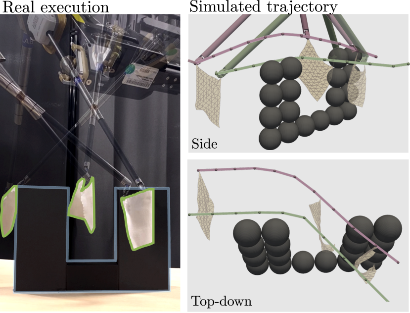
Figure 1: Execution of an optimized physics-aware and safe cloth manipulation trajectory in real work on a dVRK system (left) and in a XPBD simulation with robot kinematics (right). The obstacles are represented with spheres in the simulator. We show that we can make the cloth follow trajectories through constrained environments while achieving goal configurations under dynamic motion.

Therefore, our objective is to build a physics-based approach for manipulating cloth that can generate control trajectories while taking into account both the dynamics of cloth and regulations of trajectories for safety. The ideal control sequence should ensure the cloth to a target position through a smooth trajectory without overstretching the cloth or breaking safety constraints.

I-A Contributions

In recent years, simulations of deformable objects have been increasingly developed in the field of Computer Graphics. By simply defining various geometrical constraints, position-based dynamics (PBD) has proven to be a promising method for fast online simulation of deformable objects [11, 12, 13, 14, 15]. Based on the extended position-based dynamics (XPBD) algorithm [16], we propose a framework for cloth manipulation that regularizes physics-aware metrics and complies with safety constraints. To this end, we present the following novel contributions :

• We leverage the full differentiability of the developed XPBD simulation to power a gradient-based trajectory optimization framework for cloth manipulation.

• Physics-aware regularization terms are introduced and integrated into our framework to prevent undesired behaviors, such as over-stretching and wrinkling.

• Safety constraints such as obstacle avoidance requirements are formulated as a constraint function that can be incorporated into the trajectory optimization framework.

• We evaluate the framework with non-trivial cloth manipulation tasks. Different metrics are extensively analyzed and the trajectory is executed by the dVRK robot to verify its compatibility with real robot kinematics.

II Related Works

II-A Cloth Dynamics Modeling

Research in cloth dynamics, explored in computer graphics and robotics, encompasses various modeling techniques, from mass-spring systems to FEM-based continuum mechanics [17, 9]. These models have informed cloth manipulation strategies for motion controllers [18, 19], but can be challenged by complex environments and local minima.

Recently, deep learning has driven interest in data-driven approaches. One group employs neural networks to create cloth dynamics models, applying latent space control [2, 3, 20]. Another group uses model-free methods, such as deep imitation learning [6, 21, 22], dynamic movement primitives [23, 24], and reinforcement learning [7, 25, 26], often based on trial-and-error in simulation. However, these methods may face challenges with implicit models and costly real robot training with defined reward functions.

II-B Safe Manipulation

In recent years, robotics has focused on safety planning and control, driven by methods like control barrier functions (CBFs) [27, 28, 29]. However, these methods mainly apply to rigid robots, addressing safety constraints like contact forces and joint limits. Research spans legged robot locomotion [30, 31] and robotic manipulators [32, 33].

Conversely, cloth manipulation, particularly with a safety focus, has seen limited exploration. Recent work primarily adopts learning-based approaches for safe manipulation policies [34, 35] and learning to ensure safe interactions between cloth and its environment [36, 37]. Notably, Erickson et al. [38] demonstrated using learned models for safe model predictive control. However, these methods rely on substantial training data, which could benefit from incorporating physics simulations.

III Methodology

III-A Problem Formulation

The state of the cloth is given by $\mathbf{x}\in\mathbb{R}^{N\times 3}$, where $N$ is the number of particles in the cloth mesh. At each time step $t$, $\mathbf{x}^{(t)}$ can be computed from previous state $\mathbf{x}^{(t-1)}$ by applying control $\mathbf{u}^{(t-1)}$. The control sequence $\mathbf{U}$ is characterized as a list of displacement vectors associated with specific control points. Given control sequence $\mathbf{U}=[\mathbf{u}^{(0)},\mathbf{u}^{(2)},\dots,\mathbf{u}^{(T-1)}]^{\top}$ and initial state $\mathbf{x}^{init}$, we can obtain a sequence of intermediate states $\mathbf{X}=[\mathbf{x}^{(1)},\mathbf{x}^{(2)},\dots,\mathbf{x}^{(T)}]^{\top}$. Then, the cloth manipulation task can be formulated as a trajectory optimization problem, given by:

$$\arg\min_{\mathbf{U}} \mathcal{L}(\mathbf{X},\mathbf{U})$$ (1)

s.t. $$\mathbf{x}^{(t)}=\mathcal{XPBD}\left(\mathbf{x}^{(t-1)},\mathbf{u}^{(t-1)}\right)$$

$$\mathbf{x^{(0)}}=x^{init}$$

$$\mathcal{C}(\mathbf{X})\geq 0$$

where $\mathcal{L}$ is the objective function that includes error and regularization terms, $\mathcal{XPBD}$ represents the extended position-based dynamics algorithm [16], and $\mathcal{C}$ specifies safety constraints on all intermediate states of the cloth.

III-B XPBD Simulation

PBD [11] is a physics simulation algorithm based on geometric constraints and positional updates that models deformable objects as a discrete system with particles. Compared with traditional force-based methods, PBD is more stable and controllable and converges orders-of-magnitude faster than force-based methods. These benefits make PBD widely used in real-time interactive scenarios. XPBD [16] is an extension to the original PBD algorithm to address the issue of iteration and time step-dependent stiffness. It also builds the connection between geometric constraints and elastic potential energy. Later, we will use this physical interpretation to formulate a regularization term that constrains undesired cloth deformation.

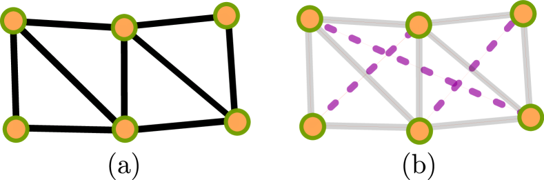
Figure 2: Visualization of distance and bending constraints in particle-mesh structure. $(a)$ A triangular mesh with particles and edges. $(b)$ Distance constraints (gray solid line) and bending constraints (purple dashed line).

In this work, we implement a quasi-static XPBD simulation to simulate the state of the cloth under a slow-moving control sequence. In a quasi-static process, the state of the cloth evolves from one state to another infinitesimally slowly, ensuring that it always remains in equilibrium. From this assumption, velocity terms can be ignored. We use distance and bending constraints to model the thin-shell deformation of cloth, as shown in Fig. 2.

• Distance Constraint $\mathbf{C}_{dist}(\mathbf{x_{i}},\mathbf{x_{j}})$ is defined between each pair of connected particles in each triangle.

• Bending Constraint $\mathbf{C}_{bend}(\mathbf{x_{i}},\mathbf{x_{j}})$ is defined between each pair of non-neighboring particles in each pair of adjacent triangles.

The shared constraint function is identically defined as:

$$\mathbf{C}_{dist/bend}(\mathbf{x}_{i},\mathbf{x}_{j})=\|\mathbf{x}_{i}-\mathbf{x}_{j}\|-\mathbf{d}^{0}_{ij}$$ (2)

where $\mathbf{d}^{0}_{ij}$ is the initial distance between $\mathbf{x}_{i}$ and $\mathbf{x}_{j}$. More details of these constraint functions and their gradients can be found in [11].

We adopt the Gauss-Seidel style solver [39], where the result from one constraint projection is used in the next constraint projection, as it exhibits good convergence and stability. To parallelize the constraint projection steps while avoiding data race conditions, we separate constraints into independent sets where there is no particle shared by any constraint, as shown in Fig. 3. We can then efficiently project each set of constraints in parallel with broadcast syntax.

Figure 3: An example of constructing independent sets of constraints. In this example mesh, distance constraints are grouped into four independent sets labeled with different colors. In each set, there is no particle that is shared by any constraint. Therefore, the constraint projection in each set can be done in parallel to speed up the simulation.

III-C Objective Function and Safety Constraints

We define the terminal objective of the trajectory optimization problem as positional alignments between a subset of simulation particles $\mathbf{\bar{x}}\subset\mathbf{x}^{(T)}$ and some user-defined target position $\mathbf{x}_{target}$. The target error is the $L_{2}$ distance between the subset of particles and the target position.

$$\mathcal{G}(\mathbf{x}^{(T)},\mathbf{x}_{target})=\|\mathbf{x}_{target}-\mathbf{\bar{x}}\|$$ (3)

By only considering the terminal alignment of particles, the framework may generate irregular trajectories inducing excessive deformation on intermediate states of the cloth. To ensure the smoothness of the trajectory $\mathbf{U}$, the difference between two neighboring control vectors should be limited. Therefore, we regularize the trajectory irregularity as the sum of the backward difference of the control sequence in discrete time steps.

$$\small\mathcal{T}(\mathbf{U})=\sum\nolimits_{t=1}^{T}\|\mathbf{u}_{i}-\mathbf{u}_{i-1}\|$$ (4)

We emphasize that an optimal control sequence is aware of the deformation physics of the cloth, preventing undesirable overstretching and bending effects. This can be accomplished by regularizing the potential energy of the cloth over time. In our XPBD simulation, the total potential energy is the sum of the energy of every geometric constraint. Let $\mathbf{C}(\mathbf{\mathbf{x}^{(t)}})=[C_{1}(\mathbf{\mathbf{\mathbf{x}^{(t)}}}),C_{2}(\mathbf{\mathbf{\mathbf{x}^{(t)}}}),\dots,C_{m}(\mathbf{\mathbf{x}^{(t)}})]^{\top}$ be a set of geometric constraints, and let $\mathbf{K}=[k_{1},k_{2},\dots,k_{m}]^{T}$ be their associated stiffness parameters. The potential energy of the cloth through the control trajectory can be expressed as:

$$\small\begin{split}\mathcal{E}(\mathbf{X})=\sum\nolimits_{t=1}^{T}\large\nicefrac{{1}}{{2}}\ \mathbf{C}(\mathbf{x}^{(t)})^{\top}\mathtt{diag}(\mathbf{K})\mathbf{C}(\mathbf{x}^{(t)})\end{split}$$ (5)

The objective function is then the combination of target error, trajectory irregularity and potential energy regularization:

$$\begin{split}\mathcal{L}(\mathbf{X},\mathbf{U})=\mathcal{G}(\mathbf{x}^{(T)},\mathbf{x}_{target})+\alpha\mathcal{T}(\mathbf{U})+\beta\mathcal{E}(\mathbf{X})\end{split}$$ (6)

Here, $\alpha$ and $\beta$ are scaling coefficients on two regularization terms. Later we will study the effects of the regularization terms in an ablation study.

Safety constraints are essential in many manipulation tasks. Our formulation 1 allows us to incorporate various safety constraints, such as robot joint limit, contact forces, and obstacle avoidance, into the differentiable simulation framework. For simplicity, we demonstrate its ability in an obstacle avoidance scenario. The distance to the obstacle can be specified by an SDF $\mathcal{SDF}$ where a positive value means outside and a negative value means inside. To simplify the computation of the SDF, we approximate different obstacle shapes with numerous spheres. For a sphere $\mathbf{s}$ centered at point $\mathbf{c}$ with radius $r$, the SDF can be written as:

$$\mathcal{SDF}_{\mathbf{s}}(\mathbf{x})=\|\mathbf{x}-\mathbf{c}\|-r$$ (7)

The SDF of the entire obstacle is then given by:

$$\mathcal{SDF}(\mathbf{x})=\min\{\mathcal{SDF}_{\mathbf{s}}(\mathbf{x})\text{ for }\mathbf{s}\in\mathbf{S}\}$$ (8)

where $\mathbf{S}$ is the set of spheres making up the obstacle. This approximation is highly popular in robotic planning applications and in solving for feasible inverse-kinematic solutions in constrained environments. Furthermore, the fact that it is analytically and efficiently evaluated is beneficial to the optimization procedure. We refer readers to Diffco [40] for an alterative still-differentiable SDF formulation that goes beyond spherical approximation for generality and is still computationally efficient for trajectory optimization.

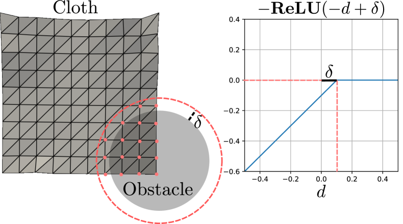
Figure 4: Illustration of the collision constraint. On the left, the cloth penetrates the gray obstacle. The red dashed circle indicates the range of collision avoidance shifted by the constant $\delta$. All the particles result in negative constraint values are marked by the red dots. On the right, we plot the function $-\mathbf{ReLU}(-d+\delta)$. It is clear that the function value is negative for all $d<\delta$, which is up to our control.

We can record the signed distance $d_{i}^{(t)}=\mathcal{SDF}(\mathbf{x}_{i}^{(t)})$ of each particle at each time step. Then, a constant $\delta>0$ is subtracted from all signed distances, which gives us flexible control of how far we want to avoid the obstacle. To collect all values violating the safety constraint, we modify the widely used Rectified Linear Unit ($\mathbf{ReLU}$) function. Considering function $-\mathbf{ReLU}(-d+\delta)$, the value will be $d-\delta$ when $d$ is smaller than $\delta$, $0$ when $d$ is no less than $\delta$. We can then express our obstacle avoidance safety constraint as the sum of all the particles along the control trajectory.

$$\small\mathcal{C}(\mathbf{X})=\sum\nolimits_{t=1}^{T}\sum\nolimits_{i=1}^{N}-\textbf{ReLU}(-d_{i}^{(t)}+\delta)$$ (9)

This constraint function would be non-negative only when signed distances of all particles are no less than threshold $\delta$. Fig 4 visualizes an example collision and plots the behavior of the modified $\mathbf{ReLU}$ function we use in the constraint.

1

Input : Initial state $\mathbf{x}^{(0)}$,initial control sequence $\mathbf{U}$, distance stiffness $\mathbf{k}_{dis}$, bending stiffness $\mathbf{k}_{bend}$

Output : Optimized control sequence $\mathbf{U}^{*}$

2 for $t$ in $1...T$ do

3      

4      $\mathbf{x}^{(t)}\leftarrow\mathbf{x}^{(t-1)}+\frac{1}{2}\mathbf{g}\Delta{t}^{2}$

5      $\mathbf{x}^{(t)}\leftarrow\mathtt{applyControl}\left(\mathbf{x}^{(t)},\mathbf{u}^{(t-1)}\right)$

      // Constraints solving loop

6       while iter $<$ iteration do

             // Solve distance and bending (Eq. 2)

7             $\Delta{\mathbf{x}_{dis}}\leftarrow\mathtt{solveDistance}\left(\mathbf{C}_{dist}\left(\mathbf{x}^{(t+1)}\right),\mathbf{k}_{dis}\right)$

8            $\Delta{\mathbf{x}_{bend}}\leftarrow\mathtt{solveBending}\left(\mathbf{C}_{bend}\left(\mathbf{x}^{(t+1)}\right),\mathbf{k}_{bend}\right)$

            // Update cloth state

9             $\mathbf{x}^{(t)}\leftarrow\mathbf{x}^{(t)}+\Delta{\mathbf{x}_{dis}}+\Delta{\mathbf{x}_{bend}}$

      // Compute time step gradient

10       $\nabla\mathcal{XPBD}\leftarrow\displaystyle\large\nicefrac{{\partial\mathbf{x}^{(t)}}}{{\partial\mathbf{u}^{(t-1)}}}$

11

12$\mathbf{X}\leftarrow\mathbf{x}^{(0)},\cdots,\mathbf{x}^{(T)}$

// Obtain the loss function

13 $\mathcal{L}\leftarrow\mathcal{L}\left(\mathbf{X},\mathbf{U}\right)$

// Obtain the safety constraint function

14 $\mathcal{C}\leftarrow\mathcal{C}\left(\mathbf{X}\right)$

// Compute optimized control

$\mathbf{U}^{*}\leftarrow\mathtt{optimizer}\left(\mathcal{L},\frac{d\mathcal{L}}{d\mathbf{U}},\mathcal{C}\right)$

Algorithm 1 Differentiable $\mathcal{XPBD}$ Cloth Manipulation Framework

III-D Differentiation Framework

To find the control sequence through optimization, it is necessary to compute the gradient of the objective function with respect to $\mathbf{U}$. Given objective function function $\mathcal{L}(\mathbf{X},\mathbf{U})$, by chain rule we have:

$$\frac{\mathrm{d}\mathcal{L}}{\mathrm{d}\mathbf{U}}=\frac{\partial\mathcal{L}}{\partial\mathbf{U}}+\frac{\partial\mathcal{L}}{\partial\mathbf{X}}\frac{\mathrm{d}\mathbf{X}}{\mathrm{d}\mathbf{U}}$$ (10)

We can perform gradient-based optimization using Newton or quasi-Newton methods [41] [42]. It should be noticed that the challenge is to evaluate the total derivative $\frac{\mathrm{d}\mathbf{X}}{\mathrm{d}\mathbf{U}}$. According to the XPBD system in Eq. 1, each Jacobian element in the total derivative can be expressed by:

$$\left[\frac{\mathrm{d}\mathbf{X}}{\mathrm{d}\mathbf{U}}\right]^{(p,q)}=\frac{\mathrm{d}\mathbf{x}^{(p)}}{\mathrm{d}\mathbf{u}^{(q)}}$$ (11)

where

$$\small\frac{\mathrm{d}\mathbf{x}^{(p)}}{\mathrm{d}\mathbf{u}^{(q)}}=\left\{\begin{aligned} &\frac{\partial\mathbf{x}^{(p)}}{\partial\mathbf{x}^{(p-1)}}\frac{\mathrm{d}\mathbf{x}^{(p-1)}}{\mathrm{d}\mathbf{u}^{(q)}},~{}~{}~{}~{}~{}\quad\quad q<p-1\\[3.87498pt] &\nabla_{\mathbf{u}}\mathcal{XPBD}\mid_{(\mathbf{x}^{(p-1)},\mathbf{u}^{(p-1)})},q=p-1\\[3.87498pt] &0,\qquad\qquad\qquad\qquad\qquad\text{otherwise}\end{aligned}\right.$$ (12)

Therefore, it is clear that all we need to do is to compute $\nabla_{\mathbf{u}}\mathcal{XPBD}$ iteratively at each time step.

We detailed our differentiable XPBD simulation in Algorithm 1. It is implemented as a PyTorch differentiation layer by subclassing the torch.autograd.Function. This enables us to back-propagate from any state $\mathbf{x}^{(p)}$ and compute its derivative with respect to past control input $\mathbf{u}^{(q)}$. The derivatives regarding objective function $\frac{\partial\mathcal{L}}{\partial\mathbf{U}}$ and $\frac{\partial\mathcal{L}}{\partial\mathbf{X}}$ are also calculated using auto-differentiation operations, so the entire computation process is end-to-end differentiable.

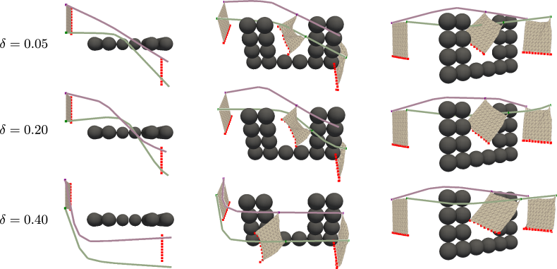
Figure 5: Visualizations of optimized manipulation trajectories with different safety thresholds $\delta$. Each row illustrates the trajectory with a safety threshold from different viewing angles. Red points denote the target position and the involved particles on the cloth. The purple and green lines are the paths of the two control points under the manipulation trajectory. The leftmost column only plots the initial state of the cloth. The right two columns show the initial state, the terminal state, and one intermediate state of the cloth to visualize the whole dynamics under the manipulation trajectory.

IV EXPERIMENTS & RESULTS

IV-A Experiment Setup

We evaluate the performance of our proposed differentiable cloth manipulation framework on a task with a U-shaped obstacle. The cloth is discretized into a $10\times 10$ square mesh. Distance and bending constraints are defined between these $100$ particles as discussed in section III-B. Two control points are defined on the top two corners of the cloth. The control sequence is of length $10$, where each control input is a $2\times 3$ tensor specifying displacements on the two control points respectively. At each time step, the XPBD algorithm solves for $100$ iterations to produce the next state. The objective function we use is $\mathcal{L}=\mathcal{G}+\alpha\mathcal{T}+\beta\mathcal{E}$, where $\alpha=1$ and $\beta=1e-4$. The safety constraint is to avoid the U-shaped obstacle made up of $18$ uniform spheres. We can analytically express the SDF of the obstacle, which is then used to evaluate constraint function $\mathcal{C}$. We run experiments with a series of safety thresholds $\delta$ and analyze how their values influence the optimized trajectories.

To verify the feasibility of the proposed framework in a real environment, we obtain the optimized trajectory from the experiment described above and recreate a real scene following the simulation setup. We utilize the da Vinci Research Kits (dVRK) [43] to manipulate a piece of cloth while avoiding a real 3D-printed U-shaped obstacle. The real obstacle has the same shape as the previous experiment with a dimension of $3\times 12\times 18$ cm, whereas the cloth has a square shape with a size of $6\times 6$ cm. Finally, we solve for inverse kinematics to generate dense way-points along the discrete trajectory we obtain, then let the robotic grippers follow the way-points. While this workflow assumes a pre-known 3D environment for optimization, it is possible to obtain this information with an RGB-D or stereo-camera setup.

IV-B Safety Constraints Experiment

In this experiment, we test our framework with the obstacle avoidance safety constraint. The cloth is initialized on one side of the U-shaped obstacle and the goal is to align the bottom edge of the cloth to a horizontal line on the other side of the obstacle. We compare how various safety thresholds result in different control trajectories.

In Fig 5, we show how the cloth is moved to the target position under manipulation trajectories with different safety thresholds. When $\delta=0.05$, the resulting trajectory moves the cloth diagonally through the opening of the U-shaped obstacle. When $\delta=0.20$, the resulting trajectory rotates the cloth more to pass through the opening. From the top view, we can see that the paths of the two control points almost align with each other at the opening. This manipulation behavior helps the cloth to maintain a positive distance from the obstacle as specified by the larger safety threshold. If $\delta$ is further increased to $0.40$, we can observe that the trajectory no longer passes through the U-shaped opening. Instead, our framework produces a conservative manipulation trajectory where the cloth is moved to the target position by going around the obstacle.

TABLE I: Resulting Metrics on Different Safety Thresholds

     Metrics      $\delta=0.05$      $\delta=0.20$      $\delta=0.40$      $\mathcal{G}$      $0.23$      $0.27$      $0.41$      $\mathcal{T}$      $0.57$      $1.33$      $1.30$      $\mathcal{E}$      $1.65$      $1.56$      $1.34$      $\mathcal{C}$      $-4\times 10^{-7}$      $0.00$      $-6\times 10^{-7}$      $\min{\mathcal{\{}SDF\}}$      $0.05$      $0.20$      $0.40$

In Table I, for each safety threshold, we list values of the objective function, constraint function, and the minimum distance from the cloth to the obstacle. Values of the two regularization terms are scaled as mentioned in the setup. For all three safety thresholds, our framework produces trajectories satisfying the safety constraint $\mathcal{C}\geq 0$ within marginal tolerance. The minimum distances also agree with the safety threshold as expected. Examining the target errors, we observe that they fall within reasonable ranges for all trajectories. The trajectory with $\delta=0.05$ manages to converge to the lowest target error primarily because its safety constraint is the least restrictive. For same reason, it also has the smallest trajectory irregularity, while the other two trajectories must undergo more drastic directional changes to avoid obstacles. It is worth noting that the trajectory with larger safety thresholds also has less total potential energy. This suggests that trajectories optimized with higher safety thresholds potentially prioritize maintaining the cloth’s stability and minimizing stretching in order to constrain its motion within the broader safety boundaries.

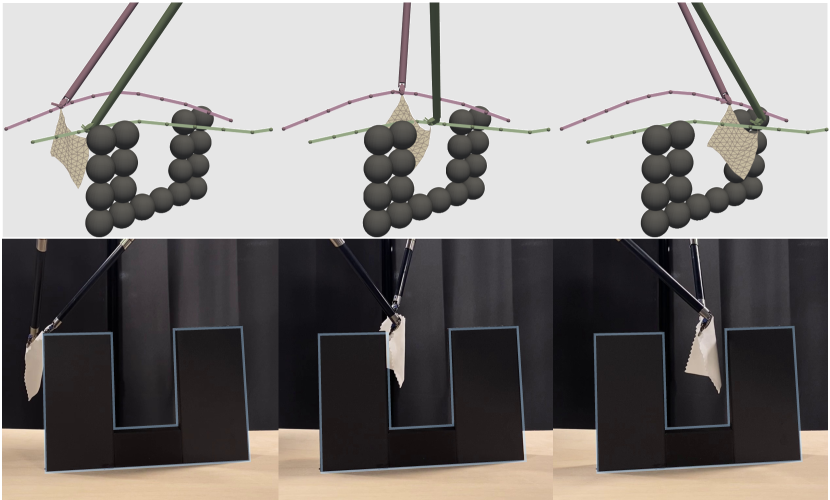
Figure 6: Visualizations of the trajectory in inverse kinematics simulation and on real robot. Two robot arms and corresponding control paths are colored by purple and green respectively. The obstacle in real experiment is highlighted in blue.

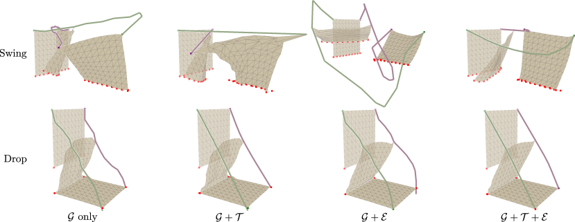
Figure 7: Visualizations of optimized cloth manipulation trajectories with different regularization strategies. The first row shows the results of the swing task. The second row shows the results of the drop task. For both tasks, from left to right we optimize for target loss $\mathcal{G}$ only, target loss $\mathcal{G}$ with trajectory regularization $\mathcal{T}$, target loss $\mathcal{G}$ with energy regularization $\mathcal{E}$ and target loss $\mathcal{G}$ with both regularization terms $\mathcal{T}$ and $\mathcal{E}$. Both $\mathcal{T}$ and $\mathcal{E}$ terms are crucial for finding an efficient and physics-aware control trajectory.

In Fig 6, we fed the trajectory into an inverse kinematics solver and let the dVRK robot follow the trajectory. It demonstrates that the trajectory is feasible for the real robot and satisfies the obstacle avoidance safety constraint. Due to the calibration accuracy, the real experiment does not recreate the control trajectory perfectly. We can mitigate the calibration error by adjusting the safety threshold to constrain the movement of the cloth. Furthermore, additional techniques (outside the scope of this paper) are available for addressing this calibration gap [13].

IV-C Ablation Study on Objective function

We conduct an ablation study on different forms of the proposed objective function. Specifically, we focus on different regularization terms’ impact on the quality of optimized trajectories. To facilitate this investigation, we simplify the trajectory optimization problem by isolating the influence of safety constraints, converting it into an unconstrained optimization problem. We introduce two supplemental cloth manipulation tasks for this study. They are (1) Swing: swinging the cloth and aligning the bottom edge of the cloth to a horizontal line; (2) Drop: dropping the cloth onto a flat surface and aligning its four corners to a flat square. We compare four variants of our objective, each minimizes:

1. $\mathcal{G}$ only: target error only.

2. $\mathcal{G}+\mathcal{T}$: target error and trajectory irregularity.

3. $\mathcal{G}+\mathcal{E}$: target error and potential energy.

4. $\mathcal{G}+\mathcal{T}+\mathcal{E}$: target error and both regularization terms.

Notice that the regularization terms $\mathcal{T}$ and $\mathcal{E}$ are scaled by $\alpha$ and $\beta$ respectively to control their influences. In the first task, we have $\alpha=1$ and $\beta=1e-5$. In the second task, we have $\alpha=1e-1$ and $\beta=1e-5$.

In Fig. 7, we show exemplar optimized cloth manipulation trajectories on two obstacle-free manipulation tasks. Even though all variants of our method successfully reach the target, different combinations of regularization terms yield significantly different trajectories and cloth dynamics. For $\mathcal{G}$ only, the cloth is moved to the target position but experiences a non-smooth trajectory and results in undesired wrinkles. Optimizing $\mathcal{G}+\mathcal{T}$ together, the trajectory converges to a smooth straight line. However, this ignores the dynamics of the cloth and causes extreme deformation. Conversely, when optimizing for $\mathcal{G}+\mathcal{E}$, the cloth exhibits less deformation overall, but the trajectory can become inefficient and irregular. The most favorable outcomes are generated when all three terms $\mathcal{G}+\mathcal{T}+\mathcal{E}$ are optimized simultaneously. Fig. 8 supports the same observation with quantitative data. As aforementioned, the target error (yellow) is always minimized to a sufficiently small value. However, by only optimizing $\mathcal{G}+\mathcal{T}$, the potential energy (purple) could still be large, which implies excessive deformation. Meanwhile, if we only optimize $\mathcal{G}+\mathcal{E}$, trajectory irregularity (red) is high, resulting in inefficient trajectories. It becomes evident that it is necessary to optimize all three terms $\mathcal{G}+\mathcal{T}+\mathcal{E}$ simultaneously to achieve an accurate, efficient, and physically plausible manipulation trajectory.

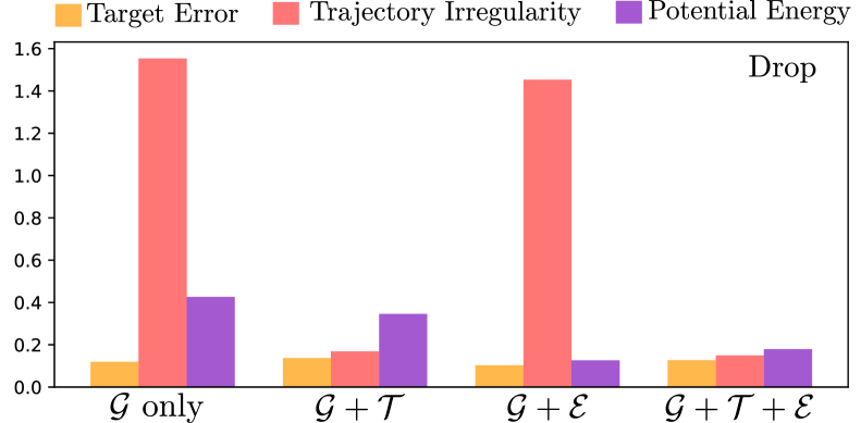
Figure 8: Comparison of target error, trajectory irregularity and potential energy across four variants of our method on the drop task. From left to right, we optimize for $\mathcal{G}$ only, $\mathcal{G}+\mathcal{T}$, $\mathcal{G}+\mathcal{E}$ and $\mathcal{G}+\mathcal{T}+\mathcal{E}$. All cost values are padded by $0.1$ so some small values are visible in the same chart.

V DISCUSSION & CONCLUSIONS

In this study, we introduce a cloth manipulation framework that places a strong emphasis on its awareness of cloth deformation physics and safety constraint satisfaction. Our framework leverages a differentiable XPBD simulation, which enables us to efficiently minimize the cost function with quasi-Newton optimization method to discover the optimal control sequence. We confirm that the proposed framework is able to yield safe, physics-aware manipulation trajectories through a series of safety constraints experiments and ablation studies. It holds the potential to advance robot autonomy in deformable object manipulation scenarios where safety and deformation mechanics are major concerns, such as autonomous surgery and elderly care.

References

- [1] Solvi Arnold, Daisuke Tanaka, and Kimitoshi Yamazaki. Cloth manipulation planning on basis of mesh representations with incomplete domain knowledge and voxel-to-mesh estimation. Frontiers in Neurorobotics, 16, 2023.
- [2] Xiao Ma, David Hsu, and Wee Sun Lee. Learning latent graph dynamics for visual manipulation of deformable objects. In 2022 International Conference on Robotics and Automation (ICRA), pages 8266–8273, 2022.
- [3] Wilson Yan, Ashwin Vangipuram, Pieter Abbeel, and Lerrel Pinto. Learning predictive representations for deformable objects using contrastive estimation. In Jens Kober, Fabio Ramos, and Claire Tomlin, editors, Proceedings of the 2020 Conference on Robot Learning, volume 155 of Proceedings of Machine Learning Research, pages 564–574. PMLR, 16–18 Nov 2021.
- [4] Júlia Borràs, Guillem Alenyà, and Carme Torras. A grasping-centered analysis for cloth manipulation. IEEE Transactions on Robotics, 36(3):924–936, 2020.
- [5] Kai Mo, Chongkun Xia, Xueqian Wang, Yuhong Deng, Xuehai Gao, and Bin Liang. Foldsformer: Learning sequential multi-step cloth manipulation with space-time attention. IEEE Robotics and Automation Letters, 8(2):760–767, 2023.
- [6] Siwei Chen, Xiao Ma, and Zhongwen Xu. Imitation learning as state matching via differentiable physics. In Proceedings of the IEEE/CVF Conference on Computer Vision and Pattern Recognition (CVPR), pages 7846–7855, June 2023.
- [7] Rishabh Jangir, Guillem Alenyà, and Carme Torras. Dynamic cloth manipulation with deep reinforcement learning. In 2020 IEEE International Conference on Robotics and Automation (ICRA), pages 4630–4636, 2020.
- [8] Jihong Zhu, Andrea Cherubini, Claire Dune, David Navarro-Alarcon, Farshid Alambeigi, Dmitry Berenson, Fanny Ficuciello, Kensuke Harada, Jens Kober, Xiang Li, Jia Pan, Wenzhen Yuan, and Michael Gienger. Challenges and outlook in robotic manipulation of deformable objects. IEEE Robotics & Automation Magazine, 29(3):67–77, 2022.
- [9] Hang Yin, Anastasia Varava, and Danica Kragic. Modeling, learning, perception, and control methods for deformable object manipulation. Science Robotics, 6(54):eabd8803, 2021.
- [10] Andreas Doumanoglou, Jan Stria, Georgia Peleka, Ioannis Mariolis, Vladimír Petrík, Andreas Kargakos, Libor Wagner, Václav Hlaváč, Tae-Kyun Kim, and Sotiris Malassiotis. Folding clothes autonomously: A complete pipeline. IEEE Transactions on Robotics, 32(6):1461–1478, 2016.
- [11] Jan Bender, Matthias Müller, and Miles Macklin. A survey on position based dynamics, 2017. In Proceedings of the European Association for Computer Graphics: Tutorials, EG ’17, Goslar, DEU, 2017. Eurographics Association.
- [12] Fei Liu, Entong Su, Jingpei Lu, Mingen Li, and Michael C. Yip. Robotic manipulation of deformable rope-like objects using differentiable compliant position-based dynamics. IEEE Robotics and Automation Letters, 8(7):3964–3971, 2023.
- [13] Fei Liu, Zihan Li, Yunhai Han, Jingpei Lu, Florian Richter, and Michael C. Yip. Real-to-sim registration of deformable soft tissue with position-based dynamics for surgical robot autonomy. In 2021 IEEE International Conference on Robotics and Automation (ICRA), pages 12328–12334, 2021.
- [14] Jingbin Huang, Fei Liu, Florian Richter, and Michael C. Yip. Model-predictive control of blood suction for surgical hemostasis using differentiable fluid simulations. In 2021 IEEE International Conference on Robotics and Automation (ICRA), pages 12380–12386, 2021.
- [15] Yunhai Han, Fei Liu, and Michael C. Yip. A 2d surgical simulation framework for tool-tissue interaction. CoRR, abs/2010.13936, 2020.
- [16] Miles Macklin, Matthias Müller, and Nuttapong Chentanez. Xpbd: position-based simulation of compliant constrained dynamics. In Proceedings of the 9th International Conference on Motion in Games, pages 49–54, 2016.
- [17] James Long, Katherine Burns, and Jingzhou (James) Yang. Cloth modeling and simulation: A literature survey. In Vincent G. Duffy, editor, Digital Human Modeling, pages 312–320, Berlin, Heidelberg, 2011. Springer Berlin Heidelberg.
- [18] Yunfei Bai, Wenhao Yu, and C. Karen Liu. Dexterous manipulation of cloth. Computer Graphics Forum, 35(2):523–532, 2016.
- [19] Dale McConachie, Andrew Dobson, Mengyao Ruan, and Dmitry Berenson. Manipulating deformable objects by interleaving prediction, planning, and control. The International Journal of Robotics Research, 39(8):957–982, 2020.
- [20] Cheng Chi, Benjamin Burchfiel, Eric Cousineau, Siyuan Feng, and Shuran Song. Iterative residual policy for goal-conditioned dynamic manipulation of deformable objects. In Proceedings of Robotics: Science and Systems (RSS), 2022.
- [21] Daniel Seita, Aditya Ganapathi, Ryan Hoque, Minho Hwang, Edward Cen, Ajay Kumar Tanwani, Ashwin Balakrishna, Brijen Thananjeyan, Jeffrey Ichnowski, Nawid Jamali, Katsu Yamane, Soshi Iba, John Canny, and Ken Goldberg. Deep imitation learning of sequential fabric smoothing from an algorithmic supervisor. In 2020 IEEE/RSJ International Conference on Intelligent Robots and Systems (IROS), pages 9651–9658, 2020.
- [22] Biao Jia, Zherong Pan, Zhe Hu, Jia Pan, and Dinesh Manocha. Cloth manipulation using random-forest-based imitation learning. IEEE Robotics and Automation Letters, 4(2):2086–2093, 2019.
- [23] Fan Zhang and Yiannis Demiris. Learning garment manipulation policies toward robot-assisted dressing. Science Robotics, 7(65):eabm6010, 2022.
- [24] Ravi P. Joshi, Nishanth Koganti, and Tomohiro Shibata. Robotic cloth manipulation for clothing assistance task using dynamic movement primitives. In Proceedings of the Advances in Robotics, AIR ’17, New York, NY, USA, 2017. Association for Computing Machinery.
- [25] Xingyu Lin, Yufei Wang, Jake Olkin, and David Held. Softgym: Benchmarking deep reinforcement learning for deformable object manipulation. In Conference on Robot Learning, 2020.
- [26] Yilin Wu, Wilson Yan, Thanard Kurutach, Lerrel Pinto, and Pieter Abbeel. Learning to manipulate deformable objects without demonstrations. In Proceedings of Robotics: Science and Systems (RSS), 07 2020.
- [27] Wei Xiao, Tsun-Hsuan Wang, Ramin Hasani, Makram Chahine, Alexander Amini, Xiao Li, and Daniela Rus. Barriernet: Differentiable control barrier functions for learning of safe robot control. IEEE Transactions on Robotics, 39(3):2289–2307, 2023.
- [28] Andrew Singletary, William Guffey, Tamas G. Molnar, Ryan Sinnet, and Aaron D. Ames. Safety-critical manipulation for collision-free food preparation. IEEE Robotics and Automation Letters, 7(4):10954–10961, 2022.
- [29] Li Wang, Aaron D. Ames, and Magnus Egerstedt. Safety barrier certificates for collisions-free multirobot systems. IEEE Transactions on Robotics, 33(3):661–674, 2017.
- [30] Octavio Villarreal, Victor Barasuol, Patrick M. Wensing, Darwin G. Caldwell, and Claudio Semini. Mpc-based controller with terrain insight for dynamic legged locomotion. In 2020 IEEE International Conference on Robotics and Automation (ICRA), pages 2436–2442, 2020.
- [31] Ruben Grandia, Andrew J. Taylor, Aaron D. Ames, and Marco Hutter. Multi-layered safety for legged robots via control barrier functions and model predictive control. In 2021 IEEE International Conference on Robotics and Automation (ICRA), pages 8352–8358, 2021.
- [32] Julian Nubert, Johannes Köhler, Vincent Berenz, Frank Allgöwer, and Sebastian Trimpe. Safe and fast tracking on a robot manipulator: Robust mpc and neural network control. IEEE Robotics and Automation Letters, 5(2):3050–3057, 2020.
- [33] Yilun Sun and Tim C. Lueth. Safe manipulation in robotic surgery using compliant constant-force mechanism. IEEE Transactions on Medical Robotics and Bionics, 5(3):486–495, 2023.
- [34] R. P. Joshi, N. Koganti, and T. Shibata. A framework for robotic clothing assistance by imitation learning. Advanced Robotics, 33(22):1156–1174, 2019.
- [35] Alexander Clegg, Wenhao Yu, Jie Tan, C. Karen Liu, and Greg Turk. Learning to dress: Synthesizing human dressing motion via deep reinforcement learning. ACM Trans. Graph., 37(6), dec 2018.
- [36] Mihai Dragusanu, Sara Marullo, Monica Malvezzi, Gabriele Maria Achilli, Maria Cristina Valigi, Domenico Prattichizzo, and Gionata Salvietti. The dressgripper: A collaborative gripper with electromagnetic fingertips for dressing assistance. IEEE Robotics and Automation Letters, 7(3):7479–7486, 2022.
- [37] P. Mitrano, D. McConachie, and D. Berenson. Learning where to trust unreliable models in an unstructured world for deformable object manipulation. Science Robotics, 6(54):eabd8170, 2021.
- [38] Zackory Erickson, Henry M. Clever, Greg Turk, C. Karen Liu, and Charles C. Kemp. Deep haptic model predictive control for robot-assisted dressing. In 2018 IEEE International Conference on Robotics and Automation (ICRA), pages 4437–4444, 2018.
- [39] Matthias Müller, Bruno Heidelberger, Marcus Hennix, and John Ratcliff. Position based dynamics. Journal of Visual Communication and Image Representation, 18(2):109–118, 2007.
- [40] Yuheng Zhi, Nikhil Das, and Michael Yip. Diffco: Autodifferentiable proxy collision detection with multiclass labels for safety-aware trajectory optimization. IEEE Transactions on Robotics, 38(5):2668–2685, 2022.
- [41] Pauli Virtanen, Ralf Gommers, Travis E. Oliphant, Matt Haberland, Tyler Reddy, David Cournapeau, Evgeni Burovski, Pearu Peterson, Warren Weckesser, Jonathan Bright, Stéfan J. van der Walt, Matthew Brett, Joshua Wilson, K. Jarrod Millman, Nikolay Mayorov, Andrew R. J. Nelson, Eric Jones, Robert Kern, Eric Larson, C J Carey, İlhan Polat, Yu Feng, Eric W. Moore, Jake VanderPlas, Denis Laxalde, Josef Perktold, Robert Cimrman, Ian Henriksen, E. A. Quintero, Charles R. Harris, Anne M. Archibald, Antônio H. Ribeiro, Fabian Pedregosa, Paul van Mulbregt, and SciPy 1.0 Contributors. SciPy 1.0: Fundamental Algorithms for Scientific Computing in Python. Nature Methods, 17:261–272, 2020.
- [42] Reuben Feinman. Pytorch-minimize: a library for numerical optimization with autograd, 2021.
- [43] Peter Kazanzides, Zihan Chen, Anton Deguet, Gregory S. Fischer, Russell H. Taylor, and Simon P. DiMaio. An open-source research kit for the da vinci® surgical system. In 2014 IEEE International Conference on Robotics and Automation (ICRA), pages 6434–6439, 2014.