Real-to-Sim Deformable Object Manipulation: Optimizing Physics Models with Residual Mappings for Robotic Surgery

Abstract

Accurate deformable object manipulation (DOM) is essential for achieving autonomy in robotic surgery, where soft tissues are being displaced, stretched, and dissected. Many DOM methods can be powered by simulation, which ensures realistic deformation by adhering to the governing physical constraints and allowing for model prediction and control. However, real soft objects in robotic surgery, such as membranes and soft tissues, have complex, anisotropic physical parameters that a simulation with simple initialization from cameras may not fully capture. To use the simulation techniques in real surgical tasks, the “real-to-sim” gap needs to be properly compensated. In this work, we propose an online, adaptive parameter tuning approach for simulation optimization that (1) bridges the real-to-sim gap between a physics simulation and observations obtained 3D perceptions through estimating a residual mapping and (2) optimizes its stiffness parameters online. Our method ensures a small residual gap between the simulation and observation and improves the simulation’s predictive capabilities. The effectiveness of the proposed mechanism is evaluated in the manipulation of both a thin-shell and volumetric tissue, representative of most tissue scenarios. This work contributes to the advancement of simulation-based deformable tissue manipulation and holds potential for improving surgical autonomy.

I INTRODUCTION

Handling deformable objects is a fundamental skill in robotic surgery, where surgeons precisely and minimally invasively treat soft tissue disease with robots. As the scope of robotic surgery expands, and as the gap between trained doctors and under-served patient populations widen, AI-driven surgical capabilities like autonomous suturing and tissue retraction become increasingly desirable and potentially necessary [1, 2]. Ultimately, these robots will require an understanding of tissue physics and deformable object manipulation in general in order to provide assistance or take over a surgical task.

Physics-based simulations have been proven to be a promising technique for deformable object manipulation (DOM) [3, 4, 5, 6]. It has been extensively researched from the modeling, motion planning, and data representations for perception perspectives [7]. The development of physical simulation environments can support a variety of deformable objects, including thin-shell fabric [8], linear elastic ropes [9], volumetric tissue [10, 11], and fluids [12].

Considering many existing deformable simulators, the high computational cost and “reality gap” are two factors that limit the conventional simulation approaches. These include Finite Element Methods (FEM) and mass-spring system [13]. Uncertainties, inaccurately calibrated parameters, and unmodeled physical effects can all lead to the gap between simulation and reality. As a result, many simulators need their parameters fine-tuned online in order to be deployable for real-world robotic tasks. With the intention of bridging the gap between reality and simulation, the phrase “real-to-sim” was first used in [10] to describe approaches that compensate for the simulated errors from live observations.

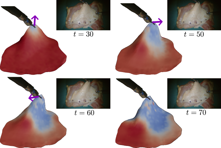
Figure 1: Our proposed online simulation parameter optimization method. It reveals suitable constraints’ stiffness parameters for a PBD simulation of a deformable tissue in an online manner. The tissue’s blue regions indicate lower stiffness, whereas red regions have higher stiffness. In this figure, the tissue is initialized with large stiffness parameters.

Our goal is to investigate the “real-to-sim” gaps by taking into account both known physical (geometric, mechanical) constraints describing tissue deformation and observable high-dimensional data, i.e., point cloud. For real-time applications such as surgical tissue manipulation, grasping, and retraction, it would also be necessary to identify the proper simulation parameters of soft bodies with a fast online simulation approach.

I-A Related Works

The “real-to-sim” problem has recently gained attention in the literature. Most of the existing works have been focusing on closing the gap through effective policy transfer in a reinforcement learning (RL) setup, as reviewed in [14, 15]. Most of these works only rely on simulating rigid objects in the scene and robots with kinematics [16, 17]. Recently, several papers used similar deep RL for deformable objects, such as cloth [18], tissue [19], and ropes [20]. However, these works don’t create explicit physical models but learn the system parameters or controls in an end-to-end manner. It leads to several typical problems with learning strategies, including generalizability and data-hunger.

Other methods rely on physics-based simulation to minimize the “real-to-sim” gap. Figure I presents a summary. In our previous paper [10], we directly update the simulated positions of the volumetric particles using the spatial gradient of the signed distance field of point cloud observation. However, the simulation parameters are not updated, necessitating frame-by-frame registration. Similarly, [21] optimizes for a simulation parameter, such as mass or stiffness, to minimize the difference between a simulation and the point cloud observation. Furthermore, the authors enhanced their approach in [22] as probabilistic inference over simulation parameters of the deformable object. However, their method is limited to thin-shell or linear objects (cloth, rope) with surface point clouds. Projective dynamics [23] were used to create a real-time physics-based model for tissue deformation, enhanced by a Kalman filter (KF) for refining the simulation with surface marker data. In a related work [24], they integrated FEM-based simulation into a deep reinforcement learning framework for grasping point policy learning, relying on offline stereo calibration for registration with the real world. For further improvements, [25] utilized a variational autoencoder with graph-neural networks to learn low-dimensional latent state variables’ probability distributions. These variables were iteratively updated using an ensemble smoother with data assimilation to align the simulation with real data. However, their offline training for specific FEM simulation datasets poses challenges in real-world applications, especially in surgery, where lengthy data-collection and pretraining phases are impractical.

TABLE I: summary of selected previous works that addressed deformable real-to-sim gap.

Methods Residual Parameters Update Object types [10] ✓ ✗ volumetric [21] ✗ ✓ thin-shell [25] ✓ ✗ volumetric Proposed ✓ ✓ both

I-B Contributions

In this work, we propose an online simulation parameter optimization framework for bridging the real-to-sim gap in deformable object manipulation. We believe it offers significant benefits in recovering a realistic physics simulation model for planning and control in DOM scenarios, including surgical autonomy. To this end, we present the following novel contributions:

• An online “real-to-sim” residual mapping module is seamlessly incorporated into a physics simulation loop to predicts a residual deformation $\Delta_{t}$ over time, which modifies simulation states to align with point cloud observations.

• The module estimates geometry-aware deformation for sub-surface simulation particles by considering geometric constraints. Therefore, it can be applied to thin-shell and volumetric deformable objects, covering wider surgical use cases than previous works.

• An online simulation optimization framework is used that adaptively updates stiffness parameters through loss functions that are informed by the residual mapping module, enhancing the simulation’s ability to predict future deformation and minimizing the the “real-to-sim” gap.

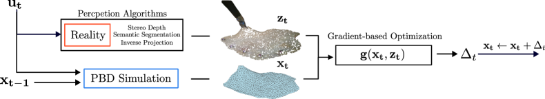
Figure 2: A flow chart of the proposed residual mapping module in the simulation loop. At each time step, a control $\mathbf{u_{t}}$ is applied to both the real tissue and the simulation. In response, the PBD simulation solves for $\mathbf{x_{t}}$. A perception pipeline processes imagery data to obtain a surface point cloud $\mathbf{z_{t}}$ of the tissue. The residual mapping module estimates the residual deformation $\Delta_{t}$ via optimization, which is then used to update the simulation state.

II METHOD

II-A Problem Formulation

Let the state of a soft body in a physics simulation at time stamps $t$ be $\mathbf{x_{t}}\in\mathbb{R}^{n\times 3}$, where $n$ is the number of particles of a mesh representing the soft body. We use the surface point cloud projected from the stereo-depth estimation as the observation, denoted as $\mathbf{z_{t}}\in\mathbb{R}^{m\times 3}$, where $m$ number of points in the point cloud observation. Let $\mathbf{u}_{t}$ be a point-based positional control that is applied to the real object and simulation simultaneously. In this work, we use an extended position-based dynamic (PBD) simulator, which formulates constraints with positional and geometric data. A constraints-based formulation of PBD is given as

$$\begin{split}\mathbf{x_{t}}=\mathcal{PBD}(\mathbf{x_{t-1}}&,\mathbf{u_{t}},\mathbf{\Gamma},\mathbf{C},\mathbf{k_{c}})\\ s.t.,\mathbf{C}(\mathbf{x_{t}})&=\mathbf{0},\ \mathbf{\Gamma}(\mathbf{x_{t}})=\mathbf{0}\\ \end{split}$$ (1)

where $\mathbf{\Gamma}$ are static (boundary) conditions that are enforced at each simulation step. The set of geometric constraints that define the deformation of across the simulation is $\mathbf{C}(\mathbf{x})=[C_{1}(\mathbf{x}),C_{2}(\mathbf{x}),\cdot\cdot\cdot,C_{I}(\mathbf{x})]^{\top}$. $\mathbf{k_{c}}\in\mathbb{R}^{I}$ is the set of weighting parameters associated with any kind of non-boundary constraint. One can interpret that $\{\mathbf{C,k_{c}}\}$ jointly defines the total energy potential (unitless) generated by constraints in a simulation:

$$\small\begin{split}\mathbf{U}(\mathbf{x})=\large\nicefrac{{1}}{{2}}\ \mathbf{C}(\mathbf{x})^{\top}\mathtt{diag}(\mathbf{k_{c}})\mathbf{C}(\mathbf{x})\end{split}$$ (2)

This is used by PBD to iteratively update particle positions, by minimizing this energy term:

$$\small\begin{split}\Delta\mathbf{x}&=\mathbf{M}^{-1}\nabla\mathbf{C}^{\top}\Delta\lambda\\ \Delta\mathbf{\lambda}&=-\Bigl{(}\nabla\mathbf{C}\mathbf{M}^{-1}\nabla^{\top}\mathbf{C}+\mathbf{\tilde{\alpha}}\Bigr{)}^{-1}\Bigl{(}\mathbf{C}+\mathbf{\tilde{\alpha}}\mathbf{\lambda}\Bigr{)}\\ \mathbf{\tilde{\alpha}}&=\mathtt{diag}(\mathbf{k_{c}})^{-1}/\Delta t^{2})\end{split}$$ (3)

in which $\mathbf{M}$ is a diagonal mass matrix and $\lambda$ is a Lagrange multiplier vector [26]. Note, while we demonstrate the proposed method with PBD simulation, it can be extended to real-to-sim problems in other differentiable simulators (e.g., FEM, projective dynamics [27]) without losing generality. We are only including the simulation step for PBD so one can follow the use of parameters through a forward simulation.

In this work, we aim at optimizing stiffness parameters associated with each particle, $\mathbf{k}\in\mathbb{R}^{n}$. This converts to elastic constraints’ weights in the simulation, denoted by $\mathbf{k_{d}}\subset\mathbf{k_{c}}$, by averaging stiffnesses across all involved particles. The value of $k_{d,i}\in\mathbf{k_{d}}$, that is, the weights of an elastic constraint $C_{i}(\mathbf{x})\in\mathbf{C}$, is

$$\small\begin{split}k_{d,i}=\Large\nicefrac{{1}}{{\mathtt{card}(Q_{i})}}\ \sum\nolimits_{q\in Q_{i}}k^{q},\ k^{q}\subset\mathbf{k}\end{split}$$

where particle indices $Q_{i}$ are considered by $C_{i}(\mathbf{x})$. Here, $Q_{i}$ contains $\mathtt{card}(Q_{i})$ number of particles that are connected via mesh edges, triangles, and tetrahedrons. This achieves non-homogeneous elastic stiffness across different regions of a soft body. Given that we generate a discretized mesh solely at the initial step, without engaging in any re-meshing procedures throughout the simulation, this imposes challenges on accurately representing isotropic material properties within the tissue. In light of this, we propose considering $\mathbf{k}$ as a spatially-variable stiffness.

We apply the developed framework on two types of deformable bodies: thin-shell objects that are simulated with a single layer of particles (similar to cloth) and volumetric objects that are simulated with tetrahedral meshes.

II-B Real-To-Sim Residual Mapping

We will learn a residual mapping module that is incorporated into the simulation loop to estimate the real-to-sim gap. This module will enable matching between simulation particles to a point cloud observation as shown in Figure 2. The method employs a gradient-based non-rigid point cloud registration to estimate the residual deformation $\Delta_{t}\in\mathbb{R}^{3\times n}$. To make the predicted residual mapping accurate and physically realistic, we consider both point cloud similarity and physical realness as cost functions to minimize.

Because the correspondence between the simulation particles and point cloud observation is unknown, we use Chamfer Distance as a measurement of similarities between two point clouds, which is computed by summing the squared distances between the nearest neighbor of two point clouds. For a thin-shell simulation, it is defined as

$$\small\begin{split}\mathcal{D}(\mathbf{x_{t}},\mathbf{z_{t}})&=\sum_{x\in\mathbf{x_{t}}}\min_{z\in\mathbf{z_{t}}}\|x-z\|^{2}_{2}+\sum_{z\in\mathbf{z_{t}}}\min_{x\in\mathbf{x_{t}}}\|z-x\|^{2}_{2}\\ \end{split}$$ (4)

A volumetric mesh can’t be directly aligned to a surface point cloud observation by minimizing Equation 4 as internal particles are not observed. Therefore, we alternatively minimize $\mathcal{D}(\mathbf{x^{\prime}_{t}},\mathbf{z_{t}})$ where $\mathbf{x^{\prime}_{t}}\in\mathbf{x_{t}}$ is the surface particles of the volumetric mesh, which is available from mesh initialization.

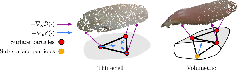
Figure 3: Visualizations of the proposed residual mapping module for thin-shell and volumetric objects. Purple and blue arrows represent deformation due to optimizing $\mathcal{D}(\cdot)$ and $\mathcal{E}(\cdot)$, respectively. For sub-surface particles that are unobservable to the camera, only $\mathcal{E}(\cdot)$ informs how it will deform.

We proposed an additional regularization term that is based on geometric constraints to inform the deformation of sub-surface particles of volumetric meshes. Meanwhile, this term is also essential to the physically realistic mapping of the thin-shell case. It is achieved by directly utilizing the geometric constraints that the PBD simulation defines in terms of the simulation’s energy potential:

$$\small\begin{split}\mathcal{E}(\mathbf{x_{t}})=\large\nicefrac{{1}}{{2}}\ \mathbf{C}(\mathbf{x_{t}})^{\top}\mathtt{diag}(\mathbf{k_{c}^{\prime}})\mathbf{C}(\mathbf{x_{t}})\end{split}$$ (5)

where $\mathbf{k_{c}^{\prime}}$ is an uniform user-defined weight matrix and $\mathbf{C}$ are PBD constraints. The overall idea is shown in Figure 3. Finally, a residual mapping function $\mathbf{g}(\mathbf{x_{t}},\mathbf{z_{t}})$ is defined as

$$\footnotesize\begin{split}\mathbf{g}(\cdot)=\begin{cases}\min_{\Delta_{t}}\mathcal{D}(\mathbf{x_{t}}+\Delta_{t},\mathbf{z_{t}})+\mathcal{E}(\mathbf{x_{t}}+\Delta_{t})&\ \ \textit{if thin-shell,}\\ \min_{\Delta_{t}}\mathcal{D}(\mathbf{x^{\prime}_{t}}+\Delta^{\prime}_{t},\mathbf{z_{t}})+\mathcal{E}(\mathbf{x_{t}}+\Delta_{t})&\ \ \textit{if volume.}\\ \end{cases}\end{split}$$ (6)

The above minimization problem is solved by performing 30 gradient descent steps with a learning rate of 50. At the end of a simulation step, $\Delta_{t}$ is used to update the current simulation state $\mathbf{x_{t}}$. Later, $\Delta_{t}$ is also viewed as a proxy to the real-to-sim gap that we seek to minimize through an online stiffness optimization approach.

II-C Online Stiffness Optimization

The proposed online optimization method differs from previous real-to-sim methods as it does not rely on training on previously collected trajectories. In this way, we are solving an online problem that is much more generalizable to real-world, unstructured environments. The algorithm is also embedded in the simulation loop as shown in Algorithm 1.

One term we want to minimize directly is the residual gap, which characterizes how much the simulation deviates from the observation for the current time step.

$$\begin{split}\mathcal{L}_{gap}=\|\mathbf{g}(\mathbf{x_{t}},\mathbf{z_{t}})\|\end{split}$$ (7)

Its partial derivative w.r.t stiffness parameters $\mathbf{k}$ is

$$\small\begin{split}\frac{\partial\mathcal{L}_{gap}}{\partial\mathbf{k}}&=\frac{\partial\|\mathbf{g}(\mathbf{x_{t}},\mathbf{z_{t}})\|}{\partial\mathbf{x_{t}}}\frac{\partial\mathcal{PBD}(\mathbf{x_{t-1}},...,\mathbf{k_{c}})}{\partial\mathbf{k_{c}}}\frac{\partial\mathbf{k_{c}}}{\partial\mathbf{k}}\end{split}$$

where the first term is available by differentiating through the residual mapping module, and the second term is obtained by differentiating through a simulation step in Equation 1.

The residual gap alone doesn’t consider historical information and, therefore, is sensitive to current observation noise. To address that, we introduce a history term computed over a set of previous time points $H_{t}$. It is defined as

$$\small\begin{split}\mathcal{L}_{hist}=\sum\nolimits_{h\in H_{t}}\|\mathbf{x}_{h}+\Delta_{h}-\mathcal{PBD}(\mathbf{x}_{h}+\Delta_{h},\mathbf{0},\mathbf{C},\mathbf{k_{c}})\|\end{split}$$ (8)

where $\mathbf{x}_{h}$ and $\Delta_{h}$ are snapshots of simulation states and residual mapping at time point $h$. Specifically, $H_{t}$ is constructed by uniformly sampling four snapshots from a window of the closest 20 previous frames. This loss function finds the stiffness parameters that keep each snapshot at rest when no control is provided (i.e., balancing external forces and internal elastic forces). This is a reasonable assumption when the system is not moving quickly.

1

Input : Predefined control sequence $\mathbf{U}$, stiffness $\mathbf{k}$, real tissue $R$, observation model $\mathcal{H}(R)$, residual mapping module $\mathbf{g}.$

2 $\mathbf{z_{0}}\leftarrow\mathcal{H}(R)$

// Initialize a mesh and constraints.

3 $\mathbf{x_{0}},\mathbf{C}\leftarrow\mathtt{initializeSimulation}(\mathbf{z_{0}})$

4$H_{t}\leftarrow[\ ]$

5for each $\mathbf{u_{t}}\in\mathbf{U}$ do

6       $R\leftarrow\textit{ApplyControl}(R,\mathbf{u_{t}})$

7      $\displaystyle\mathbf{x_{t}}\leftarrow\mathcal{PBD}(\mathbf{x_{t-1},u_{t},C,k_{c}})$

8      $\mathbf{z_{t}}\leftarrow\mathcal{H}(R)$

9      $\Delta_{t}\leftarrow\mathbf{g}(\mathbf{x_{t}},\mathbf{z_{t}})$

      // Compute $\mathcal{L}_{gap},\mathcal{L}_{hist},\mathcal{L}_{smooth}$

10       $\mathcal{L}_{total}\leftarrow\mathtt{computeLoss}(\Delta_{t},H_{t},\mathbf{k})$

11      $\displaystyle\mathbf{k}\leftarrow\mathtt{Optimize}(\mathbf{k},\nabla_{\mathbf{k}}\mathcal{L}_{total})$

12      $H_{t}\leftarrow[H_{t},\mathbf{x_{t}}+\Delta_{t}]$

13      $\mathbf{x_{t}}\leftarrow\mathbf{x_{t}}+\Delta_{t}$

14

Algorithm 1 Residual Mapping and Online Stiffness Optimization in a PBD simulation

In addition, we encourage a smooth spatial stiffness distribution by penalizing $\mathbf{k}$’s differences between neighboring particles. Let $F$ be a set of all faces or tetrahedrons that sorts tuples of particle indices, the smoothness loss is written as

$$\begin{split}\mathcal{L}_{smooth}=\frac{1}{2F}\sum_{f\in F}\sum_{i\in f}\sum_{j\in f}k_{i}-k_{j}\end{split}$$ (9)

where $k_{i}\in\mathbf{k}$ is the stiffness value of the i-th simulation particle. Note that intersection of different types of tissues is more complicated. which may be addressed by encouraging smoothness within individual semantic contours [28]. Lastly, all terms are summed up and back-propagated to the stiffness parameters. They are updated by taking a stochastic gradient descent step in every simulation step.

III EXPERIMENTS & RESULTS

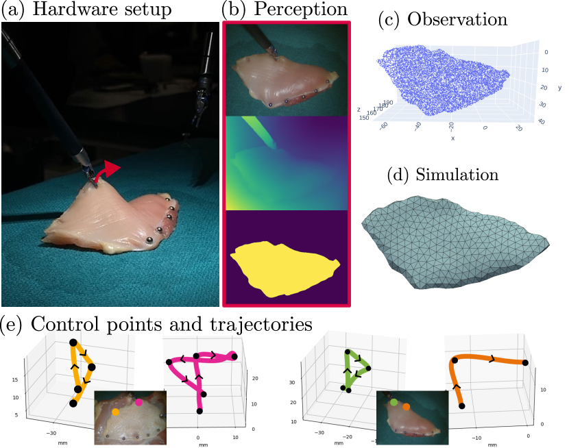
Figure 4: The real-to-sim experiment setup in this work. (a): a piece of chicken muscle manipulated by a dVRK manipulator. (b): A perception pipeline estimates depth and a semantic mask of the tissue. (c): surface point cloud is generated by a camera inverse projection. (d): A simulation mesh is created with the initial observation. (e): four manipulation trajectories are visualized with their starting point labeled on real images.

III-A Real Experiment Setup

The proposed real-to-sim framework is evaluated in two real-world deformable object manipulation examples of thin-shell and volumetric deformable tissues. Our experimental procedures involve the utilization of the da Vinci Research Kit (dVRK) [29], employing its robotic gripper to precisely manipulate soft tissue by executing predefined trajectories. Simultaneously, a stereo reconstruction pipeline processes stereo images captured by the da Vinci endoscopic camera in 720p, producing detailed tissue surface point clouds. Figure 4 shows our physical experiment setup. A piece of chicken skin and chicken muscle are used as subjects in our then-shell and volumetric experiments, respectively. They are roughly 3mm and 2 cm thick. In both experiments, we used metal pins to fix one side of the tissue onto the bottom plane.

Our perception pipeline comprises stereo-depth estimation, semantic segmentation, and inverse camera projection to generate surface point cloud observations of the soft tissues. We utilize the Raft-Stereo [30] for stereo disparity estimation. Segment-Anything [31] aids in identifying image pixels corresponding to the tissue, allowing us to extract the tissue’s surface point cloud from depth images. Subsequently, we employ inverse camera projection to convert the segmented depth into 3D positions. We also employ ArUco markers to determine the camera-to-world transformation. The point cloud is down-sampled to a size of 9000 points. Meshes are reconstructed by applying a ball-pivoting algorithm on the initial surface point cloud observation. For thin-shell tissues, we re-mesh them to have 600 particles. For volumetric experiments, we process the surface meshes by adding thickness using the solidify modifier in Blender. Then, we apply the same re-mesh operation followed by a tetrahedralization step. The simulation’s boundary conditions are selected at the locations of pins. The proposed residual mapping module requires a knowledge of surface particles. We manually selected them in this work. Note that it is also possible to select them automatically through visibility culling.

With the above setup, we collect in total four trajectories, two for thin-shell and two for volumetric experiments. From now, we refer to them as Thin-shell-1, Thin-shell-2, Volumetric-1, and Volumetric-2. The robotic gripper trajectories are manually labeled on the image.

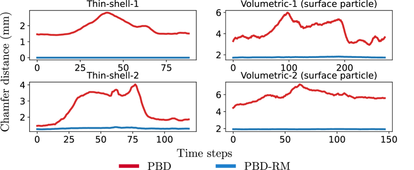
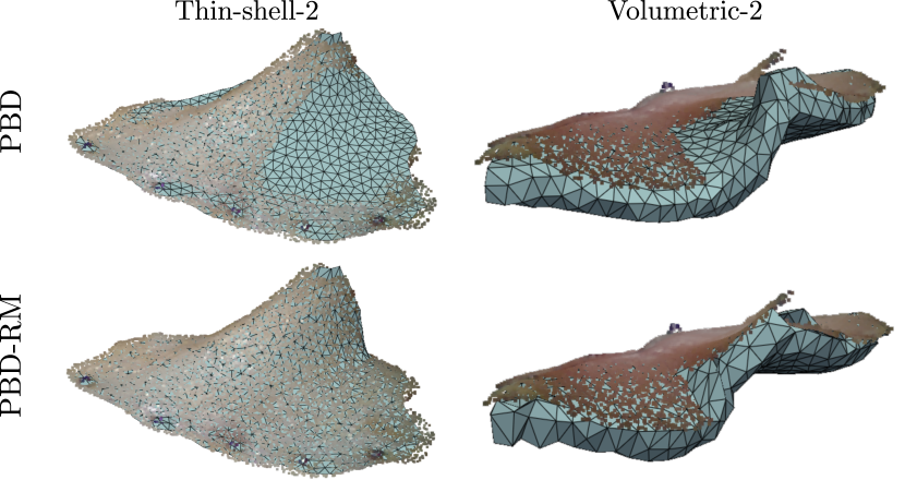
Figure 5: Comparison of the real-to-sim Chamfer distance (smoothed) between PBD and PBD-RM. In all four trajectories, the residual mapping module significantly reduces the Chamfer distance.

Figure 6: Surface point cloud observations overlaid on simulation meshes. With the residual mapping, the simulation mesh matches to textured point cloud observation better than the original PBD.

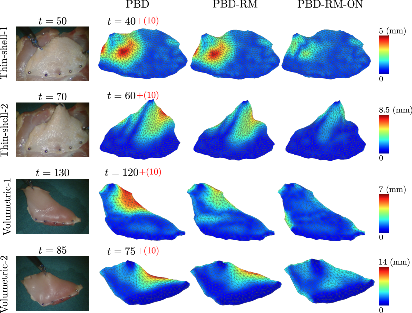
Figure 7: Average future gap of comparison methods over time (smoothed). Initialized with $\mathbf{k}^{2}$, both our proposed components, residual mapping and online stiffness optimization, show large error reduction over PBD.

Figure 8: Comparison of future gaps at selected time points. The gaps are visualized at $t=a+(b)$ time steps, meaning using the stiffness parameters at time $a$, forward the simulation for $b$ steps and then compute a gap. Both proposed PBD-RM and PBD-RM-ON can better predict the tissue’s future deformation behavior than the original PBD simulation.

III-B Implementation Details

This framework is implemented in Pytorch. Our PBD simulation adopts three types of geometric constraints: distance, volumetric, and shape-matching. They respectively preserve the distance between connected simulation particles, the volume of tetrahedral, and shapes formed by neighboring particles. We use distance and shape-matching constraints when simulating thin-shell tissue, whereas all three are used for volumetric tissue. Because we found that the effect of volumetric parameters is rather subtle, we assign a fixed value ${\footnotesize k_{vol}=1e10}$ and only optimize distance and shape-matching parameters. In addition, we observe that the value of stiffness parameters is only tangible in certain ranges, specifically with ${\footnotesize k_{dist}\in[0,10]}$ and ${\footnotesize k_{shape}\in[0,0.02]}$. Therefore, we force them to be in the above ranges with a sigmoid operation. As optimization-based methods are known to be sensitive to initialization, we evaluate the proposed method with three sets of initial parameters. They are ${\footnotesize\mathbf{k}^{1}:\{k_{dist}=5,k_{shape}=0.15\}}$, ${\footnotesize\mathbf{k}^{2}:\{k_{dist}=1,k_{shape}=0.1\}}$, ${\footnotesize\mathbf{k}^{3}:\{k_{dist}=0.2,k_{shape}=}$ ${\footnotesize{0.005}\}}$. All stiffness parameters are uniformly initialized. They are optimized with an Adam optimizer with a learning rate of 0.1. Later, we refer to a PBD simulation with a residual mapping module in its loop as PBD-RM and one that further performs online updates as PBD-RM-ON.

TABLE II: Comparison of time-average ($e_{t}$, $f_{t}$) of different methods with pre-defined initializations. Residual mapping (PBD-RM) and online optimization (PBD-RM-ON) improve prediction capabilities.

      Methods       $\mathbf{k}^{1}$       $\mathbf{k}^{2}$       $\mathbf{k}^{3}$       $\mathbf{k}^{1}$       $\mathbf{k}^{2}$       $\mathbf{k}^{3}$       Thin-shell-1       Thin-shell-2       PBD       $0.52,2.24$       $0.47,2.14$       $0.34,1.74$       $1.06,3.80$       $0.96,3.63$       $0.89,3.51$       PBD-DiffCloud       $0.45,\mathbf{1.76}$       $0.46,1.73$       $0.46,\mathbf{1.57}$       $0.90,4.22$       $0.97,4.14$       $1.02,4.28$       PBD-RM       $0.46,2.23$       $0.42,2.13$       $0.32,1.77$       $0.84,3.65$       $0.76,3.47$       $0.67,3.23$       PBD-RM-ON       $\mathbf{0.40},2.04$       $\mathbf{0.31,1.66}$       $\mathbf{0.30},1.72$       $\mathbf{0.65,2.98}$       $\mathbf{0.58,2.72}$       $\mathbf{0.62,2.89}$       PBD       $1.20,3.15$       $1.59,4.03$       $2.51,6.57$       $1.75,4.45$       $2.46,5.53$       $3.33,7.58$       PBD-RM       $1.02,3.06$       $1.13,3.52$       $1.30,4.32$       $14.1,4.33$       $1.65,5.00$       $1.86,5.70$       PBD-RM-ON       $\mathbf{0.94,2.91}$       $\mathbf{0.97,3.21}$       $\mathbf{1.00,3.38}$       $\mathbf{1.40,4.22}$       $\mathbf{1.48,4.56}$       $\mathbf{1.52,4.71}$

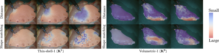
Figure 9: Projection of spatial distribution of optimized distance and shaping matching stiffness parameters over time. Red indicates a larger stiffness and blue indicates a smaller stiffness value. From left to right, stiffness distributions evolve over time.

III-C Residual Mapping Evaluation

In this section, we evaluate the effectiveness of applying the proposed residual mapping in the simulation loop. The simulations are initialized with stiffness $\mathbf{k_{C}}^{2}$. We measure the error between simulation and observation with Chamfer distances. Figure 6 shows that the errors are notably reduced in all trajectories using the proposed residual mapping module. They are stably kept at low levels throughout all trajectories. In the thin-shell cases, the proposed module shrinks the average errors from 1.84 mm and 2.55 mm to 0.001 mm and 1.31 mm. Likewise, the average errors are reduced from 4.24 mm and 5.79 mm to 1.78 mm and 1.93 mm in the volumetric case. Figure 6 visualizes the reduced differences between point clouds and mesh with our mapping module. For the volumetric case, the module simultaneously aligns the volumetric mesh’s surface particles to an observation and also deforms sub-surface particles, respecting PBD’s geometric constraints.

III-D Online Stiffness Optimization Evaluation

Here, we evaluate the method’s future deformation prediction capabilities. Specifically, we formulate an average future gap $e_{t}$ and a future keypoint error $f_{t}$ as our metrics. Knowing the current simulation state $\mathbf{x_{t}}$ and a future control sequence, we can roll out a simulation, without knowing future observations, to get future state sequence $[\mathbf{x_{t+1}}...\mathbf{x_{t+T}}]$. The average future gap is computed as

$$\small\begin{split}e_{t}&=\large\nicefrac{{1}}{{T}}\ \sum\nolimits_{s=1}^{T}\|\mathbf{g}(\mathbf{x_{t+s}},\mathbf{z}_{t+s})\|\\ \end{split}$$ (10)

Let $\mathbf{p}_{t}$ be a vector of keypoints’ positions at time $t$, and let $x^{i}_{t}$ represents the $i$-th particle in $\mathbf{x_{t}}$. The future keypoint error is defined as

$$\small\begin{split}f_{t}&=\sum_{p_{0},p_{t+T}\in\mathbf{p_{0}},\mathbf{p}_{t+T}}\|p_{t+T}-(\Delta p+p_{0})\|\\ \mathtt{where}\ \Delta p&\approx x^{nn}_{t+T}-x^{nn}_{0}\\ nn&=\mathtt{NearestNeighIndex}(\mathbf{x_{0}},p_{0})\\ \end{split}$$ (11)

Here, keypoint displacement $\Delta p$ is approximated by the displacement of $p$’s closest neighboring particles at $t=0$. For all experiments, we pick a future horizon $T=10$. A set of 15 keypoints are manually labeled on images every 10 frames for each trajectory.

For thin-shell experiments, we compare to DiffCloud [21], a baseline that optimizes simulation parameters by minimizing point cloud differences on a training trajectory. we it trained with the first 30 frames of each trajectory for 25 epochs. Table II shows a comparison on the two aforementioned metrics. Compared to the original PBD, PBD-RM shows reduced errors in all experiments, indicating that correcting the current simulation state with residual deformation leads to better future prediction. Compared to DiffCloud, PBD-RM-ON doesn’t consistently outperform it on the relatively shorter and simpler Thin-shell-1. However, it performs significantly better than all other methods in the other three experiments. DiffCloud produces unsatisfactory results on Thin-shell-2 as it overfits to the beginning of that trajectory, whereas the proposed method does not as it updates parameters online. Figure 8 supports the same observation, visualizing the average future gaps over time. Our PBD-RM-ON largely reduces the gap in the middle of trajectories where deformations are large. Figure 8 visualizes the spatial distribution of future gaps. It indicates larger errors located where tissues are experiencing bending. Both PBD-RM and PBD-RM-ON are effective at reducing errors in those regions. In Figure 9, the spatial distribution of optimized parameters is overlaid on real images. The stiffness parameters exhibit spatial and temporal variations. Effects such as distance stiffness lowering around the deforming areas in the thin-shell case can be attributed to the chicken skin’s inherent softness. In cases of heterogeneous parameter distributions, we hypothesize that their spatial variation may better approximate the complex behavior of the real tissue. Our future research will delve deeper into this effect.

IV Discussion & Conclusion

In this work, we have introduced an online simulation optimization framework designed to address the real-to-sim gap that arises in deformable tissue manipulation. A residual mapping module is seamlessly integrated into a simulation loop, achieving a minimal Chamfer distance between simulated particles and observation while preserving the geometric relationships in the simulator. Our optimization approach updates constraints’ stiffness parameters online. In real tissue experiments, it is proven to be effective at improving predictive performance. This improvement holds the potential for enhancing model-based control for DOM, such as identifying an accurate simulation model for model predictive control in autonomous surgeries. For deploying this work into real applications, one limitation is its computation speed. Currently, PBD-RM-ON takes 0.9s and 2.6s to complete a step for thin-shell and volumetric meshes. Despite that, it can be accelerated by GPU implementation or updating the parameters asynchronously. A possible future avenue of this work would be learning residual non-linear constraints to capture more intricate tissue behaviors.

References

- [1] Michael Yip, Septimiu Salcudean, Ken Goldberg, Kaspar Althoefer, Arianna Menciassi, Justin D. Opfermann, Axel Krieger, Krithika Swaminathan, Conor J. Walsh, He (Helen) Huang, and I-Chieh Lee. Artificial intelligence meets medical robotics. Science, 381(6654):141–146, 2023.
- [2] Aleks Attanasio, Bruno Scaglioni, Elena De Momi, Paolo Fiorini, and Pietro Valdastri. Autonomy in surgical robotics. Annual Review of Control, Robotics, and Autonomous Systems, 4(1):651–679, 2021.
- [3] Veronica E. Arriola-Rios, Puren Guler, Fanny Ficuciello, Danica Kragic, Bruno Siciliano, and Jeremy L. Wyatt. Modeling of deformable objects for robotic manipulation: A tutorial and review. Frontiers in Robotics and AI, 7, 2020.
- [4] Jihong Zhu, Andrea Cherubini, Claire Dune, David Navarro-Alarcon, Farshid Alambeigi, Dmitry Berenson, Fanny Ficuciello, Kensuke Harada, Jens Kober, Xiang Li, Jia Pan, Wenzhen Yuan, and Michael Gienger. Challenges and outlook in robotic manipulation of deformable objects. IEEE Robotics & Automation Magazine, 29(3):67–77, 2022.
- [5] Jinao Zhang, Yongmin Zhong, and Chengfan Gu. Deformable models for surgical simulation: A survey. IEEE Reviews in Biomedical Engineering, 11:143–164, 2018.
- [6] Jack Collins, Shelvin Chand, Anthony Vanderkop, and David Howard. A review of physics simulators for robotic applications. IEEE Access, 9:51416–51431, 2021.
- [7] Hang Yin, Anastasia Varava, and Danica Kragic. Modeling, learning, perception, and control methods for deformable object manipulation. Science Robotics, 6(54):eabd8803, 2021.
- [8] Qingyang Tan, Zherong Pan, Lin Gao, and Dinesh Manocha. Realtime simulation of thin-shell deformable materials using cnn-based mesh embedding. IEEE Robotics and Automation Letters, 5(2):2325–2332, 2020.
- [9] Fei Liu, Entong Su, Jingpei Lu, Mingen Li, and Michael C. Yip. Robotic manipulation of deformable rope-like objects using differentiable compliant position-based dynamics. IEEE Robotics and Automation Letters, 8(7):3964–3971, 2023.
- [10] Fei Liu, Zihan Li, Yunhai Han, Jingpei Lu, Florian Richter, and Michael C. Yip. Real-to-sim registration of deformable soft tissue with position-based dynamics for surgical robot autonomy. In 2021 IEEE International Conference on Robotics and Automation (ICRA), pages 12328–12334, 2021.
- [11] Yunhai Han, Fei Liu, and Michael C. Yip. A 2d surgical simulation framework for tool-tissue interaction. CoRR, abs/2010.13936, 2020.
- [12] Jingbin Huang, Fei Liu, Florian Richter, and Michael C. Yip. Model-predictive control of blood suction for surgical hemostasis using differentiable fluid simulations. In 2021 IEEE International Conference on Robotics and Automation (ICRA), pages 12380–12386, 2021.
- [13] François Faure, Christian Duriez, Hervé Delingette, Jérémie Allard, Benjamin Gilles, Stéphanie Marchesseau, Hugo Talbot, Hadrien Courtecuisse, Guillaume Bousquet, Igor Peterlik, and Stéphane Cotin. SOFA: A Multi-Model Framework for Interactive Physical Simulation, pages 283–321. Springer Berlin Heidelberg, Berlin, Heidelberg, 2012.
- [14] Wenshuai Zhao, Jorge Peña Queralta, and Tomi Westerlund. Sim-to-real transfer in deep reinforcement learning for robotics: a survey. In 2020 IEEE Symposium Series on Computational Intelligence (SSCI), pages 737–744, 2020.
- [15] Erica Salvato, Gianfranco Fenu, Eric Medvet, and Felice Andrea Pellegrino. Crossing the reality gap: A survey on sim-to-real transferability of robot controllers in reinforcement learning. IEEE Access, 9:153171–153187, 2021.
- [16] Yevgen Chebotar, Ankur Handa, Viktor Makoviychuk, Miles Macklin, Jan Issac, Nathan Ratliff, and Dieter Fox. Closing the sim-to-real loop: Adapting simulation randomization with real world experience. In 2019 International Conference on Robotics and Automation (ICRA), pages 8973–8979, 2019.
- [17] Xianzhi Li, Rui Cao, Yidan Feng, Kai Chen, Biqi Yang, Chi-Wing Fu, Yichuan Li, Qi Dou, Yun-Hui Liu, and Pheng-Ann Heng. A sim-to-real object recognition and localization framework for industrial robotic bin picking. IEEE Robotics and Automation Letters, 7(2):3961–3968, 2022.
- [18] Jan Matas, Stephen James, and Andrew J. Davison. Sim-to-real reinforcement learning for deformable object manipulation. In Aude Billard, Anca Dragan, Jan Peters, and Jun Morimoto, editors, Proceedings of The 2nd Conference on Robot Learning, volume 87 of Proceedings of Machine Learning Research, pages 734–743. PMLR, 29–31 Oct 2018.
- [19] Paul Maria Scheikl, Eleonora Tagliabue, Balázs Gyenes, Martin Wagner, Diego Dall’Alba, Paolo Fiorini, and Franziska Mathis-Ullrich. Sim-to-real transfer for visual reinforcement learning of deformable object manipulation for robot-assisted surgery. IEEE Robotics and Automation Letters, 8(2):560–567, 2023.
- [20] Yuqing Du, Olivia Watkins, Trevor Darrell, Pieter Abbeel, and Deepak Pathak. Auto-tuned sim-to-real transfer. In 2021 IEEE International Conference on Robotics and Automation (ICRA), pages 1290–1296, 2021.
- [21] Priya Sundaresan, Rika Antonova, and Jeannette Bohg. Diffcloud: Real-to-sim from point clouds with differentiable simulation and rendering of deformable objects, 2022.
- [22] Rika Antonova, Jingyun Yang, Priya Sundaresan, Dieter Fox, Fabio Ramos, and Jeannette Bohg. A bayesian treatment of real-to-sim for deformable object manipulation. IEEE Robotics and Automation Letters, 7(3):5819–5826, 2022.
- [23] Mehrnoosh Afshar, Jay Carriere, Hossein Rouhani, Tyler Meyer, Ron S. Sloboda, Siraj Husain, Nawaid Usmani, and Mahdi Tavakoli. Accurate tissue deformation modeling using a kalman filter and admm-based projective dynamics. IEEE/ASME Transactions on Mechatronics, 27(4):2194–2203, 2022.
- [24] Yafei Ou and Mahdi Tavakoli. Sim-to-real surgical robot learning and autonomous planning for internal tissue points manipulation using reinforcement learning. IEEE Robotics and Automation Letters, 8(5):2502–2509, 2023.
- [25] Mehrnoosh Afshar, Tyler Meyer, Ron S. Sloboda, Siraj Hussain, Nawaid Usmani, and Mahdi Tavakoli. Registration of deformed tissue: A gnn-vae approach with data assimilation for sim-to-real transfer. IEEE/ASME Transactions on Mechatronics, pages 1–9, 2023.
- [26] Miles Macklin, Matthias Müller, and Nuttapong Chentanez. Xpbd: position-based simulation of compliant constrained dynamics. In Proceedings of the 9th International Conference on Motion in Games, pages 49–54, 2016.
- [27] Tao Du, Kui Wu, Pingchuan Ma, Sebastien Wah, Andrew Spielberg, Daniela Rus, and Wojciech Matusik. Diffpd: Differentiable projective dynamics. ACM Trans. Graph., 41(2), nov 2021.
- [28] Shan Lin, Albert J. Miao, Jingpei Lu, Shunkai Yu, Zih-Yun Chiu, Florian Richter, and Michael C. Yip. Semantic-super: A semantic-aware surgical perception framework for endoscopic tissue identification, reconstruction, and tracking, 2023.
- [29] Peter Kazanzides, Zihan Chen, Anton Deguet, Gregory S. Fischer, Russell H. Taylor, and Simon P. DiMaio. An open-source research kit for the da vinci® surgical system. In 2014 IEEE International Conference on Robotics and Automation (ICRA), pages 6434–6439, 2014.
- [30] Lahav Lipson, Zachary Teed, and Jia Deng. Raft-stereo: Multilevel recurrent field transforms for stereo matching. In International Conference on 3D Vision (3DV), 2021.
- [31] Alexander Kirillov, Eric Mintun, Nikhila Ravi, Hanzi Mao, Chloe Rolland, Laura Gustafson, Tete Xiao, Spencer Whitehead, Alexander C. Berg, Wan-Yen Lo, Piotr Dollár, and Ross Girshick. Segment anything. arXiv:2304.02643, 2023.