AR-TTA: A Simple Method for Real-World Continual Test-Time Adaptation

Abstract

Test-time adaptation is a promising research direction that allows the source model to adapt itself to changes in data distribution without any supervision. Yet, current methods are usually evaluated on benchmarks that are only a simplification of real-world scenarios. Hence, we propose to validate test-time adaptation methods using the recently introduced datasets for autonomous driving, namely CLAD-C and SHIFT. We observe that current test-time adaptation methods struggle to effectively handle varying degrees of domain shift, often resulting in degraded performance that falls below that of the source model. We noticed that the root of the problem lies in the inability to preserve the knowledge of the source model and adapt to dynamically changing, temporally correlated data streams. Therefore, we enhance well-established self-training framework by incorporating a small memory buffer to increase model stability and at the same time perform dynamic adaptation based on the intensity of domain shift. The proposed method, named AR-TTA, outperforms existing approaches on both synthetic and more real-world benchmarks and shows robustness across a variety of TTA scenarios.

1 Introduction

Deep neural networks have been shown to achieve remarkable performance in various tasks. However, current machine learning models perform very well only when the test-time distribution is close to the training-time distribution. This poses a significant challenge since in a real-world application a domain shift can occur in many circumstances, e.g., weather change, time of day shift, or sensor degradation. For this reason, Test-Time Adaptation (TTA) methods have been widely developed in recent years [37, 35]. Their aim is to adapt the source data pre-trained model to the current data distribution on-the-fly during test-time, using an unlabeled stream of test data. Initial test-time adaptation methods considered a single domain shift at a time. To better simulate real-world challenges, a continual test-time adaptation [39] was recently proposed which involves constantly adapting the model to new domains, which is even more demanding.

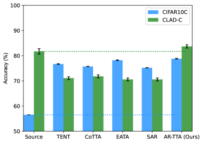
Figure 1: Continual test-time adaptation methods evaluated on synthetic (CIFAR-10C) and realistic (CLAD-C) domain shifts. Our method is the only one that consistently allows to improve over the naive strategy of using the (frozen) source model.

An efficient TTA method needs to work well in a wide range of settings. While some domain shifts occur abruptly, there are also several shifts that evolve gradually over time [20]. Additionally, the temporal correlation between consecutive frames violates the i.i.d. assumption. The model should be able to achieve stable performance when handling lengthy sequences, potentially extending indefinitely. Existing approaches are based on updating model parameters using calculated pseudo-labels or entropy regularization [39, 37]. Further, filtering of less reliable samples is often employed to reduce error accumulation and improve the computational efficiency [29, 30, 1]. However, all of the methods can become unstable due to the aforementioned factors, and as a result, the pseudo-labels become noisier and result in performance degradation [5]. Without using any source data the model is prone to catastrophic forgetting [28] of previously acquired knowledge.

Existing methods are mostly evaluated on synthetic datasets or on relatively short-length sequences [37, 39, 6] and as such it is not known how those methods will work in real-life scenarios. Therefore, we adapt the autonomous driving benchmark CLAD [36], to the continual adaptation setting. Moreover, we use a SHIFT dataset [34], which is synthetically generated but is very realistic, provides very long sequences, and allows us to specifically control for different factors (time of day, weather conditions).

In the proposed evaluation setup, we find out that current approaches lack the required stability, as their performance significantly deteriorates compared to the source model, see Figure 1. Additionally, we notice that they struggle to correctly estimate batch norm statistics with temporally correlated data streams and low batch sizes. In our method, we extend popular self-training framework [39, 37] with a small memory buffer, which is used during adaptation to prevent knowledge forgetting, without relying on heuristic-based strategies or resetting model weights that are often used [39, 30]. Thanks to using mixup data augmentation [40] relatively small number of samples are required. Furthermore, we develop a module for dynamic batch norm statistics adaptation, which interpolates the calculated statistics between those of pretrained model and those obtained during deployment, based on the intensity of domain shift. We call our method AR-TTA, as we improve Adaptation by using dynamic batch norm statistics and maintain knowledge by Repeating samples from the memory buffer combined with mixup data augmentation.

As a result, our proposed method AR-TTA is simple, stable, and works well across a range of datasets with different shift intensities, when using small batches of data and over very long sequences. Our main contributions can be summarized as follows:

• We evaluate and analyze current test-time adaptation methods on realistic, continual domain shift image classification data.

• We propose a simple continual TTA method based on dynamic batch normalization statistics update and a small memory buffer combined with mixup data augmentation.

• Extensive evaluation shows that the proposed method obtains state-of-the-art performance on multiple benchmarks with both artificial distortions and real-life ones from autonomous driving.

2 Related Work

Test-time adaptation (TTA). Domain adaptation methods can be split into different categories based on what information is assumed to be available during adaptation [38]. While in some scenarios, access to some labels in target distribution is available, the most common is unsupervised domain adaptation, which assumes that the model has access to labeled source data and unlabeled target data at adaptation time. Popular approaches are based on either minimizing the discrepancy between the source and target feature distributions [12, 17]. Alternative approaches are based on self-training, which uses the model’s predictions on the target domain as pseudo-labels to guide the model adaptation [42, 22].

Additionally, in test-time adaptation the model needs to adapt to the test-time distribution on the fly, in an online fashion. In the test-time training (TTT) method [35] the model solves self-supervised tasks on the incoming batches of data to update its parameters. TENT [37] updates only batch-norm statistics to minimize predictions entropy. This assumes that updating only batch norm statistics is sufficient to solve the problem, which might not be the case for real-world scenarios. EATA [29] further improves the efficiency of test-time adaptation methods, by using only diverse and reliable samples (with low prediction entropy). Additionally, it uses EWC [18] regularization to prevent drastic changes in parameters important for the source domain.

Contrary to the TENT and EATA approaches, CoTTA [39] updates the whole model. To prevent performance degradation it uses exponential weight averaging as well as stochastic model restoration, where randomly selected weights are reset to the source model. SAR [30] further improves by removing noisy test samples with large gradients and adding loss components that encourage model weights to go to a flat minimum. Nevertheless, they also use model reset, to prevent forgetting.

TTA benchmarks. The most popular setting for test-time adaptation includes using different classes of synthetic corruptions proposed in [14], which are then utilized for test-time adaptation, one at a time (so allowing model reset between different domains). However, in practical applications, the target distribution can easily change perpetually over time, e.g., due to changing weather and lightness conditions, or due to sensor corruptions, hence the setting of continual test-time adaptation was recently introduced [39]. The authors proposed to use a continual version of the corrupted benchmark (that is without model reset at domain boundaries).

Another popular dataset for continual test-time adaptation is DomainNet [31] which consists of images in different domains (e.g., sketches, infographics). Yet, the distribution shifts arising in the real world may be very different from the synthetic ones. Hence, recently a CLAD, autonomous driving benchmark [36] was introduced. It consists of naturally occurring distribution shifts like changes in weather and lighting conditions, traffic intensity, etc. It was developed for the supervised Continual Learning scenario. In this work, we use it for test-time adaptation, that is without using any label information. In our work, we also use SHIFT benchmark [34], a synthetically generated dataset for autonomous driving with realistic discrete and continuous shifts. Similarly to use, CoTTA [39] includes realistic domain shifts but their test is very small (1600 images). To sum up, we extend over previous TTA work by focusing on realistic continual domain shifts over very long sequences.

Continual Learning. Our work is also inspired by continual learning where the learner is presented with data from different tasks in a sequential fashion. Without access to the previous data from previous tasks, the model is prone to catastrophic forgetting [28]. Popular approaches use knowledge distillation to regularize changes in outputs of the model (compared to the model train on source task) [21] or regularize changes in model parameters [18]. On the other hand, exemplar-based approaches assume some limited access to the source data, which greatly helps to reduce the forgetting [27]. Further, some continual learning approaches focus on online setting, where each data point can be visited only once and small batch sizes are assumed [2].

3 Method

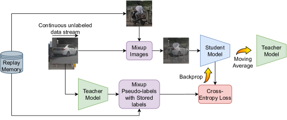
Figure 2: Our method AR-TTA adapts to the domain of an unlabeled continual stream of data utilizing exemplars of source pre-training data saved in the memory. We keep two identical neural network models with different sets of weights: the teacher model and the student model. We sample one exemplar from memory for each chosen image and mixup image pairs. Similarly, pseudo-labels from the teacher model are mixupped with the labels sampled from memory exemplars. The student model is updated based on cross-entropy loss between its predictions on augmented samples and augmented pseudo-labels. The teacher model is adapted based on an exponential moving average of student’s weights. Predictions for each image are taken from the teacher model.

The aim of TTA is to adapt the pre-trained model $f_{\theta_{0}}$ trained on the labeled source data $(\mathcal{X}^{S},\mathcal{Y}^{S})$ to the ever-changing stream of unlabeled test data batches $\textbf{x}^{T}$ on the fly during the evaluation.

Our proposed approach to TTA (AR-TTA) can be divided into three parts. We start the description by introducing the model update procedure in Subsection 3.1. Then, in Subsection 3.2 we explain the usage of experience replay with mixup augmentation. The process of adapting batch normalization statistics is presented in Subsection 3.3 The overview of our method is presented in Figure 2.

3.1 Weight-averaged Consistency

Updating the model’s weights during test-time is not a trivial task, considering the lack of data labels and the possibility of error accumulation due to noisy training feedback. Moreover, with the update procedure comes the stability-plasticity dilemma. The model should be stable enough to minimize the risk of deteriorating performance, model collapse, and catastrophic forgetting [11]. On the other hand, we want the model to be flexible to keep up with domain changes and adapt on time. Following previous works [9, 39], which show effective methods for alleviating mentioned challenges, we propose to employ self-training on pseudo-labels and keep two models, where one is updated by the exponential moving average of another’s weights.

We initialize two identical artificial neural network models, student model $f_{\theta}$ and teacher model $f_{\theta^{\prime}}$, with the identical weights obtained by training on source data. For each batch of test data $\textbf{x}_{t}^{T}$ at time step $t$ we generate predictions from both models. Teacher model predictions $\hat{y^{{}^{\prime}}}_{t}^{T}$ are used as soft pseudo-labels. The student model is updated by the cross-entropy loss between its predictions and the pseudo-labels:

$$\mathcal{L}_{\theta_{t}}(\textbf{x}_{t}^{T})=-\sum_{c}\hat{y^{{}^{\prime}}}_{t,c}^{T}\log\hat{y}_{t,c}^{T}$$ (1)

where $\hat{y}_{t,c}^{T}$ is the probability of class $c$ predicted by the student model.

Next, teacher’s weights $\theta^{{}^{\prime}}$ are updated by exponential moving average of student’s weights $\theta$:

$$\theta_{t+1}^{{}^{\prime}}=\alpha\theta_{t}^{{}^{\prime}}+(1-\alpha)\theta_{t+1}$$ (2)

where $\alpha$ is a smoothing factor.

As mentioned in  [39] using a weight-averaged teacher model ensures less noisy pseudo-labels since weight-averaged models over training steps often yield more accurate predictions than the final model and the added inertia prevents hasty, rapid weights update based on noisy self-training feedback. Moreover, susceptibility to catastrophic forgetting is decreased considering the fact that the weights are the combination of past iterations.

We do not limit the weights update only to affine parameters of batch normalization layers, as in many other TTA methods [29, 37, 30], and we update the whole model. We argue that adopting only batch normalization layers does not give the model enough flexibility to perform successfully on varying domains. We confirm this claim experimentally in the appendix and show that updating the whole models provides the best results, compared to fine-tuning only batch-norm layers or different blocks of the model.

The final predictions for the current test batch $\textbf{x}_{t}^{T}$ are the classes with the highest probabilities in pseudo-labels generated by the teacher model before the update.

3.2 Experience Replay with Adaptation

During continual test-time adaptation to unlabeled data, the model is exposed to training feedback that most likely differs from what it has learned during source pre-training. Pseudo-labels or entropy minimization feedback are not guaranteed to be accurate, and frequent model updates inevitably strive for significant error accumulation. These factors can be the cause of the model forgetting the initial knowledge. Noisy self-training and significant forgetting can even cause the model to collapse, as shown in [30]. For practical applications, a utilized method has to be reliable and the risk of collapsing has to be reduced to a minimum.

To alleviate this issue, we propose to use the class-balanced replay buffer of exemplars during adaptation to remind the model what it has learned and strengthen its initial knowledge. We take inspiration from continual learning approaches, which show that exemplars are one of the most effective approaches for this task [32, 4, 3, 36]. To fully take advantage of exemplars and make the latent representations of a model more robust for a given task, we follow a few of the continual learning works [24, 41] and propose to use Mixup data augmentation [40].

After completing the pre-training of the source model, we store a specific number of random exemplars from the labeled source data in the memory. The number of exemplars is the same for all classes. This works better than a random selection of exemplars, which we show in the appendix. In each test-time adaptation iteration, we randomly sample exemplars $\textbf{x}_{t}^{S}$, along with their labels $\textbf{y}_{t}^{S}$, from memory. The number of sampled exemplars is equal to the batch size. Mixupped batch of samples $\tilde{\textbf{x}}_{t}$ is generated by linearly interpolating samples from test data with samples from memory:

$$\tilde{\textbf{x}}_{t}=\lambda\textbf{x}_{t}^{T}+(1-\lambda)\textbf{x}_{t}^{S}$$ (3)

where $\lambda\sim$ Beta$(\psi,\rho)$, for $\psi,\rho\in(0,\infty)$. Similarly, labels for cross-entropy loss are the result of interpolation between pseudo-labels produced by the teacher model based on the current unmodified test batch $\hat{y}_{t}^{\prime T}$ and labels $\textbf{y}_{t}^{S}$ from the memory, with the same $\lambda$ parameter value:

$$\tilde{\textbf{y}}_{t}=\lambda\hat{\textbf{y}^{{}^{\prime}}}_{t}^{T}+(1-\lambda)\textbf{y}_{t}^{S}$$ (4)

Student model takes augmented batch $\tilde{\textbf{x}}_{t}$ as input. Its predictions are compared with interpolated labels $\tilde{\textbf{y}}_{t}$ to calculate the loss as described in the previous Subsection 3.1.

A similar approach to mixing exemplars from replay memory with the ones to train on was successfully used in LUMP [24], however, they used this method for the continual learning tasks.

Using experience replay along with the Mixup augmentation, helps the model preserve already obtained knowledge. Furthermore, having pseudo-labels mixed with certainly accurate labels for exemplars, makes the noisiness of pseudo-labels less impactful for the adaptation process.

3.3 Dynamic Batch Norm Statistics

Batch normalization [16] (BN) was created for reducing the internal covariate shift occurring during model training. It normalizes the distribution of a batch of input data utilizing the calculated running statistics, namely mean and variance, which is saved after the model training and used for the inference at test-time. While testing on out-of-distribution data, saved statistics are not correct and the normalization process fails to produce data with standard normal distribution which leads to poor model performance. Therefore, state-of-the-art test-time adaptation methods [39, 29, 37, 30] usually discard statistics calculated during training and estimate data distribution based on each batch of data separately. However, this way of estimating the statistics is flawed, since the sample size from data is usually too small to correctly estimate the data distribution, depending on batch size. Furthermore, samples might be temporally correlated (e.g. video input), which also is the cause of incorrect statistics estimates. In such cases, BN statistics from source data might be useful and closer to the actual data distribution, compared to the estimated values. To robustly estimate the correct normalization statistics we take the inspiration from [15] and propose to estimate BN statistics $\phi_{t}=(\mu_{t},\sigma_{t})$ at time step $t$ during test-time by linearly interpolating between saved statistics from source data $\phi^{S}$ and calculated values from current batch $\phi^{T}_{t}$:

$$\phi_{t}=(1-\beta_{ema})\phi^{S}+\beta_{ema}\phi^{T}_{t}$$ (5)

where $\beta_{ema}$ is a parameter that weights the influence of saved and currently calculated statistics.

Since the severity of distribution shift might vary, we need to adequately adjust the value of $\beta_{ema}$. It should be large in cases when the distribution shift is severe compared to the source domain and low when the distributions are similar. Following [15], we utilize the symmetric KL divergence as a measure of distance between distributions $D(\phi_{t-1},\phi_{t}^{T})$:

$$D(\phi_{t-1},\phi_{t}^{T})=\frac{1}{C}\sum_{i=1}^{C}KL(\phi_{t-1,i}||\phi_{t,i}^{T})+KL(\phi_{t,i}^{T}||\phi_{t-1,i})$$ (6)

The distance is used to calculate $\beta_{t}$ at time step $t$:

$$\beta_{t}=1-e^{-\gamma D(\phi_{t-1},\phi_{t}^{T})}$$ (7)

where $\gamma$ is a scale hyperparameter.

To compensate for the fact that the current distribution can be wrongly estimated and to provide more stability for the adaptation, we take into account previous $\beta_{1:t-1}$ values and use an exponential moving average for $\beta_{ema}$ update:

$$\beta_{ema}=(1-\alpha)\beta_{t-1}+\alpha\beta_{t}$$ (8)

where $\alpha$ is a hyperparameter.

The difference between our method and MECTA [15] is that we do not use the exponential moving average of calculated BN statistics, but instead, we keep the statistics from source data intact. We are motivated by the fact that changing this value cause the inevitable forgetting, accumulation of BN statistics estimate error, and susceptibility to temporal correlation. By keeping this value constant, we make sure that the estimation of the statistics on every batch does not cause the degradation of performance on domains similar to the source domain, leading to worse results than the frozen source model and abandonment of the legitimacy of using TTA methods. At the same time, we allow for a slight drift away from source data statistics, by using the exponential moving average of $\beta$ parameter, giving enough flexibility for the adaptation for severe domain shifts.

4 Experiments

Datasets and Benchmarks

We evaluate the methods on four image classification tasks: CIFAR10-to-CIFAR10C, ImageNet-to-ImageNet-C, CLAD-C continual learning benchmark [36] adapted to the test-time adaptation setting, and the benchmark created from the SHIFT dataset [34].

CIFAR10-to-CIFAR10C and ImageNet-to-ImageNet-C are widely used tasks in TTA. They involve training the source model on train split of clean CIFAR10/ImageNet datasets [19, 8] and test-time adaptation on CIFAR10C/ImageNet-C. CIFAR10C and ImageNet-C consist of images from clean datasets which were modified by 15 types of corruptions with 5 levels of severity[14]. They were first used for evaluating the robustness of neural network models and are now widely utilized for testing the adaptation capabilities of TTA methods. We test the adaptation on a standard sequence of the highest corruption severity level 5, frequently utilized by previous approaches [39, 29, 9]. For ImageNet-C we utilize a subset of 5000 samples for each corruption, based on RobustBench library [7], following [39].

CLAD-C [36] is an online classification benchmark for autonomous driving with the goal to introduce a more realistic testing bed for continual learning. Even though, to the best of our knowledge, it has not yet been used for testing TTA before, we chose this benchmark inspired by its realistic nature and the goal to simulate more real-world application setup. It consists of natural, temporal correlated, and continuous distribution shifts created by utilizing the data from SODA10M dataset [13]. The images taken at different locations, times of day, and weathers, are chronologically ordered, inducing distribution shifts in labels and domains. The classification task was created by cutting out the annotated 2D bounding boxes of six classes and using them as separate images for classification. Since it is designed for testing the continual learning setup and the model is originally supposed to be trained sequentially on the train sequences, we slightly modify the setup and pre-train the source model on the first train sequence. TTA is continually tested on the 5 remaining ones with the total number of 17092 images.

The SHIFT dataset is a synthetic autonomous driving dataset designed for continuous multi-task domain adaptation. It provides multiple types of data from the perspective of a car, including RGB images with various types of annotations. Images are taken in numerous types of realistic domains simulated in a virtual environment, including different weather and times of day. This dataset is not designed for a classification task. However, satisfied with the amount of data and the realism of the dataset, we decided to create the classification setup, using the same procedure as for the CLAD-C dataset, utilizing the 2D bounding box annotations. We train the source model on images taken at clean weather during the day and test the adaptation methods for various weather combinations and times of day. We end up with 14 different domains resulting in total of 380667 images. The high number of test samples provides a good simulation of what could happen during model deployment in a real world, ever-changing environment. We called our original continual test-time adaptation benchmark on SHIFT dataset SHIFT-C.

Methodology

Taking into account the realistic scenario, we examine the continual test-time adaptation setup where the model is continually adapted to new domains without any weight resetting to the source model state, unless it is a part of a tested method. To simulate the continuous stream of data and the need for the model to adapt quickly to the data it is provided with, we use a low batch size of 10. This is also the batch size commonly used in the online continual learning [25]. Considering a practical application on embedded device, low batch size could be also a result of limited computation resources and memory constraints, making it impossible to use higher batch sizes. We believe that it is important and more practical for TTA methods to be able to work on a reduced number of samples.

We primarily assess the methods using a straightforward mean classification accuracy metric. Additionally, to make every class equally important in class-imbalanced datasets, we use the average mean class accuracy (AMCA) metric. This metric calculates the mean accuracy over all classes, averaged for each domain.

The results are averaged between 3 random seeds. Samples from CIFAR10C and ImageNet-C are shuffled. Considering the sequential nature of data in CLAD-C and SHIFT-C benchmarks (video sequences), we did not want to shuffle images. Instead, to get seed-averaged results, we trained 3 source models with 3 different seeds and averaged the results between experiments with different models.

Baselines

To evaluate the performance of our method and validate its efficacy in handling realistic domain shifts, we conduct experiments involving five state-of-the-art methods as baselines: TENT-continual [37], EATA [29], CoTTA [39], and SAR [30]. Moreover, we show results for discarding BN statistics from source data and calculating the statistics for each batch separately (BN stats adapt) [33]. Additionally, we showcase the results obtained from the frozen source model to verify the effectiveness of adaptation (Source).

To provide a fair comparison with methods that do not require saving a small source data memory bank, we also show the results of our proposed method without the usage of replay memory. Furthermore, we show the results of baselines with a simple replay strategy method added in the appendix.

Implementation Details

Following other state-of-the-art TTA methods, we use pre-trained WideResnet28/ResNet50 models from RobustBench [7] model zoo for CIFAR10-to-CIFAR10C/ImageNet-to-ImageNet-C tasks. On the rest of the benchmarks, we utilize ResNet50 architecture with weights pre-trained on ImageNet obtained from torchvision library [26] and finetuned to the source data for the specific benchmark. Images from CLAD-C and SHIFT-C benchmarks are resized to 224x224 before being processed by the network. For our method, we use an SGD optimizer with a momentum equal to 0.9. The learning rate is set to 0.00025 for ImageNet-C and 0.001 for the rest of the benchmarks. The default replay memory size is 2000 samples, which is commonly used in continual learning settings [27] and adds only minor storage requirements. We provide experiments with different memory sizes in the appendix. The $\gamma$ value in Equation 7 is set to 10 for CIFAR10C and ImageNet-C, and 0.1 for CLAD-C and SHIFT-C. The $\alpha$ value for the exponential moving average of $\beta_{ema}$ in Equation 8 is set to 0.2. The initial $\beta_{ema}$ is equal to 0.1. The parameters $\psi$ and $\rho$ of the beta distribution, which are utilized to sample the interpolation parameter $\lambda$ for mixup augmentation (Equations 3, 4), are both set to a value of 0.4. We provide the results for different shapes of beta distribution in the appendix.

Since the batch size in our experiments is significantly lower than the ones used in the previous TTA works and we use two datasets on which the methods were not tested before, to allow for a fair comparison, we choose the learning rate for each method based on a grid search. The optimizers are chosen following the methods’ papers. For datasets that were not used in an EATA [29] paper, we also searched for the most optimal value of EATA’s method parameter $\epsilon$, which is responsible for filtering the redundant samples for model adaptation. The description and all the results of the parameter search can be found in the appendix. For the ease of prototyping and testing, we utilized the Avalanche library for continual learning [23].

4.1 Results

Artificial Domain Shifts

The results from CIFAR10-to-CIFAR10C and ImageNet-to-ImageNet-C tasks are shown in Tables 1 and 2. Artificial domain shifts pose a great challenge for source models, achieving only 56.5%/17.1% mean accuracy for CIFAR10C/ImageNet-C. Calculating BN statistics for each batch separately, already significantly improves the result to 75%/26.9% accuracy on corrupted images. Each of the compared state-of-the-art TTA methods uses the BN stats adapt technique, therefore their performance improves over it, but the increase in accuracy value is not that significant. EATA achieved the best mean accuracy of 78.2%/31.5% out of the tested state-of-the-art approaches. Our method AR-TTA outperforms all of the compared techniques achieving 78.8%/32.0% of mean accuracy. This shows the effectiveness of our method on standard continual TTA benchmarks.

Table 1: Classification accuracy (%) for the standard CIFAR10-to-CIFAR10C online continual test-time adaptation task.

	$t\xrightarrow{\hskip 398.33858pt}$
Method	Gaussian	shot	impulse	defocus	glass	motion	zoom	snow	frost	fog	brightness	contrast	elastic_trans	pixelate	jpeg	Mean
Source	27.7	34.3	27.1	53.1	45.7	65.2	58.0	74.9	58.7	74.0	90.7	53.3	73.4	41.6	69.7	56.5
BN stats adapt	67.3	69.4	59.7	82.7	60.4	81.4	83.0	78.1	77.7	80.6	87.3	83.4	71.4	75.3	67.9	75.0
TENT-continual [37]	67.9	71.4	62.5	83.2	62.9	82.1	83.8	79.5	79.7	81.4	87.8	84.3	73.5	78.2	71.6	76.7
EATA [29]	70.3	74.9	67.1	83.0	65.6	82.3	84.0	80.3	81.4	82.2	88.0	85.1	74.7	80.1	73.8	78.2
CoTTA [39]	72.5	76.4	70.5	80.6	66.6	78.3	80.1	75.8	77.0	77.1	83.8	77.3	72.0	75.5	72.2	75.7
SAR [30]	67.4	69.6	60.8	82.6	61.4	81.5	82.8	78.1	77.7	80.5	87.4	83.4	71.5	75.2	68.2	75.2
Ours (AR-TTA) w/o replay	69.5	73.6	63.3	83.5	63.0	82.5	84.5	80.2	80.4	81.9	88.4	83.8	74.2	76.9	74.5	77.3±0.07
Ours (AR-TTA)	69.2	74.8	66.4	84.5	67.8	83.7	85.2	81.4	82.7	83.4	88.0	84.7	73.9	78.6	77.0	78.8±0.13

Table 2: Classification accuracy (%) for the standard ImageNet-to-ImageNetC online continual test-time adaptation task.

Method	Mean
Source	18.1
BN stats adapt	26.9
TENT-continual [37]	29.2
EATA [29]	31.5
COTTA [39]	15.5
SAR [30]	30.8
Ours (AR-TTA) w/o replay	30.0±0.45
Ours (AR-TTA)	32.0±0.07

Natural Domain Shifts

Tests on natural domain shifts involve utilizing CLAD-C and SHIFT-C benchmarks. Results for CLAD-C are shown in Table 3. Calculating BN statistics for each batch does not improve the performance over the frozen source model and degrades the mean accuracy from 81.3% to 71.1%. Similarly, the state-of-the-art TTA methods achieve significantly lower mean accuracy, compared to the frozen source model, rendering them not effective for natural domain shifts. It suggests that benchmarking such methods on artificial domain shifts in form of corruptions is not a valuable estimate of the TTA method’s performance in practical applications. Moreover, it shows that estimating the BN statistics on each batch is not a trivial task, especially considering the temporal correlations in data. Keeping the pre-calculated statistics intact might sometimes be more beneficial for less severe domain shifts, on which the source model performs relatively well. Our method, which uses pre-calculated statistics and exemplars of source data during adaptation, outperformed state-of-the-art methods and achieves higher accuracy than the source model, which shows the effectiveness and adapting capabilities.

The close performance between the SAR and EATA methods, both achieving a mean accuracy of 71.1%, is attributed to the rigorous threshold-based sample filtering in both EATA and SAR. As a result of a coarse hyperparameter grid search (see the appendix), both methods tended to update on a very low number of samples in each parameter configuration. Moreover, SAR employs a model resetting scheme that frequently resets the weights of the model.

The mentioned techniques, although effective for the artificial CIFAR10C and ImageNet-C benchmarks, do not let both methods adapt well to CLAD-C and SHIFT-C test data.

Average mean class accuracy (AMCA) values show that the usage of replay memory might be crucial for high mean per-class accuracy.

Similar conclusions can be drawn from SHIFT-C benchmark results in Table 4. The frozen source model achieves impressive results, while state-of-the-art methods significantly degrade it. Moreover, the adaptation schemes of TENT and CoTTA methods caused the accuracy to be lower than the simple BN stats adaptation approach. Only AR-TTA was able to improve the source model performance during TTA.

Table 3: Classification accuracy and average mean class accuracy (AMCA) (%) for the CLAD-C continual test-time adaptation task.

	$t\xrightarrow{\hskip 85.35826pt}$
Method	T1	T2	T3	T4	T5	Mean day	Mean night	Mean	AMCA
Source	75.6	85.9	73.3	87.5	66.2	86.6	71.2	81.3	57.6
BN stats adapt	73.2	69.9	75.0	75.5	59.7	72.2	69.1	71.1	48.3
TENT-continual [37]	73.4	69.8	76.5	76.1	59.7	72.4	69.8	71.5	47.6
EATA [29]	73.3	69.9	75.0	75.6	59.7	72.2	69.1	71.1	48.4
CoTTA [39]	75.2	69.3	80.2	77.0	62.7	72.4	72.9	72.6	44.8
SAR [30]	73.2	69.9	75.0	75.5	59.7	72.2	69.1	71.1	48.3
Ours (AR-TTA) w/o replay	76.9	86.7	81.4	87.9	73.5	87.2	77.1	83.9±0.30	59.6±2.92
Ours (AR-TTA)	77.2	86.7	80.0	89.6	70.7	87.8	75.7	83.7±0.64	63.1±3.32

Table 4: Classification accuracy and average mean class accuracy (AMCA) (%) for the SHIFT-C continual test-time adaptation task.

	$t\xrightarrow{\hskip 398.33858pt}$
Method	daytime				dawn/dusk					night					Mean	AMCA
	cloudy	overcast	rainy	foggy	clear	cloudy	overcast	rainy	foggy	clear	cloudy	overcast	rainy	foggy
Source	97.9	98.2	97.5	92.5	93.6	94.1	94.0	93.5	91.5	89.1	89.3	90.6	89.1	90.7	93.5	89.5
BN stats adapt	89.1	88.9	88.0	86.2	85.3	84.8	87.3	83.5	84.8	81.3	81.2	80.3	79.6	83.5	85.1	69.9
TENT-continual [37]	89.6	88.8	87.5	84.6	83.3	81.2	85.0	80.7	80.2	78.0	77.0	76.1	75.7	77.6	82.7	57.6
EATA [29]	89.1	88.9	88.0	86.2	85.3	84.8	87.4	83.6	84.9	81.4	81.4	80.3	79.7	83.7	85.1	70.5
CoTTA [39]	88.2	87.1	84.1	80.5	78.7	76.2	80.5	74.0	74.9	71.5	70.3	67.3	64.9	66.2	77.4	47.2
SAR [30]	89.1	88.9	88.0	86.2	85.3	84.8	87.3	83.5	84.8	81.3	81.2	80.3	79.6	83.6	85.1	69.9
Ours (AR-TTA) w/o replay	96.4	96.5	95.3	93.2	92.2	91.9	93.2	91.4	91.8	88.7	88.7	88.6	87.5	91.2	92.4±0.25	83.5±0.96
Ours (AR-TTA)	97.7	98.0	97.4	94.3	94.2	95.5	94.8	95.2	93.1	92.3	92.7	93.0	91.4	92.6	94.8±0.03	90.2±0.24

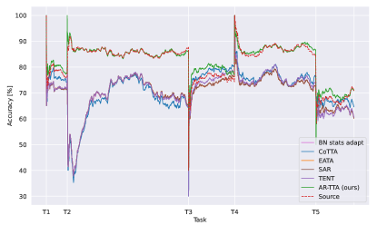
Figure 3: Batch-wise classification accuracy averaged in a window of 100 batches on CLAD-C benchmark for the chosen methods continually adapted to the sequences of data. The ticks on x-axis symbolize the beginning of next sequence and at the same time a different domain. Window for calculating average values is cleared in between sequences. Best viewed in color.

4.2 Ablation Study

Component Analysis

Table 5 shows the contribution of individual components used in the proposed method. For the initial setup A, we used a weight-averaged teacher model to generate pseudo-labels and cross-entropy loss to adapt the model of which the BN statistics from source data are discarded. Adding a simple replay method (B, E) by injecting randomly augmented exemplars from memory to the batch in a 1:1 ratio, did not improve the performance on every dataset. It can be seen that mixup data augmentation can boost the performance of a simple replay method (C). Moreover, dynamic BN statistics significantly contribute to the accuracy increase (D, E, AR-TTA), especially on the CLAD-C benchmark.

Table 5: Classification accuracy (%) for CIFAR10C and CLAD-C tasks for different configurations of the proposed method.

Method	CIFAR10C	CLAD-C
A: Weight-avg. teacher	75.7±0.07	71.1±0.53
B: A + Replay memory	77.3±0.16	69.0±0.66
C: B + Mixup	78.5±0.13	72.2±0.31
D: A + Dynamic BN stats	77.3±0.07	83.8±0.82
E: D + Replay memory	79.8±0.03	82.8±1.09
AR-TTA (Ours): E + Mixup	78.8±0.13	83.7±0.64

5 Conclusion

In this paper, we evaluate existing continual test-time adaptation (TTA) methods in real-life scenarios using more realistic data. Our findings reveal that current state-of-the-art methods are inadequate in such settings, as they fall short of achieving accuracies better than the frozen source model. This raises concerns about the applicability of certain TTA methods in real world and sheds light on the frequent model resets observed in some approaches. To address these limitations, we propose a novel and straightforward method called AR-TTA, based on the self-training framework. AR-TTA utilizes a small memory buffer of source data, combined with mixup data augmentation, and dynamically updates the batch norm statistics based on the intensity of domain shift.

Through experimental studies, we demonstrate that the AR-TTA method achieves state-of-the-art performance on various benchmarks. These benchmarks include realistic evaluations with small batch sizes, long test sequences, varying levels of domain shift, as well as artificial scenarios such as corrupted CIFAR10-C. Notably, AR-TTA consistently outperforms the source model, which serves as the ultimate baseline for feasible TTA methods. Our more realistic evaluation of TTA with a variety of different datasets provides a better understanding of their potential benefits and shortcomings.

Limitations The main limitation of our method is that we use a memory buffer from the source data, which might be an issue in resource-constrained scenarios or if there are some privacy concerns.

Impact Statement Test-time adaptation methods in machine learning might have a significant social impact. By improving accuracy, fairness, and robustness, these methods enhance the effectiveness of machine learning models in real-world applications. They contribute to reducing algorithmic bias, increasing equity, and promoting ethical considerations. However, responsible development and deployment are crucial to ensure positive outcomes and mitigate potential risks. Still, the problem of bias in the source dataset can influence the overall outcome.

Appendix

This document provides more results and describes our experimental procedure in detail. We attach the method code in the supplement. Additionally, the full codebase of the project will be open-sourced upon acceptance.

Appendix A Additional ablation study

A.1 Effect of replay memory size

The necessity to keep a set of samples from source data in memory can be problematic in memory-limited settings. We verified the possibility of minimizing the size of replay memory and evaluated our method with different numbers of stored samples. The results in Figure 4 show that our method is robust to replay memory size. There is no significant difference in accuracy between memory sizes of 500 and 10000 for both CIFAR10C and CLAD-C benchmarks. A slight degradation in performance can be seen with only 100 exemplars for CIFAR10C. Less severe domain shift in CLAD-C allows for a more significant reduction in the memory size without the performance drop.

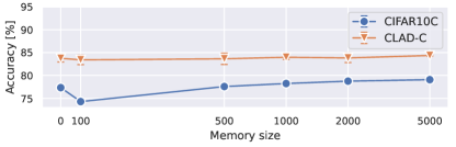
Figure 4: The influence of replay memory size on the resulting accuracy on CIFAR10C and CLAD-C benchmarks.

A.2 Baselines with simple replay memory

To ensure a fair comparison and check the state-of-the-art approaches’ performance with the use of replay memory, we added a simple replay method to each of them. A constant number of replay exemplars, equal to the batch size, was sampled on each batch from a class-balanced replay memory bank. The value of cross entropy loss calculated from exemplars was added to the original loss of each method. The results are in the Table 6. While the proposed method performs slightly worse than CoTTA on the CIFAR10C, it performs significantly better on the natural dataset. Most importantly, our method is the only one that constantly improves over the source model.

Table 6: Classification accuracy and average mean class accuracy (AMCA) (%) results for state-of-the-art methods with simple replay method added. The source method is a source model without adaptation.

Method	CIFAR10C	CLAD-C
	Mean	Mean	AMCA
Source	56.5	81.3	57.6
TENT-continual [37]	77.3	70.3	49.2
EATA [29]	78.6	71.1	48.4
CoTTA [39]	79.9	72.6	51.0
SAR [30]	75.3	71.1	48.3
AR-TTA (Ours)	78.8	83.7	63.1

A.3 Adapted weights

Table 7 shows the performance related to different configurations of adapted weights with our proposed method. We check the multiple configurations of adapting the last two layers, the first two layers, and only BN statistics. The best results are achieved by adapting the whole model.

Table 7: Classification accuracy (%) for different configurations of adapted weights with our proposed method AR-TTA.

CIFAR10C (WideResNet28)		CLAD-C (ResNet50)
Adapted weights	Mean	Adapted weights	Mean
block 1 (BN affine only)	61.4	layer 1 (BN affine only)	81.7
block 1, 2 (BN affine only)	26.3	layer 1, 2 (BN affine only)	81.5
block 2, 3 (BN affine only)	73.8	layer 3, 4 (BN affine only)	81.9
block 3 (BN affine only)	72.8	layer 4 (BN affine only)	82.1
block 1	17.4	layer 1	80.4
block 1, 2	13.9	layer 1, 2	81.6
block 2, 3	78.4	layer 3, 4	83.3
block 3	77.2	layer 4	82.8
BN affine only	75.1	BN affine only	81.8
Whole model (Ours)	78.8	Whole model (Ours)	83.7

A.4 Influence of beta distribution shape for mixup augmentation

The beta distribution in mixup augmentation is used to sample interpolation parameter between exemplars. Within our method, it controls the interpolation between test data samples and exemplars from the replay memory bank. By shaping this distribution we can adjust what are the fractions of replay and test data in the augmented samples. Results are shown in Table 8. The shape of the distribution did not have a significant impact on the results. The symmetric shape of the distribution, common for mixup augmentation, gives the best results.

Table 8: Classification accuracy (%) for CIFAR10C and CLAD-C tasks for different configurations of beta distribution parameters $\psi$ and $\rho$ for sampling interpolation parameter $\lambda\sim$ Beta$(\psi,\rho)$ required for mixup data augmentation.

$\psi$	$\rho$	CIFAR10C	CLAD-C
5.0	5.0	78.6	83.7
1.0	5.0	78.6	81.8
5.0	1.0	78.2	83.0
2.0	8.0	74.8	82.0
8.0	2.0	77.5	83.8
Ours
0.4	0.4	78.8	83.7

A.5 Additional component analysis

Table 9 shows results for different component configurations of our method. It includes the experiment without the usage of a weight-averaged teacher. We utilized pseudo-labels from the adapted model itself (configuration A). Additionally, we show the performance of our method when chosen exemplars for replay memory are not class-balanced.

Table 9: Classification accuracy (%) for CIFAR10C and CLAD-C tasks for different configurations of the proposed method.

Method	CIFAR10C	CLAD-C
A: Pseudo-labels	75.5±0.07	71.3±0.54
B: A + Weight-avg. teacher	75.7±0.07	71.1±0.53
C: B + Replay memory	77.3±0.16	69.0±0.66
D: C + Mixup	78.5±0.13	72.2±0.31
E: B + Dynamic BN stats	77.3±0.07	83.8±0.82
F: E + Replay memory	79.8±0.03	82.8±1.09
AR-TTA (Ours) with random memory selection	77.1±0.36	83.7±0.81
AR-TTA (Ours)	78.8±0.13	83.7±0.64

Appendix B Additional results

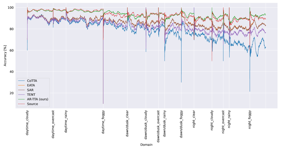
Figure 8: Batch-wise classification accuracy (%) averaged in a window of 500 batches on SHIFT-C benchmark for the chosen methods continually adapted to the sequences of data. The ticks on the x-axis symbolize the beginning of the next sequence and, at the same time, a different domain. The window to calculate the average values is cleared in between the sequences. Best viewed in color.

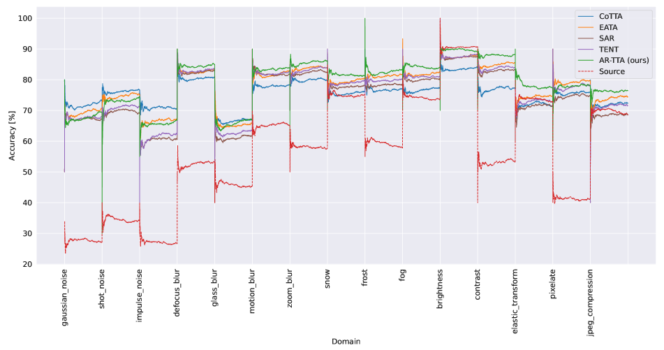
Figure 9: Batch-wise classification accuracy (%) averaged in a window of 500 batches on CIFAR10C benchmark for the chosen methods continually adapted to the sequences of data. The ticks on the x-axis symbolize the beginning of the next sequence and, at the same time, a different domain. The window to calculate the average values is cleared in between the sequences. Best viewed in color.

We present batch-wise accuracy plots for the CIFAR10C benchmark in Figure 9 and the SHIFT-C benchmark in Figure 8.

Appendix C Experimental details

We test the method in a continual manner on every benchmark, which means that the methods continually adapt the models without the reset to the source state in between the domains, unless it is a part of a tested method, as proposed in [39].

C.1 SHIFT-C benchmark details

The SHIFT-C benchmark is created using the SHIFT dataset [34]. The dataset consists of multiple types of autonomous driving data from the CARLA Simulator [10]. We used RGB images from the front view of a car, discrete domain shifts, and bounding box annotations. More specifically, we download the required data with the script from SHIFT’s website https://www.vis.xyz/shift/, using the following command:

⬇

python download.py –view ”front” \

–group ”[img, det_2d]” \

–split ”[train, val]” \

–framerate ”images” \

–shift ”discrete” TARGET_DIR

To load the data for experiments, we utilized shift-dev repository: https://github.com/SysCV/shift-dev.

Following the CLAD-C benchmark [36], we create an image classification task by cutting out the bounding box annotations and using each of them as a separate data sample. Bounding boxes with fewer than 1024 pixels are discarded. We pad the images by their shortest axis (modify the aspect ratio to 1:1) and resize them to 32x32. Bounding boxes in the dataset are categorized into six classes, and so are the created images. Example images are displayed in Figure 5. We present a class distribution in Figure 6.

We distinguish between domains by the course annotations of time of day and weather. The source model is trained on images from train split, taken at daytime in clear weather. The TTA is also tested on data from the train split, but from different weather conditions and times of the day. Details about the size of each domain can be found in Table 10.

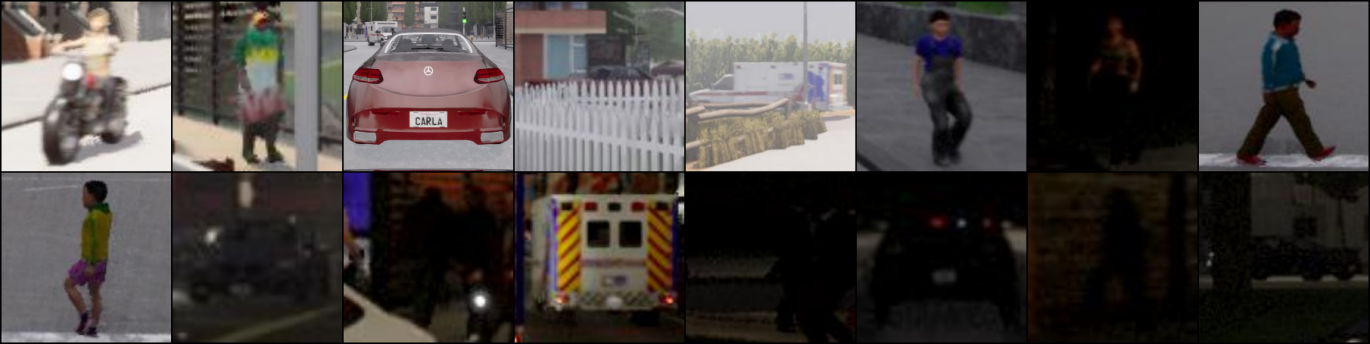
Figure 5: Example images sourced from various domains within the SHIFT-C benchmark.

Table 10: The number of samples in each domain in SHIFT-C benchmark

Domain nr	TIme of Day	Weather	Number of images
Source data	daytime	clean	57039
1		cloudy	41253
2		overcast	20497
3		rainy	59457
4		foggy	38590
5	dawn/dusk	clear	29543
6		cloudy	19985
7		overcast	9901
8		rainy	26677
9		foggy	20258
10	night	clear	28639
11		cloudy	18068
12		overcast	9471
13		rainy	32864
14		foggy	25464
Sum			437706

Figure 6: SHIFT-C benchmark class distribution.

C.2 Compared TTA methods implementation details

Implementations of the compared methods were taken from their official code repositories. We use all hyper-parameters and optimizers suggested by the papers or found in the code. We follow the standard model architectures used in TTA experiments and use WideResnet28 for CIFAR10C and ResNet50 for ImageNet-C, CLAD-C, and SHIFT-C. Moreover, since we use a smaller batch size (BS) of 10 and benchmarks that have not been used before in TTA, we search for the optimal learning rate (LR) for each method. We focus on lowering the LR, considering the decreased batch size. Additionally, we search for the $\epsilon$ hyperparameter of EATA to correctly reject samples for adaptation. The results of the parameter search can be found in Table 11. The details and parameters used for each method are described below.

TENT [37]

We use Adam optimizer with LR = 0.00003125 for every tested dataset. In the original paper, TENT uses LR = 0.001 for all the datasets except ImageNet, but it performed worse with this value in our setup.

CoTTA [39]

Adam optimizer with LR = 0.00025 is used for every tested benchmark, except ImageNet-C for which LR was equal to 0.00003125. The original implementation set LR to 0.001, but with an adjusted value, it achieved better results. We follow the suggestions for other hyperparameter values given by the authors. The restoration probability $p$ is set to 0.01, the smoothing factor of the exponential moving average of teacher weights $\alpha$ is equal to 0.999, and the confidence threshold for applying augmentations $p_{th}$ is set to 0.92.

EATA [29]

We use the SGD optimizer with a momentum of 0.9 and LR of 0.00025 for CIFAR10C, ImageNet-C, and CLAD-C. LR for SHIFT-C is equal to 0.00003125. The original EATA paper uses an LR value of 0.005/0.00025 for CIFAR10C/ImageNet-C, but they used BS = 64. After the search for the optimal $\epsilon$ parameter value for filtering redundant samples, we set it to 0.05/0.6 for CLAD-C/SHIFT. The value of $\epsilon$ for CIFAR10C/ImageNet-C is equal to 0.4/0.05, as in the original paper. The entropy constant $E_{0}$ is set to the standard value of 0.4$\times\ln C$, where $C$ was the number of classes, following the original paper and [30]. The trade-off parameter $\beta$ is equal to 1, and 2000 samples are used to calculate the fisher importance of model weights as for the CIFAR10 dataset in the original paper.

SAR [30]

SGD optimizer is used with the momentum of 0.9 and LR = 0.001 for CIFAR10C, and LR = 0.00025 for ImageNet-C, CLAD-C, and SHIFT-C. It almost aligns with the authors’ choice since, in original experiments, they used a learning rate equal to 0.00025/0.001 for ResNet/Vit models. The parameter $E_{0}$ is set to 0.4$\times\ln C$, as in the paper, similarly to EATA. We follow the authors’ choice of a constant reset threshold value $e_{0}$ of 0.2, and a moving average factor equal to 0.9. The radius parameter $\rho$ is set to the default value of 0.05.

AR-TTA (Ours)

We use SGD optimizer with momentum of 0.9. We set LR of 0.00025 for ImageNet-C, and 0.001 for the rest of benchmarks. The scale hyper-parameter $\gamma$ is set to 0.1 for CLAD-C and SHIFT-C, and 10 for ImageNet-C and CIFAR10C. $\alpha$ value for weighting the $\beta_{ema}$ is equal to 0.2. We set the initial $\beta_{ema}$ value to 0.1. The $\psi$ and $\rho$ parameters used for beta distribution to sample $\lambda$ for mixup is equal to the standard value of 0.4. We store 2000 of exemplars from source data for memory replay.

Table 11: Mean classification accuracy (%) for CIFAR10C, CLAD-C, and SHIFT-C continual test-time adaptation task for compared state-of-the-art methods with different learning rates and EATA’s $\epsilon$ parameter.

Method	learning rate	$\epsilon$	Mean CIFAR10C	Mean CLAD-C	Mean SHIFT-C	Mean ImageNet-C
CoTTA [39]	0.001	-	49.3	71.5	74.3	3.8
	0.00025	-	75.7	71.8	78.6	10.6
	0.00003125	-	74.5	71.8	76.2	15.3
TENT-continual [37]	0.001	-	24.3	64.4	63.4	0.6
	0.00025	-	72.3	71.0	75.3	3.1
	0.00003125	-	76.7	71.1	82.7	29.3
SAR [30]	0.001	-	75.2	70.6	86.0	11.3
	0.00025	-	75.1	70.6	86.0	31.5
	0.00003125	-	75.0	70.6	86.0	28.8
EATA [29]	0.001	0.60	-	70.1	80.4	-
	0.001	0.40	76.3	70.6	80.4	-
	0.001	0.10	-	70.6	86.0	-
	0.001	0.05	-	70.6	86.0	27.3
	0.00025	0.60	-	70.5	85.6	-
	0.00025	0.40	78.2	70.6	86.1	-
	0.00025	0.10	-	70.6	86.0	-
	0.00025	0.05	-	70.7	86.0	31.7
	0.00003125	0.60	-	70.6	86.1	-
	0.00003125	0.40	76.5	70.6	86.0	-
	0.00003125	0.10	-	70.6	86.0	-
	0.00003125	0.05	-	70.6	86.0	31.6

Appendix D AR-TTA method analysis

The $\gamma$ is a scale parameter of the distance between distributions $D(\phi_{t-1},\phi_{t}^{T})$. It determines the magnitude of the calculated values of $\beta$, which is used for linear interpolation between the saved source batch normalization (BN) statistics $\phi^{S}$ and the BN statistics calculated from the current batch $\phi_{t}^{T}$. The higher the value of $\gamma$, the higher the values of $\beta$ tend to be. At the same time, the higher the $\beta$ values, the more influence BN statistics from current batch have on interpolation and calculation of the finally used BN statistics. In Figure 7 we show the relationship between $\gamma$ parameter value and mean accuracy of our AR-TTA method for CIFAR10-to-CIFAR10C and CLAD-C benchmarks. We can see the contradicting trend between the two benchmarks. This suggests that the discrepancy in the data distribution between the source domain and the estimated distribution for each test data batch is more prominent in CIFAR10C compared to CLAD-C. This is in agreement with the results of the BN stats adapt [33] baseline method. BN stats adapt discards the BN statistics from the source data. Its performance was significantly better on CIFAR10C and worse on CLAD-C, compared to the fixed source model.

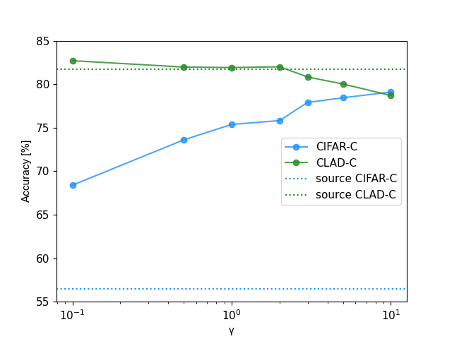
Figure 7: The relationship between mean classification accuracy (%) and the value of parameter $\gamma$ for CIFAR10C and CLAD-C benchmarks.

References

- [1] Motasem Alfarra, Hani Itani, Alejandro Pardo, Shyma Alhuwaider, Merey Ramazanova, Juan C Pérez, Zhipeng Cai, Matthias Müller, and Bernard Ghanem. Revisiting test time adaptation under online evaluation. arXiv preprint arXiv:2304.04795, 2023.
- [2] Rahaf Aljundi, Eugene Belilovsky, Tinne Tuytelaars, Laurent Charlin, Massimo Caccia, Min Lin, and Lucas Page-Caccia. Online continual learning with maximal interfered retrieval. In Advances in Neural Information Processing Systems 32: Annual Conference on Neural Information Processing Systems 2019, NeurIPS 2019, December 8-14, 2019, Vancouver, BC, Canada, pages 11849–11860, 2019.
- [3] M. Boschini, L. Bonicelli, P. Buzzega, A. Porrello, and S. Calderara. Class-incremental continual learning into the extended der-verse. IEEE Transactions on Pattern Analysis and Machine Intelligence, 45(05):5497–5512, may 2023.
- [4] Arslan Chaudhry, Albert Gordo, Puneet Kumar Dokania, Philip H. S. Torr, and David Lopez-Paz. Using hindsight to anchor past knowledge in continual learning. In AAAI Conference on Artificial Intelligence, 2019.
- [5] Chaoqi Chen, Weiping Xie, Wenbing Huang, Yu Rong, Xinghao Ding, Yue Huang, Tingyang Xu, and Junzhou Huang. Progressive feature alignment for unsupervised domain adaptation. In IEEE Conference on Computer Vision and Pattern Recognition, CVPR 2019, Long Beach, CA, USA, June 16-20, 2019, pages 627–636. Computer Vision Foundation / IEEE, 2019.
- [6] Dian Chen, Dequan Wang, Trevor Darrell, and Sayna Ebrahimi. Contrastive test-time adaptation. In IEEE/CVF Conference on Computer Vision and Pattern Recognition, CVPR 2022, New Orleans, LA, USA, June 18-24, 2022, pages 295–305. IEEE, 2022.
- [7] Francesco Croce, Maksym Andriushchenko, Vikash Sehwag, Edoardo Debenedetti, Nicolas Flammarion, Mung Chiang, Prateek Mittal, and Matthias Hein. Robustbench: a standardized adversarial robustness benchmark. arXiv preprint arXiv:2010.09670, 2020.
- [8] Jia Deng, Wei Dong, Richard Socher, Li-Jia Li, Kai Li, and Li Fei-Fei. Imagenet: A large-scale hierarchical image database. In 2009 IEEE conference on computer vision and pattern recognition, pages 248–255. Ieee, 2009.
- [9] Mario Döbler, Robert A. Marsden, and Bin Yang. Robust mean teacher for continual and gradual test-time adaptation. CoRR, abs/2211.13081, 2022.
- [10] Alexey Dosovitskiy, German Ros, Felipe Codevilla, Antonio Lopez, and Vladlen Koltun. CARLA: An open urban driving simulator. In Proceedings of the 1st Annual Conference on Robot Learning, pages 1–16, 2017.
- [11] Robert M. French. Catastrophic forgetting in connectionist networks. Trends in Cognitive Sciences, 3(4):128–135, 1999.
- [12] Yaroslav Ganin, Evgeniya Ustinova, Hana Ajakan, Pascal Germain, Hugo Larochelle, François Laviolette, Mario Marchand, and Victor S. Lempitsky. Domain-adversarial training of neural networks. In Gabriela Csurka, editor, Domain Adaptation in Computer Vision Applications, Advances in Computer Vision and Pattern Recognition, pages 189–209. Springer, 2017.
- [13] Jianhua Han, Xiwen Liang, Hang Xu, Kai Chen, Lanqing Hong, Jiageng Mao, Chaoqiang Ye, Wei Zhang, Zhenguo Li, Xiaodan Liang, and Chunjing Xu. Soda10m: A large-scale 2d self/semi-supervised object detection dataset for autonomous driving, 2021.
- [14] Dan Hendrycks and Thomas Dietterich. Benchmarking neural network robustness to common corruptions and perturbations. Proceedings of the International Conference on Learning Representations, 2019.
- [15] Junyuan Hong, Lingjuan Lyu, Jiayu Zhou, and Michael Spranger. Mecta: Memory-economic continual test-time adaptation. In ICLR, 2023.
- [16] Sergey Ioffe and Christian Szegedy. Batch normalization: Accelerating deep network training by reducing internal covariate shift. In Proceedings of the 32nd International Conference on International Conference on Machine Learning - Volume 37, ICML’15, page 448–456. JMLR.org, 2015.
- [17] Guoliang Kang, Lu Jiang, Yunchao Wei, Yi Yang, and Alexander Hauptmann. Contrastive adaptation network for single- and multi-source domain adaptation. IEEE Trans. Pattern Anal. Mach. Intell., 44(4):1793–1804, 2022.
- [18] James Kirkpatrick, Razvan Pascanu, Neil Rabinowitz, Joel Veness, Guillaume Desjardins, Andrei A Rusu, Kieran Milan, John Quan, Tiago Ramalho, Agnieszka Grabska-Barwinska, et al. Overcoming catastrophic forgetting in neural networks. Proceedings of the national academy of sciences, 114(13):3521–3526, 2017.
- [19] Alex Krizhevsky. Learning multiple layers of features from tiny images. pages 32–33, 2009.
- [20] Ananya Kumar, Tengyu Ma, and Percy Liang. Understanding self-training for gradual domain adaptation. In Proceedings of the 37th International Conference on Machine Learning, ICML 2020, 13-18 July 2020, Virtual Event, volume 119 of Proceedings of Machine Learning Research, pages 5468–5479. PMLR, 2020.
- [21] Zhizhong Li and Derek Hoiem. Learning without forgetting. In Computer Vision - ECCV 2016 - 14th European Conference, Amsterdam, The Netherlands, October 11-14, 2016, Proceedings, Part IV, volume 9908 of Lecture Notes in Computer Science, pages 614–629, 2016.
- [22] Hong Liu, Jianmin Wang, and Mingsheng Long. Cycle self-training for domain adaptation. In Marc’Aurelio Ranzato, Alina Beygelzimer, Yann N. Dauphin, Percy Liang, and Jennifer Wortman Vaughan, editors, Advances in Neural Information Processing Systems 34: Annual Conference on Neural Information Processing Systems 2021, NeurIPS 2021, December 6-14, 2021, virtual, pages 22968–22981, 2021.
- [23] Vincenzo Lomonaco, Lorenzo Pellegrini, Andrea Cossu, Antonio Carta, Gabriele Graffieti, Tyler L. Hayes, Matthias De Lange, Marc Masana, Jary Pomponi, Gido van de Ven, Martin Mundt, Qi She, Keiland Cooper, Jeremy Forest, Eden Belouadah, Simone Calderara, German I. Parisi, Fabio Cuzzolin, Andreas Tolias, Simone Scardapane, Luca Antiga, Subutai Amhad, Adrian Popescu, Christopher Kanan, Joost van de Weijer, Tinne Tuytelaars, Davide Bacciu, and Davide Maltoni. Avalanche: an end-to-end library for continual learning. In Proceedings of IEEE Conference on Computer Vision and Pattern Recognition, 2nd Continual Learning in Computer Vision Workshop, 2021.
- [24] Divyam Madaan, Jaehong Yoon, Yuanchun Li, Yunxin Liu, and Sung Ju Hwang. Representational continuity for unsupervised continual learning. In International Conference on Learning Representations, 2022.
- [25] Zheda Mai, Ruiwen Li, Jihwan Jeong, David Quispe, Hyunwoo Kim, and Scott Sanner. Online continual learning in image classification: An empirical survey. Neurocomputing, 469:28–51, 2022.
- [26] TorchVision maintainers and contributors. Torchvision: Pytorch’s computer vision library. https://github.com/pytorch/vision, 2016.
- [27] Marc Masana, Xialei Liu, Bartłomiej Twardowski, Mikel Menta, Andrew D Bagdanov, and Joost van de Weijer. Class-incremental learning: survey and performance evaluation on image classification. IEEE Transactions on Pattern Analysis and Machine Intelligence, 2022.
- [28] Michael McCloskey and Neal J Cohen. Catastrophic interference in connectionist networks: The sequential learning problem. In Psychology of learning and motivation, volume 24, pages 109–165. Elsevier, 1989.
- [29] Shuaicheng Niu, Jiaxiang Wu, Yifan Zhang, Yaofo Chen, Shijian Zheng, Peilin Zhao, and Mingkui Tan. Efficient test-time model adaptation without forgetting. In International Conference on Machine Learning, ICML 2022, 17-23 July 2022, Baltimore, Maryland, USA, volume 162 of Proceedings of Machine Learning Research, pages 16888–16905. PMLR, 2022.
- [30] Shuaicheng Niu, Jiaxiang Wu, Yifan Zhang, Zhiquan Wen, Yaofo Chen, Peilin Zhao, and Mingkui Tan. Towards stable test-time adaptation in dynamic wild world. In Internetional Conference on Learning Representations, 2023.
- [31] Xingchao Peng, Qinxun Bai, Xide Xia, Zijun Huang, Kate Saenko, and Bo Wang. Moment matching for multi-source domain adaptation. In Proceedings of the IEEE International Conference on Computer Vision, pages 1406–1415, 2019.
- [32] Sylvestre-Alvise Rebuffi, Alexander Kolesnikov, Georg Sperl, and Christoph H. Lampert. icarl: Incremental classifier and representation learning. In 2017 IEEE Conference on Computer Vision and Pattern Recognition (CVPR), pages 5533–5542, 2017.
- [33] Steffen Schneider, Evgenia Rusak, Luisa Eck, Oliver Bringmann, Wieland Brendel, and Matthias Bethge. Improving robustness against common corruptions by covariate shift adaptation. Advances in Neural Information Processing Systems, 33:11539–11551, 2020.
- [34] Tao Sun, Mattia Segu, Janis Postels, Yuxuan Wang, Luc Van Gool, Bernt Schiele, Federico Tombari, and Fisher Yu. SHIFT: a synthetic driving dataset for continuous multi-task domain adaptation. In Proceedings of the IEEE/CVF Conference on Computer Vision and Pattern Recognition (CVPR), pages 21371–21382, June 2022.
- [35] Yu Sun, Xiaolong Wang, Zhuang Liu, John Miller, Alexei A. Efros, and Moritz Hardt. Test-time training with self-supervision for generalization under distribution shifts. In Proceedings of the 37th International Conference on Machine Learning, ICML 2020, 13-18 July 2020, Virtual Event, volume 119 of Proceedings of Machine Learning Research, pages 9229–9248. PMLR, 2020.
- [36] Eli Verwimp, Kuo Yang, Sarah Parisot, Lanqing Hong, Steven McDonagh, Eduardo Pérez-Pellitero, Matthias De Lange, and Tinne Tuytelaars. Clad: A realistic continual learning benchmark for autonomous driving. Neural Networks, 161:659–669, 2023.
- [37] Dequan Wang, Evan Shelhamer, Shaoteng Liu, Bruno A. Olshausen, and Trevor Darrell. Tent: Fully test-time adaptation by entropy minimization. In 9th International Conference on Learning Representations, ICLR 2021, Virtual Event, Austria, May 3-7, 2021. OpenReview.net, 2021.
- [38] Mei Wang and Weihong Deng. Deep visual domain adaptation: A survey. Neurocomputing, 312:135–153, 2018.
- [39] Qin Wang, Olga Fink, Luc Van Gool, and Dengxin Dai. Continual test-time domain adaptation. In IEEE/CVF Conference on Computer Vision and Pattern Recognition, CVPR 2022, New Orleans, LA, USA, June 18-24, 2022, pages 7191–7201. IEEE, 2022.
- [40] Hongyi Zhang, Moustapha Cisse, Yann N. Dauphin, and David Lopez-Paz. mixup: Beyond empirical risk minimization. International Conference on Learning Representations, 2018.
- [41] Fei Zhu, Zhen Cheng, Xu-yao Zhang, and Cheng-lin Liu. Class-incremental learning via dual augmentation. In M. Ranzato, A. Beygelzimer, Y. Dauphin, P.S. Liang, and J. Wortman Vaughan, editors, Advances in Neural Information Processing Systems, volume 34, pages 14306–14318. Curran Associates, Inc., 2021.
- [42] Yang Zou, Zhiding Yu, Xiaofeng Liu, B. V. K. Vijaya Kumar, and Jinsong Wang. Confidence regularized self-training. In 2019 IEEE/CVF International Conference on Computer Vision, ICCV 2019, Seoul, Korea (South), October 27 - November 2, 2019, pages 5981–5990. IEEE, 2019.