Topological modes and spectral flows in inhomogeneous PT-symmetric continuous media

Abstract

In Hermitian continuous media, the spectral-flow index of topological edge modes is linked to the bulk topology via index theorem. However, most inhomogeneous continuous media in classical fluids and plasmas are non-Hermitian. We show that the connection between topological edge modes and bulk topology still exists in these non-Hermitian continuous media if the systems are PT-symmetric and asymptotically Hermitian. The theoretical framework developed is applied to the Hall magnetohydrodynamic model to identify a topological edge mode called topological Alfvén-sound wave in magnetized plasmas.

Introduction

Topological effects and classifications of electronic bands in crystal structures [1, 2, 3, 4, 5, 6, 7] have been studied extensively. Similar investigations have been carried out for photonic crystals [8, 9, 10] or phononic crystals [11, 12, 13, 14].

Recently, topological analysis has also found applications in classical continuous media [15, 16, 17, 18, 19, 20, 21, 22, 23, 24]. In continuous media without crystal structures, topological edge modes exist in the interface between two homogeneous bulk regions as shown in Fig. 1, akin to the situations in matters with crystal structures [1, 2, 3, 4, 5, 6, 7, 8, 9, 10, 11, 12, 13, 14]. However, there is a significant and fundamental difference. For the latter, topological edge modes are attributed to the topological differences between the eigenmode bundles over the two homogeneous bulk regions characterized by different Chern numbers. But for the former, both the eigenmode bundles over the two homogeneous bulk regions are topologically trivial, due to the fact that momentum space of continuous media are contractible [23]. In continuous media, there is no topological difference between homogeneous bulk regions. Instead, the topological physics manifests in the following manner. If an entire system, including both homogeneous and inhomogeneous regions, is Hermitian, then the spectral-flow index of the topological edge modes is identical to the index of the Weyl point (band crossing point) in the interface region by an Atiyah-Patodi-Singer (APS) [25] type of index theorem proved by Faure [26]. The index of the Weyl point is also known as the topological charge. In Ref. [27, 28], the Weyl point is referred to as Berry-Chern monopole. It was further emphasized that the Weyl point is necessarily in phase space and all eigenvector bundles over 2D surfaces in phase space surrounding the Weyl point are isomorphic and share the same Chern number that is defined to be the index of the Weyl point. [23].

Classical homogeneous media are Hermitian in general, but classical inhomogeneous media are mostly non-Hermitian. For example, a homogeneous fluid is Hermitian, whiles a fluid with flow shear is non-Hermitian which enables more interesting dynamical behaviors, such as the Kelvin-Helmholtz instability and turbulence. Nevertheless, classical inhomogeneous media, especially conservative systems, are often endowed with Parity-Time (PT) symmetries [29, 30, 31, 32] while being non-Hermitian. PT symmetry imposes structures while allowing complexity. Many well-known dynamics, such the Kelvin-Helmholtz instability [33, 34], the Rayleigh-Taylor instability [33], and the drift wave instability [35] are found to be governed by PT-symmetric systems and triggered by spontaneous PT-symmetry breaking.

Figure 1: Sketch of a 1D configuration in continuous media. $m(x)$ represent system parameters. $m(x)$ is constants in bulk 1 and 2, but varies smoothly from $m_{1}$ to $m_{2}$ in the interface.

We will take a theoretical abstraction and call an inhomogeneous non-Hermitian continuous system asymptotically Hermitian if its asymptotic Hamiltonian is Hermitian. Here, the asymptotic Hamiltonian is defined as the Hamiltonian when all spatial derivatives of the background system parameters are set to zero. In the present study, we will show that if an inhomogeneous continuous system is asymptotically Hermitian as well as PT-symmetric, and if the asymptotic Hamiltonian has a band gap near a Weyl point of two-fold degeneracy, then the non-Hermitian inhomogeneous system admits topological edge modes with real frequency in the neighborhood of the Weyl point. The spectral-flow index of the mode is identical to the topological charge of the Weyl point. We note that topological analysis of non-Hermitian systems have been reported in recent years [36, 37, 38, 39, 40, 41, 28], but the non-Hermitian continuous systems in the present study are qualitatively different because the non-Hermiticity is induced by inhomogeneity, which is the case in most classical fluids and plasmas.

The paper is organized as follows. We start from a family of simple two-band Hamiltonians to demonstrate the key physics of topological edge modes, spectrum flows, and topological charges in inhomogeneous continuous systems that are asymptotically Hermitian and PT-symmetric. The main result for general non-Hermitian inhomogeneous continuous systems is then established. In the last part, the general theoretical formalism developed is applied to identify a topological edge mode called topological Alfvén-sound wave (TASW) in the Hall magnetohydrodynamics (MHD) model for magnetized plasmas.

A two-band model

Consider the following two-band non-Hermitian Hamiltonians as simple examples of asymptotically Hermitian systems,

$$\mathcal{H}_{\epsilon}^{\alpha}[\lambda;x,\partial_{x}]=\begin{pmatrix}m(x)&\lambda-\partial_{x}\\ \lambda+\partial_{x}&-m(x)\end{pmatrix}+\mathrm{i}\epsilon m^{\prime}(x)\sigma^{\alpha}.$$ (1)

Here, $m(x)$ is a real function of $x$, representing a system parameter such as the mass term and $m^{\prime}\doteq\mathrm{d}m/\mathrm{d}x$. $\lambda$ is a constant system parameter, $\sigma^{\alpha}(\alpha=0,x,y,z)$ is an identity matrix or one of the Pauli matrices, and $\epsilon$ is a label indicating the order of the anti-Hermitian term. To study the possible topological modes of $\mathcal{H}_{\epsilon}^{\alpha}[\lambda;x,\partial_{x}]$, we need to investigate the corresponding symbol defined by the Wigner-Weyl transform $H_{\epsilon}^{\alpha}=\mathscr{W}(\mathcal{H}_{\epsilon}^{\alpha})$ [42, 43]. For the simple Hamiltonian in the form of Eq. (1), its symbol can be obtained by replacing $\hat{k}\doteq-\mathrm{i}\partial_{x}$ with $k$,

$$H_{\epsilon}^{\alpha}[\lambda;x,k]=\mathscr{W}(\mathcal{H}_{\epsilon}^{\alpha}){=}\begin{pmatrix}m&\lambda-\mathrm{i}k\\ \lambda+\mathrm{i}k&-m\end{pmatrix}+\mathrm{i}\epsilon m^{\prime}\sigma^{\alpha}.$$ (2)

The asymptotic Hamiltonian $H_{\epsilon}^{\alpha}$ is Hermitian with eigenvalues $\omega^{\pm}=\pm\sqrt{m^{2}+k^{2}+\lambda^{2}}$. Thus, there is a Weyl point (band crossing point) at $(m,k,\lambda)=(0,0,0)$, and its topological index can be easily calculated [27, 23, 26]. When $\epsilon>0$, $H_{\epsilon}^{\alpha}$ is non-Hermitian, and its eigenvalues are complex in general and support exceptional degeneracies [41].

The spectrum of $\mathcal{H}_{\epsilon}^{\alpha}[\lambda;x,\partial_{x}]$ is calculated in Appendix A. As expected for a non-Hermitian systems, when $\alpha\in\{0,x,z\}$ the spectrum is complex. We observe that $\mathcal{H}_{\epsilon}^{y}$ is an exception, which has a real spectrum for all $\epsilon\in\mathbb{R}$.

Here, we show why $\mathcal{H}_{\epsilon}^{y}$ is an exception from two perspectives. Firstly, $(\mathcal{H}_{\epsilon}^{y})^{*}=\mathcal{H}_{\epsilon}^{y}$, i.e., it is a real operator. Its anti-Hermitian part $\mathrm{i}\epsilon m^{\prime}(x)\sigma^{y}$ can be combined with the $\partial_{x}$ operator as a “covariant derivative” $(\partial_{x}-\epsilon m^{\prime})$. To calculate its spectrum, we perform a similarity transformation,

$$\mathcal{H}_{\epsilon}^{y}\to\mathcal{\widetilde{H}}_{\epsilon}^{y}=e^{-\epsilon m}\mathcal{H}_{\epsilon}^{y}e^{\epsilon m}=\mathcal{H}_{0}^{y}.$$ (3)

The non-Hermitian operator $\mathcal{H}_{\epsilon}^{y}$ has the same spectrum as the Hermitian operator $\mathcal{H}_{0}^{y}$. In particular, the $\mathcal{H}_{\epsilon}^{y}$ will have the same topological modes and spectral flows as $\mathcal{H}_{0}^{y},$ which is fully determined by its symbol $H_{0}^{y}=\mathscr{W}(\mathcal{H}_{0}^{y})$ according the index theorem by Faure [26].

Next, we interpret this result as a consequence of the non-Hermitian Hamiltonian being PT-symmetric. In the current context, time-reversal $\mathcal{T}$ is complex conjugation, and parity $\mathcal{P}$ is a $2\times 2$ constant unitary matrix

$$\mathcal{P}=\begin{pmatrix}P_{11}&P_{12}\\ P_{21}&P_{22}\end{pmatrix},$$ (4)

which satisfies $\mathcal{P}^{2}=1$ and $[\mathcal{P},\mathcal{T}]=0$. It is straightforward to verify that $\mathcal{H}_{\epsilon}^{y}$ is PT-symmetric with $\mathcal{P}=\sigma^{0}$, which implies that $\mathcal{H}_{\epsilon}^{y}$ can have real spectrum despite being non-Hermitian, when PT symmetry is not spontaneously broken. Since $\mathcal{H}_{\epsilon}^{y}$ is also asymptotically Hermitian, the domain of unbroken PT symmetry must contain a neighborhood of $\epsilon=0$. It turns out that this domain of unbroken PT symmetry includes all $\epsilon\in\mathbb{R}$, as implied by Eq. (3).

The important fact that $\mathcal{H}_{\epsilon}^{y}$ is similar to $\mathcal{H}_{0}^{y}$ for all $\epsilon\in\mathbb{R}$ can be generalized to the following class of generic two-band operators,

$$\mathcal{H}[\lambda;x,\partial_{x}]=\Big{[}\lambda{d}_{1\mu}+m{d}_{2\mu}-\mathrm{i}\partial_{x}{d}_{3\mu}+\mathrm{i}nd_{4\mu}\Big{]}{\sigma}^{\mu},$$ (5)

where $m(x)\,\text{and }n(x)$ are two real functions of $x$, $\sigma^{\mu}=(\sigma^{0},\bm{\sigma})$ is Pauli 4-vector, $d_{i\mu}$ are constant real 4-vectors. The Hamiltonian in Eq. (5) is assumed to be PT-symmetric for a properly chosen $\mathcal{P}.$ We prove that $\mathcal{H}[\lambda;x,\partial_{x}]$ is similar to a Hermitian operator.

The Hermitian part of its symbol $H_{\mathrm{H}}[\lambda;x,k]=[\lambda{d}_{1\mu}+m(x){d}_{2\mu}+k{d}_{3\mu}]{\sigma}^{\mu}$ supports a degeneracy point at $(\lambda,m,k)=(0,0,0)$. $\mathcal{H}$ being PT-symmetric means

$$(\mathcal{PT})\mathcal{H}(\mathcal{TP})=\mathcal{P}\mathcal{H}^{*}\mathcal{P}=\mathcal{H.}$$ (6)

Pick two orthonormal eigenvectors $\Psi_{i=1,2}$ of $\mathcal{PT}$ with eigenvalues $1$,

$$\mathcal{PT}\Psi_{i}=\mathcal{P}\Psi_{i}^{*}=\Psi_{i}.$$ (7)

Here, $\Psi_{i}$ are constant vectors. Let $\bm{\Psi}\doteq(\Psi_{1},\Psi_{2})^{\intercal}$ and it induces a similarity transformation for $\mathcal{H}$ ,

$$\mathcal{H}^{\prime}=\bm{\Psi}^{\dagger}\mathcal{H}\bm{\Psi}$$ (8)

Let $\bm{\Psi}^{\dagger}\sigma^{\mu}\bm{\Psi}=c_{\nu}^{\mu}\sigma^{\nu}$, we find $\mathcal{H}^{\prime}$ has the same form as Eq. (5) with $d_{i\mu}$ replaced by $\tilde{d}_{i\mu}\doteq c_{\mu}^{\nu}d_{i\nu}$. Since $\bm{\Psi}^{\dagger}\sigma^{\mu}\bm{\Psi}$ is Hermitian, $c_{\nu}^{\mu}$ must be real, so are $\tilde{d}_{i\mu}$.

From Eq. (6), we have

$$(\mathcal{H}_{ij}^{\prime})^{*} =(\Psi_{i}^{*})^{\dagger}\mathcal{H}^{*}\Psi_{j}^{*}=(\mathcal{P}\Psi_{i})^{\dagger}(\mathcal{P}\mathcal{H}\mathcal{P})(\mathcal{P}\Psi_{j})$$ (9)

$$=\Psi_{i}^{\dagger}\mathcal{P}^{\dagger}\mathcal{P}\mathcal{H}\mathcal{P}^{\dagger}\mathcal{P}\Psi_{j}=\mathcal{H}_{ij}^{\prime},$$

which means that $\mathcal{H}^{\prime}$ is a real operator. Thus, the coefficients in front of $\sigma_{y}$ must be imaginary, and the coefficients of $\sigma_{0},\sigma_{x},\sigma_{z}$ must be real. So $\mathcal{H}^{\prime}$ has the following form,

$$\mathcal{H}^{\prime}=\sum_{\mu}^{0,x,z}\Big{[}\lambda\tilde{d}_{1\mu}+m\tilde{d}_{2\mu}\Big{]}{\sigma}^{\mu}+\mathrm{i}\Big{[}n\tilde{d}_{4y}-\partial_{x}\tilde{d}_{3y}\Big{]}{\sigma}^{y}.$$ (10)

Let $\gamma\doteq\int n(x)\mathrm{d}x$. The anti-Hermitian part of $\mathcal{H}^{\prime}$ can be transformed away by a similarity transform,

$$\mathcal{H}^{\prime\prime}=\mathrm{e}^{-\gamma}\mathcal{H}^{\prime}\mathrm{e}^{\gamma}=\sum_{\mu}^{0,x,z}\Big{[}\lambda\tilde{d}_{1\mu}+m\tilde{d}_{2\mu}\Big{]}{\sigma}^{\mu}-\mathrm{i}\partial_{x}\tilde{d}_{3y}{\sigma}^{y}.$$ (11)

The spectrum of the PT-symmetric $\mathcal{H}$ in Eq. (5) is identical to that of the Hermitian operator $\mathcal{H}^{\prime\prime}$. In particular, $\mathcal{H}$ admits topological edge modes whose spectral-flow index is determined by the symbol $H^{\prime\prime}=\mathscr{W}(\mathcal{H}^{\prime\prime})$ according to Faure’s index theorem [26].

Inhomogeneous PT-symmetric continuous media

We now further generalize the result by showing that when an inhomogeneous medium is asymptotically Hermitian and PT-symmetric, it can be approximated by a two-band Hamiltonian of the form of Eq. (5) near the Weyl point of two-fold degeneracy of the asymptotic Hamiltonian symbol. Consider a 1D continuous media with $N$ field variables. The dynamics of the system is governed by a asymptotically Hermitian, PT-symmetric Hamiltonian operator $\mathcal{H}[\lambda;x,\partial_{x}]$, which depends on coordinate $x$ through a system parameter $m(x)$ and its derivatives. Here, we make a technical assumption that the inhomogeneity experienced by the edge mode is weak, i.e., $\epsilon\doteq\delta/l\ll 1$, where $\delta$ is the scale length of the edge mode and $l$ that of $m(x)$. In dimensionless variable, it implies that the $i$-th order derivatives $m^{(i)}$ is of order $O(\epsilon^{i})$. This technical assumption of weak inhomogeneity is consistent with the condition of asymptotic Hermiticity. We write $\mathcal{H}$ as

$$\mathcal{H}= \mathcal{H}_{0}[\lambda;m,\partial_{x}]+\epsilon\mathcal{H}_{1}[\lambda;m,m^{\prime},\partial_{x}]$$ (12)

$$+\epsilon^{2}\mathcal{H}_{2}[\lambda;m,m^{\prime},m^{\prime\prime},\partial_{x}]+\cdots,$$

where $\mathcal{H}_{i}$ depends on up to the $i$-th order derivatives $m^{(i)}$, and $\epsilon^{i}$ is a label indicating that $\mathcal{H}_{i}$ is $O(\epsilon^{i})$. Similarly, the symbol $H[\lambda;x,k]$ can be written as

$$H\doteq\mathscr{W}[\mathcal{H}]= H_{0}[\lambda;m,k]+\epsilon H_{1}[\lambda;m,m^{\prime},k]$$ (13)

$$+\epsilon^{2}H_{2}[\lambda;m,m^{\prime},m^{\prime\prime},k]+\cdots,$$

where $\epsilon^{i}$ is a label indicating that $H_{i}$ is $O(\epsilon^{i})$ when $k$ is taken to be $O(\epsilon).$ Note that due to the inhomogeneity, $H_{i}\neq\mathscr{W}[\mathcal{H}_{i}]$ in general. By the assumption of asymptotic Hermiticity, $\mathcal{H}_{0}$ and $H_{0}$ are Hermitian at each value of $x$, and $\mathcal{H}_{i\geq 1}$ and $H_{i\geq 1}$ are allowed to be non-Hermitian due to the inhomogeneity.

We will show that under the assumptions of asymptotic Hermiticity and PT symmetry, the spectral flow of the non-Hermitian $\mathcal{H}[\lambda;x,\partial_{x}]$ will be determined by the asymptotic symbol $H_{0}[\lambda;m,k]$. For convenience, we call $H_{0}[\lambda;m,k]$ the bulk symbol and its eigenvalues $\omega_{n}(\lambda;m,k)$ the bulk bands at a given value of $m(x)$ determined by a given $x$. Without losing generality, let $(\lambda,x,k)=(0,0,0)$ be an isolated Weyl point of two-fold degeneracy of the bulk bands. If $\mathcal{H}$ is Hermitian and

$$H\doteq\mathscr{W}[\mathcal{H}]=H_{0}[\lambda;m,k],$$ (14)

then spectral-flow index of the edge modes of $\mathcal{H}$ near the Weyl point is determined by $H_{0}$ according to Faure’s index theorem [26]. In certain simple inhomogeneous systems, such as those studied in Ref. [15, 16, 27, 20, 21], the conditions of $\mathcal{H}$ being Hermitian and Eq. (14) are satisfied, but in general they are not. Nevertheless, we show that when an inhomogeneous $\mathcal{H}$ is asymptotically Hermitian and PT-symmetric, $\mathcal{H}$ still admits topological edge modes in the neighborhood of the Weyl point of $H_{0}$, and the spectral-flow index of $\mathcal{H}$ is also determined by the topology of $H_{0}$.

The definitions of $\mathcal{P}$ and $\mathcal{T}$ operators are similar to those for the two-band systems discussed above, except that $\mathcal{P}$ is now an $N\times N$ constant matrix. From Eqs. (12) and (13), $\mathcal{H}_{i}$ and $H_{i}$ are PT-symmetric for all $i\geq 0$.

Assume the asymptotic symbol $H_{0}[\lambda;m,k]$ has a Weyl point of two-fold degeneracy at $(\lambda,x,k)=(0,0,0)$, its eigenvalues are $\omega_{1}=\omega_{2}=0$ with eigenvectors $\Psi_{1}$ and $\Psi_{2}$. To study the behavior of operator $\mathcal{H}$ near the Weyl point, we expand the symbol $H[\lambda;x,k]$ up to $O(\epsilon)$,

$$H\approx \tilde{H}[\lambda;x,k]$$ (15)

$$\doteq H_{0}[0;0;0]+\lambda\dfrac{\partial H_{0}}{\partial\lambda}+m^{\prime}(0)x\dfrac{\partial H_{0}}{\partial m}+k\dfrac{\partial H_{0}}{\partial k}$$

$$+H_{1}[0;0,m^{\prime}(0),0].$$

Because $H_{0}$, $\partial H_{0}$ and $H_{1}$ are all evaluated at the degeneracy point, they do not depend on $\lambda,x$ or $k$. Therefore, the corresponding approximated operator is

$$\tilde{\mathcal{H}}\doteq \mathscr{W}^{-1}[\tilde{H}]$$

$$= H_{0}+\lambda\dfrac{\partial H_{0}}{\partial\lambda}+m^{\prime}(0)x\dfrac{\partial H_{0}}{\partial m}-\mathrm{i}\partial_{x}\dfrac{\partial H_{0}}{\partial k}+H_{1}.$$ (16)

Near the Weyl point, we can focus on the dynamics in the subspace of degeneracy and approximate $\tilde{\mathcal{H}}$ by a $2\times 2$ operator,

$$\mathcal{M}[\lambda;m(x),m^{\prime}(x=0),\partial_{x}]\doteq\bm{\Psi}^{\dagger}\tilde{\mathcal{H}}\bm{\Psi}$$

$$= \bm{\Psi}^{\dagger}\left(\lambda\dfrac{\partial H_{0}}{\partial\lambda}{+}m^{\prime}x\dfrac{\partial H_{0}}{\partial m}{-}\mathrm{i}\partial_{x}\dfrac{\partial H_{0}}{\partial k}\right)\bm{\Psi}+\bm{\Psi}^{\dagger}H_{1}\bm{\Psi}.$$ (17)

Here, $\bm{\Psi}\doteq(\Psi_{1},\Psi_{2})^{\intercal}$. Since $H_{0}$ is Hermitian, so are $\partial H_{0}$ and $\bm{\Psi}^{\dagger}\partial H_{0}\bm{\Psi}$. In contrast, $\bm{\Psi}^{\dagger}H_{1}\bm{\Psi}$ could have both Hermitian and anti-Hermitian parts. At this point, we recognize that operator $\mathcal{M}$ assumes the form of the two-band Hamiltonian in Eq. (5).

Now we invoke the PT-symmetry condition. Since $H_{1}$ and $H_{2}$ are PT-symmetric, so are $\tilde{H}$ and $\tilde{\mathcal{H}}$. Because $\Psi_{1}$ and $\Psi_{2}$ are eigenvectors of $H_{0}$ with real eigenvalues, they are also eigenvectors of the $\mathcal{PT}$ operator. In a manner similar to Eq. (9),

$$(\mathcal{M}_{ij})^{*}=(\Psi_{i}^{*})^{\dagger}\tilde{\mathcal{H}}^{*}\Psi_{j}^{*}=\Psi_{i}^{\dagger}\mathcal{P}^{\dagger}\mathcal{P}\tilde{\mathcal{H}}\mathcal{P}^{\dagger}\mathcal{P}\Psi_{j}=\mathcal{M}_{ij},$$ (18)

i.e., $\mathcal{M}$ is a real operator. The coefficient in front of $\sigma_{y}$ must be imaginary, and the anti-Hermitian part $\mathcal{M_{\textrm{A}}}$ can be absorbed by a similarity transformation, and do not affect the operator’s spectrum, as in Eq. (11). The topological edge modes and spectral flows of $\mathcal{M}$ are the same as those of its Hermitian part $\mathcal{M}_{\textrm{H}},$ whose spectral-flow index is determined by $M_{\textrm{H}}=\mathscr{W}(\mathcal{M}_{\textrm{H}}).$ As the small contribution of $\bm{\Psi}^{\dagger}H_{1}\bm{\Psi}$ in $M_{\textrm{H}}$ is a constant Hermitian matrix, $M_{\textrm{H}}$ only perturbs the location of the Weyl point and band gap of $H_{0}$ without changing the topology. This concludes our proof that when an inhomogeneous $\mathcal{H}$ is asymptotically Hermitian and PT-symmetric, $\mathcal{H}$ admits topological edge modes in the neighborhood of the Weyl point of $H_{0}$, and the spectral-flow index of $\mathcal{H}$ is also determined by $H_{0}$.

Topological Alfvén-sound wave

We now apply the general theoretical framework developed to identify a topological edge mode called topological Alfvén-sound wave in the Hall MHD model, which describes low-frequency, long-wavelength dynamics of magnetized plasmas [45, 46, 47, 48]. As a conducting fluid system which includes the Hall current in its Ohm’s law, the Hall MHD model supports Weyl points of degeneracy in its dispersion relation.

We study the linearized waves in an inhomogeneous 1D Hall MHD equilibrium. The plasma is assumed to be adiabatic, namely, $p/\rho^{\gamma}$ is constant, where $p$ is plasma pressure, $\rho$ is plasma density, and $\gamma$ is the ratio of specific heats. Consider an equilibrium with constant density and no mass flow. The equilibrium magnetic field $\mathbf{B}$ and pressure $p$ are balanced according to

$$\dfrac{1}{\mu_{0}}(\nabla\times\mathbf{B})\times\mathbf{B}=\nabla p,$$ (19)

where $\mu_{0}$ is the vacuum permeability. The perturbed field $\Psi=(\tilde{\mathbf{v}},\tilde{\mathbf{B}},\tilde{p})^{\intercal}$ relative to the equilibrium evolve according to the linearized system (See Appendix B for detailed derivation),

$$\partial_{t}\tilde{\mathbf{v}}= (\nabla{\times}\tilde{\mathbf{B}})\times\mathbf{v}_{\mathrm{A}}+(\nabla{\times}\mathbf{v}_{\mathrm{A}})\times\tilde{\mathbf{B}}-\nabla(v_{\mathrm{s}}\tilde{p}),$$ (20)

$$\partial_{t}\tilde{\mathbf{B}}= \nabla\times(\tilde{\mathbf{v}}\times\mathbf{v}_{\mathrm{A}})$$

$$-d_{\mathrm{i}}\nabla{\times}\left[(\nabla{\times}\tilde{\mathbf{B}})\times\mathbf{v}_{\mathrm{A}}+(\nabla{\times}\mathbf{v}_{\mathrm{A}})\times\tilde{\mathbf{B}}\right],$$ (21)

$$\partial_{t}\tilde{p}= -v_{\mathrm{s}}\nabla{\cdot}\tilde{\mathbf{v}}-(2/\gamma)\tilde{\mathbf{v}}{\cdot}\nabla v_{\mathrm{s}},$$ (22)

where $\mathbf{v}_{\mathrm{A}}\doteq\mathbf{B}/\sqrt{\mu_{0}\rho}$ is the Alfvén velocity, $v_{\mathrm{s}}\doteq\sqrt{\gamma p/\rho}$ is the sound velocity, and $d_{\mathrm{i}}$ is the ion skin depth, which is a constant controlling the magnitude of the Hall effect. Equations (20)-(22) can be cast into a Schrödinger equation

$$\mathrm{i}\partial_{t}\Psi =\mathcal{H}\Psi=(\mathcal{H}_{0}+\mathcal{H}_{1}+\mathcal{H}_{2})\Psi,$$ (23)

$$\mathcal{H}_{0} =\begin{pmatrix}0&(\mathbf{v}_{\mathrm{A}}\hat{\mathbf{k}})^{\intercal}-\mathbf{v}_{\mathrm{A}}{\cdot}\hat{\mathbf{k}}\,\,&v_{\mathrm{s}}\hat{\mathbf{k}}\\[3.0pt] (\mathbf{v}_{\mathrm{A}}\hat{\mathbf{k}})-\mathbf{v}_{\mathrm{A}}{\cdot}\hat{\mathbf{k}}\,\,&\mathrm{i}d_{\mathrm{i}}(\mathbf{v}_{\mathrm{A}}{\cdot}\hat{\mathbf{k}})\hat{\mathbf{k}}\times&0\\[3.0pt] v_{\mathrm{s}}\hat{\mathbf{k}}^{\intercal}&0&0\end{pmatrix}.$$ (24)

Here, $\mathcal{H}_{0}$ is the asymptotic Hamiltonian that does not depend on the spatial derivatives of the equilibrium field, and $\mathcal{H}_{1}$ and $\mathcal{H}_{2}$ depends on the first and second order derivatives, respectively. The expressions of $\mathcal{H}_{1}$ and $\mathcal{H}_{2}$ are given in Appendix C. The corresponding symbol $H=H_{0}+H_{1}+H_{2}$ also has three parts, where $H_{0}$ can be obtained from $\mathcal{H}_{0}$ by simply replacing $\hat{\mathbf{k}}\to\mathbf{k}$. $\mathcal{H}_{0}$ and $H_{0}$ are Hermitian, $\mathcal{H}$ and $H$ are not in a general equilibrium.

To further simplify the problem, we assume the equilibrium is inhomogeneous only in the $x$-direction, and the background magnetic field is in the $z$-direction, so $\mathbf{v}_{\mathrm{A}}=v_{\mathrm{A}}\mathbf{e}_{z}$. The equilibrium condition given by Eq. (19) reduces to

$$\dfrac{v_{\mathrm{A}}^{2}(x)}{2}+\dfrac{v_{\mathrm{s}}^{2}(x)}{\gamma}=\mathrm{Const.}$$ (25)

Let $k_{z}$ be a constant and consider $k_{y}$ as a control parameter. The eigenvalues $\omega$ of $H_{0}$ satisfy the dispersion relation

$$(\omega^{2}{-}k_{z}^{2}v_{\mathrm{A}}^{2})^{2}-(d_{\mathrm{i}}v_{\mathrm{A}}k_{z}k\omega)^{2}=\dfrac{\omega^{2}{-}k_{z}^{2}v_{\mathrm{A}}^{2}}{\omega^{2}{-}k^{2}v_{\mathrm{s}}^{2}}\,k_{\perp}^{2}v_{\mathrm{A}}^{2}\omega^{2},$$ (26)

where $k_{\perp}^{2}=k_{x}^{2}+k_{y}^{2}$ and $k^{2}=k_{\perp}^{2}+k_{z}^{2}$. Since it is derived from $H_{0}$, the dispersion relation does not depend on any derivatives of the equilibrium fields. For $v_{\mathrm{A}}>v_{\mathrm{s}}>0$, there is a Weyl point of two-fold degeneracy between the Alfvén wave and sound wave in the positive-frequency branches at $(k_{y},k_{x})=(0,0)$ and

$$\zeta\doteq\dfrac{v_{\mathrm{s}}}{v_{\mathrm{A}}}=\sqrt{1+\dfrac{1}{4}k_{z}^{2}d_{\mathrm{i}}^{2}}-\dfrac{1}{2}k_{z}d_{\mathrm{i}}.$$ (27)

See Appendix B for details. The question to answer is whether there is a spectral flow of $\mathcal{H}$ in the band gap. Recall that $\mathcal{H}$ is not Hermitian and $\mathscr{W}[\mathcal{H}]=H\neq H_{0}$ for the inhomogeneous equilibrium, and Faure’s index theorem [26] is not applicable. But, with a 1D equilibrium profile satisfying Eq. (25), we found that the operator $\mathcal{H}[k_{y};x,\partial_{x}]$ in Eq. (23) is PT-symmetric for $\mathcal{P}=\mathrm{diag}(-1,1,1,-1,1,1,1)$, in addition to be asymptotically Hermitian. (See Appendix C). Therefore, based on the analysis established above, we shall expect a spectral flow in $\mathcal{H}$ around the Weyl point. Because the Weyl point and band gap are created by the resonance (band-crossing) between the Alfvén wave and sound wave, we will call the spectral flow topological Alfvén-sound wave (TASW).

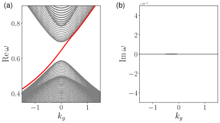
Figure 2: The spectrum of operator $\mathcal{H}$. The real and imaginary parts of the spectrum are shown in (a) and (b), respectively. The spectral flow, i.e., the TASW, is depicted in red, the bulk modes are depicted in gray. In (b), the imaginary parts of all modes are smaller than $10^{-8}$.

To verify the existence of TASW, we study the full spectrum of $\mathcal{H}$ numerically. In a 1D domain $[0,L]$, let $v_{\mathrm{A}}(x)=v_{\mathrm{A2}}+0.5(v_{\mathrm{A1}}-v_{\mathrm{A2}})[1+\tanh(\frac{L/2-x}{l})]$, where $v_{\mathrm{A1}},v_{\mathrm{A2}}$ are the Alfvén velocities in the two bulk regions, $L$ is the system size, $l$ controls the width of the interface, and $v_{\mathrm{s}}$ is determined from Eq. (25). The ratio between two velocities $\zeta(x)$ plays the role of a system parameter, similar to the parameter $m(x)$ in Fig. 1. As an example, we choose $v_{\mathrm{A1}}=1,v_{\mathrm{A2}}=0.85,v_{\mathrm{s1}}=0.4,v_{\mathrm{s2}}=0.625,L=100,l=2,d_{\mathrm{i}}=1,$ and $k_{z}=1.25$. The Weyl point locates at $\zeta=0.55$. Because in the two bulk regions $\zeta_{1}=0.4$, $\zeta_{2}=0.73$, we shall expect a degeneracy point somewhere in the interface region. The numerical scheme to calculate the spectrum of operator $\mathcal{H}$ is similar to that in Ref. [22]. The real part of the spectrum displayed in Fig. 2(a) clearly shows a spectral flow, i.e., the TASW, and Fig. 2(b) confirms that the spectrum is real ($|\mathrm{Im}\,\omega|<10^{-8}$). These numerical results agree with our theoretical prediction developed above. The TASW can also be faithfully modeled by a titled Dirac cone [23](see Appendix C).

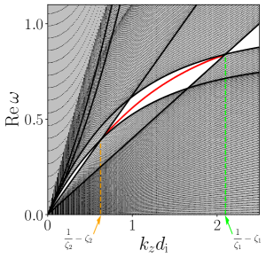
Figure 3: The numerically calculated spectrum of operator $\mathcal{H}$ as a function of $k_{z}$ at $k_{y}=0$. The bulk modes are depicted in black dots, the topological edge mode, i.e., the TASEW, by depicted in red dots. For clarity, the bulk region are filled in gray; while the frequency gap of bulk waves are filled in white. The black lines represent the dispersion relations in two bulk regions calculated from Eq. (26) at $k_{\perp}=0$. The locations of two degeneracy points are labeled in orange and green dashed lines. The red spectral flow curve resembles the Fermi arc in topological electronic crystals.

For a given equilibrium profile with fixed $\zeta_{1}=v_{\mathrm{s1}}/v_{\mathrm{A1}}$ and $\zeta_{2}=v_{\mathrm{s2}}/v_{\mathrm{A2}}$, Eq. (27) can be solved to find the following range of $k_{z}$ where the TASW exists,

$$\dfrac{1}{\zeta_{2}}-\zeta_{2}<k_{z}d_{\mathrm{i}}<\dfrac{1}{\zeta_{1}}-\zeta_{1}.$$ (28)

In Fig. 3, this condition is numerically verified by the numerically calculated spectrum of $\mathcal{H}$ at different $k_{z}$ with $k_{y}=0$. A frequency gap exists at all $k_{z}$ except for the Weyl points. However, the spectral flow, which is depicted in red, only shows up in the region where condition (28) is satisfied. It resembles the Fermi arc in topological electronic crystals. These numerical results verify that in the Hall MHD model, the dispersion relation of the asymptotic symbol $H_{0}$ can accurately predict the topological edge modes admitted by a PT-symmetric non-Hermitian operator $\mathcal{H}$.

Conclusions and discussion

In conclusion, we studied topological edge modes and spectral flows in non-Hermitian inhomogeneous continuous media that are PT-symmetric and asymptotically Hermitian. For these media, if the asymptotic symbol $H_{0}$ supports a Weyl point of two-fold degeneracy, then the non-Hermitian operator $\mathcal{H}$ of system admits topological edge modes with real frequency, as characterized by a spectral flow near the Weyl point. The spectral-flow index of the modes is determined by $H_{0}.$ As an application of the general theory developed, we identified a topological edge mode called topological Alfvén-sound wave in the non-Hermitian Hall MHD model. The analysis reported in this paper could be applied to search for topological modes in a wide range of non-Hermitian PT-symmetric inhomogeneous continuous media in fluids and plasmas.

Appendix A Spectra of the two-band model with anti-Hermitian parts

In this appendix, we calculate the spectra and the eigenmodes of the following class of Hamiltonian operators,

$$\mathcal{H}[\lambda;x,\partial_{x}] =\begin{pmatrix}f(x)/\kappa&\lambda-\partial_{x}\\ \lambda+\partial_{x}&-\kappa f(x)\end{pmatrix}+\mathrm{i}g(x)\sigma^{\alpha}$$ (29)

$$\doteq\mathcal{H}_{\mathrm{H}}+\mathrm{i}\mathcal{H}_{\mathrm{A}}.$$ (30)

Here, $f(x)$ and $g(x)$ are real functions of $x$, and $\lambda$ is a constant control parameter. The parameter $\kappa$ measures the tilting of the Dirac operator [23], indicating that $f(x)$ is associated to both $\sigma^{z}$ and $\sigma^{0}$. Equation (2) corresponds to the case where $\kappa=1$ and $g(x)=\epsilon f^{\prime}(x)$. We first give the analytical solutions for several special cases, and then provide numerically solved examples for general $f$ and $g$.

A.1 Analytical solution without anti-Hermitian part

When $f(x)=x$ and $g=0$, the operator only has a Hermitian part,

$$\mathcal{H}_{\mathrm{H}}=\begin{pmatrix}x/\kappa&\lambda-\partial_{x}\\ \lambda+\partial_{x}&-\kappa x\end{pmatrix},$$ (31)

which can be analytically solved using the techniques given in Refs. [26, 23, 27]. Let $R=\mathrm{diag}(\kappa,1)$, we have

$$\mathcal{H}_{\mathrm{H}}^{\prime}=R^{-1}\mathcal{H}_{\mathrm{H}}R=\begin{pmatrix}{x}/\kappa&(\lambda-\partial_{x})/\kappa\,\\ \kappa(\lambda+\partial_{x})&-\kappa{x}\end{pmatrix}$$ (32)

Define the following variables for convenience,

$$\mu_{1}\doteq\dfrac{1}{2}\left(\kappa+\dfrac{1}{\kappa}\right),\quad\mu_{2}\doteq\dfrac{1}{2}\left(\kappa-\dfrac{1}{\kappa}\right).$$ (33)

In terms of Pauli matrices,

$$\mathcal{H}_{\mathrm{H}}^{\prime}=-\mu_{2}x\sigma^{0}+(\mu_{2}\partial_{x}+\mu_{1}\lambda)\sigma^{x}-\mathrm{i}(\mu_{1}\partial_{x}+\mu_{2}\lambda)\sigma^{y}+\mu_{1}x\sigma^{z}.$$ (34)

Making a cyclic rotation of Pauli matrices $(\sigma^{0},\sigma^{x},\sigma^{y},\sigma^{z})\to(\sigma^{0},\sigma^{z},\sigma^{x},\sigma^{y})$ through a similarity transformation, $\mathcal{H}_{\mathrm{H}}^{\prime}$ is transformed to

$$\mathcal{H}_{\mathrm{H}}^{\prime} =-\mu_{2}x\sigma^{0}+(\mu_{2}\partial_{x}+\mu_{1}\lambda)\sigma^{z}-\mathrm{i}(\mu_{1}\partial_{x}+\mu_{2}\lambda)\sigma^{x}+\mu_{1}x\sigma^{y}.$$ (35)

$$=\begin{pmatrix}\mu_{1}\lambda-\sqrt{2}\mu_{2}\hat{a}^{\dagger}&\mathrm{i}(-\mu_{2}\lambda-\sqrt{2}\mu_{1}\hat{a})\\ \mathrm{i}(-\mu_{2}\lambda+\sqrt{2}\mu_{1}\hat{a}^{\dagger})&-\mu_{1}\lambda-\sqrt{2}\mu_{2}\hat{a}\end{pmatrix}.$$ (36)

Here,

$$\hat{a}\doteq\frac{1}{\sqrt{2}}\left(x+\partial_{x}\right),\quad\hat{a}^{\dagger}\doteq\frac{1}{\sqrt{2}}\left(x-\partial_{x}\right)$$ (37)

are the ladder operators.

Define functions $|n;\delta\rangle$ as

$$\langle x|n;\delta\rangle\doteq\varphi_{n}(x+\sqrt{2}\delta),\quad\varphi_{n}(x)\doteq\frac{1}{\left(2^{n}n!\sqrt{\pi}\right)^{1/2}}\mathrm{e}^{-{x^{2}}/{2}}H_{n}(x),$$ (38)

where $H_{n}(x)$ is the $n$-th Hermite polynomial. The eigenvectors of the bulk modes of $\mathcal{H}"_{\mathrm{H}}$ are

$$\Psi_{n}^{\pm}=\begin{pmatrix}|n;\delta_{n}^{\pm}\rangle\\ \mathrm{i}\gamma_{n}^{\pm}|n+1;\delta_{n}^{\pm}\rangle\end{pmatrix},\quad n=0,1,2,\ldots,$$ (39)

where

$$\gamma_{n}^{\pm}=\dfrac{-\lambda\pm\sqrt{\lambda^{2}+n+1}}{\sqrt{n+1}},\quad\delta_{n}^{\pm}=\mp\dfrac{\mu_{2}}{\mu_{1}}\sqrt{\lambda^{2}+n+1}.$$ (40)

The corresponding eigenvalues are

$$\omega_{n}^{\pm}=\pm\dfrac{2\sqrt{2}\kappa}{1+\kappa^{2}}\sqrt{\lambda^{2}+n+1}.$$ (41)

We also find the eigenvector and eigenvalue of the spectral flow of $\mathcal{H}"_{\mathrm{H}}$, labeled by $n=-1$, to be

$$\Psi_{-1}=\begin{pmatrix}0\\ |0,\delta_{-1}\rangle\end{pmatrix},\quad\delta_{-1}=\dfrac{\mu_{2}}{\mu_{1}}\lambda,\quad\omega_{-1}=-\dfrac{2\sqrt{2}\kappa}{1+\kappa^{2}}\lambda.$$ (42)

A.2 Analytical solutions with anti-Hermitian parts

Here, we assume $f(x)=x,\,g(x)=f^{\prime}(x)=1$ and study the eigenvalues and eigenvectors of the Hamiltonian operator $\mathcal{H}$ in Eq. (29) with different $\mathrm{i}\sigma^{\alpha}$. We will see that when $\kappa\neq 1$, only the $\mathcal{H}$ with $\mathrm{i}\sigma^{y}$ renders the system PT-symmetric.

1. $\mathcal{H}$ with $\mathrm{i}\sigma^{0}$. Since $\mathrm{i}\sigma^{0}$ does not depend on $x$, the addition of $\mathrm{i}\sigma^{0}$ only shifts the eigenvalue by $\mathrm{i}$,

$$\begin{cases}\omega_{n}^{\pm}=\pm\dfrac{2\sqrt{2}\kappa}{1+\kappa^{2}}\sqrt{\lambda^{2}+n+1}+\mathrm{i},\qquad n=0,1,2,\cdots,\\[10.0pt] \omega_{-1}=-\dfrac{2\sqrt{2}\kappa}{1+\kappa^{2}}\lambda+\mathrm{i}.\end{cases}$$ (43)

2. $\mathcal{H}$ with $\mathrm{i}\sigma^{x}$. In terms of slightly modified control parameter $\tilde{\lambda}\doteq\lambda+\mathrm{i}$,

$$\mathcal{H}=\begin{pmatrix}x/\kappa&\tilde{\lambda}-\partial_{x}\\ \tilde{\lambda}+\partial_{x}&-\kappa x\end{pmatrix}.$$ (44)

Therefore, the eigenvalues are

$$\begin{cases}\omega_{n}^{\pm}=\pm\dfrac{2\sqrt{2}\kappa}{1+\kappa^{2}}\sqrt{(\lambda+\mathrm{i})^{2}+n+1},\qquad n=0,1,2,\cdots,\\[10.0pt] \omega_{-1}=-\dfrac{2\sqrt{2}\kappa}{1+\kappa^{2}}(\lambda+\mathrm{i}).\end{cases}$$ (45)

3. $\mathcal{H}$ with $\mathrm{i}\sigma^{y}$. By applying the technique described in the main text, the anti-Hermitian part $\mathrm{i}\sigma^{y}$ in operator $\mathcal{H}$ can be removed by a similarity transformation $\mathcal{H\rightarrow}e^{-x}\mathcal{H}e^{x}$. The eigenvalues thus do not change after adding $\mathrm{i}\sigma^{y}$. Noticeably, the factor $e^{-x}$ in the eigenvectors resembles the “non-Hermitian skin effect” [36, 37] found in general non-Hermitian systems. However, in the given example, eigenvectors are already localized at the interface due to the factor $e^{-x^{2}/2}$ in Eq. (38), even in the Hermitian case.

4. $\mathcal{H}$ with $\mathrm{i}\sigma^{z}$. In terms of modified variable $\tilde{x}\doteq x+\mathrm{i}/\mu_{1}$, the operator is

$$\mathcal{H}=\begin{pmatrix}\tilde{x}/\kappa&\lambda-\partial_{\tilde{x}}\\ \lambda+\partial_{\tilde{x}}&-\kappa\tilde{x}\end{pmatrix}+\dfrac{\mu_{2}}{\mu_{1}}\mathrm{i}\sigma^{0}.$$ (46)

The eigenvalues are shifted by $\mathrm{i}\mu_{2}/\mu_{1}$, similar to the case of $\mathcal{H}$ with $\mathrm{i}\sigma^{0}$. When $\kappa=1$, the operator is not tilted, and the addition of $\mathrm{i}\sigma^{z}$ does not introduce an imaginary part.

A.3 Numerical solutions with anti-Hermitian parts

Here we present several numerical results on the spectra of $\mathcal{H}$ in Eq. (29) for the case of $f(x)=m(x)$, $g(x)=\epsilon m^{\prime}(x)$, and

$$m(x)\doteq\tanh\left(\dfrac{x-L/4}{l}\right)-\tanh\left(\dfrac{x-3L/4}{l}\right)-1.$$ (47)

Here, $L$ is the system length, $l$ is the scale length of the interface region. $m(x)$ and $m^{\prime}(x)$ are plotted in Fig. 4. The $x$-direction is chosen to be periodic with periodicity $L$. In the bulk region around $x=L/2$ and $x=0$, $m^{\prime}=0$ and the system is homogeneous. In the interface region at $x=L/4$ and $x=3L/4$, $m^{\prime}(x)\neq 0$ and system is non-Hermitian.

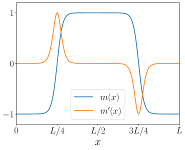
Figure 4: $m(x)$ and $m^{\prime}(x)$.

In the numerical example, we choose $L=30,l=1,$ and $\kappa=2$. The spectrum of the Hermitian operator at $\epsilon=0$ is shown in Fig. 5. Since there are two interface regions at $x=L/4$ and $x=3L/4$, there are two spectral flows indicated by the blue and red dots.

Figure 5: The spectrum of Hermitian operators. Grey dots indicate bulk mods, red/blue dots indicate topological edge modes (spectral flow) localized at the left/right interface.

For the non-Hermitian case, we choose $\epsilon=0.1$, so that the real part of the spectrum of $\mathcal{H}$ does not deviate significantly from its Hermitian counterpart. With different anti-Hermitian parts $\mathrm{i}\sigma^{\alpha}$, the real parts of the spectrum are qualitatively similar to Fig. 5. The imaginary parts are shown in Fig. 6.

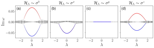
Figure 6: The imaginary part of operator $\mathcal{H}$ in Eq. (29), whose anti-Hermitian part $\mathcal{H}_{\mathrm{A}}$ is proportional to (a) $\sigma^{0}$, (b) $\sigma^{x}$, (c) $\sigma^{y}$, and (d) $\sigma^{z}$. The gray points indicate bulk modes, the blue/red points indicate edge modes localized at left/right edge. In (b) and (c), the blue and red points coincide.

We observe that with anti-Hermitian terms proportional to $\mathrm{i}\sigma^{0},\,\mathrm{i}\sigma^{x}$ or $\mathrm{i}\sigma^{z}$, the spectrum of $\mathcal{H}$, including its spectral flow, are complex. The effect of $\mathrm{i}\sigma^{0}$ and $\mathrm{i}\sigma^{z}$ are similar, akin to the analytical solutions given above. However, with an anti-Hermitian term proportional to $\mathrm{i}\sigma^{y}$, $\mathcal{H}$ is PT-symmetric, and its spectrum is still real.

Appendix B The Hall MHD model

Within the MHD model, which focuses on low frequency and long-wavelength phenomena, the displacement current $\partial_{t}\mathbf{E}$ in Maxwell’s equations is ignored. When studying plasma waves, the dynamics of plasma is usually assumed to be adiabatic with the equation of state $p/\rho^{\gamma}=\mathrm{Const.}$, where $p$ is plasma pressure, $\rho$ is plasma mass density, and $\gamma$ is ratio of specific heats. With this assumption, the equations of motions for $\rho,$ $\mathbf{v}$, $\mathbf{B}$, and $p$ are

$$\partial_{t}\rho+\nabla\cdot(\rho\mathbf{v})=0,$$ (48)

$$\rho\dfrac{\mathrm{d}\mathbf{v}}{\mathrm{d}t}=\mathbf{j}\times\mathbf{B}-\nabla p,$$ (49)

$$\partial_{t}\mathbf{B}=-\nabla\times\mathbf{E},$$ (50)

$$\dfrac{\mathrm{d}p}{\mathrm{d}t}=-\gamma p\nabla\cdot\mathbf{v},$$ (51)

where $\mathbf{v}$ is the plasma macroscopic velocity, and $\mathrm{d}/\mathrm{d}t\doteq\partial_{t}+\mathbf{v}\cdot\nabla$. The plasma current $\mathbf{j}$ is related to the magnetic field $\mathbf{B}$ by the Ampere’s law

$$\quad\mu_{0}\mathbf{j}=\nabla\times\mathbf{B},$$ (52)

where $\mu_{0}$ is the vacuum permeability. Since the displacement current is ignored, $\mathbf{E}$ is obtained from the generalized Ohm’s law. Different forms of Ohm’s laws lead to different MHD models. In the Hall MHD approximation, the electron inertia is ignored ($m_{\mathrm{e}}\to 0$) and the plasma is assumed to be infinitely conductive. The Ohm’s law could be written as [47]

$$\mathbf{E}+\mathbf{v}\times\mathbf{B}=\dfrac{\mathbf{j}\times\mathbf{B}-\nabla p_{\mathrm{e}}}{n_{\mathrm{e}}e},$$ (53)

where $e>0$ is the elementary charge, $n_{\mathrm{e}}$ is the electron number density, $p_{\mathrm{e}}$ is the electron pressure.

Combining Faraday’s law and Ohm’s law, we can eliminate electric field $\mathbf{E}$

$$\partial_{t}\mathbf{B}=\nabla\times(\mathbf{v}\times\mathbf{B})-\nabla\times\left(\dfrac{\mathbf{j}\times\mathbf{B}}{n_{\mathrm{e}}e}\right)+\nabla\times\left(\dfrac{\nabla p_{\mathrm{e}}}{n_{\mathrm{e}}e}\right).$$ (54)

If the electrons are assumed to be barotropic [47], i.e., the electron pressure is a function of electron number density, $p_{\mathrm{e}}=p_{\mathrm{e}}(n_{\mathrm{e}})$, the last term in Eq. (54) vanishes.

Consider an equilibrium without flow and with homogeneous densities $\rho$ and $n_{\mathrm{e}}$. Hereafter, we use symbols without subscripts such $\mathbf{B}$, $p$, and $\mathbf{j}$ to indicate equilibrium, time-independent fields. From Eq. (49), the equilibrium fields $\mathbf{B}$ and $p$ satisfy the pressure balance,

$$\nabla p=\mathbf{j}\times\mathbf{B}=\dfrac{1}{\mu_{0}}(\nabla\times\mathbf{B})\times\mathbf{B}.$$ (55)

For a given equilibrium, the perturbed field $\left(\rho_{1},\mathbf{v}_{1},\mathbf{B}_{1},\mathbf{p}_{1}\right)$ are governed by the linearized system,

$$\partial_{t}\rho_{1} =-\rho\nabla\cdot\mathbf{v}_{1},$$ (56)

$$\rho\partial_{t}\mathbf{v}_{1} =\mathbf{j}_{1}\times\mathbf{B}+\mathbf{j}\times\mathbf{B}_{1}-\nabla p_{1},$$ (57)

$$\partial_{t}\mathbf{B}_{1} =\nabla\times(\mathbf{v}_{1}\times\mathbf{B})-\dfrac{1}{en_{e}}\nabla\times(\,\mathbf{j}_{1}\times\mathbf{B}+\mathbf{j}\times\mathbf{B}_{1}),$$ (58)

$$\partial_{t}p_{1} =-\mathbf{v}_{1}\cdot\nabla p-\gamma p\nabla\cdot\mathbf{v}_{1}.$$ (59)

Equation (56) is decoupled from the others. In terms of the following normalized variables

$$\tilde{\mathbf{v}}\doteq\sqrt{\rho}\mathbf{v}_{1},\quad\tilde{\mathbf{B}}\doteq\dfrac{\mathbf{B}_{1}}{\sqrt{\mu_{0}}},\quad\tilde{p}\doteq\dfrac{p_{1}}{\sqrt{\gamma p}},$$ (60)

the linearized equations become are

$$\partial_{t}\tilde{\mathbf{v}} =(\nabla\times\tilde{\mathbf{B}})\times\mathbf{v}_{\mathrm{A}}+(\nabla\times\mathbf{v}_{\mathrm{A}})\times\tilde{\mathbf{B}}-\nabla(v_{\mathrm{s}}\tilde{p}),$$ (61)

$$\partial_{t}\tilde{\mathbf{B}} =\nabla\times(\tilde{\mathbf{v}}\times\mathbf{v}_{\mathrm{A}})-\sqrt{\dfrac{\rho}{\mu_{0}}}\dfrac{1}{n_{\mathrm{e}}e}\nabla\times\left[(\nabla\times\tilde{\mathbf{B}})\times\mathbf{v}_{\mathrm{A}}+(\nabla\times\mathbf{v}_{\mathrm{A}})\times\tilde{\mathbf{B}}\right],$$ (62)

$$\partial_{t}\tilde{p} =-v_{\mathrm{s}}\nabla\cdot\tilde{\mathbf{v}}-(2/\gamma)\tilde{\mathbf{v}}\cdot\nabla v_{\mathrm{s}},$$ (63)

where

$$\mathbf{v}_{\mathrm{A}}\doteq\dfrac{\mathbf{B}}{\sqrt{\mu_{0}\rho}},\quad v_{\mathrm{s}}\doteq\sqrt{\dfrac{\gamma p}{\rho}}$$ (64)

are Alfvén velocity and sound velocity. Let $n_{\mathrm{i}},m_{\mathrm{i}},q_{\mathrm{i}}$ denote the number density, mass, and charge of ions. Using the quasi-neutrality condition $n_{\mathrm{e}}e=n_{\mathrm{i}}q_{\mathrm{i}}$, the coefficient $\sqrt{\rho\mu_{0}/n_{\mathrm{e}}e}$ in Eq. (62) can be simplified as

$$\sqrt{\dfrac{\rho}{\mu_{0}}}\dfrac{1}{n_{\mathrm{e}}e}=\sqrt{\dfrac{n_{\mathrm{i}}m_{\mathrm{i}}}{1/(\varepsilon_{0}c^{2})}}\dfrac{1}{n_{\mathrm{i}}q_{\mathrm{i}}}=c\left/\sqrt{\dfrac{n_{\mathrm{i}}q_{\mathrm{i}}^{2}}{\varepsilon_{0}m_{\mathrm{i}}}}\right.=\dfrac{c}{\omega_{\mathrm{pi}}}=d_{\mathrm{i}},$$ (65)

where $\epsilon_{0}$ is the vacuum permittivity, $c$ is the light speed, $\omega_{\mathrm{pi}}$ is the ion plasma frequency, and $d_{\mathrm{i}}$ is known as the ion skin depth. The final linearized equations for Hall MHD become Eqs. (20)-(22) in the main text. In the limit of $d_{\mathrm{i}}\to 0$, the system reduces to the ideal MHD model where the right-hand of Eq. (53) vanishes.

To study the dispersion relation and wave topology in the bulk region, we assume the equilibrium magnetic field $\mathbf{B}$ and pressure $p$ are constants. In this case, the wave fields $\Psi=(\tilde{\mathbf{v}},\tilde{\mathbf{B}},\tilde{p})^{\intercal}$ are governed by $\mathrm{i}\partial_{t}\Psi=\mathcal{H}_{0}\Psi$, where $\mathcal{H}_{0}$ is the asymptotic Hamiltonian shown in Eq. (24). The corresponding symbol is

$${H}_{0}=\begin{pmatrix}0&(\mathbf{v}_{\mathrm{A}}\mathbf{k})^{\intercal}-\mathbf{v}_{\mathrm{A}}{\cdot}\mathbf{k}\,\,&v_{\mathrm{s}}\mathbf{k}\\[3.0pt] (\mathbf{v}_{\mathrm{A}}\mathbf{k})-\mathbf{v}_{\mathrm{A}}{\cdot}\mathbf{k}\,\,&\mathrm{i}d_{\mathrm{i}}(\mathbf{v}_{\mathrm{A}}{\cdot}\mathbf{k})\mathbf{k}\times&0\\[3.0pt] v_{\mathrm{s}}\mathbf{k}^{\intercal}&0&0\end{pmatrix}.$$ (66)

It is clear that $H_{0}$ and $\mathcal{H}_{0}$ are Hermitian.

Let magnetic field is in the $z$-direction and $\mathbf{v}_{\mathrm{A}}=v_{\mathrm{A}}\mathbf{e}_{z}$. $H_{0}$ has one zero eigenvalue $\omega_{0}=0$, whose eigenvector is $\Psi=(0,0,0,0,0,1,0)^{\intercal}$. The rest 6 eigenvalues are given by Eq. (26). Because $\omega$ only appears in terms of $\omega^{2}$ in Eq. (26), the eigenvalues are symmetric with respect to zero. We can thus only study the three positive frequency branches. They are called fast wave, Alfvén wave, and slow wave according to their phase velocities, which satisfies the following order,

$$v_{\mathrm{p,slow}}\leq v_{\mathrm{p,Alfven}}\leq v_{\mathrm{p,fast}}.$$ (67)

The dispersion relation is plotted in Figs. 7 and 8. Since $k_{x}$ and $k_{y}$ contribute symmetrically through $k_{\perp}^{2}\doteq k_{x}^{2}+k_{y}^{2}$, the eigenvalues $\omega_{n}$ are plotted as functions of $(k_{\perp},k_{z})$.

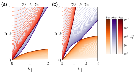
Figure 7: Dispersion relations of three positive frequency branches. The red, purple and orange lines represent the fast, Alfvén, and slow waves, respectively. The saturation level of each color represents the value of $k_{\perp}$. There are two types of Weyl points depending on the ratio between $v_{\mathrm{s}}$ and $v_{\mathrm{A}}$.

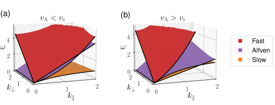
Figure 8: The 3D rendition of the dispersion relations in Fig. 7.

From the dispersion relations, we observe that a Weyl point can be formed by the crossing between the fast and Alfvén waves or between the slow and Alfvén waves. The Weyl point can be analytically solved for from Eq. (26). When $k_{\perp}=0$, Eq. (26) has three positive solutions,

$$\omega_{1}=v_{s}k_{z},\qquad\omega_{2,3}=v_{\mathrm{A}}k_{z}\left(\sqrt{1+\dfrac{1}{4}k_{z}^{2}d_{\mathrm{i}}^{2}}\pm\dfrac{1}{2}k_{z}d_{\mathrm{i}}\right).$$ (68)

The value of $k_{z}$ at the Weyl points can be expressed in terms of $\zeta=v_{\mathrm{s}}/v_{\mathrm{A}}$,

$$k_{z}d_{\mathrm{i}}=\left|\dfrac{1}{\zeta}-\zeta\right|=\begin{cases}{1}/{\zeta}-\zeta,\quad\text{when: }\zeta<1,\\[3.0pt] \zeta-{1}/{\zeta},\quad\text{when: }\zeta>1.\end{cases}$$ (69)

If $k_{z}$ is fixed, the value of $\xi$ at the Weyl points is

$$\zeta=\sqrt{1+\dfrac{1}{4}k_{z}^{2}d_{\mathrm{i}}^{2}}\pm\dfrac{1}{2}k_{z}d_{\mathrm{i}}.$$ (70)

For a fixed $k_{z}$, the topological charge of each Weyl point can be calculated in the parameter space $(x,k_{x},k_{y})$, which is given explicitly using a two-band approximation in Appendix C.

Appendix C The topological Alfvén-sound wave in Hall MHD

In this appendix, we provide detailed derivations of the topological Alfvén-sound wave in Hall MHD.

In an inhomogeneous equilibrium, the operator $\mathcal{H}$ is relatively complicated. From Eqs. (20)-(22), the operator $\mathcal{H}$ can be written in a $7\times 7$ matrix,

$$\mathcal{H} =\mathcal{H}_{0}+{\color[rgb]{0,0,1}\mathcal{H}_{1}}+{\color[rgb]{1,0,0}\mathcal{H}_{2}}$$ (71)

$$= \left(\begin{array}[]{ccc}0&h_{12}&h_{13}\\ h_{21}&h_{22}&0\\ h_{31}&0&0\end{array}\right),$$ (75)

where

$$h_{12} =\left(\begin{array}[]{ccc}-v_{\mathrm{A}}k_{z}&0&-\mathrm{i}v_{\mathrm{A}}\partial_{x}{\color[rgb]{0,0,1}-\mathrm{i}v_{\mathrm{A}}^{\prime}}\\ 0&-v_{\mathrm{A}}k_{z}&v_{\mathrm{A}}k_{y}\\ {\color[rgb]{0,0,1}\mathrm{i}v_{\mathrm{A}}^{\prime}}&0&0\end{array}\right),$$ (79)

$$h_{13} =\left(\begin{array}[]{c}-\mathrm{i}v_{\mathrm{s}}\partial_{x}{\color[rgb]{0,0,1}-\mathrm{i}v_{\mathrm{s}}^{\prime}}\\ v_{\mathrm{s}}k_{y}\\ v_{\mathrm{s}}k_{z}\end{array}\right),$$ (83)

$$h_{21} =\left(\begin{array}[]{ccc}-v_{\mathrm{A}}k_{z}&0&0\\ 0&-v_{\mathrm{A}}k_{z}&0\\ -\mathrm{i}v_{\mathrm{A}}\partial_{x}{\color[rgb]{0,0,1}-\mathrm{i}v_{\mathrm{A}}^{\prime}}&v_{\mathrm{A}}k_{y}&0\end{array}\right),$$ (87)

$$h_{22} =\left(\begin{array}[]{ccc}{\color[rgb]{0,0,1}d_{\mathrm{i}}v_{\mathrm{A}}^{\prime}k_{y}}&-\mathrm{i}d_{\mathrm{i}}v_{\mathrm{A}}k_{z}^{2}&\mathrm{i}d_{\mathrm{i}}v_{\mathrm{A}}k_{y}k_{z}\\ \mathrm{i}d_{\mathrm{i}}v_{\mathrm{A}}k_{z}^{2}{\color[rgb]{1,0,0}+\mathrm{i}d_{\mathrm{i}}v_{\mathrm{A}}^{\prime\prime}}&{\color[rgb]{0,0,1}d_{\mathrm{i}}v_{\mathrm{A}}^{\prime}k_{y}}&-k_{z}d_{\mathrm{i}}v_{\mathrm{A}}\partial_{x}\\ -\mathrm{i}d_{\mathrm{i}}v_{\mathrm{A}}k_{y}k_{z}&d_{\mathrm{i}}k_{z}v_{\mathrm{A}}\partial_{x}{\color[rgb]{0,0,1}+d_{\mathrm{i}}k_{z}v_{\mathrm{A}}^{\prime}}&0\end{array}\right),$$ (91)

$$h_{31} =\left(\begin{array}[]{ccc}-\mathrm{i}v_{\mathrm{s}}\partial_{x}{\color[rgb]{0,0,1}-\mathrm{i}(2/\gamma)v_{\mathrm{s}}^{\prime}}&v_{\mathrm{s}}k_{y}&v_{\mathrm{s}}k_{z}\end{array}\right).$$ (93)

Here, $\mathcal{H}_{0}$ is the asymptotic Hamiltonian that depends on $v_{\mathrm{A}}$ and $v_{\mathrm{s}}$, but not their derivatives. It is the same as Eq. (24) in the main text. The terms that show up in $\mathcal{H}_{0}$ are written in black. We can see that $\mathcal{H}$ is significantly different from $\mathcal{H}_{0}$ in the inhomogeneous region. $\mathcal{H}_{1}$, which are highlighted in blue, depends on the first order derivatives. Similarly, $\mathcal{H}_{2}$, highlighted in red, depends on the second order derivatives. It is clear that $\mathcal{H}$ is not Hermitian due to the background inhomogeneity. The anti-Hermitian part of $\mathcal{H}$ is

$$\mathcal{H}_{\mathrm{A}}\doteq\dfrac{1}{2\mathrm{i}}(\mathcal{H}-\mathcal{H}^{\dagger})=\left(\begin{array}[]{ccc|ccc|c}0&0&0&0&0&-v_{\mathrm{A}}^{\prime}/2&-v_{\mathrm{s}}^{\prime}/\gamma\\ 0&0&0&0&0&0&0\\ 0&0&0&v_{\mathrm{A}}^{\prime}/2&0&0&0\\ \hline\cr 0&0&v_{\mathrm{A}}^{\prime}/2&0&{d}_{\mathrm{i}}v_{\mathrm{A}}^{\prime\prime}/2&0&0\\ 0&0&0&{d}_{\mathrm{i}}v_{\mathrm{A}}^{\prime\prime}/2&0&0&0\\ -v_{\mathrm{A}}^{\prime}/2&0&0&0&0&0&0\\ \hline\cr-v_{\mathrm{s}}^{\prime}/\gamma&0&0&0&0&0&0\end{array}\right)$$ (101)

Notice that for a real function $f(x)$,

$$\left[\mathrm{i}f(x)\dfrac{\mathrm{d}}{\mathrm{d}x}\right]^{\dagger}=\mathrm{i}f^{\prime}(x)+\mathrm{i}f(x)\dfrac{\mathrm{d}}{\mathrm{d}x}.$$ (102)

Although $\mathcal{H}$ is not Hermitian, it is PT-symmetric for $\mathcal{P}=\mathrm{diag}(-1,1,1,-1,1,1,1)$ and $\mathcal{T}$ being complex conjugation, i.e., $\mathcal{PT}\mathcal{H}\mathcal{TP}=\mathcal{P}\mathcal{H}^{*}\mathcal{P}=\mathcal{H}$. To prove this property, the effect of $\mathcal{P}$ and $\mathcal{T}$ operators on $\mathcal{H}$ are graphically shown in Fig. 9. Each element in Eq. (71) is either real or imaginary. Under time reversal or parity transform, the sign of each element is either unchanged or flipped. Observe that $\mathcal{P}$ and $\mathcal{T}$ have the same effect on $\mathcal{H}$. Thus, their combination keeps $\mathcal{H}$ unchanged.

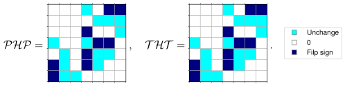
Figure 9: The effects of $\mathcal{P}$ and $\mathcal{T}$ operators on $\mathcal{H}$. The elements of $\mathcal{H}$ are represented by a $7\times 7$ grids. Vanishing elements are shown in white. Elements that are unchanged under an operator are shown in light blue. Elements that have their sign flipped under an operator are shown in dark blue.

For a function $f(x)$ and operator $\hat{k}=-\mathrm{i}\partial_{x}$, their Wigner-Weyl transforms are

$$\mathscr{W}[f(x)]=f(x),\quad\mathscr{W}[\hat{k}]=k,\quad\mathscr{W}[f(x)\hat{k}]=f(x)k+\mathrm{i}f^{\prime}(x)/2.$$ (103)

From these relations, the symbol of $\mathcal{H}$ in Eq. (71) is

$$H =\mathscr{W}[\mathcal{H}]=H_{0}+{\color[rgb]{0,0,1}H_{1}}+{\color[rgb]{1,0,0}H_{2}}$$ (104)

$$=\left(\begin{array}[]{ccc}0&s_{12}&s_{13}\\ s_{21}&s_{22}&0\\ s_{31}&0&0\end{array}\right),$$ (108)

where

$$s_{12} =\left(\begin{array}[]{ccc}-v_{\mathrm{A}}k_{z}&0&v_{\mathrm{A}}k_{x}{\color[rgb]{0,0,1}-\frac{\mathrm{i}}{2}v_{\mathrm{A}}^{\prime}}\\ 0&-v_{\mathrm{A}}k_{z}&v_{\mathrm{A}}k_{y}\\ {\color[rgb]{0,0,1}\mathrm{i}v_{\mathrm{A}}^{\prime}}&0&0\end{array}\right),$$ (112)

$$s_{13} =\left(\begin{array}[]{c}v_{\mathrm{s}}k_{x}{\color[rgb]{0,0,1}-\frac{\mathrm{i}}{2}v_{\mathrm{s}}^{\prime}}\\ v_{\mathrm{s}}k_{y}\\ v_{\mathrm{s}}k_{z}\end{array}\right),$$ (116)

$$s_{21} =\left(\begin{array}[]{ccc}-v_{\mathrm{A}}k_{z}&0&0\\ 0&-v_{\mathrm{A}}k_{z}&0\\ v_{\mathrm{A}}k_{x}{\color[rgb]{0,0,1}-\frac{\mathrm{i}}{2}v_{\mathrm{A}}^{\prime}}&v_{\mathrm{A}}k_{y}&0\end{array}\right),$$ (120)

$$s_{22} =\left(\begin{array}[]{ccc}{\color[rgb]{0,0,1}d_{\mathrm{i}}v_{\mathrm{A}}^{\prime}k_{y}}&-\mathrm{i}d_{\mathrm{i}}v_{\mathrm{A}}k_{z}^{2}&\mathrm{i}d_{\mathrm{i}}v_{\mathrm{A}}k_{y}k_{z}\\ \mathrm{i}d_{\mathrm{i}}v_{\mathrm{A}}k_{z}^{2}{\color[rgb]{1,0,0}+\mathrm{i}d_{\mathrm{i}}v_{\mathrm{A}}^{\prime\prime}}&{\color[rgb]{0,0,1}d_{\mathrm{i}}v_{\mathrm{A}}^{\prime}k_{y}}&-k_{z}d_{\mathrm{i}}v_{\mathrm{A}}\partial_{x}\\ -\mathrm{i}d_{\mathrm{i}}v_{\mathrm{A}}k_{y}k_{z}&\mathrm{i}d_{\mathrm{i}}v_{\mathrm{A}}k_{x}k_{z}{\color[rgb]{0,0,1}+\frac{d_{\mathrm{i}}}{2}v_{\mathrm{A}}^{\prime}k_{z}}&0\end{array}\right),$$ (124)

$$s_{31} =\left(\begin{array}[]{ccc}v_{\mathrm{s}}k_{x}{\color[rgb]{0,0,1}+\mathrm{i}(\frac{1}{2}-\frac{2}{\gamma})v_{\mathrm{s}}^{\prime}}&v_{\mathrm{s}}k_{y}&v_{\mathrm{s}}k_{z}\end{array}\right).$$ (126)

Similar to the operator $\mathcal{H}$, the symbol $H$ is also decomposed into $H_{0},H_{1}$, and $H_{2}$. $H_{0}$ is the asymptotic symbol that depends only on $v_{\mathrm{A}}$ and $v_{\mathrm{s}}$, but not their derivatives. It is the same as Eq. (66). $H_{1}$ depends on first order derivatives of $v_{\mathrm{A}}$ or $v_{\mathrm{s}}$, and $H_{2}$ depend on second order derivatives of $v_{\mathrm{A}}$ or $v_{\mathrm{s}}$. Clearly, the dispersion relation of $H$ is much more complicated than $H_{0}$.

Finally, for symbol $H(k_{x},k_{y},k_{z})$, the time reversal operator is complex conjugation and flipping the sign of $k_{x}$, i.e., $\mathcal{T}H(k_{x},k_{y},k_{z})\mathcal{T}=H^{*}(-k_{x},k_{y},k_{z})$. This is because we have fixed $k_{z}$ , and $k_{y}$ is treated as a control parameter. Using this property, we find that $H$ is also PT-symmetric with the same $\mathcal{P}$ used for $\mathcal{H},$ i.e., $\mathcal{P}=\mathrm{diag}(-1,1,1,-1,1,1,1)$.

Now, we approximate the Hall MHD model by a two-band non-Hermitian Hamiltonian near the degeneracy (Weyl) point between the Alfvén wave and slow wave as determined by $H_{0}$. The index (topological charge) of the Weyl point will be calculated from the two-band approximation of $H_{0}$, and the spectral flow is explicitly solved for. According to the naming convention defined by the inequality (67), the Alfvén wave and slow wave are switched at the Weyl point. But in the neighborhood of the Weyl point, the two branches are physically the Alfvén wave and the sound wave. Therefore, a proper name for this edge mode is topological Alfvén-sound wave (TASW).

Assume $\zeta_{0}=v_{\mathrm{s0}}/v_{\mathrm{A0}}<1$ at the Weyl point. The location of the Weyl point in the momentum space is found to be $(k_{x},k_{y},k_{z})=\left(0,0,\left(1/\zeta_{0}-\zeta_{0}\right)/d_{i}\right)$ with eigenvalue $\omega_{0}=(v_{\mathrm{A0}}^{2}-v_{\mathrm{s0}}^{2})/(d_{\mathrm{i}}v_{\mathrm{A0}})$. At the Weyl point, the two unit eigenvectors are

$$\Psi_{1} =\dfrac{1}{\sqrt{2}}(0,0,1,0,0,0,1)^{\intercal},$$ (127)

$$\Psi_{2} =\dfrac{1}{\sqrt{2\left(v_{\mathrm{A0}}^{2}+v_{\mathrm{s0}}^{2}\right)}}(-\mathrm{i}v_{\mathrm{A0}},-v_{\mathrm{A0}},0,\mathrm{i}v_{\mathrm{s0}},v_{\mathrm{s0}},0,0)^{\intercal}.$$ (128)

Since PT symmetry is unbroken at the Weyl point, $\Psi_{1,2}$ are also the eigenvectors of the $\mathcal{PT}$ operator with eigenvalue 1, namely $\mathcal{PT}\Psi_{i}=\Psi_{i}$.

In the $(k_{x},k_{y},x)$ space near the Weyl point, we can expand the inhomogeneous equilibrium field, $v_{\mathrm{A}}(x)=v_{\mathrm{A0}}+v_{\mathrm{A0}}^{\prime}x$, $v_{\mathrm{s}}(x)=v_{\mathrm{s0}}+v_{\mathrm{s0}}^{\prime}x$, and approximate $H_{0}$ by the following two-band operator,

$$M_{0}\doteq \bm{\Psi}^{\dagger}\left[v_{\mathrm{A}}(x)\dfrac{\partial H_{0}}{\partial v_{\mathrm{A}}}+v_{\mathrm{s}}(x)\dfrac{\partial H_{0}}{\partial v_{\mathrm{s}}}+k_{y}\dfrac{\partial H_{0}}{\partial k_{y}}+k_{x}\dfrac{\partial H_{0}}{\partial k_{x}}-\omega_{0}\mathrm{I}_{2}\right]\bm{\Psi}$$ (129)

$$=\begin{pmatrix}\dfrac{v_{\mathrm{A0}}^{2}-v_{\mathrm{s0}}^{2}}{d_{\mathrm{i}}v_{\mathrm{A0}}}\dfrac{v_{\mathrm{s0}}^{\prime}}{v_{\mathrm{s0}}}x&-\dfrac{v_{\mathrm{A0}}v_{\mathrm{s0}}}{2\sqrt{v_{\mathrm{A0}}^{2}+v_{\mathrm{s0}}^{2}}}(k_{y}+\mathrm{i}k_{x})\\[15.0pt] -\dfrac{v_{\mathrm{A0}}v_{\mathrm{s0}}}{2\sqrt{v_{\mathrm{A0}}^{2}+v_{\mathrm{s0}}^{2}}}(k_{y}-\mathrm{i}k_{x})&\dfrac{v_{\mathrm{A0}}^{2}-v_{\mathrm{s0}}^{2}}{d_{\mathrm{i}}v_{\mathrm{A0}}}\dfrac{v_{\mathrm{A0}}^{\prime}}{v_{\mathrm{A0}}}x\end{pmatrix}-\omega_{0}I_{2}.$$ (130)

Here, $\bm{\Psi}=(\Psi_{1},\Psi_{2})^{\intercal}$, and the $\omega_{0}I_{2}$ term can be ignored. All derivatives of $H_{0}$ are evaluated at $(k_{x},k_{y},x)=(0,0,0)$. The topological charge of Weyl point is defined to be the Chern number of the slow wave bundle over a 2D surface in the $(k_{x},k_{y},x)$ space surrounding the Weyl point [26, 23]. Without loss of generality, assume $v_{\mathrm{A0}}^{\prime}<0$, and thus $v_{\mathrm{s0}}^{\prime}>0$ from the pressure balance in Eq. (25). Let $\alpha\doteq 1-v_{\mathrm{A0}}^{\prime}v_{\mathrm{s0}}/(2v_{\mathrm{s0}}^{\prime}v_{\mathrm{A0}})>0$. In terms of the following scaled variables,

$$\tilde{x}\doteq\frac{v_{\mathrm{A0}}^{2}-v_{\mathrm{s0}}^{2}}{2d_{\mathrm{i}}v_{\mathrm{A0}}v_{\mathrm{s0}}}v_{\mathrm{s0}}^{\prime}\alpha x,\quad\tilde{k}_{x}\doteq\frac{v_{\mathrm{A0}}v_{\mathrm{s0}}}{2\sqrt{v_{\mathrm{A0}}^{2}+v_{\mathrm{s0}}^{2}}}k_{x},\quad\tilde{k}_{y}\doteq\frac{v_{\mathrm{A0}}v_{\mathrm{s0}}}{2\sqrt{v_{\mathrm{A0}}^{2}+v_{\mathrm{s0}}^{2}}}k_{y},$$ (131)

$M_{0}$ is simplified to

$$M_{0}=\begin{pmatrix}2\tilde{x}/\alpha&-\tilde{k}_{y}-\mathrm{i}\tilde{k}_{x}\\ -\tilde{k}_{y}+\mathrm{i}\tilde{k}_{x}&-2(\alpha-1)\tilde{x}/\alpha\end{pmatrix},$$ (132)

Its eigenvalues and eigenvectors are

$$\omega_{\pm} =\tilde{x}\left(\dfrac{2}{\alpha}-1\right)\pm\sqrt{\tilde{k}_{x}^{2}+\tilde{k}_{y}^{2}+\tilde{x}^{2}},$$ (133)

$$\Psi_{\pm} =\left[\dfrac{\tilde{x}\pm\sqrt{\tilde{k}_{x}^{2}+\tilde{k}_{y}^{2}+\tilde{x}^{2}}}{\mathrm{i}{\tilde{k}_{x}}-{\tilde{k}_{y}}},1\right]^{\intercal}.$$ (134)

On an infinitesimal 2D sphere in the $(\tilde{x},\tilde{k}_{x},\tilde{k}_{y})$ space centered at $(\tilde{x},\tilde{k}_{x},\tilde{k}_{y})=(0,0,0)$, the unit eigenvectors can be written in the spherical coordinates as

$$\Psi_{+}=\begin{pmatrix}\cos\frac{\theta}{2}\\[5.0pt] \mathrm{i}\sin\frac{\theta}{2}e^{\mathrm{i}\varphi}\end{pmatrix},\quad\Psi_{-}=\begin{pmatrix}\sin\frac{\theta}{2}\\[5.0pt] -\mathrm{i}\cos\frac{\theta}{2}e^{\mathrm{i}\varphi}\end{pmatrix}.$$ (135)

Here, the spherical coordinate is defined by $(\tilde{x},\tilde{k}_{x},\tilde{k}_{y})=(\cos\theta,\sin\theta\cos\varphi,\sin\theta\sin\varphi)$, $\theta\in[0,\pi]$, $\varphi\in[0,2\pi)$.

The Chern numbers for $\Psi_{\pm}$ are

$$C_{\pm}=\dfrac{\mathrm{1}}{2\pi}\int_{0}^{\pi}\int_{0}^{2\pi}\Big{[}\partial_{\theta}(\mathrm{i}\Psi_{\pm}^{\dagger}\partial_{\varphi}\Psi_{\pm})-\partial_{\varphi}(\mathrm{i}\Psi_{\pm}^{\dagger}\partial_{\theta}\Psi_{\pm})\Big{]}\mathrm{d}\varphi\,\mathrm{d}\theta=\mp 1.$$ (136)

Next, we derive the TASW using the two-band approximation of non-Hermitian Hall MHD model in the inhomogeneous region. To the lowest order, $M=M_{0}+M_{1}$, where $M_{0}$ is specified by Eq. (130), and

$$M_{1} \doteq\bm{\Psi}^{\dagger}\left.H_{1}\right|_{x,k_{x},k_{y}=0}\bm{\Psi}=\begin{pmatrix}0&\dfrac{v_{\mathrm{A0}}v_{\mathrm{s0}}^{\prime}(1-4/\gamma)-2v_{\mathrm{A0}}^{\prime}v_{\mathrm{s0}}}{4\sqrt{v_{\mathrm{A0}}^{2}+v_{\mathrm{s0}}^{2}}}\\ \dfrac{v_{\mathrm{A0}}v_{\mathrm{s0}}^{\prime}}{4\sqrt{v_{\mathrm{A0}}^{2}+v_{\mathrm{s0}}^{2}}}&0\end{pmatrix}$$ (137)

$$=\dfrac{1}{4\sqrt{v_{\mathrm{A0}}^{2}+v_{\mathrm{s0}}^{2}}}\left[\Big{(}(1-2/\gamma)v_{\mathrm{A0}}v_{\mathrm{s0}}^{\prime}-v_{\mathrm{A0}}^{\prime}v_{\mathrm{s0}}\Big{)}\sigma^{x}-\mathrm{i}\Big{(}2v_{\mathrm{A0}}v_{\mathrm{s0}}^{\prime}/\gamma+v_{\mathrm{A0}}^{\prime}v_{\mathrm{s0}}\Big{)}\sigma^{y}\right]$$ (138)

The corresponding $2\times 2$ operator $\mathcal{M}$ can be obtained by simply replacing $k_{x}\to-\mathrm{i}\partial_{x}$ in $M.$ Since the inhomogeneous part $M_{1}$ does not depend on $k_{x}$, we have $\mathcal{M}_{1}=M_{1}$. At this point, we are ready to verify that in $\mathcal{M}=\mathcal{M}_{0}+\mathcal{M}_{1}$ the anti-Hermitian term is proportional to $\sigma^{y}$, which is the result of PT symmetry.

Finally, we show that the non-Hermitian $\mathcal{M}$ is similar to a tilted Dirac cone, which is Hermitian and admits a spectral flow. Let

$$\tilde{k}_{y}\doteq k_{y}-\dfrac{1}{2}\left[(1-2/\gamma)\dfrac{v_{\mathrm{s0}}^{\prime}}{v_{\mathrm{s0}}}-\dfrac{v_{\mathrm{A0}}^{\prime}}{v_{\mathrm{A0}}}\right],\qquad\delta\doteq\dfrac{1}{\gamma}\dfrac{v_{\mathrm{s0}}^{\prime}}{v_{\mathrm{s0}}}-\dfrac{1}{2}\dfrac{v_{\mathrm{A0}}^{\prime}}{v_{\mathrm{A0}}}.$$ (139)

Perform a similarity transformation on $\mathcal{M},$

$$\tilde{\mathcal{M}}\doteq e^{\delta x}\mathcal{M}e^{-\delta x}=\begin{pmatrix}\dfrac{v_{\mathrm{A0}}^{2}-v_{\mathrm{s0}}^{2}}{d_{\mathrm{i}}v_{\mathrm{A0}}}\dfrac{v_{\mathrm{s0}}^{\prime}}{v_{\mathrm{s0}}}x&-\dfrac{v_{\mathrm{A0}}v_{\mathrm{s0}}}{2\sqrt{v_{\mathrm{A0}}^{2}+v_{\mathrm{s0}}^{2}}}(\tilde{k}_{y}+\partial_{x})\\[15.0pt] -\dfrac{v_{\mathrm{A0}}v_{\mathrm{s0}}}{2\sqrt{v_{\mathrm{A0}}^{2}+v_{\mathrm{s0}}^{2}}}(\tilde{k}_{y}-\partial_{x})&\dfrac{v_{\mathrm{A0}}^{2}-v_{\mathrm{s0}}^{2}}{d_{\mathrm{i}}v_{\mathrm{A0}}}\dfrac{v_{\mathrm{A0}}^{\prime}}{v_{\mathrm{A0}}}x\end{pmatrix}.$$ (140)

Note that $\tilde{\mathcal{M}}$ has the same format of the operator $\mathcal{M}_{0}=\mathscr{W}^{-1}(M_{0})$, and it can be written as

$$\tilde{\mathcal{M}}=c_{1}c_{2}\begin{pmatrix}\bar{x}/\kappa&-\bar{k}_{y}-\partial_{\bar{x}}\\ -\bar{k}_{y}+\partial_{\bar{x}}&-\kappa\bar{x}\end{pmatrix},$$ (141)

where

$$c_{1}\doteq\dfrac{v_{\mathrm{A0}}^{2}-v_{\mathrm{s0}}^{2}}{d_{\mathrm{i}}v_{\mathrm{A0}}}\dfrac{v_{\mathrm{s0}}^{\prime}}{v_{\mathrm{s0}}}>0,\thinspace\thinspace\thinspace c_{2}\doteq\left(\dfrac{v_{\mathrm{A0}}v_{\mathrm{s0}}\kappa}{2c_{1}\sqrt{v_{\mathrm{A0}}^{2}+v_{\mathrm{s0}}^{2}}}\right){}^{1/2},$$ (142)

$$\bar{x}\doteq\dfrac{\kappa}{c_{2}}x,\thinspace\thinspace\thinspace\bar{k}_{y}\doteq\dfrac{c_{2}}{\kappa}k_{y},\thinspace\thinspace\thinspace\kappa\doteq\left(-\dfrac{v_{\mathrm{A0}}^{\prime}/v_{\mathrm{A0}}}{v_{\mathrm{s0}}^{\prime}/v_{\mathrm{s0}}}\right)^{1/2}>0.$$ (143)

Equation (141) is the tilted Dirac cone described in Appendix A. It admits one spectral flow whose index is identical to the topological charge at the Weyl point [23].