Constraining the reflective properties of WASP-178 b using CHEOPS photometry.

Abstract

Context. Multiwavelength photometry of the secondary eclipses of extrasolar planets is able to disentangle the reflected and thermally emitted light radiated from the planetary dayside. This leads to the measurement of the planetary geometric albedo $A_{g}$, which is an indicator of the presence of clouds in the atmosphere, and the recirculation efficiency $\epsilon$, which quantifies the energy transport within the atmosphere.

Aims. In this work we aim to measure $A_{g}$ and $\epsilon$ for the planet WASP-178 b, a highly irradiated giant planet with an estimated equilibrium temperature of 2450 K.

Methods. We analyzed archival spectra and the light curves collected by CHEOPS and TESS to characterize the host WASP-178, refine the ephemeris of the system and measure the eclipse depth in the passbands of the two respective telescopes.

Results. We measured a marginally significant eclipse depth of 70$\pm$40 ppm in the TESS passband and statistically significant depth of 70$\pm$20 ppm in the CHEOPS passband.

Conclusions. Combining the eclipse depth measurement in the CHEOPS ($\lambda_{\rm eff}=6300\leavevmode\nobreak\ \AA$) and TESS ($\lambda_{\rm eff}=8000\leavevmode\nobreak\ \AA$) passbands we constrained the dayside brightness temperature of WASP-178 b in the 2250-2800 K interval. The geometric albedo 0.1¡$\rm A_{g}$¡0.35 is in general agreement with the picture of poorly reflective giant planets, while the recirculation efficiency $\epsilon>$0.7 makes WASP-178 b an interesting laboratory to test the current heat recirculation models.

1 Introduction

In the last few years we have gained access to a detailed characterization of exoplanets. Ground-based and space-born instrumentation have progressed such to allow the analysis of the atmosphere of exoplanets, in terms of thermodynamic state and chemical composition (Sing et al. 2016; Giacobbe et al. 2021). In particular, current photometric facilities allow to observe the secondary eclipse of giant exoplanets in close orbits (Stevenson et al. 2017; Lendl et al. 2020; Wong et al. 2020; Singh et al. 2022). In this research area, CHEOPS (Benz et al. 2021) is bringing a valuable contribution given its ultra-high photometric accuracy capabilities (Lendl et al. 2020; Deline et al. 2022; Hooton et al. 2022; Brandeker et al. 2022; Parviainen et al. 2022; Scandariato et al. 2022; Demory et al. 2023).

The depth of the eclipse quantifies the brightness of the planetary dayside with respect to its parent star. Depending on the temperature of the planet and the photometric band used for the observations, the eclipse depth provides insight into the reflectivity and energy redistribution of the atmosphere.

WASP-178 b (HD 134004 b) is a hot Jupiter discovered by Hellier et al. (2019) and independently announced by Rodríguez Martínez et al. (2020) as KELT-26 b. It orbits an A1 IV-V dwarf star (Table 1) at a distance of 7 stellar radii: these features place WASP-178 b among the planets that receive the highest energy budget from their respective host stars. It is thus an interesting laboratory to test atmospheric models in the presence of extreme irradiation.

In this paper we analyze the eclipse depths measured using the data collected by the CHEOPS and TESS space telescopes. It is organized as follows. Sect. 2 describes the data acquisition and reduction, while in Sect. 3 we describe how we derive the stellar radius, mass and age. In Sect. 4 we update the orbital solution of WASP-178 b, put an upper limit on the eclipse depth using TESS data and get a significant detection using CHEOPS photometry. Finally, in Sect. 5 we discuss the implication of the extracted eclipse signal in terms of geometric albedo and atmospheric recirculation efficiency.

Table 1: Stellar and system parameters.

Parameter	Symbol	Units	Value	Ref.
V mag			9.95	Hellier et al. (2019)
Spectral Type			A1 IV-V	Hellier et al. (2019)
Effective temperature	$\rm T_{eff}$	K	$9350\pm 150$	Hellier et al. (2019)
Surface gravity	$\log g$	—	$4.35\pm 0.15$	Hellier et al. (2019)
Metallicity	[Fe/H]	—	$0.21\pm 0.16$	Hellier et al. (2019)
Projected rotational velocity	$v\sin{i}$	km/s	$8.2\pm 0.6$	Hellier et al. (2019)
Stellar radius	$\rm R_{\star}$	$\rm R_{\sun}$	$1.722\pm 0.020$	this work
Stellar mass	$\rm M_{\star}$	$\rm M_{\sun}$	$2.169_{-0.089}^{+0.083}$	this work
Stellar age	$t_{\star}$	Gyr	$0.05_{-0.05}^{+0.06}$	this work
Radial velocity semi-amplitude	$\rm K_{RV}$	m/s	$139\pm 9$	Hellier et al. (2019)

2 Observations and data reduction

2.1 TESS observations

TESS (Ricker et al. 2014) observed the WASP-178 system in sector 11 (from 2019 April 23 to 2019 May 20) with a 30 min cadence and in sector 38 (from 2020 April 29 to 2020 May 26) with a 2 min cadence. Rodríguez Martínez et al. (2020) claimed a modulation with period of 0.369526 days in the photometry of sector 11, interpreting it as a $\delta$ Scuti pulsation mode. Later, Lothringer et al. (2022) found out that the TESS photometry is heavily contaminated by the background eclipsing binary ASASSN-V J150908.07-424253.6, located at a projected distance of 50.4″ from the target, whose orbital period matches the periodicity in the photometry of WASP-178. In order to optimize the photometric extraction and avoid the background variable contamination, we extracted the Light Curve (LC) corresponding to each pixel in the aperture mask defined by the TESS pipeline, and we excluded the pixels for which the periodogram shows a peak at the same orbital period of the binary system. We thus re-extracted the photometry by retrieving the calibrated Full Frame Imagess and Target Pixel Files for sector 11 and 38 respectively. We used a custom extraction pipeline combined with the default quality bitmask. The extracted LCs were then background-corrected after determining the sky level using custom background masks on the FFIs and TPFs. A principal component analysis was then conducted on the pixels in these background masks across all frames in order to measure the flux contribution of scattered light in the TESS cameras. We detrended the data using these principal components as a linear model. Lastly, we further corrected for any photometric trends due to spacecraft pointing jitter by retrieving the Co-trending Basis Vectorss and two-second cadence engineering quaternion measurements for the specific cameras WASP-178 was observed in. For each sector we computed the mean of the quaternions over the length of a science observation, i.e. 30 min for the FFIs and 2 min for the TPFs. We subsequently used these vectors along with the CBVs to detrend the TESS photometry in a similar manner as was done in Delrez et al. (2021).

We clip out the photometry taken before BJD 2459334.7 and in the windows 2458610–2458614.5 and 2459346–2459348: these data present artificial trends due to the momentum dumps of the telescope. We also visually identified and excluded a short bump in the LC between BJD 2459337.6 and 2459337.9, most likely an instrumental artifact or some short term photometric variability feature. The final LCs cover 7 and 8 transits for sector 11 and 38 respectively.

2.2 CHEOPS observations

CHEOPS (Benz et al. 2021) observed the WASP-178 system during six secondary eclipses of the planet WASP-178 b with a cadence of 60 s. The aim is the measurement of the eclipse depth and derivation of the brightness of the planet in the CHEOPS passband (3500–11000 Å). Each visit is $\sim$12 hr long, scheduled in order to bracket the eclipse and equally long pre- and post-eclipse photometry. The logbook of the observations, which are part of the CHEOPS Guaranteed Time Observation (GTO) program, is summarized in Table 2.

Table 2: Logbook of the CHEOPS observations of WASP-178. The filekey is the unique identifier associated with each dataset processed by the CHEOPS DRP.

Filekey	Start time ]UT]	Visit duration [hr]	Exposure time [s]	N. frames	Efficiency [%]
PR100016_TG014201_V0200	2021-04-05 12:49:30	11.54	60.0	427	61.7
PR100016_TG014202_V0200	2021-04-15 13:54:09	12.14	60.0	473	64.9
PR100016_TG014203_V0200	2021-05-02 06:56:09	11.54	60.0	465	67.2
PR100016_TG014204_V0200	2021-05-22 08:52:09	11.54	60.0	431	62.3
PR100016_TG014205_V0200	2021-05-28 23:49:09	11.44	60.0	415	60.5
PR100016_TG014206_V0200	2022-05-21 22:33:49	11.54	60.0	445	64.3

The data were reduced using version 13 of the CHEOPS  Data Reduction Pipeline (DRP) (Hoyer et al. 2020). This pipeline performs the standard calibration steps (bias, gain, non-linearity, dark current and flat fielding) and corrects for environmental effects (cosmic rays, smearing trails from nearby stars, and background) before the photometric extraction.

As for the case of TESS LCs, the aperture photometry is significantly contaminated by ASASSN-V J150908.07-424253. To decontaminate the LC of WASP-178 we performed the photometric extraction using a modified version of the package PIPE (Brandeker et al. 2022; Morris et al. 2021; Szabó et al. 2021), upgraded in order to compute the simultaneous Point Spread Function (PSF) photometry of the target and the background contaminant.

The extracted LCs present gaps due to Earth occultations which cover $\sim$40% of the visits. The exposures close to the gaps are characterized by high value of the background flux, due to stray-light from Earth. The corresponding flux measurements are thus affected by a larger photometric scatter. To avoid these low quality data, we applied a 5$\sigma$ clipping to the background measurements: this selection criterion removes less than 20% of the data with the highest background counts. Finally, for a better outlier rejection, we smoothed the data with a Savitzky-Golay filter, computed the residuals with respect to the filtered LC and 5$\sigma$-clipped the outliers. This last rejection criterion excludes a handful of data points in each LC.

Finally, we normalize the unsmoothed LCs by the median value of the photometry. These normalized LCs are publicly available at CDS PUT LINK.

3 Stellar radius, mass and age

We use a Infra-Red Flux Method (IRFM) in a Markov Chain Monte Carlo (MCMC) approach to determine the stellar radius of WASP-178 (Blackwell & Shallis 1977; Schanche et al. 2020). We downloaded the broadband fluxes and uncertainties from the most recent data releases for the following bandpasses: Gaia G, G_BP, and G_RP, 2MASS J, H, and K, and WISE W1 and W2 (Skrutskie et al. 2006; Wright et al. 2010; Gaia Collaboration et al. 2021). Then we matched the observed photometry with synthetic photometry computed in the same bandpasses by using the theoretical stellar Spectral Energy Distributions corresponding to stellar atmospheric parameters (Table 1). The fit is performed in a Bayesian framework and, to account for uncertainties in stellar atmospheric modeling, we averaged the atlas (Kurucz 1993; Castelli & Kurucz 2003) and phoenix (Allard 2014) catalogs to produce weighted averaged posterior distributions. This process yields a $R_{\star}=1.722\pm 0.020\,R_{\odot}$.

Assuming the $T_{\mathrm{eff}}$, [Fe/H], and $R_{\star}$ listed in Table 1 as input parameters, we also computed the stellar mass $M_{\star}$ and age $t_{\star}$ by using two different sets of stellar evolutionary models. In detail, we employed the isochrone placement algorithm (Bonfanti et al. 2015, 2016) and its capability of interpolating within pre-computed grids of PARSEC v1.2S (Marigo et al. 2017) for retrieving a first pair of mass and age estimates. A second pair of mass and age values, instead, was computed by CLES (Code Liègeois d’Évolution Stellaire; Scuflaire et al. 2008), which generates the best-fit evolutionary track of the star by entering the input parameters into the Levenberg-Marquadt minimisation scheme as described in Salmon et al. (2021). After carefully checking the mutual consistency of the two respective pairs of estimates through the $\chi^{2}$-based criterion broadly discussed in Bonfanti et al. (2021), we finally merged the outcome distributions and we obtained $M_{\star}=2.169_{-0.089}^{+0.083}\,M_{\odot}$ and $t_{\star}=50_{-50}^{+60}$ Myr.

4 Light curve analysis

4.1 TESS photometry

To compare in a homogeneous way the LCs of sectors 11 and 38, we rebinned the photometry of sector 38 to 30 min. The standard deviation of the TESS LCs, after transits and secondary eclipses are clipped, is of $\sim$300 ppm for both sectors, and in both cases the photometric uncertainty can account for only $\sim$70% of the variance. This indicates that there is some noise in the LCs due to astrophysical signals and/or instrumental leftovers. To investigate if the unexplained variance is related to periodic signals, for both sectors we compute the Generalized Lomb-Scargle (GLS) periodogram (Zechmeister & Kürster 2009) of the out-of-transit and out-of-eclipse photometry (Fig. 1). For sector 11 we did not find any significant periodic signal, while for sector 38 there is a strong peak at frequency $\rm\nu=0.304\pm 0.003\leavevmode\nobreak\ d^{-1}$ with False Alarm Probability (FAP) lower than 0.1%. The amplitude of the corresponding sinusoidal signal is $90\pm 10$ ppm.

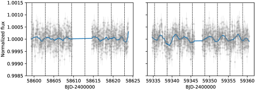
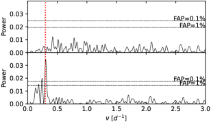
Figure 1: Out-of-transit and out-of-eclipse 30 min cadence TESS photometry of WASP-178 during sector 11 (left panel) and sector 38 (central panel). In each panel, the dashed vertical lines mark the planetary transit, while the solid blue line is a smoothing of the data points to emphasize the correlated noise. The right panel shows the GLS periodogram of sector 11 and 38 (top and bottom box respectively). In each box, we report the bootstrap-computed 0.1% and 1% FAP levels (horizontal dashes) and the planetary orbital period (vertical red dotted line).

The periodicity detected in sector 38 is consistent within uncertainties with the planetary orbital period. Nonetheless, we exclude that this signal is of planetary origin because it remained undetected in sector 11 and is not coherent from orbit to orbit in sector 38. This signal might be due to stellar rotation, and is consistent with the typical amplitude reported by Balona (2011) for A-type stars. Its periodicity would correspond to the $v\sin i_{\star}$ in Table 1 if the inclination of the stellar rotation axis is $\sim 15^{\circ}$. This speculation supports the hypothesis of Rodríguez Martínez et al. (2020) that the star is seen nearly pole-on. A significant misalignment between the stellar rotation axis and the planetary orbit axis is not surprising, both because of its young age (no time for realignment to occur), and the stellar temperature. As a matter of fact, hot stars (T_eff¿6200 K) are observed to often have large misalignments, which is thought to be due to their lack of a convective zone (Winn et al. 2010), needed to tidally align the planetary orbit with the stellar spin axis. Furthermore, Albrecht et al. (2021) found that misaligned orbits are most often polar, or close to polar, as seems to be the case of WASP-178 b. We expand the discussion on the photometric variability and the orientation of the stellar rotation axis in Appendix B.

The fact that the period of the correlated noise is similar to the orbital period of WASP-178 b makes it difficult to extract the complete planetary Phase Curve (PC) signal. We thus first tried a simpler and more robust approach to analyze the planetary transits and eclipses (Sect. 4.1.1), then we attempted a more complex analysis framework aimed at retrieving the full PC of WASP-178 b (Sect. 4.1.2).

4.1.1 Fit of transits and eclipses

We computed the ephemeris of the planet by trimming segments of the LCs centered on the transit events (7 transits in sector 11 and 8 transits in sector 8) and as wide as 3 times the transit duration. To further constrain the ephemeris of WASP-178 b, we included in our analysis the WASP-South photometry (2006 May – 2014 Aug) and EulerCAM I-band photometry (2018 Mar 26) presented in Hellier et al. (2019). Also for the case of the WASP-South photometry, we trimmed the LC around the transits and kept the 24 intervals containing more than 20 data points.

We fit the data using the same Bayesian approach described in Scandariato et al. (2022). In summary, it consists in the fit of a model - in a likelihood-maximization framework - which includes the transits, a linear term for each transit to detrend against stellar/instrumental systematics and a jitter term to fit the white noise not included in the photometric uncertainties. The transit profile is formalized using the quadratic limb darkening (LD) law indicated by Mandel & Agol (2002) with the reparametrization of the LD coefficients suggested by Kipping (2013). For TESS sector 11 the model is rebinned to the same 30 min cadence of the data. The likelihood maximization is performed with MCMC using the python emcee package version 3.1.3 (Foreman-Mackey et al. 2013), using a number of samplings long enough to ensure convergence. We used flat priors for all the fitting parameters but the stellar density, for which we used the Gaussian prior $N(0.43,0.02)$ given by the stellar mass and radius in Table 1. We also used the Gaussian priors for the Limb Darkening (LD) coefficients given by the LDTk package . For simplicity, we use the same LD coefficients for the three datasets. This is motivated by the fact that the WASP-South photometry is not accurate enough to constrain the LD profile, and that the TESS passband is basically centered on the standard I band, thus the same LD profile is expected for the TESS and EulerCAM LCs. Since the model fitting is computationally demanding, we ran the code in the HOTCAT computing infrastructure (Bertocco et al. 2020; Taffoni et al. 2020).

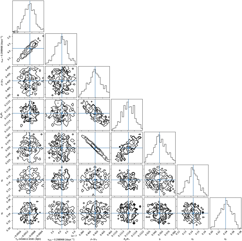
Figure 9: Corner plot of the MCMC chains of planetary parameters from the fit of the TESS transits (see Sect. 4.1.1). In each plot, the solid blue lines mark the MAP values.

The result of the model fitting is listed in Table 3. The orbital solution we derived is consistent with previous studies (Hellier et al. 2019; Rodríguez Martínez et al. 2020) within 5$\sigma$. The best fit model, corresponding to the Maximum A Posteriori (MAP) parameters, is over-plotted to the phase-folded data in Fig 2, where we rebinned the model and the LC of sector 38 to the same 30 min cadence of sector 11 (we do not show the WASP-South and EulerCAM photometry not to clutter the plot). In Fig. 9 we show the corner plot of the system’s parameters from the fit of the transit LCs.

Table 3: Model parameters for the fit of the TESS  WASP-South and EulerCAM data.

Jump parameters	Symbol	Units	MAP	C.I.	Prior
Time of transit	$T_{0}$	BJDTDB-2400000	56612.6581	56612.6581(3)	$U$(56612.6, 56612.7)
Orbital frequency	$\nu_{\rm orb}$	days-1	0.29896856	0.29896855(3)	$U$(0.2989,0.2990)
Stellar density	$\rho_{\star}$	$\rho_{\sun}$	0.45	0.44(1)	$N$(0.43,0.02)
Radii ratio	$R_{p}/R_{\star}$	—	0.1124	0.1125(2)	$U$(0.05,0.12)
Radii ratio	$R_{p}/R_{\star}$	—	0.1109	0.1108(4)	$U$(0.05,0.12)
Radii ratio	$R_{p}/R_{\star}$	—	0.1141	0.1141(4)	$U$(0.05,0.12)
Impact parameter	b	—	0.52	0.51(1)	$U$(0.01,0.9)
First LD coef.	q1	—	0.147	0.147(8)	$N$(0.133,0.014)
Second LD coef.	q2	—	0.344	0.34(2)	$N$(0.333,0.023)
Secondary eclipse depth	$\delta_{\rm ecl}$	ppm	70	70(40)	$U$(0,400)
Derived parameters	Symbol	Units	MAP	C.I.
Planetary radius	Rp	RJ	1.88	1.88(2)	including the stellar radius uncertainty
Planetary radius	Rp	RJ	1.86	1.85(2)	including the stellar radius uncertainty
Planetary radius	Rp	RJ	1.91	1.91(2)	including the stellar radius uncertainty
Orbital period	Porb	day	3.3448332	3.3448333(4)
Transit duration	T14	hr	3.488	3.488(8)
Scaled semi-major axis	$a/R_{\star}$	—	7.20	7.19(6)
Orbital inclination	$i$	degrees	85.8	85.8(1)

Since the TESS LCs of sector 11 and 38 show different levels of variability, we investigated any seasonal dependence of the apparent planet-to-star radius ratio. We used the same Bayesian framework as above, where we fix the ephemeris of WASP-178. The planet-to-star radius ratio we derived is 0.1108$\pm$0.0004 for sector 11 and 0.1141$\pm$0.0004 for sector 38. The difference is thus 0.0033$\pm$0.0006, that is we found different transit depths with a 5.5$\sigma$ significance. In particular, we remark that the planet looks larger in sector 38, where the rotation signal is stronger. We thus speculate that WASP-178 was in a low variability state during sector 11, while one year later ($\sim$80 stellar rotations) during sector 38 the stellar surface hosted dark spots in co-rotation with the star. This hypothesis is consistent with Hümmerich et al. (2018), according to which magnetic chemically peculiar stars may show complex photometric patterns due to surface inhomogeneities.

We used a similar framework to extract the secondary eclipse signal of WASP-178: we simultaneously fit segments of the TESS LCs centered on the planetary eclipses keeping fixed the ephemeris of WASP-178 to the values listed in Table 3. We did not attempt the disjoint analysis of the two sectors as the expected eclipse depth is of the order of $\sim$100 ppm (see below), and the photometric precision of the LCs is not good enough to appreciate differences in the eclipse depth with enough statistical evidence. The only free planetary parameter of the model is thus the eclipse depth, which turned out to be $\delta_{\rm ecl}=70\pm 40$ ppm (MAP: 70 ppm). The detrended phase-folded eclipses are shown in Fig 2 together with the MAP model.

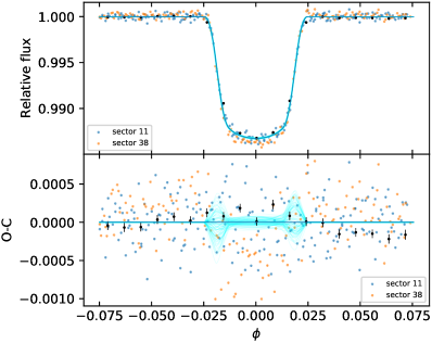
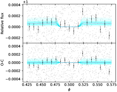
Figure 2: Best fit of the transits and eclipses observed by TESS. Left - Detrended and phase-folded planetary transits (top panel). The photometry of sector 11 and 38 are shown with different colors to emphasize the difference in transit depth (the photometry of sectors 11 and 38 is systematically offset respectively upwards and downwards with respect to the bestfit transit profile). The solid blue line is the best fit model, while the cyan lines represent 100 models corresponding to random samples of the MCMC fit. For the sake of comparison, the photometry of sector 38 and the theoretical models are rebinned to the same 30 min cadence of sector 11. The black dots represent the rebinned photometry. The corresponding O-C diagram is shown in the bottom panel. Right - Same as in the left panel, but centered on the eclipse. For clarity, we do not mark the two sectors with different colors.

4.1.2 Fit of the phase curve

As a more advanced data analysis, we jointly fit the two TESS sectors to extract the full planetary PC (for a homogeneous analysis, we rebinned sector 38 to the same 30 min cadence of sector 11). The fitting model now includes the transits, secondary eclipses, the planetary PC, a Gaussian Process (GP) to fit the correlated noise in the data and, for each TESS sector, a long-term linear trend and a jitter term. Given the system parameters listed in Table 1, the expected amplitude of ellipsoidal variations (Morris 1985) and Doppler boosting (Barclay et al. 2012) in the planetary PC are 2.5 ppm and 1 ppm respectively, out of reach for the TESS photometry. Hence, for the sake of simplicity, we do not include them in the model fitting.

We jointly fit the two TESS sectors, starting with the simplest model where the out of transit PC is flat (that is, we assumed that the planetary PC is not detectable) and the putative stellar rotation is modeled as GP with the SHO kernel, indicated for quasi-periodic signals. Checking the residuals of the fit we notice that some aperiodic correlated noise is left. We thus increased the complexity of the GP model by adding a Matérn3/2 kernel to capture the remaining correlated noise adding only two free parameters to the model. This composite GP model turned out to ensure better convergence to the fit of the model.

Finally, we also included the planetary PC. Assuming that the planet is basically composed of two homogeneous dayside and nightside, the PC is in principle the combination of three components: the PC due to reflected light (with amplitude $A_{\rm refl}$), the PC of the planetary night side (with amplitude $A_{\rm n}$) and the PC of the planetary day side, whose amplitude $A_{\rm d}$ is parameterized such to be larger than $A_{\rm n}$ by an increment $\delta_{\rm d}$ (this parametrization avoids the nonphysical case of a planetary night side brighter than the dayside). The three terms are modeled assuming Lambert’s cosine law.

For the reflected PC, the amplitude can be expressed as:

$$A_{\rm refl}=A_{\rm g}\left(\frac{R_{\rm p}}{a}\right)^{2},$$ (1)

where $A_{\rm g}$ is the planetary geometric albedo (Seager 2010). Assuming a Lambertian reflective planetary surface, the geometric albedo is fixed by the Bond albedo $A_{\rm B}$ by $A_{\rm g}$=$\frac{2}{3}A_{\rm B}$. In the optimistic case of a perfectly reflecting body ($A_{\rm B}$=1), the maximum amplitude for the reflected PC is thus $A_{\rm refl}=167\pm 5$ ppm, where we have used the system parameters in Table 3.

With a slight re-adaptation of the formalism in Seager (2010), the amplitude thermal component $A_{\rm therm}$ can be expressed as:

$$A_{\rm therm}=\left(\frac{R_{\rm p}}{R_{\star}}\right)^{2}\frac{\int\eta(\lambda)B(\lambda,T)d\lambda}{\int\eta(\lambda)I_{\star}(\lambda,T_{\rm eff})d\lambda},$$ (2)

where $\eta(\lambda)$ is the optical throughput of the telescope and $I_{\star}(\lambda,T_{\rm eff})$ is the expected stellar intensity computed with the NextGen model (Hauschildt et al. 1999) corresponding to the effective temperature $T_{\rm eff}$. For the planetary thermal emission we lack the infrared information which can constrain the emission spectrum. We thus assume a black body spectrum $B(\lambda,T)$ at temperature $T$.

The amplitude of the thermal emission from the dayside and the nightside depends on the respective temperatures, which we estimated following Cowan & Agol (2011). The expected temperature of the substellar point of WASP-178 b is:

$$T_{\rm 0}=T_{\rm eff}\sqrt{\frac{R_{\star}}{a}}=3530\pm 60\leavevmode\nobreak\ {\rm K},$$ (3)

where we used the stellar effective temperature in Table 1 and the scaled semi-major axis in Table 3.

The nightside temperature $T_{\rm n}$ and the dayside temperature $T_{\rm d}$ depend on the Bond albedo $A_{B}$ and heat recirculation coefficient $\epsilon$:

$$T_{\rm n} =T_{\rm 0}\left(1-A_{\rm B}\right)^{1/4}\left(\frac{\epsilon}{4}\right)^{1/4}$$ (4)

$$T_{\rm d} =T_{\rm 0}\left(1-A_{\rm B}\right)^{1/4}\left(\frac{2}{3}-\frac{5}{12}\epsilon\right)^{1/4}$$ (5)

The highest dayside temperature, corresponding to $A_{\rm B}$=0 and no heat recirculation ($\epsilon=0$), is:

$$T_{\rm d}=T_{\rm 0}\left(\frac{2}{3}\right)^{1/4}=3190\pm 60\leavevmode\nobreak\ {\rm K},$$ (6)

while the maximum nightside temperature, obtained in the case of full energy recirculation ($\epsilon=1$), is:

$$T_{\rm n}=T_{\rm 0}\left(\frac{1}{4}\right)^{1/4}=2500\pm 40\leavevmode\nobreak\ {\rm K}.$$ (7)

These maximum temperatures lead to the upper limit on the dayside ($A_{\rm d}$) and nightside ($A_{\rm n}$) thermal emission amplitude of:

$$A_{\rm d}=225\pm 27\leavevmode\nobreak\ {\rm ppm};A_{\rm n}=48\pm 7\leavevmode\nobreak\ {\rm ppm}.$$ (8)

In Fig. 3 we plot the upper limits for the three PCs discussed so far. The figure shows that the three components may reach amplitudes of comparable orders of magnitude, meaning that none of them can in principle be neglected in the extraction of the planetary PC. We note that the two components belonging to the dayside (reflection and thermal emission) have the same shape, thus it is not possible to disentangle them. To simplify the model and avoid the degeneracy between dayside reflection and emission, we thus artificially set $A_{\rm refl}=0$ and let $A_{\rm d}$ absorb the whole signal belonging to the planetary dayside.

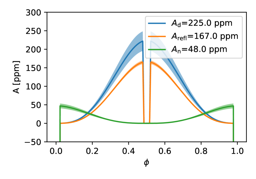
Figure 3: Upper limits on the reflected PC, dayside thermal PC and nightside thermal PC for WASP-178 b.

The Akaike Information Criterion (AIC, Burnham & Anderson 2002) favors the model that includes the planetary PCs. The simpler model with flat out-of-transit PC has a relative likelihood of 55% and cannot be rejected. The posterior distributions of the common parameters (system ephemeris and planet-to-star radii ratio) between the two models do not differ significantly.

For both models, the SHO GP has a frequency $\nu\sim$0.30 d^-1, an amplitude $\sim$70 ppm and a timescale $\sim$11 d. Frequency $\nu$ and the amplitude of the quasi-periodic GP are consistent with the frequency and amplitude of the periodic signal found in the periodogram (Sect. 4.1). While the correspondence between the orbital period of WASP-178 b and the periodicity of the GP suggests that the red noise in the data is of planetary origin, we do not have other strong evidence that support this hypothesis. On the contrary, the planetary origin seems odd for the reasons discussed in Sect. 4.1. The aperiodic red noise fitted as a Matérn3/2 GP has an amplitude $\sim$150 ppm and a timescale of $\sim$50 min. Despite the aperiodic red noise evolves on timescales shorter than the transit duration ($T_{\rm 14}$=3.53 hr), the retrieved posterior distributions of the orbital parameters are similar to the ones obtained in Sect. 4.1.1.

Regarding the retrieval of the planetary PCs, we derived an upper limit of $A_{\rm n}<$174 ppm at the 99.9% confidence level, while for the dayside we derived a 1$\sigma$ confidence band of 110$\pm$40 ppm which includes both the reflection and thermal emission components. We remark that the $A_{\rm d}$ parameter corresponds in our model to the eclipse depth $\delta_{\rm ecl}$ and is consistent within uncertainties with the estimate reported in Table 3.

The fit of the full TESS LC thus confirms the results previously obtained in Sect. 4.1.1. Given the similarities between the results obtained with the two approaches, we preferred the former one as it is less prone to interference between the data detrending and the extraction of the orbital parameters and the eclipse depth.

4.2 CHEOPS photometry

To analyze the CHEOPS LCs we use the same approach as for the fit of the eclipses observed by TESS (Sect. 4.1.1), with an additional module in the fitting model that takes into account the systematics in the CHEOPS data. As a matter of fact, CHEOPS photometry is affected by variable contamination from background stars in the field of view (e.g. Lendl et al. 2020; Deline et al. 2022; Hooton et al. 2022; Wilson et al. 2022; Scandariato et al. 2022). This variability is due to the interplay of the asymmetric PSF with the rotation of the field of view (Benz et al. 2021). PIPE by design uses nominal magnitudes and coordinates of the stars in the field to fit the stellar PSFs, but residual correlated noise is present in the LCs due to inaccuracies in the assumptions. This signal is phased with the roll angle of the CHEOPS satellite and, in the case of WASP-178, is clearly visible in the GLS periodogram of the data together with its harmonics. To remove this signal, we included in our algorithm a module which fits independently for each visit the harmonic expansions of the telecope’s orbital period and its harmonics. A posteriori, we found that the roll angle phased modulation is adequately suppressed (that is, there is no peak in the periodograms at the frequencies in the harmonic series) if we include in the model the fundamental harmonic and its first two harmonics.

We also noticed that the photometry is significantly correlated with the coordinates of the centroid of the PSF on the detector. To decorrelate against this instrumental jitter we thus included in the model a bi-linear function of the centroid coordinates.

Finally, to take into account a white noise not included in the formal photometric uncertainties, we add to our model a diagonal GP kernel of the form:

$$k(t_{i},t_{j})=j_{v}^{2}\delta_{i,j},$$ (9)

with an independent jitter term $j_{v}$ for each CHEOPS visit.

As for the fit of the TESS data (Sect. 4.1.1), we search the bestfit parameters through likelihood-maximization in a MCMC framework, and we find $\rm\delta_{ecl}=70\pm 20$ ppm. The ephemeris of the planet were locked to the MAP values listed in Table 3, which guarantee an uncertainty on the eclipse time less than 23 s for each CHEOPS visit. The phase-folded data detrended against stellar and instrumental correlated noise are shown in Fig. 4.

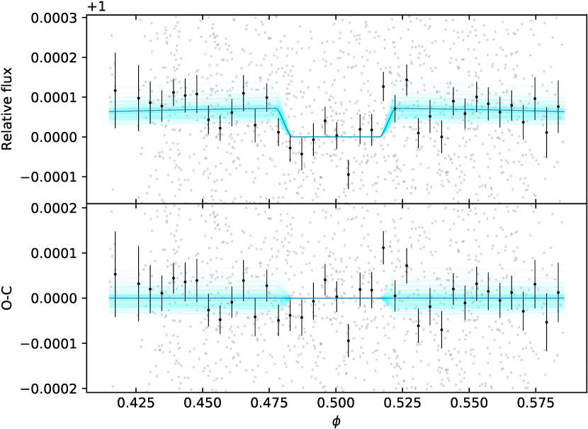
Figure 4: Same as the right panel in Fig. 2 for the eclipses of WASP-178 observed by CHEOPS.

5 Discussion

In the previous sections we have analyzed the TESS and CHEOPS PCs of WASP-178 b in order to extract its planetary eclipse depth $\delta_{\rm ecl}$, obtaining respectively $70\pm 40$ ppm and $70\pm 20$ ppm. These two measurements take into account both the reflection from the planetary dayside and its thermal emission. With the assumptions discussed below, the combined information on the eclipse depth from two different instruments allows to disentangle these two contributions. For a given telescope with passband $\eta(\lambda)$ we can combine Eq. 1 and Eq. 2 obtaining:

$$\delta_{\rm ecl}=A_{\rm g}\left(\frac{R_{\rm p}}{a}\right)^{2}+\left(\frac{R_{\rm p}}{R_{\star}}\right)^{2}\frac{\int\eta(\lambda)B(\lambda,T_{\rm d})d\lambda}{\int\eta(\lambda)I_{\star}(\lambda,T_{\rm eff})d\lambda},$$ (10)

where $T_{\rm d}$ is the planetary dayside temperature.

Solving for $A_{\rm g}$, and indicating with the subscripts $C$ (for CHEOPS) and $T$ (for TESS) the wavelength-dependent quantities, we obtain:

$$\begin{cases}A_{\rm g}^{C}=\left(\frac{a}{R_{\star}}\right)^{2}\left[\frac{\delta_{\rm ecl}^{C}}{\left(\frac{R_{\rm p}}{R_{\star}}\right)^{2}}-\frac{\int\eta^{C}(\lambda)B(\lambda,T_{\rm d})d\lambda}{\int\eta^{C}(\lambda)I_{\star}(\lambda,T_{\rm eff})d\lambda}\right],\\ A_{\rm g}^{T}=\left(\frac{a}{R_{\star}}\right)^{2}\left[\frac{\delta_{\rm ecl}^{T}}{\left(\frac{R_{\rm p}}{R_{\star}}\right)^{2}}-\frac{\int\eta^{T}(\lambda)B(\lambda,T_{\rm d})d\lambda}{\int\eta^{T}(\lambda)I_{\star}(\lambda,T_{\rm eff})d\lambda}\right].\end{cases}$$ (11)

In the most general case, $A_{g}^{C}$ and $A_{g}^{T}$ differ according to the planetary reflection spectrum. Since we do not have any spectroscopic analysis of the dayside of WASP-178 b, we define the proportionality coefficient $\alpha=A_{g}^{T}/A_{g}^{C}$ to account for differences between the two passbands. Solving Eq. 11 for $T_{\rm d}$ we thus obtain the implicit function:

$$\frac{\alpha\delta_{\rm ecl}^{C}-\delta_{\rm ecl}^{T}}{\left(\frac{R_{\rm p}}{R_{\star}}\right)^{2}}+\frac{\int\eta^{T}(\lambda)B(\lambda,T_{\rm d})d\lambda}{\int\eta^{T}(\lambda)I_{\star}(\lambda)d\lambda}-\alpha\frac{\int\eta^{C}(\lambda)B(\lambda,T_{\rm d})d\lambda}{\int\eta^{C}(\lambda)I_{\star}(\lambda)d\lambda}=0.$$ (12)

We initially assumed the simplest scenario of a gray albedo spectrum ($\alpha$=1) in the spectral range covered by CHEOPS and TESS (the respective bandpasses are shown in Fig. 6). In this scenario, we expect that the contribution of reflection to the eclipse depth is the same in the CHEOPS and TESS passbands. We also expect that the thermal emission from a $T\simeq$3000 K black body has a larger contribution in the TESS passband, because it favors redder wavelengths compared with CHEOPS (see Fig. 6).

To estimate the dayside temperature $T_{\rm d}$ that best explains our best observations together with its corresponding uncertainty, we randomly extracted 10 000 steps from the Monte Carlo chains obtained in the fit of the transit and eclipse LCs (Sect. 4.1.1 and 4.2). We also generated 10 000 samples of the stellar effective temperature using a normal distribution with mean and standard deviations as reported in Table 1. For each of the 10 000 samples we thus numerically solved Eq. 12 using the fsolve method of the scipy Python package, thus obtaining 10 000 samples of $T_{\rm d}$. Then, we plugged all the samples back into Eq. 11 to derive $A_{g}^{C}$(=$A_{g}^{T}$).

The root finding algorithm failed for $\sim$50% of the samples. These failures correspond to the combination of parameters that prevent Eq. 12 from having a $T_{\rm d}$ root in the domain of real numbers. This happens in particular for the samples where $\delta_{\rm ecl}^{T}<\delta_{\rm ecl}^{C}$ that, as discussed above, are not consistent with the gray albedo hypothesis. We thus reject these samples and show in Fig. 7 the $A_{g}^{C}$–$T_{\rm d}$ density map of the remaining ones. Our results indicate $A_{g}^{C}=0.2\pm 0.1$ and $T_{\rm d}=2400\pm 300$ K, consistent with the temperature-pressure profile derived by (Lothringer et al. 2022) at pressure higher that 1$\rm\mu$bar by means of ultraviolet transmission spectroscopy. Our result also follows the general trend of $A_{\rm g}$ increasing with $T_{\rm d}$ indicated by Wong et al. (2021) (Fig. 5).

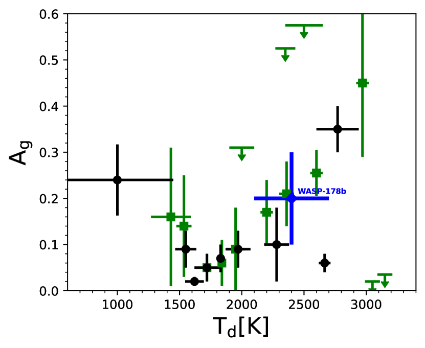
Figure 5: Adaptation of Fig. 10 in Wong et al. (2021) including our analysis of WASP-178 b (in blue). The green squares indicate the systems from the first and second year of the TESS primary mission. The black circles indicate the Kepler-/CoRoT-band geometric albedos for the targets that were observed by those missions.

By definition, the geometric albedo $A_{\rm g}$ refers to the incident light reflected back to the star at a given wavelength (or bandpass). Integrating at all angles, the spherical albedo $A_{\rm S}$ is related to $A_{\rm g}$ by the phase integral $q$: $A_{\rm S}$=$q$$A_{\rm g}$ (see for example Seager 2010). Depending on the scattering law, exoplanetary atmospheres have 1¡$q$¡1.5 (Pollack et al. 1986; Burrows & Orton 2010). Unfortunately, for the reasons explained in Sect. 4.1.2, we could not extract a robust phase curve for WASP-178 b, hence we could not place any better constraint on $q$. In the following we thus consider the two limiting scenarios $A_{S}^{\rm min}=A_{g}$ and $A_{S}^{\rm max}=1.5A_{g}$.

The Bond albedo $A_{\rm B}$ is computed as the average of $A_{\rm S}$ weighted over the incident stellar spectrum:

$$A_{\rm B}=\frac{\int_{0}^{\infty}A_{\rm S}(\lambda)I_{\star}(\lambda)d\lambda}{\int_{0}^{\infty}I_{\star}(\lambda)d\lambda}.$$ (13)

The conversion into $A_{\rm B}$ thus relies on the measurement of $A_{\rm S}$ across the stellar spectrum. In this study we only covered the optical and near-infrared part of the spectrum, as shown in Fig. 6, and we lack the necessary information in the UV, mid, and far infrared domains. Following the approach of Schwartz & Cowan (2015), we explore the scenario of minimum Bond albedo $A_{\rm B}^{\rm min}$ obtained through Eq. 13 assuming $A_{\rm S}$=$A_{\rm S}^{\rm min}$ in the spectral range covered by CHEOPS and TESS and $A_{\rm S}$=0 otherwise. The opposite limiting case assumes $A_{\rm S}$$(\lambda)=A_{\rm S}^{\rm max}$ at all wavelength, which leads to $A_{\rm B}^{\rm max}=A_{\rm S}^{\rm max}$. To compute the integrals in Eq. 13, we used the synthetic spectrum in the BT-Settl library corresponding to the parameters of WASP-178 (Allard et al. 2012).

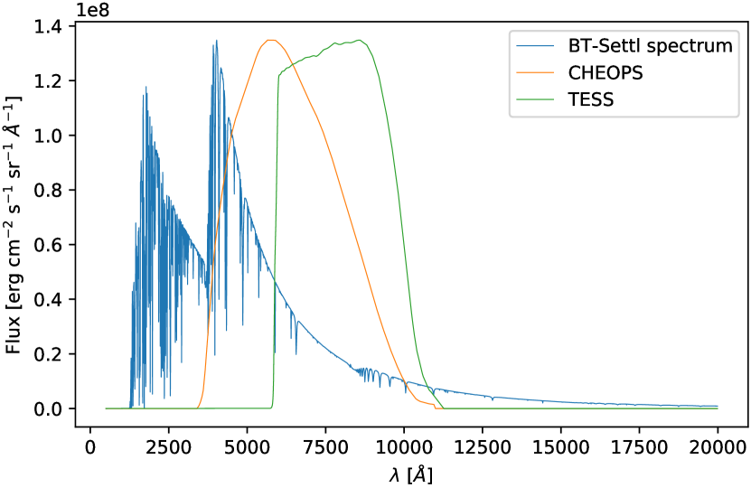
Figure 6: BT-Settl synthetic stellar spectrum for WASP-178 together with the CHEOPS and TESS passbands.

Under the hypothesis that $\alpha=1$, we obtained samples of $A_{\rm g}^{C}=A_{\rm g}^{T}=$$A_{\rm g}$, which now translate into samples of $A_{\rm B}^{\rm min}$ and $A_{\rm B}^{\rm max}$ with the assumptions discussed above. Moreover, inverting Eq. 5 yields to:

$$\epsilon=\frac{1}{5}\left[8-\left(\frac{T_{\rm d}}{T_{\rm eff}}\right)^{4}\left(\frac{a}{R_{\star}}\right)^{2}\frac{12}{1-A_{\rm B}}\right].$$ (14)

Equation 14 indicates that $\epsilon$ is a decreasing function of $A_{\rm B}$. Plugging in the samples of $T_{\rm d}$, T_eff, $a/R_{\star}$ and alternatively $A_{\rm B}^{\rm min}$ and $A_{\rm B}^{\rm max}$, we obtained the corresponding samples $\epsilon^{\rm max}$ and $\epsilon^{\rm min}$.

The albedo–recirculation density maps of the two scenarios are shown in the right panel of Fig. 7. Unsurprisingly, we find that the upper limit on $A_{\rm B}$ is larger ($\sim$0.6) in the scenario where all the factors concur to push up the reflectivity of the atmosphere (high $q$ and maximum $A_{\rm S}$), and it decreases to $\sim$0.3 in the opposite scenario of minimum reflectivity.

The recirculation coefficient $\epsilon$ tends towards large values, eventually exceeding 1 due to measurement uncertainties, in both scenarios. While $\epsilon>1$ is physically meaningless, still the posterior distribution indicates a high level of atmospheric energy recirculation in both cases of minimum and maximum albedo ($\epsilon^{\rm max}=1.0\pm 0.3$ and $\epsilon^{\rm min}=0.8\pm 0.3$ respectively). Following different atmospheric models (e.g., Perez-Becker & Showman 2013; Komacek & Showman 2016; Schwartz et al. 2017; Parmentier & Crossfield 2018), WASP-178 b is in a temperature regime where heat recirculation of zonal winds is suppressed and recirculation efficiency is expected to be low. Nonetheless, Zhang et al. (2018) collected observational evidence that Hot Jupiters with irradiation temperatures similar to the one of WASP-178 b are characterized by efficient day-to-night recirculation. Using the global circulation models of Kataria et al. (2016), they ascribed this efficiency to the presence of zonal winds, that also explain the eastward offset of the PC of the same planets. While the theoretical predictions on the offset (and the recirculation efficiency correspondingly) likely overestimate the truth (see Fig. 15 in Zhang et al. 2018), still there is an indication that zonal winds might indeed explain the energy transfer from the dayside to the nightside of WASP-178 b.

Unfortunately, as discussed in Sect.4.1.2, it is difficult to disentangle the planetary phase curve and the stellar variability. By consequence, any measurement of the phase curve offset is precluded. Another possibility is that ionized winds flow from the dayside, where temperatures higher that 2500 K leads to complete dissociation of H₂, to the nightside, where lower temperatures allow the molecular recombination and the consequent energy release. This scenario is supported by several recent studies (Bell & Cowan 2018; Tan & Komacek 2019; Mansfield et al. 2020; Helling et al. 2021, 2023).

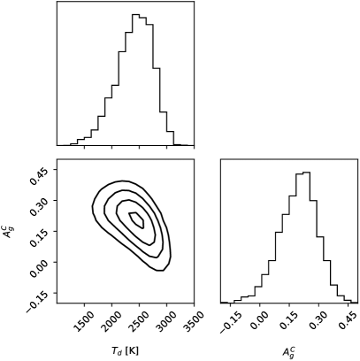
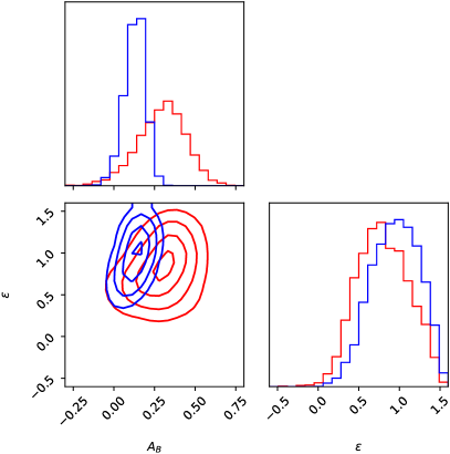
Figure 7: Left panel - $A_{g}^{C}$–$T_{\rm d}$ density maps in the case of $\alpha=1$. Right panel - Albedo–recirculation density maps assuming maximum $A_{\rm B}$ (red contours) and minimum $A_{\rm B}$ (blue contours).

According to the synthetic models computed by Sudarsky et al. (2000), the albedo spectrum of highly irradiated giant planets is expected to show molecular absorption bands by H₂O at around 1 $\mu m$ and longer wavelength. Since the passband of TESS is more sensitive in the near-infrared than CHEOPS, it is plausible to assume that the geometric albedo in the TESS passband is lower than for CHEOPS. In order to assess how the assumption on $\alpha$ affects our results, we re-run our analysis assuming an extreme $\alpha=0.5$. The results are shown in Fig. 8: we find almost the same posterior distribution for dayside temperature, albedo and recirculation, indicating that the most important source of uncertainties are not the assumptions we make but the measurement uncertainties on the eclipse depth extracted from the CHEOPS and TESS LCs.

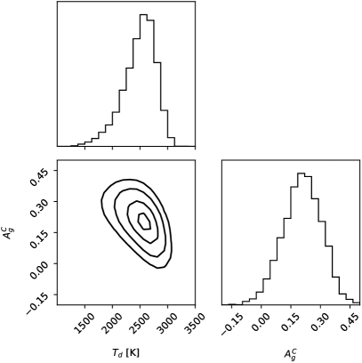
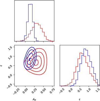
Figure 8: Same as in Fig. 7 in the case $\alpha=0.5$.

6 Summary and conclusion

In this work we have analyzed the space-borne photometry of the WASP-178 system obtained with TESS and CHEOPS. For both telescopes we have tailored the photometric extraction in order to avoid the strong contamination by a background eclipsing binary. We have found evidence that the stellar host is rotating with a period of $\sim$3 days, consistent with the orbital period of its HJ, and that it is seen in a pole-on geometry.

The similarity between the stellar rotation period and the orbital period of the planet, coupled with the quality of the TESS data, does not allow a robust analysis of the full PC of the planet, nor we could put strong constraints on the planetary nightside emission. Nonetheless, focusing on the transit and eclipse events, we could update the ephemeris of the planet and measure an eclipse depth of 70$\pm$40 ppm and 70$\pm$20 ppm in the TESS and CHEOPS passband respectively.

The joint analysis of the eclipse depth measured in the two passbands allowed us to constrain the temperature in the 2250–2750 K range, consistent with the temperature-pressure profile derived by (Lothringer et al. 2022) at pressure higher that 1$\rm\mu$bar. Moreover, we could also constrain the optical geometric albedo $A_{\rm g}$¡0.4, which fits the general increasing albedo with stellar irradiation indicated by Wong et al. (2021).

Finally, we found indication of an efficient atmospheric heat recirculation of WASP-178 b. If confirmed, this evidence challenges the models that predict a decreasing heat transport by zonal winds as the equilibrium temperature increases (e.g., Perez-Becker & Showman 2013; Komacek & Showman 2016; Schwartz et al. 2017; Parmentier & Crossfield 2018). Conversely, WASP-178 b is an interesting target to test atmospheric models where heat transport is granted by ionized winds from the dayside to the nightside, where the recombination of H₂ takes place (e.g. Mansfield et al. 2020; Helling et al. 2021, 2023). Additional observations of WASP-178 b are needed to better constrain its atmospheric recirculation and rank current competing models. The WASP-178 system is going to be observed again by TESS in May 2023, but this is not expected to add much to the two sectors analyzed in this work. Conversely, dedicated observations from larger space observatories might provide helpful insights of the physical and chemical equilibrium of the atmosphere of WASP-178 b.

Appendix A Posterior distributions of the model parameters from the fit of the TESS transit light curves

Appendix B Analysis of the TESS transits in high cadence

In Sect. 4.1 we analyzed the TESS photometry at low cadence (30 min), and we found a significant difference between the transit depth between sectors 11 and 38. We speculated that the difference in transit depth is due to photospheric variability, which manifests also as a quasi-periodic signal in the LC of sector 38. This hypothesis is supported by the growing evidence that A-type stars show rotational signals due to photospheric inhomogeneities (e.g., Balona 2011; Böhm et al. 2015; Sikora et al. 2020). This scenario is further supported by the fact that the WASP-178 is classified as an Am star by Hellier et al. (2019).

To test if the visible hemisphere of the star hosts dark spots, we searched for transit anomalies in the TESS LCs, that are localized bumps in the residuals of the transit fits. If present, they indicate that the planet’s projection on the stellar surface crosses a darker area compared to the quiescent photosphere (see for example Béky et al. 2014; Scandariato et al. 2017). To this purpose, the low cadence photometry analyzed in Sect. 4.1 is of little help, as a finer time sampling is needed. We thus compared the high cadence (2 min) TESS photometry of sector 38 with the bestfit model discussed in Sect. 4.1.2, computed using $R_{\rm p}/R*$=0.1141 (see Sect. 4.1.1). This comparison does not show any bump inside the transits (Figs. 10–13), and we concluded that in the eight transits observed in sector 38 there is no spot-crossing event.

We also remark that, in contrast with Rodríguez Martínez et al. (2020), we did not detect any systematic asymmetry in the transit profile. The stellar flux distribution along the transit path is symmetric with respect to the transit center. This either indicates that the star does not show any gravity darkening, which is unlikely if the stellar rotation period of $\sim$3.2 days is confirmed, or supports the hypothesis that the star is in a pole-on geometry, which leads to a radially symmetric flux distribution over the visible stellar hemisphere.

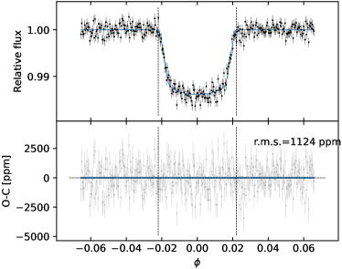
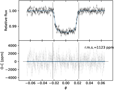
Figure 10: Detrended short cadence LC of the first (left panel) and second (right panel) transit observed in TESS sector 38. In each panel, the top plot shows the model computed with the MAP parameters in Table 3 as a blue solid line. The bottom plots show the residuals of the short cadence photometry with respect to the planetary model shown in the top panel. As a guide, we plot with a blue line the smoothing of the residuals obtained with a Savitzky-Golay filter. In all plots, the vertical dashed lines mark the first and fourth contacts.

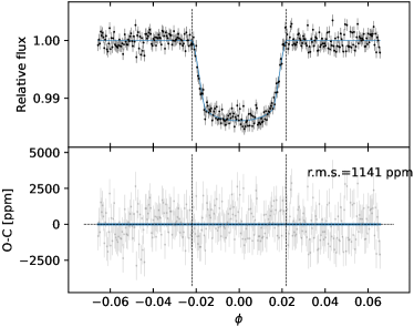
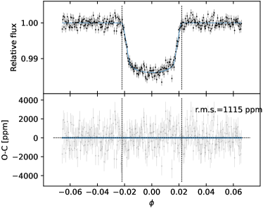
Figure 11: Detrended short cadence LC of the third (left panel) and fourth (right panel) transit observed in TESS sector 38. Details are the same as in Fig. 10.

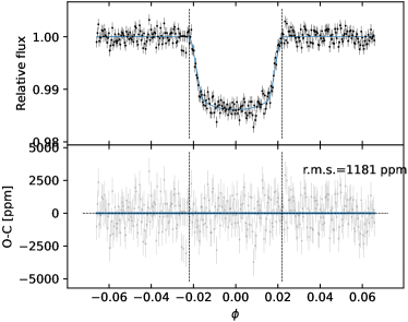
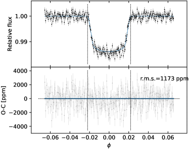
Figure 12: Detrended short cadence LC of the fifth (left panel) and sixth (right panel) transit observed in TESS sector 38. Details are the same as in Fig. 10.

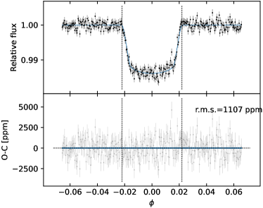
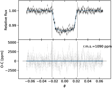
Figure 13: Detrended short cadence LC of the seventh (left panel) and eighth (right panel) transit observed in TESS sector 38. Details are the same as in Fig. 10.