Microscale 3-D Capacitance Tomography with a CMOS Sensor Array

Abstract

Electrical capacitance tomography (ECT) is a non-optical imaging technique in which a map of the interior permittivity of a volume is estimated by making capacitance measurements at its boundary and solving an inverse problem. While previous ECT demonstrations have often been at centimeter scales, ECT is not limited to macroscopic systems. In this paper, we demonstrate ECT imaging of polymer microspheres and bacterial biofilms using a CMOS microelectrode array, achieving spatial resolution of 10 microns. Additionally, we propose a deep learning architecture and an improved multi-objective training scheme for reconstructing out-of-plane permittivity maps from the sensor measurements. Experimental results show that the proposed approach is able to resolve microscopic 3-D structures, achieving 91.5% prediction accuracy on the microsphere dataset and 82.7% on the biofilm dataset, including an average of 4.6% improvement over baseline computational methods.

I Introduction

Electrical capacitance tomography (ECT) is an imaging technique that estimates the internal distribution of permittivity in a volume by measuring capacitance between electrodes placed at its boundary [16]. It is closely related to electrical impedance tomography (EIT), which estimates the conductivity distribution using impedance measurements [7]. Both of these techniques are useful in applications where there is spatial contrast in conductivity or permittivity, including organ and tissue imaging [1, 25, 8, 30, 31], neural imaging and neural activity monitoring [3, 4], [29], and industrial process monitoring of fluid flows [17], [23].

The physics of the ECT problem, in 2-D, are managed by the Poisson PDE in Eq. 1, where $\sigma(x,y)$ represents the permittivity distribution and $u(x,y)$ represents the electric potential [2]. Mutual capacitance $C_{ij}$ between electrodes $i$, $j$ is evaluated by the integral in Eq. 2, where $V_{ij}$ is the potential difference between the two electrodes, and $S$ is the path enclosing the sensing electrodes. The problem of estimating the capacitance given the permittivity distribution is referred to as the forward problem [10]. Conversely, estimating the permittivity distribution from boundary capacitance measurements is referred to as the inverse problem.

$$\nabla.(\sigma(x,y)\nabla u(x,y))=0\vspace*{-2mm}$$ (1)

$$C_{ij}=-\frac{Q}{V_{ij}}=-\frac{\oint_{s}\sigma(x,y)\nabla u(x,y)ds}{u_{i}-u_{j}}\vspace*{-0.5mm}$$ (2)

The inverse problem of ECT is a non-linear and severely ill-posed problem, without unique numerical solutions[33]. Therefore, regularization priors are often used to impose an additional constraint on the estimated solution [22]. Traditional algorithms solve the inverse problem by minimizing a least squares objective with an additional regularization term for an initial permittivity distribution through an iterative solver  [33, 34, 5]. However, iterative algorithms are sensitive to noise in the capacitance measurements which makes them more susceptible to divergence. Prior work demonstrates that deep learning models can be more robust to experimental noise and can provide accurate image reconstructions [37], [38], [39], [32].

Previous demonstrations of ECT have often resolved centimeter-scale targets. If it could be appropriately miniaturized, one appealing application of ECT would be for 3-D visualization of cell cultures [19, 24, 12]. Optical confocal microscopy is a powerful tool for biologists to image the 3-D structure of complex cell cultures [26]. However, confocal imaging can be prohibitively expensive for routine use, usually relies on fluorescent labeling, and its intense light excitation introduces tradeoffs between the frame rate and risks of photobleaching and phototoxicity.

Here we propose a microscale capacitance tomography system using a 512 $\times$ 256 CMOS sensor array [15, 14, 13], achieving the highest-resolution ECT reported to date (10 $\mu$m). We apply deep learning to approximate the ECT inverse operator, using training data as a regularization prior to the ill-posed inverse problem. The proposed system enables imaging of micro 3-D structures of cell cultures with a high reconstruction accuracy. We present results for two experimental datasets of microscopic objects: polymer microspheres and bacterial biofilms. The ECT data are trained and evaluated using ground truth images acquired from 3-D confocal microscopy.

Figure 1: Overview of the tomography system. (a) Illustration of the one-sided planar ECT detection using the CMOS sensor. The sample, above the sensor, has a permittivity value $\varepsilon_{1}$ distinct from the background permittivity $\varepsilon_{0}$. (b) Image reconstruction network, based on transposed convolution. The input is a matrix of pairwise capacitance measurements acquired from the CMOS sensor. The output is a $100$ $\times$ $200\,\mu m$ cross-sectional image that represents the permittivity distribution $\sigma(z,y)$.

II Methodology

II-A Capacitance Tomography Hardware

The tomography is implemented using measurements from an integrated CMOS microelectrode array described in [15]. This chip has a 512 $\times$ 256 planar array of microelectrodes on a 10 $\mu$m $\times$ 10 $\mu$m rectangular grid. In one of its operating modes, the chip can efficiently measure the mutual capacitance between any two pixels in the array [14, 13]. Fig. 1(a) illustrates the one-sided planar detection using the sensor, where electrodes are only placed at the bottom boundary. Each capacitance $C_{ij}$ represents fringing electric fields through the sample, and thus the permittivity and geometry of materials near the sensor influence these measurements. Samples to be imaged are placed on the chip surface in a liquid or gel electrolyte, as illustrated in Fig. 3(a). An image of the sensor is shown in Fig. 3(b).

II-B Image Reconstruction Network

Fig. 1(b) illustrates the architecture of the image reconstruction network. The input is an $m\times n$ matrix containing pairwise capacitance measurements, where $m$ is the number of spatial offsets considered when measuring the mutual capacitance values and $n$ is the number of electrodes. Each entry in the matrix corresponds to the mutual capacitance $C_{ij}$ between electrodes $i$ and $j$. For example, the first row contains $n$ capacitance values measured between adjacent electrodes, and the second row contains measurements between electrodes separated by $2$ positions. In this study, we only use capacitance measurements with $|i-j|\leq 5$. To make the input matrix compatible with the transposed convolution layer, we reshape it to a 3-D feature map of size $(w,h,c)=(1,1,\textrm{num\_measurements})$. The input 3-D feature map is then repeatedly up-sampled by a factor of $2$ until it reaches the spatial resolution of the predicted cross-sectional image $(w,h,c)=(200,100,1)$, which represents the permittivity distribution $\sigma(z,y)$ of the medium above the CMOS sensor.

The boundary capacitance measurements are up-sampled through a series of five transposed convolution blocks. Each block contains a transposed convolution layer, batch normalization layer, and a ReLU activation, except for the last block where sigmoid activation is used to constrain the output permittivity to be in the range $[0,1]$. The transposed convolution layer contains a learnable kernel that is used to reconstruct a high-resolution output from a low-resolution input [9]. Batch normalization is used for training stability and convergence speed-up. Additionally, a residual connection is added between the block input and output through a $1\text{x}1$ convolution kernel.

II-C Loss

The loss function is important in training deep learning algorithms as it defines the optimization landscape and has a significant impact on the model convergence [35]. Class imbalance, where the foreground permittivity occupies a significantly smaller region relative to the background pixels, poses a challenge in training. As noted by [39], distribution-based loss functions like the focal loss [18] can help address the class-imbalance issue. However, region-based losses and compound losses have been shown to consistently provide better performance than distribution-based losses [35]. Therefore, we propose a compound loss function, shown in Eq. 3, that combines a distribution-based loss (Focal Loss $L_{\text{FL}}$), a region-based loss (Dice Loss $L_{\text{Dice}}$ [36]), and a pixel-to-pixel loss (Smooth L1 Loss $L_{\text{SmoothL1}}$ [11]). The weighting parameters ($\lambda_{1},\lambda_{2},\lambda_{3}$) define the tradeoff between the different loss-objectives and are learned during training.

Each loss component in Eq. 3 represents a different objective that the model aims to optimize. The smooth L1 loss measures the absolute difference between the predicted and ground truth images, with added smoothing to make it differentiable and less sensitive to outliers. It addresses pixel-level differences and equally penalizes the error in the foreground and background pixels. The focal loss is a modified cross-entropy loss that dynamically scales during training to help the model focus on the hard-to-predict examples. This is done by adding a scaling factor that decays to zero as the model confidence increases in the easy-to-predict examples. Dice loss is used to emphasize the spatial agreement and boundary delineation between the predicted and ground truth images by maximizing the overlap region between the two images.

III Experimental Results

(a)

(b)

                    (c)

Figure 3: (a) Experimental samples were mounted to allow both ECT measurements as well as 3-D optical images from a confocal microscope. (b) The CMOS microelectrode array has 131,072 electrodes on a 10 micron grid. (c) A dataset with a B. subtilis biofilm showing the confocal max projection (right) and one mutual capacitance image measured using a spatial offset of $1$ (left).

In order to obtain both ECT data and confocal 3-D images of the same objects, we sealed samples on the sensor with optically transparent windows, as shown in Fig. 3(a). The confocal images are useful as a ground truth for training the inverse algorithms, as well as for qualitative and quantitative comparisons of the reconstructed sample geometry. Using this setup, we performed experiments with both polymer micropheres and bacterial biofilms.

III-A Polymer Microspheres

A sample containing 30 $\mu$m purple fluorescent polystyrene microspheres (Spherotech Inc., IL, USA) was positioned over the CMOS array. As shown in Fig. 3(a), a 500 $\mu$m deep well was created around the CMOS sensor with a stack of two 25 $\mu$L adhesive chambers (Gene Frame, Thermo Scientific). Microspheres were added to a buffered Minimal Salts Glycerol Glutamate (MSGG) media in a 10$\times$ dilution, along with agarose flakes. The mixture was autoclaved and 50 $\mu$L of the hot solution was pipetted into the well, covering the sensor. The well was then sealed with a 22 mm $\times$ 22 mm coverslip, and the solution was allowed to solidify into a 2% agarose gel which immobilized the microspheres. Finally, the edges of the assembly were sealed with a fast-setting silicone elastomer (EcoFlex 5, Smooth-On, Inc.) to prevent the gel from drying which would introduce distortions during the imaging process.

Due to the sparse distribution of the polymer microsphere on the chip surface, we obtained a limited number of capacitance and confocal cross-sectional image pairs (16 different pairs). Therefore, we augmented our dataset with a synthetic dataset of 5,975 capacitance and cross-sectional image pairs generated using pyEIT [20], which runs finite element electrostatic simulations that solve the PDE in Eq. 1. The synthetic dataset was mainly used for training, while the experimental dataset was used for testing. In order to make the model more robust to the noise present in the experimental data, the simulated capacitance values were perturbed with a Gaussian noise $\epsilon_{i}\in\mathcal{N}(0,0.03)$ during training. Fig. 5 shows the model predictions on the experimental microsphere testing dataset. The results demonstrate the system’s ability to accurately predict the shape and location of the microsphere from the experimental ECT measurements, despite being trained solely on synthetic data.

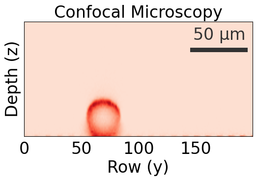
                               (a)

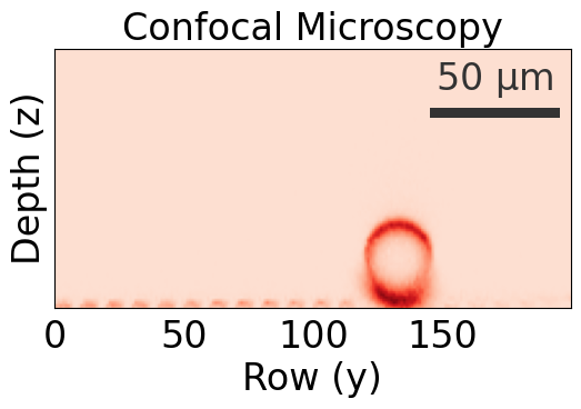
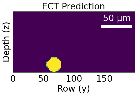
                               (b)

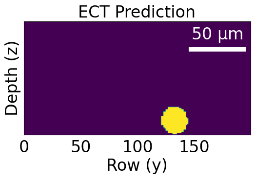
Figure 5: Image reconstruction of polymer microspheres (a) Confocal microscopy ground truth. (b) ECT model prediction.

Table I: Comparison to prior electrical capacitance tomography (ECT) systems.

[38] [39] [32] [27] [12] This Work Imaging Domain Circular Circular Circular Planar Planar Planar Reconstruction Algorithm FNN-AE FNN+CNN-AE self-attn+UNet Tikhonov Linear Back-projection TCNN+MOL Imaging Application 3D Objects 3D objects Cryogenic Fluids 3D objects Yeast cells Bacterial biofilms Electrode Size $cm$ scale $cm$ scale $cm$ scale $mm$ scale (6x6 $mm^{2}$) $mm$ scale (1.4x0.8$mm^{2}$) $\mu m$ scale (10x10$\mu m^{2}$) Array Size 8 electrodes 16 electrodes 8 electrodes 16 electrodes (4$\times$4) 34 electrodes 131,072 electrodes (512$\times$256)

III-B Bacterial Biofilm

To further develop the tomography capabilities, we aimed to produce 3-D maps of biomass within bacterial biofilms. Bacillus subtilis biofilms were grown on 500 $\mu$m-thick substrates of 1.8% agarose MSGG media for roughly 24 hours. A biofilm was cut out along with a thin supporting agarose pad and transferred onto the CMOS sensor. Before transferring the biofilm, the sensor was treated with poly-L-lysine to improve cell adhesion. The biofilm was sealed with a glass coverslip and fast-setting silicone elastomer to prevent drying, and mounted on a confocal microscope (Stellaris 5, Leica). An illustration of the completed device is shown in Fig. 3(a).

From the experimental biofilm dataset shown in Fig. 3(b), we generated 6,400 capacitance and confocal cross-sectional image pairs, which were divided into 80% training, 10% validation, and 10% testing. Fig. 6 shows the model predictions on the testing set. The results indicate that the system can accurately predict the biofilm thickness, shape, and depth from the experimental ECT measurements.

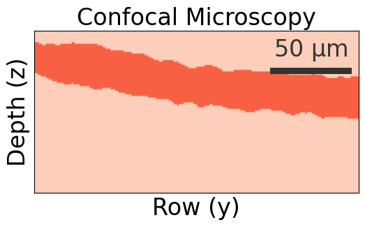
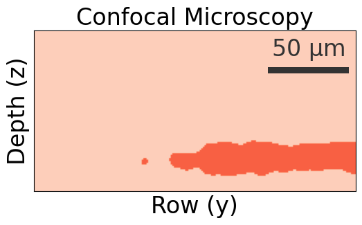
(a)

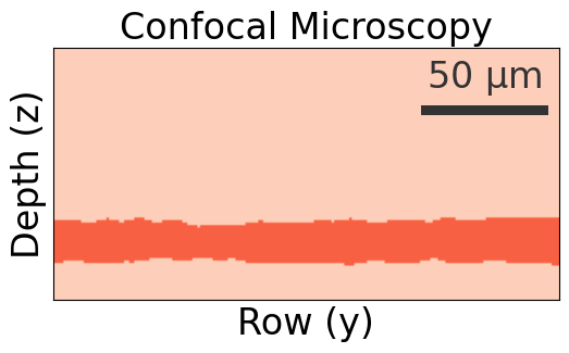
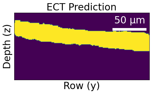
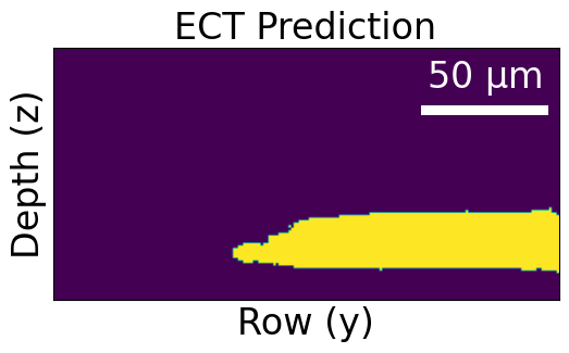
(b)

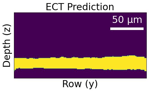
Figure 6: Reconstructed permittivity images of sections of a bacterial biofilm (a) Confocal ground truth. (b) ECT model prediction.

Predictions were performed independently on 100 $\mu$m $\times$ 200 $\mu$m meshes. However, we can reconstruct larger areas by simply stitching the predicted local meshes together. Fig. 7 shows the model predictions along a linear array of 200 electrodes (2 mm total length), demonstrating the system’s ability to resolve larger millimeter-scale features in the biofilm.

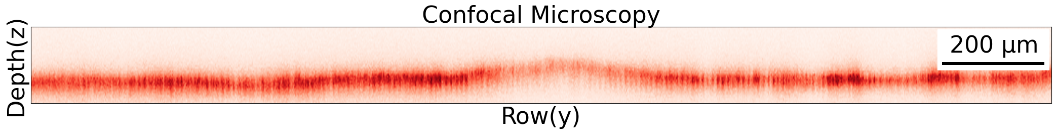
(a)

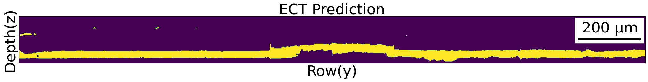
(b)

Figure 7: Reconstruction of a larger-scale cross-sectional image of a B. subtilis biofilm spanning 2 mm. (a) Confocal ground truth. (b) Model prediction, stitched together from ten 200 $\mu$m windows.

III-C Baselines

Table II: Quantitative comparison to prior work using the microsphere ($\Omega_{1}$) and biofilm ($\Omega_{2}$) datasets.

	Dataset	MSE $\downarrow$	SSIM $\uparrow$	PSNR $\uparrow$	CC $\uparrow$	IoU $\uparrow$
Tikhonov	$\Omega_{1}$	0.315	0.040	5.014	0.207	0.485
	$\Omega_{2}$	0.115	0.569	9.395	0.171	0.362
FNN-AE  [38]	$\Omega_{1}$	0.026	0.422	15.732	0.238	0.485
	$\Omega_{2}$	0.145	0.678	8.360	0.447	0.591
FNN+CNN-AE [39]	$\Omega_{1}$	0.017	0.930	17.452	0.679	0.765
	$\Omega_{2}$	0.124	0.656	9.043	0.615	0.685
self-attn+UNet [32]	$\Omega_{1}$	0.005	0.914	22.681	0.898	0.679
	$\Omega_{2}$	0.071	0.784	11.478	0.694	0.775
TCNN+MOL (Ours)	$\Omega_{1}$	0.004	0.975	23.036	0.910	0.915
	$\Omega_{2}$	0.056	0.799	12.473	0.781	0.827

We compare the reconstructions of the proposed model on the microsphere and biofilm testing datasets with one more traditional algorithm (iterative Tikhonov) and three deep learning algorithms which include the fully-connected auto-encoder (FNN-AE) presented in [38], the permittivity prediction network presented in [39] which is composed of two fully connected networks and a post-processing convolutional-based auto-encoder (FNN+CNN-AE), and the self-attention and UNet-based model (self-attn+UNet) presented in [32]. Quantitative comparisons are performed using mean squared error (MSE), and a set of perceptual metrics including structural similarity index measure (SSIM), peak signal-to-noise-ratio (PSNR), cross-correlation (CC), and intersection over union (IoU). Quantitative results are shown in Table. II and qualitative comparisons are displayed in Fig. 8. Judged by the IoU, the overall accuracy is 91.5% for the microsphere dataset, and 82.7% for the biofilm dataset.

The Tikhonov algorithm provides a good estimate for the location of the shallow bead, but fails to recognize sharp boundaries and to predict the deeper bead. This is because for planar electrodes, changes at the boundary are very subtle for relatively deep objects [6], and the Tikhonov algorithm converges to a sub-optimal reconstruction. The FNN-AE falls into a local minimum mainly because fully connected layers are not suitable for the task. While the predictions are improved by the post-processing CNN-AE, the FNN+CNN-AE also fails to predict the deeper bead. The self-attn+UNET can correctly capture the presence of the two beads, however, it underestimates the diameter of the deep bead. This is because the self-attn+UNet model is trained with the MSE loss, which is known to produce blurred/smeared predictions [21]. By incorporating a region-based loss that enhances the spatial alignment between the predictions and the ground truth images and a distribution-based loss that addresses the class-imbalance problem, our proposed model (TCNN+MOL) can predict the shape and location of both the shallow and deeper beads [28].

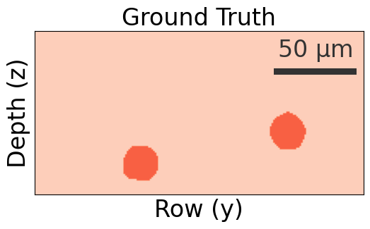
(a) Ground Truth

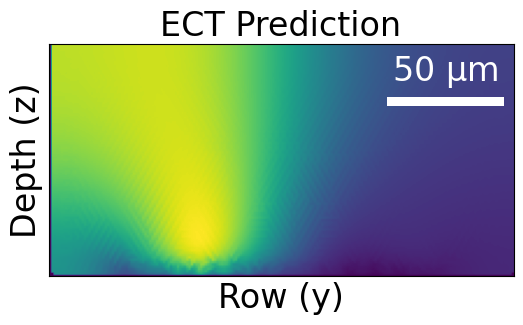
(b) Tikhonov

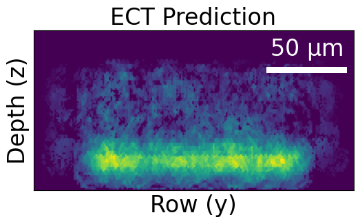
(c) FNN-AE

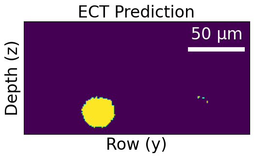
(d) FNN+CNN-AE

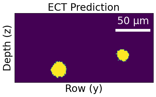
(e) self-attn+UNet

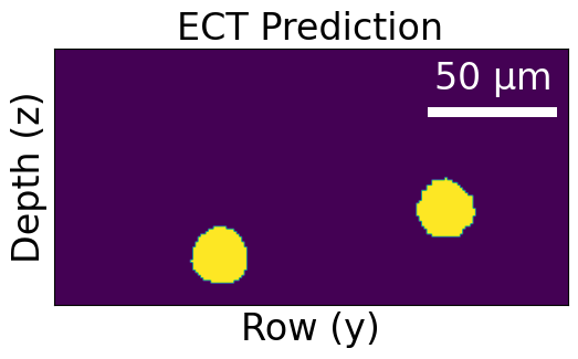
(f) TCNN+MOL (Ours)

Figure 8: Qualitative comparison to prior algorithms, using a scene of two microspheres simulated using pyEIT [20].

III-D Ablation Study

To analyze the effectiveness of the proposed approach, we conduct an ablation study on training the model with different combinations of the loss objective (Table III). In this experiment, the model was trained for 20 epochs on the biofilm dataset. We see the lowest CC when the model is trained with a per-pixel loss function ($L_{\text{Smooth L1}}$). CC is improved by adding the focal loss as it helps address the class imbalance issue. The dice loss further improves performance by maximizing overlap between the predictions and the ground truth.

Table III: Ablation on the loss function

Loss	Cross Correlation (CC)
$L_{\text{Smooth L1}}$	0.7363
$L_{\text{Smooth L1}}+L_{\text{FL}}$	0.75104
$L_{\text{Smooth L1}}+L_{\text{FL}}+L_{\text{Dice}}$	0.76320

IV Conclusion

We have presented a microscale electrical capacitance tomography (ECT) system using a CMOS biosensor that can predict the 3-D structure of objects over a large field of view. We proposed a deep learning architecture and a multi-objective training scheme for reconstructing out-of-plane images from the sensor array data. We demonstrated the effectiveness of the proposed approach by imaging polymer microspheres and bacterial biofilms. Compared to prior demonstrations (Table I), this work uses significantly smaller electrodes and achieves finer spatial resolution. Microscale ECT can be applied to a wide range of biomedical applications including low-cost non-optical label-free 3-D monitoring of cell cultures.

References

- [1] Andy Adler and Alistair Boyle. Electrical impedance tomography: Tissue properties to image measures. IEEE Transactions on Biomedical Engineering, 64(11):2494–2504, 2017.
- [2] K.J. Alme and S. Mylvaganam. Electrical capacitance tomography—sensor models, design, simulations, and experimental verification. IEEE Sensors Journal, 6(5):1256–1266, 2006.
- [3] Kirill Y Aristovich, Brett C Packham, Hwan Koo, Gustavo Sato Dos Santos, Andy McEvoy, and David S Holder. Imaging fast electrical activity in the brain with electrical impedance tomography. NeuroImage, pages 204–213, Jan 2016.
- [4] Saaid H Arshad, Jordan S Kunzika, Ethan K Murphy, Kofi Odame, and Ryan J Halter. Towards a smart phone-based cardiac monitoring device using electrical impedance tomography. In 2015 IEEE biomedical circuits and systems conference (BioCAS), pages 1–4. IEEE, 2015.
- [5] Thusara C. Chandrasekera, Yi Li, John S. Dennis, and Daniel J. Holland. Total variation image reconstruction for electrical capacitance tomography. In 2012 IEEE International Conference on Imaging Systems and Techniques Proceedings, pages 584–589, 2012.
- [6] Bo Chen and Manuchehr Soleimani. Depth analysis of planar array for 3d electrical impedance tomography. IEEE Sensors Journal, 19(22):10710–10718, 2019.
- [7] Margaret Cheney, David Isaacson, and Jonathan C. Newell. Electrical impedance tomography. SIAM Review, 41(1):85–101, 1999.
- [8] V Cherepenin, A Karpov, A Korjenevsky, V Kornienko, A Mazaletskaya, D Mazourov, and D Meister. A 3d electrical impedance tomography (eit) system for breast cancer detection. Physiological Measurement, 22(1):9, feb 2001.
- [9] Vincent Dumoulin and Francesco Visin. A guide to convolution arithmetic for deep learning. arXiv preprint arXiv:1603.07285, 2016.
- [10] Weifu Fang. A nonlinear image reconstruction algorithm for electrical capacitance tomography. Measurement Science and Technology, 15(10):2124, sep 2004.
- [11] Ross Girshick. Fast r-cnn. In 2015 IEEE International Conference on Computer Vision (ICCV), pages 1440–1448, 2015.
- [12] Xian Feng Hor, Pei Ling Leow, Mohamed Sultan Mohamed Ali, Pei Song Chee, Shahrulnizahani Mohammad Din, and Wen Pin Gooi. Electrode configuration study for three-dimensional imaging of on-chip ect. Engineering Research Express, 5(2):025003, 2023.
- [13] Kangping Hu, Christopher E Arcadia, and Jacob K Rosenstein. Super-resolution electrochemical impedance imaging with a 100 100 CMOS sensor array. In 2021 IEEE Biomedical Circuits and Systems Conference (BioCAS), pages 1–4. IEEE, 2021.
- [14] Kangping Hu, Jason Ho, and Jacob K. Rosenstein. Super-resolution electrochemical impedance imaging with a 512 × 256 CMOS sensor array. IEEE Transactions on Biomedical Circuits and Systems, 16(4):502–510, 2022.
- [15] Kangping Hu, Joseph Incandela, Xiaoyu Lian, Joseph W Larkin, and Jacob K Rosenstein. A 13.1 mm 2 512 256 multimodal CMOS array for spatiochemical imaging of bacterial biofilms. In 2022 IEEE Custom Integrated Circuits Conference (CICC), pages 1–2. IEEE, 2022.
- [16] Øyvind Isaksen. A review of reconstruction techniques for capacitance tomography. Measurement Science and Technology, 7(3):325–337, March 1996.
- [17] Yi Li, Wuqiang Yang, Cheng gang Xie, Songming Huang, Zhipeng Wu, Dimitrios Tsamakis, and Chris Lenn. Gas/oil/water flow measurement by electrical capacitance tomography. Measurement Science and Technology, 24(7):074001, jun 2013.
- [18] Tsung-Yi Lin, Priya Goyal, Ross Girshick, Kaiming He, and Piotr Dollar. Focal loss for dense object detection. In Proceedings of the IEEE International Conference on Computer Vision (ICCV), Oct 2017.
- [19] Pontus Linderholm, Laurent Marescot, Meng Heng Loke, and Philippe Renaud. Cell culture imaging using microimpedance tomography. IEEE Transactions on Biomedical Engineering, 55(1):138–146, 2007.
- [20] Benyuan Liu, Bin Yang, Canhua Xu, Junying Xia, Meng Dai, Zhenyu Ji, Fusheng You, Xiuzhen Dong, Xuetao Shi, and Feng Fu. pyeit: A python based framework for electrical impedance tomography. SoftwareX, 7:304–308, 2018.
- [21] Michaël Mathieu, Camille Couprie, and Yann LeCun. Deep multi-scale video prediction beyond mean square error. In Yoshua Bengio and Yann LeCun, editors, 4th International Conference on Learning Representations, ICLR 2016, San Juan, Puerto Rico, May 2-4, 2016, Conference Track Proceedings, 2016.
- [22] Lihui Peng, Henk Merkus, and Brian Scarlett. Using regularization methods for image reconstruction of electrical capacitance tomography. Particle & Particle Systems Characterization, 17(3):96–104, 2000.
- [23] Kshanthi Perera, Chaminda Pradeep, Saba Mylvaganam, and Rune W. Time. Imaging of oil-water flow patterns by electrical capacitance tomography. Flow Measurement and Instrumentation, 56:23–34, 2017.
- [24] Zhen Ren and Wuqiang Yang. A miniature two-plate electrical capacitance tomography sensor. IEEE Sensors Journal, 15(5):3037–3049, 2015.
- [25] Bruno MG Rosa and Guang Z Yang. Bladder volume monitoring using electrical impedance tomography with simultaneous multi-tone tissue stimulation and dft-based impedance calculation inside an fpga. IEEE Transactions on Biomedical Circuits and Systems, 14(4):775–786, 2020.
- [26] Sebastian Schlafer and Rikke L. Meyer. Confocal microscopy imaging of the biofilm matrix. Journal of Microbiological Methods, 138:50–59, 2017. What’s next in microbiology methods? Emerging methods.
- [27] Peng Suo, Jiangtao Sun, Wenbin Tian, Shijie Sun, and Lijun Xu. 3-d image reconstruction in planar array ect by combining depth estimation and sparse representation. IEEE Transactions on Instrumentation and Measurement, 70:1–9, 2021.
- [28] Saeid Asgari Taghanaki, Yefeng Zheng, S. Kevin Zhou, Bogdan Georgescu, Puneet Sharma, Daguang Xu, Dorin Comaniciu, and Ghassan Hamarneh. Combo loss: Handling input and output imbalance in multi-organ segmentation. Computerized Medical Imaging and Graphics, 75:24–33, 2019.
- [29] Warsito P. Taruno, Marlin R. Baidillah, Rommy I. Sulaiman, Muhammad F. Ihsan, Sri Elsa Fatmi, Almas H. Muhtadi, Freddy Haryanto, and Mohammed Aljohani. 4d brain activity scanner using electrical capacitance volume tomography (ecvt). In 2013 IEEE 10th International Symposium on Biomedical Imaging, pages 1006–1009, 2013.
- [30] Warsito P. Taruno, Marlin R. Baidillah, Rommy I. Sulaiman, Arbai Yusuf, Wahyu Widada, Habib Alzufri, and Muhammad Aljohani. A novel sensor design for breast cancer scanner based on electrical capacitance volume tomography (ecvt). In SENSORS, 2012 IEEE, pages 1–4, 2012.
- [31] Yu Wu, Dai Jiang, Xiao Liu, Richard Bayford, and Andreas Demosthenous. A human–machine interface using electrical impedance tomography for hand prosthesis control. IEEE transactions on biomedical circuits and systems, 12(6):1322–1333, 2018.
- [32] Gao Xinxin, Tian Zenan, Qiu Limin, and Zhang Xiaobin. A hybrid deep learning model for ect image reconstruction of cryogenic fluids. Flow Measurement and Instrumentation, 87:102228, 2022.
- [33] W Q Yang and Lihui Peng. Image reconstruction algorithms for electrical capacitance tomography. Measurement Science and Technology, 14(1):R1, dec 2002.
- [34] W Q Yang, D M Spink, T A York, and H McCann. An image-reconstruction algorithm based on landweber’s iteration method for electrical-capacitance tomography. Measurement Science and Technology, 10(11):1065, nov 1999.
- [35] Michael Yeung, Evis Sala, Carola-Bibiane Schönlieb, and Leonardo Rundo. Unified focal loss: Generalising dice and cross entropy-based losses to handle class imbalanced medical image segmentation. Computerized Medical Imaging and Graphics, 95:102026, 2022.
- [36] Rongjian Zhao, Buyue Qian, Xianli Zhang, Yang Li, Rong Wei, Yang Liu, and Yinggang Pan. Rethinking dice loss for medical image segmentation. In 2020 IEEE International Conference on Data Mining (ICDM), pages 851–860, 2020.
- [37] Jin Zheng, Haocheng Ma, and Lihui Peng. A cnn-based image reconstruction for electrical capacitance tomography. In 2019 IEEE International Conference on Imaging Systems and Techniques (IST), pages 1–6, 2019.
- [38] Jin Zheng and Lihui Peng. An autoencoder-based image reconstruction for electrical capacitance tomography. IEEE Sensors Journal, 18(13):5464–5474, 2018.
- [39] Hai Zhu, Jiangtao Sun, Lijun Xu, Wenbin Tian, and Shijie Sun. Permittivity reconstruction in electrical capacitance tomography based on visual representation of deep neural network. IEEE Sensors Journal, 20(9):4803–4815, 2020.