A posteriori error control for a Discontinuous Galerkin approximation of a Keller-Segel model

Abstract

We provide a posteriori error estimates for a discontinuous Galerkin scheme for the parabolic-elliptic Keller-Segel system in 2 or 3 space dimensions. The estimates are conditional, in the sense that an a posteriori computable quantity needs to be small enough - which can be ensured by mesh refinement - and optimal in the sense that the error estimator decays with the same order as the error under mesh refinement. A specific feature of our error estimator is that it can be used to prove existence of a weak solution up to a certain time based on numerical results.

Keywords: Keller-Segel; chemotaxis; nonlinear diffusion; discontinuous Galerkin scheme; a posteriori error analysis

AMS subject classification (2020): Primary 65M50, Secondary 65M08, 35K40

1 Introduction

The Keller-Segel system is a well-known mathematical model in the field of chemotaxis. Introduced by E. Keller and L. Segel [23], it describes the collective motion of cells in response to concentration gradients. It consists of two coupled partial differential equations:

$$\begin{matrix}\begin{aligned} \partial_{t}\rho+\nabla\cdot(\chi\rho\nabla c-\nabla\rho)&=0\\ \epsilon\partial_{t}c+c-\Delta c-\alpha\rho&=0\end{aligned}\end{matrix}$$ (1)

and suitable initial and boundary conditions. Here $\rho=\rho(t,x)$ and $c=c(t,x)$ denote the density of the cell population and the concentration of chemically attracting substances, respectively, for any time $t>0$ at location $x\in\Omega$. We will consider the problem on a bounded open set $\Omega$ in $\mathbb{R}^{d}$ with a piecewise smooth boundary $\partial\Omega$. The parameters $\chi$, $\alpha$, and $\epsilon$ are constant and satisfy $\chi,\alpha>0$ and $\epsilon\geq 0$. The modelling background of this system has been extensively discussed in the literature [17, 30], and there are large number of extensions, e.g. models accounting for multiple stimuli and multiple species [41, 20, 22].

In this work, we focus on the parabolic-elliptic form of the Keller-Segel system described by the partial differential equations (1) when $\epsilon=0$ (and setting the other parameters to $1$ for simplicity):

$$\partial_{t}\rho+\nabla\cdot(\rho\nabla c-\nabla\rho) =0\quad\text{in}\ (0,T)\times\Omega$$ (2)

$$c-\Delta c =\rho\quad\text{in}\ (0,T)\times\Omega$$ (3)

$$\nabla\rho\cdot\mathrm{n} =0\quad\text{on}\ (0,T)\times\partial\Omega$$ (4)

$$\nabla c\cdot\mathrm{n} =0\quad\text{on}\ (0,T)\times\partial\Omega$$ (5)

$$\rho(0,\cdot) =\rho_{0}\quad\text{in}\ \Omega$$ (6)

where $\mathrm{n}$ denotes the outward unit normal vector.

A striking feature of the Keller-Segel system which motivates detailed investigations is the finite time blow-up of solutions [31]. Such singularities are expected in settings of dimension $d\geq 2$ when the initial cell population surpasses a certain threshold. For $d=2$, this threshold is on the total mass [13, 6] and for $d\geq 3$, it depends on the maximal local concentration. For an overview on the Keller-Segel system, we refer to the review papers [18, 19].

For special initial data explicit formulas for blow up solutions exist but, in general, approximating solutions of this system with blow-up accurately is challenging. Several numerical methods have been developed over the years to tackle this issue. These methods include the fractional step method [39], finite volume schemes [12, 9], and conservative upwind finite-element methods [35, 36]. Additionally, [11, 26] employed discontinuous Galerkin methods, and [7] utilized a moving mesh method.

More generally, solutions to chemotaxis systems frequently display strong growth of cell density close to some point or curve. Indeed, the system may not only exhibit blow-up but it may also develop other ‘spiky’ structures. Resolving such highly localized structures on uniform meshes is, arguably, inefficient and there has been an intense interest in the development of (mesh) adaptive numerical schemes [10, 37] with the goal of increasing accuracy and efficiency. Several heuristic strategies for mesh adaptation can be found in the literature, e.g., [37] presents an adaptive moving mesh finite element method, using a coordinate transformation to concentrate grid nodes in regions of large solution variations, and [10], which proposes a semi-discrete adaptive moving mesh finite-volume upwind method, enhancing resolution in blow-up regions by increasing the density of mesh nodes. To the best of our knowledge, mesh adaptation based on a posteriori error estimates has not been investigated. The goal of this work is to provide a basis for such investigations. At the same time, our results provide rigorous error control of simulations.

Mesh adaptation based on a posteriori error estimates has been extremely successful for simpler types of PDEs, even leading to provably optimal meshes in certain cases. For instance, convergence of an adaptive space-time finite element method that relies on an a posteriori error estimator for solving linear parabolic partial differential equations was proven in [24]. A posteriori error estimates come in several varieties: If there is a goal functional of specific interest dual weighted residuals may be used, see e.g. [2], which usually leads to very efficient meshes. We follow a different approach that aims at controlling the error in a suitable norm and is nicely explained in [27]. The main idea is to insert a (sufficiently regular) reconstruction of the numerical solution into the PDE so that a suitable stability theory can be used to bound the difference between the exact solution to the PDE and this reconstruction. For nonlinear equations it may happen that the stability theory allows only conditional a posteriori error estimates, e.g. the Allen-Cahn equation [1], and this is indeed the case here.

Different stability frameworks, e.g. ones based on (relative) entropy or negative order norms, could be considered for the Keller-Segel system. We present an a posteriori error estimate using a rather standard $L^{2}$-based stability framework since this is the framework that, for us, leads to the strongest results. It might seem that using an $L^{2}$-based stability framework requires unrealistic and unverifiable assumptions on the regularity of exact solutions but it turns out that, for sufficiently regular initial data, weak solutions retain this regularity until blow-up time [5] and we provide an a posteriori verifiable condition that guarantees that the exact solution is sufficiently regular.

The numerical scheme studied in this manuscript is a straightforward discontinuous Galerkin (dG) scheme. Much more sophisticated schemes have been developed in the literature, e.g. [16, 34], offering features such as entropy dissipation and positivity preservation. It is beyond the scope of the current work to extend our error estimator to those schemes but it should be noted that several results from this paper, in particular Theorem 3.2, can be directly used for the analysis of those schemes, e.g. the companion paper [14] provides suitable reconstructions and an $H^{-1}$-norm estimate for the residual for a positivity preserving finite volume scheme.

Our analysis is performed in the semi-(spatially)-discrete setting since, arguably, this already covers the key challenges. Our results can be combined with ideas from the study of a posteriori error estimates for temporal discretisation of PDEs with blow-up [8, 25]. It is worth noting that the error estimator presented in our work is of optimal order, i.e. the error estimator has the same order of convergence as the norm of the error that it controls.

We investigate a semi-discrete discontinuous Galerkin (dG) scheme discretising Laplace operators by the symmetric interior penalty (SIP) bilinear form and the chemotaxis term by the weighted SIP (wSIP) bilinear form treating density as a diffusion coefficient. Our analysis applies to arbitrary polynomial degrees $k\geq 1$.

The outline of the paper is as follows: In Section 2, we provide some background on weak solutions for the Keller-Segel system, with a focus on blow-up phenomena. In Section 3, we establish a stability estimate for the strong solution of the system, serving as the foundation for constructing the a posteriori error estimator. It is worth noting that this stability estimate can, in certain situations, a posteriori verify the existence of a sufficiently regular weak solution. In Section 4, we introduce our semi-spatial-discrete discontinuous Galerkin scheme. In Section 5, we define the reconstruction of the numerical solution, utilizing the so-called elliptic reconstruction, and also define the residual. In Section 6, we derive a computable upper bound for the $H^{-1}$-norm of the residual. Section 7, which delineates our main result, presents the full a posteriori error estimator. Finally, in Section 8, we conduct numerical experiments.

2 Background on weak solutions and blow-up

We study the parabolic-elliptic Keller-Segel system with Neumann boundary conditions (2)–(6). The existence of a local-in-time weak solution for this problem is well established [5, Section 3]. Let us recall the definition of a weak solution as given in [5]:

Definition 2.1.

[5] A function $\rho\in L^{\infty}\left(0,T;L^{2}(\Omega)\right)\cap L^{2}\left(0,T;H^{1}(\Omega)\right)$ is called a weak solution of the problem (2)-(6) on $\left(0,T\right)\times\Omega$, if it satisfies

$$\int_{\Omega}\rho(t,x)\varphi(t,x)dx-\int_{0}^{t}\int_{\Omega}\rho\partial_{t}\varphi-(\nabla\rho-\rho\nabla c)\cdot\nabla\varphi dxds\\ =\int_{\Omega}\rho_{0}(x)\varphi(0,x)dx$$

for every $\varphi\in H^{1}((0,T)\times\Omega)$ and for a.e. $t\in(0,T)$ and, if, in addition, for a.e. $t\in(0,T)$

$$c(t,\cdot)\in H^{1}(\Omega)\text{ with }c(t,x)=(G*\rho(t,\cdot))\left(x\right)\quad\text{for a.e.}\ x\in\Omega$$

holds, where $G$ is an appropriate Green’s function for $\Omega$.

Theorem 2.2 (Existence of weak solutions).

[5, Theorem 2] Assume that $\Omega$ is a bounded domain in $\mathbb{R}^{d}$ with piecewise smooth boundary.

1. If $d\in\{2,3\}$, and $0\leq\rho_{0}\in L^{2}(\Omega)$, then there exists $T=$ $T\left(\left\|\rho_{0}\right\|_{L^{2}(\Omega)}\right)$ such that the problem (2)-(6) has a unique weak solution $\rho\in$ $L^{\infty}\left(0,T;L^{2}(\Omega)\right)\cap L^{2}\left(0,T;H^{1}(\Omega)\right)$. Moreover, $\partial_{t}\rho\in L^{2}\left(0,T;H^{-1}(\Omega)\right)$, $\rho(t,x)\geq 0$ for a.e. $x\in\Omega$ and $t\geq 0$, and $\int_{\Omega}\rho(t,x)dx=\int_{\Omega}\rho_{0}(x)dx$.

2. If $d\geq 2$ and $0\leq\rho_{0}\in L^{p}(\Omega),p>d/2$, then there exists $T=$ $T\left(p,\left\|\rho_{0}\right\|_{L^{p}(\Omega)}\right)>0$ and a weak solution $\rho$ such that $\rho\in L^{\infty}\left(0,T;L^{p}(\Omega)\right)$ and $\rho^{p/2}\in L^{2}\left(0,T;H^{1}(\Omega)\right)$. These solutions are unique when $p>d$, and regular when $p>d/2$ in the sense that $\rho\in L_{\mathrm{loc}}^{\infty}\left(0,T;L^{\infty}(\Omega)\right)$.

Remark 2.3.

With (i) of Theorem 2.2, a routine calculation, e.g. [4] and references therein, shows that such a weak solution satisfies $\rho\in C\left([0,T];L^{2}(\Omega)\right)$, and the energy balance

$$\frac{1}{2}\int_{\Omega}\rho^{2}(t,x)dx+\int_{0}^{t}\int_{\Omega}(\nabla\rho-\rho\nabla c)\cdot\nabla\rho=\frac{1}{2}\int_{\Omega}\rho_{0}^{2}(x)dx.$$

Moreover, by the representation $c=G*\rho$, we know that $c\in C([0,T];H^{1}(\Omega))$. For notational convenience, we abuse the differential form throughout this paper:

$$\frac{1}{2}\frac{d}{dt}\left\|\rho(t,\cdot)\right\|_{L^{2}(\Omega)}^{2}+\left\|\nabla\rho(t,\cdot)\right\|_{L^{2}(\Omega)}^{2}=\int_{\Omega}\rho(t,\cdot)\nabla c(t,\cdot)\cdot\nabla\rho(t,\cdot).$$ (7)

This is obtained through a formal process that involves computing the $L^{2}$ inner product of the equation with $\rho$, followed by an integration by parts.

We make several observations regarding the characteristics of blow-up of solutions which will play a crucial role in our a posteriori analysis in Section 3.

Remark 2.4.

We remark that (ii) of Theorem (2.2) means that if a solution blows up at some time $T>0$ (i.e. $\lim_{t\rightarrow T}\left\|\rho(t,\cdot)\right\|_{L^{\infty}(\Omega)}=\infty$), then the norms $\left\|\rho(t,\cdot)\right\|_{L^{p}(\Omega)}$ blow up for all $p\in(d/2,\infty]$ at the same moment [5, p.333].

Remark 2.5.

Let $T_{max}\in(0,+\infty]$ be the maximal existence time of the solution, that is, the supremum of all $T>0$ such that the solution exists on $[0,T]$. If $T_{max}<\infty$, we have

$$\lim_{t\rightarrow T_{max}}\left\|\rho(t,\cdot)\right\|_{L^{\infty}(\Omega)}=\infty.$$ (8)

The existing literature, e.g. [38, Theorem 3.2], provides a proof of the blow-up criterion for classical solutions to the Keller-Segel system. However, despite the possibility of establishing this property for weak solutions through the energy method we could not find a detailed proof for weak solutions in the literature. Since this property is crucial for the proof of Corollary 3.3, we present a rigorous proof for the blow-up criterion with respect to weak solutions in this context.

Proof of Remark 2.5.

Assume that equation (8) does not hold. We can then extract a sequence $\left\{t_{k}\right\}_{k=1}^{\infty}$, such that $\left\|\rho(t_{k},\cdot)\right\|_{L^{\infty}(\Omega)}<C$ for all $k$, and where $t_{k}$ approaches $T_{max}$ from below as $k$ tends to infinity. Since $\Omega$ is bounded, we have $\left\|\rho(t_{k},\cdot)\right\|_{L^{2}(\Omega)}\leq C$ for all $k$. Now if we use each $t_{k}$ as an initial time point, the local existence theorem enables us to define an interval $[t_{k},t_{k}+\delta_{k})$ with $\delta_{k}=\delta_{k}\left(\left\|\rho(t_{k},\cdot)\right\|_{L^{2}(\Omega)}\right)>0$ on which a solution exists.. We note that all initial data $\left\|\rho(t_{k},\cdot)\right\|_{L^{2}(\Omega)}$ possess a uniform upper bound. As shown in [3, the proof of Theorem 1], this means the sequence $\left\{\delta_{k}\right\}$ does not shrink to zero, allowing us to define $\delta:=\inf_{k}\delta_{k}>0$. Consequently, we can choose $k_{0}\in\mathbb{N}$ such that $T_{max}-\frac{1}{2}\delta<t_{k_{0}}$. By employing the continuation argument, we find that the weak solution exists until $t_{k_{0}}+\delta>T_{max}$, a contradiction to the definition of $T_{max}$. Thus, (8) holds true. ∎

The stability framework that will be presented in the next section requires that $c$ can be controlled by sufficiently weak norms of $\rho$, i.e. elliptic regularity for (3)–(5). Since (3) has constant coefficients this depends on properties of $\Omega$. A sufficient condition is that $\Omega$ is convex.

Assumption 2.6.

Throughout this paper, we assume $d\in\{2,3\}$ and that $\Omega$ is such that (3), (5) enjoys elliptic regularity, i.e. there exists a positive constant $C_{ell}>0$, depending only on $\Omega$, such that $\|c(t,\cdot)\|_{H^{2}}\leq C_{ell}\|\rho\left(t,\cdot\right)\|_{L^{2}}$ for all $t$.

3 A stability framework

Let $\left(\rho,c\right)$ be a weak solution to the problem (2)-(6) and let $\left(\bar{\rho},\bar{c}\right)$ with $\bar{\rho}\in C\left([0,T];H^{1}(\Omega)\right)$, $\partial_{t}\bar{\rho}\in C\left((0,T];H^{-1}(\Omega)\right)$, $\bar{c}\in C\left([0,T];H^{2}(\Omega)\right)$ be a strong solution to the following perturbed problem:

$$\partial_{t}\bar{\rho}+\nabla\cdot(\bar{\rho}\nabla\bar{c}-\nabla\bar{\rho}) =R_{\rho}\quad\text{ in }(0,T)\times\Omega$$ (9)

$$\bar{c}-\Delta\bar{c} =\bar{\rho}\quad\text{ in }(0,T)\times\Omega$$ (10)

$$\nabla\rho\cdot\mathrm{n} =0\quad\text{ on }(0,T)\times\partial\Omega$$ (11)

$$\nabla c\cdot\mathrm{n} =0\quad\text{ on }(0,T)\times\partial\Omega$$ (12)

with some given function $R_{\rho}\in L^{2}(0,T;H^{-1}(\Omega))$. We are going to provide an estimate for the difference $(\rho-\bar{\rho},c-\bar{c})$ in terms of the (possible) difference of initial data and of $R_{\rho}$. The situation we have in mind is that $\bar{\rho},\bar{c}$ is a reconstruction of a numerical solution as in Section 5. However, it is important to note that our stability framework does not depend on how $\bar{\rho},\bar{c}$ was obtained.

Taking into account Remark 2.3, we will subsequently provide a formal argument for the derivation of the stability estimate, but it can be made rigorous by interpreting it in the context of appropriate integral formulations. For the sake of brevity, we choose not to explicitly include $\Omega$ in the norm symbols. Furthermore, the time dependency of functions will also not be explicitly denoted. Subtracting (9) from (2) and testing with $\rho-\bar{\rho}$ we obtain

$$\frac{d}{dt}\left[\int_{\Omega}\frac{1}{2}(\rho-\bar{\rho})^{2}dx\right]+\int_{\Omega}|\nabla(\rho-\bar{\rho})|^{2}dx\\ =\int_{\Omega}\nabla(\rho-\bar{\rho})\bar{\rho}\nabla(c-\bar{c})+\nabla(\rho-\bar{\rho})(\rho-\bar{\rho})\nabla\bar{c}-R_{\rho}(\rho-\bar{\rho})+\nabla(\rho-\bar{\rho})(\rho-\bar{\rho})\nabla(c-\bar{c})dx,$$

where we used the homogeneous boundary conditions. Using Cauchy-Schwarz’s inequality we obtain

$$\frac{d}{dt}\left[\frac{1}{2}\|\rho-\bar{\rho}\|_{L^{2}}^{2}\right]+|\rho-\bar{\rho}|_{H^{1}}^{2}\\ \leq|\rho-\bar{\rho}|_{H^{1}}\|\bar{\rho}\|_{L^{3}}|c-\bar{c}|_{W^{1,6}}+|\rho-\bar{\rho}|_{H^{1}}\|\rho-\bar{\rho}\|_{L^{2}}\|\nabla\bar{c}\|_{L^{\infty}}\\ \quad+\|R_{\rho}\|_{H^{-1}}\|\rho-\bar{\rho}\|_{H^{1}}+|\rho-\bar{\rho}|_{H^{1}}\|\rho-\bar{\rho}\|_{L^{3}}|c-\bar{c}|_{W^{1,6}}.$$

Since the number of space dimensions satisfies $d\leq 3$, we have $\left|c-\bar{c}\right|_{W^{1,6}}\leq C_{S}\left\|\nabla c-\nabla\bar{c}\right\|_{H^{1}}$, and $\left\|\rho-\bar{\rho}\right\|_{L^{3}}\leq C_{S}^{\prime}\left\|\rho-\bar{\rho}\right\|_{H^{1}}$ where $C_{S},C_{S}^{\prime}$ are the constants of the embedding $H^{1}\rightarrow L^{6}$ and $H^{1}\rightarrow L^{3}$, respectively. Moreover, by elliptic regularity, we have $\left\|c-\bar{c}\right\|_{H^{2}}\leq C_{ell}\left\|\rho-\bar{\rho}\right\|_{L^{2}}$. This implies

$$\frac{d}{dt}\left[\frac{1}{2}\|\rho-\bar{\rho}\|_{L^{2}}^{2}\right]+|\rho-\bar{\rho}|_{H^{1}}^{2}\\ \leq C_{S}C_{ell}|\rho-\bar{\rho}|_{H^{1}}\|\bar{\rho}\|_{L^{3}}\left\|\rho-\bar{\rho}\right\|_{L^{2}}+|\rho-\bar{\rho}|_{H^{1}}\|\rho-\bar{\rho}\|_{L^{2}}\|\nabla\bar{c}\|_{L^{\infty}}\\ +\|R_{\rho}\|_{H^{-1}}\|\rho-\bar{\rho}\|_{H^{1}}+C_{S}^{\prime}C_{S}C_{ell}|\rho-\bar{\rho}|_{H^{1}}\|\rho-\bar{\rho}\|_{H^{1}}\left\|\rho-\bar{\rho}\right\|_{L^{2}}.$$

Using Young’s inequality and gathering terms on the right hand side, we obtain

$$\frac{d}{dt}\left[\left\|\rho-\bar{\rho}\right\|_{L^{2}}^{2}\right]+\left|\rho-\bar{\rho}\right|_{H^{1}}^{2}\leq\left(3C_{S}^{2}C_{ell}^{2}\left\|\bar{\rho}\right\|_{L^{3}}^{2}+3\left\|\nabla\bar{c}\right\|_{L^{\infty}}^{2}+\frac{1}{3}\right)\left\|\rho-\bar{\rho}\right\|_{L^{2}}^{2}\\ +3\left\|R_{\rho}\right\|_{H^{-1}}^{2}+2C_{S}^{\prime}C_{S}C_{ell}|\rho-\bar{\rho}|_{H^{1}}\|\rho-\bar{\rho}\|_{H^{1}}\|\rho-\bar{\rho}\|_{L^{2}}.$$ (13)

Let us set

$$\begin{split}y_{1}(t)&:=\|\rho(t,\cdot)-\bar{\rho}(t,\cdot)\|_{L^{2}}^{2},\\ y_{2}(t)&:=|\rho(t,\cdot)-\bar{\rho}(t,\cdot)|_{H^{1}}^{2},\\ y_{3}(t)&:=2C_{S}^{\prime}C_{S}C_{ell}|\rho(t,\cdot)-\bar{\rho}(t,\cdot)|_{H^{1}}\|\rho(t,\cdot)-\bar{\rho}(t,\cdot)\|_{H^{1}}\|\rho(t,\cdot)-\bar{\rho}(t,\cdot)\|_{L^{2}},\\ a(t)&:=3C_{S}^{2}C_{ell}^{2}\|\bar{\rho}(t,\cdot)\|_{L^{3}}^{2}+3\|\nabla\bar{c}(t,\cdot)\|_{L^{\infty}}^{2}+\frac{1}{3}.\end{split}$$ (14)

Then, we can integrate (13) in time from $0$ to $T^{\prime}$ to obtain

$$y_{1}(T^{\prime})+\int_{0}^{T^{\prime}}y_{2}(t)dt\leq y_{1}(0)+\int_{0}^{T^{\prime}}\|R_{\rho}\|_{H^{-1}}^{2}dt+\int_{0}^{T^{\prime}}a(t)y_{1}(t)dt+\int_{0}^{T^{\prime}}y_{3}(t)dt$$ (15)

Since $\left\|\rho-\bar{\rho}\right\|_{H^{1}}^{2}=\left\|\rho-\bar{\rho}\right\|_{L^{2}}^{2}+\left|\rho-\bar{\rho}\right|_{H^{1}}^{2}$, we have

$$y_{3}(t)\leq 2C_{S}^{\prime}C_{S}C_{ell}\|\rho-\bar{\rho}\|_{H^{1}}^{2}\|\rho-\bar{\rho}\|_{L^{2}}\\ \leq 2C_{S}^{\prime}C_{S}C_{ell}\sqrt{y_{1}(t)}(y_{1}(t)+y_{2}(t)).$$ (16)

In the final inequality, we have used Young’s inequality. This leads us to:

$$\int_{0}^{T^{\prime}}y_{3}(t)dt\leq 2C_{S}^{\prime}C_{S}C_{ell}\sup_{t}\sqrt{y_{1}(t)}\int_{0}^{T^{\prime}}y_{1}(t)+y_{2}(t)dt.$$ (17)

Equations (15) and (17) show that our analysis fits into the framework of Proposition 3.1 with $y_{1},y_{2},y_{3},$ and $a$ as above; $B:=2C_{S}^{\prime}C_{S}C_{ell}$, $\beta=\frac{1}{2}$,

$$A:=y_{1}(0)+\int_{0}^{T}\|R_{\rho}\|_{H^{-1}}^{2}dt,\quad\text{and}\quad E:=\exp\left(\int_{0}^{T}a(t)dt\right).$$ (18)

Proposition 3.1.

[1, Prop 6.2, Generalized Gronwall lemma] Suppose that nonnegative functions $y_{1}\in C([0,T]),y_{2},y_{3}\in L^{1}([0,T]),a\in L^{\infty}([0,T])$, and a real number $A\geq 0$ satisfy

$$y_{1}\left(T^{\prime}\right)+\int_{0}^{T^{\prime}}y_{2}(t)\mathrm{d}t\leq A+\int_{0}^{T^{\prime}}a(t)y_{1}(t)\mathrm{d}t+\int_{0}^{T^{\prime}}y_{3}(t)\mathrm{d}t$$

for all $T^{\prime}\in[0,T]$ and that, in addition, for $B\geq 0,\beta>0$, and every $T^{\prime}\in[0,T]$

$$\int_{0}^{T^{\prime}}y_{3}(t)\mathrm{d}t\leq B\left(\sup_{t\in\left[0,T^{\prime}\right]}y_{1}^{\beta}(t)\right)\int_{0}^{T^{\prime}}\left(y_{1}(t)+y_{2}(t)\right)\mathrm{d}t.$$

Let $E:=\exp\left(\int_{0}^{T}a(t)\mathrm{d}t\right)$. Then, provided $8AE\leq(8B(1+T)E)^{-1/\beta}$ is satisfied the following inequality holds:

$$\sup_{t\in[0,T]}y_{1}(t)+\int_{0}^{T}y_{2}(t)\mathrm{d}t\leq 8A\exp\left(\int_{0}^{T}a(s)\mathrm{d}s\right).$$

Thus, we have the following conditional stability result:

Theorem 3.2.

For fixed $T>0$, let $\left(\rho,c\right)$ be a weak solution to (2)-(6) and $\left(\bar{\rho},\bar{c}\right)$ a strong solution to (9)–(12). Let $y_{1},y_{2},y_{3},$ and $a$ be defined as in (14) and $B=2C_{S}^{\prime}C_{S}C_{ell}$, $\beta=\frac{1}{2}$, and $A,\,E$ as in (18). Then, provided

$$8AE(8B(1+T)E)^{2}\leq 1,$$ (19)

is satisfied, the difference $\rho-\bar{\rho}$ is controlled as follows:

$$\sup_{t\in[0,T]}\|\rho(t,\cdot)-\bar{\rho}(t,\cdot)\|_{L^{2}(\Omega)}^{2}+\int_{0}^{T}|\rho(t,\cdot)-\bar{\rho}(t,\cdot)|_{H^{1}(\Omega)}^{2}dt\\ \leq 8\left(\|\rho(0,\cdot)-\bar{\rho}(0,\cdot)\|_{L^{2}(\Omega)}^{2}+\int_{0}^{T}\|R_{\rho}\|_{H^{-1}(\Omega)}^{2}dt\right)\\ \times\exp\left(\int_{0}^{T}3C_{S}^{2}C_{ell}^{2}\|\bar{\rho}(t,\cdot)\|_{L^{3}(\Omega)}^{2}+3\|\nabla\bar{c}(t,\cdot)\|_{L^{\infty}(\Omega)}^{2}+\frac{1}{3}dt\right).$$ (20)

Note that the stability framework presented here is independent of the origin of the approximate solution $(\bar{\rho},\bar{c})$. Moreover, the assumption that a weak solution $(\rho,c)$ exists until time $T$ is a posteriori verifiable. Indeed, if (19) holds, the error estimate itself rules out blow-up before time $T$ and thus proves a posteriori that a sufficiently regular weak solution exists. More precisely:

Corollary 3.3.

Given any initial data $\rho_{0}\in L^{2}(\Omega)$, let $T_{max}>0$ be the maximal existence time of the weak solution $\rho$ to (2)-(6). Let there exist an approximate strong solution $\bar{\rho}$, i.e. a solution of (9)–(12) such that at some time $T>0$ the condition (19) is satisfied, $\|\bar{\rho}\|_{L^{\infty}(0,T;L^{2}(\Omega))}$ is finite and the right hand side of (20) is finite, then $T_{max}>T$, i.e., the weak solution exists at least until time $T$.

Proof.

If (19) holds for some time $T>0$ then it also holds for all earlier times, since the left hand side of (19) is increasing in time. Suppose $T_{max}<T$. Then, (20) evaluated at time $T$ provides a uniform upper bound for $\|\rho(t,\cdot)\|_{L^{2}(\Omega)}$ for almost all $t\in[0,T_{max}]$, by bounding its distance from $\bar{\rho}(t,\cdot)$.

In contrast, the blow-up property, explained in Remark 2.4 and Remark 2.5, implies that the $L^{2}$-norm of $\rho$ must blow up for $t\rightarrow T_{max}$, since $d\leq 3$. This is a contradiction. ∎

4 A semi-discrete Discontinuous Galerkin Scheme

In order to keep our paper self-contained, we begin this section by briefly recalling some basic notations. Details can be found in, e.g. [33]. We employ a discontinuous Galerkin (dG) finite element method for spatial discretisation.

Definition 4.1 (Finite element space).

Let $\Omega$ be decomposed into a set $\mathcal{T}$ of disjoint polyhedra $\{T\}$. Let $h_{T}$ denote the diameter of $T$. We use the notation $\mathcal{T}_{h}$ for a mesh $\mathcal{T}$ with mesh size $h$. We define $\mathcal{F}_{h}^{i}$ as the set of common interfaces of cells in the mesh $\mathcal{T}_{h}$, and $\mathcal{F}_{h}^{b}$ as the set of boundary faces on the boundary $\partial\Omega$. We set

$$\mathcal{F}_{h}:=\mathcal{F}_{h}^{i}\cup\mathcal{F}_{h}^{b},$$

as the set of all faces in the mesh. For all $F\in\mathcal{F}_{h}$, in dimension $d\geq 2$, we set $h_{F}$ to be equal to the diameter of the face $F$, while, in dimension 1 , we set $h_{F}:=\min\left\{h_{T_{1}},h_{T_{2}}\right\}$ if $F\in\mathcal{F}_{h}^{i}$ with $F=\partial T_{1}\cap\partial T_{2}$ and $h_{F}:=h_{T}$ if $F\in\mathcal{F}_{h}^{b}$ with $F=\partial T\cap\partial\Omega$. Furthermore, for any $T\in\mathcal{T}_{h}$, we set

$$\mathcal{F}_{T}:=\left\{F\in\mathcal{F}_{h}\mid F\subset\partial T\right\},$$ (21)

which collects the mesh faces comprising the boundary of $T$.

We say that a mesh sequence $\mathcal{T}_{h}$ is admissible if it is shape- and contact-regular and if it has optimal polynomial approximation properties. Definitions of these notions can be found in [33, Section 1.4]. Throughout this paper, we always assume that the mesh sequence $\mathcal{T}_{h}$ is admissible.

Let $\mathbb{P}_{d}^{k}$ denote the space of polynomials of degree less than or equal to $k$. We define the discontinuous finite element space as

$$V_{h}:=\mathbb{P}_{d}^{k}(\mathcal{T}_{h}):=\{v:\Omega\to\mathbb{R}\,:\,v|_{T}\in\mathbb{P}_{d}^{k}{(T)}\ \forall\,T\in\mathcal{T}_{h}\}$$ (22)

with polynomial degree $k\geq 1$.

Definition 4.2 (Broken Sobolev spaces and broken gradients).

We introduce the broken Sobolev space

$$W^{m,p}\left(\mathcal{T}_{h}\right) :=\left\{v\in L^{p}(\Omega)\,:\,v|_{T}\in W^{m,p}(T),\text{ for each }T\in\mathcal{T}_{h}\right\}.$$ (23)

For $p=2$, we set $H^{m}(\mathcal{T}_{h}):=W^{m,2}\left(\mathcal{T}_{h}\right)$. We also make use of functions defined in these broken spaces restricted to the skeleton of the mesh.
The broken gradient $\nabla_{h}:W^{1,p}\left(\mathcal{T}_{h}\right)\rightarrow$ $\left[L^{p}(\Omega)\right]^{d}$ is defined, by

$$\forall v\in W^{1,p}\left(\mathcal{T}_{h}\right)\quad\forall T\in\mathcal{T}_{h},\left.\quad\left(\nabla_{h}v\right)\right|_{T}:=\nabla\left(\left.v\right|_{T}\right).$$

Definition 4.3 (Weighted averages and jumps).

For any interface $F\in\mathcal{F}_{h}^{i}$ let $\omega^{+},\omega^{-}\in W^{1,\infty}(F)$ be weight functions that are uniformly bounded from below by a positive real number. Let $F=\partial T_{1}\cap\partial T_{2}$ then we define, for a.e. $x\in F$, the weighted average and jump:

$$\mathopen{\scalebox{1.0}{$\{\!\mkern-1.0mu\{$}}v\mathclose{\scalebox{1.0}{$\}\!\mkern-1.0mu\}$}}_{\omega,F}(x):=\left.\omega^{+}_{F}v\right|_{T_{1}}(x)+\left.\omega^{-}_{F}v\right|_{T_{2}}(x),$$ (24)

and

$$\llbracket v\rrbracket_{F}(x):=\left.v\right|_{T_{1}}(x)-\left.v\right|_{T_{2}}(x).$$ (25)

The weighted averages and jumps are defined for boundary faces by setting, for a. e. $x\in F$ with $F\in\mathcal{F}_{h}^{b}$ and $F=\partial T\cap\partial\Omega,\mathopen{\scalebox{1.0}{$\{\!\mkern-1.0mu\{$}}v\mathclose{\scalebox{1.0}{$\}\!\mkern-1.0mu\}$}}_{\omega,F}(x)=\llbracket v\rrbracket_{F}(x):=\left.v\right|_{T}(x)$. When $v$ is vector-valued, these operators act componentwise. In cases where no confusion arises, the subscript $F$ and the variable $x$ are omitted, and we write $\mathopen{\scalebox{1.0}{$\{\!\mkern-1.0mu\{$}}v\mathclose{\scalebox{1.0}{$\}\!\mkern-1.0mu\}$}}_{\omega}$ and $\llbracket v\rrbracket$. Moreover, if $\omega^{+}=\omega^{-}\equiv 1/2$, we denote $\mathopen{\scalebox{1.0}{$\{\!\mkern-1.0mu\{$}}v\mathclose{\scalebox{1.0}{$\}\!\mkern-1.0mu\}$}}_{\omega}$ as $\mathopen{\scalebox{1.0}{$\{\!\mkern-1.0mu\{$}}v\mathclose{\scalebox{1.0}{$\}\!\mkern-1.0mu\}$}}$ and call it the average.

For each interface we choose $n_{F}$ as the normal vector pointing from $T_{1}$ to $T_{2}$ such that the sign of $\llbracket v\rrbracket_{F}n_{F}$ is independent of the labeling of $T_{1},T_{2}$.

Using this notation, we define the symmetric interior penalty bilinear form:

$$a^{sip}_{h}:V_{h}\times V_{h}\rightarrow\mathbb{R}$$ (26)

$$a^{sip}_{h}(u_{h},\phi_{h}):=\sum_{T\in\mathcal{T}_{h}}\int_{T}\nabla u_{h}\nabla\phi_{h}$$

$$-\sum_{F\in\mathcal{F}_{h}^{i}}\int_{F}\Big{(}\left[\![u_{h}\right]\!]\mathopen{\scalebox{1.0}{$\{\!\mkern-1.0mu\{$}}\nabla\phi_{h}\mathclose{\scalebox{1.0}{$\}\!\mkern-1.0mu\}$}}\cdot\mathrm{n}_{F}+\left[\![\phi_{h}\right]\!]\mathopen{\scalebox{1.0}{$\{\!\mkern-1.0mu\{$}}\nabla u_{h}\mathclose{\scalebox{1.0}{$\}\!\mkern-1.0mu\}$}}\cdot\mathrm{n}_{F}-\frac{\eta}{h_{F}}\left[\![u_{h}\right]\!]\left[\![\phi_{h}\right]\!]\Big{)},$$

where $\eta>0$ is a parameter which is chosen so large that $a^{sip}_{h}$ is semi-positive definite.

We discretise the chemotaxis term using the weighted symmetric interior penalty bilinear form:

$$a^{wsip}_{h}:V_{h}\times V_{h}\rightarrow\mathbb{R}$$ (27)

$$a^{wsip}_{h}(v_{h};u_{h},\psi_{h})=\sum_{T\in\mathcal{T}_{h}}\int_{T}\left(v_{h}\nabla_{h}u_{h}\right)\cdot\nabla\psi_{h}$$

$$-\sum_{F\in\mathcal{F}_{h}^{i}}\int_{F}\left(\llbracket u_{h}\rrbracket\mathopen{\scalebox{1.0}{$\{\!\mkern-1.0mu\{$}}v_{h}\nabla_{h}\psi_{h}\mathclose{\scalebox{1.0}{$\}\!\mkern-1.0mu\}$}}_{\omega}\cdot\mathrm{n}_{F}+\llbracket\psi_{h}\rrbracket\mathopen{\scalebox{1.0}{$\{\!\mkern-1.0mu\{$}}v_{h}\nabla_{h}u_{h}\mathclose{\scalebox{1.0}{$\}\!\mkern-1.0mu\}$}}_{\omega}\cdot\mathrm{n}_{F}-\sigma\frac{\gamma_{v_{h},F}}{h_{F}}\llbracket u_{h}\rrbracket\llbracket\psi_{h}\rrbracket\right),$$

where $\mathopen{\scalebox{1.0}{$\{\!\mkern-1.0mu\{$}}\psi_{h}\mathclose{\scalebox{1.0}{$\}\!\mkern-1.0mu\}$}}_{\omega}:=\omega^{+}\psi_{h}^{+}+\omega^{-}\psi_{h}^{-}$ with the weights selected as

$$\omega^{+}=\frac{v^{-}_{h}}{v^{+}_{h}+v^{-}_{h}},\ \omega^{-}=\frac{v^{+}_{h}}{v^{+}_{h}+v^{-}_{h}},$$

$\sigma>0$ is a constant sufficiently large so that $a_{h}^{wsip}$ is semi-positive definite, and the diffusion-dependent penalty parameter $\gamma_{v_{h}}$ is set to

$$\gamma_{v_{h}}:=\frac{2v_{h}^{+}v_{h}^{-}}{v_{h}^{+}+v_{h}^{-}}.$$

We consider the following DG semi-discretisation:

Definition 4.4.

Given $\rho_{h}^{0}\in V_{h}$ we define $\left(\rho_{h},c_{h}\right)\in C^{1}(0,T;V_{h})\times C(0,T;V_{h})$ as the solution of

$$\int_{\Omega}\left(\partial_{t}\rho_{h}\right)\phi_{h} =-a^{sip}_{h}\left(\rho_{h},\phi_{h}\right)+a^{wsip}_{h}\left(\rho_{h};c_{h},\phi_{h}\right)\quad\text{for all}\quad\phi_{h}\in V_{h},$$ (28)

$$a^{sip}_{h}\left(c_{h},\psi_{h}\right)+\int_{\Omega}c_{h}\psi_{h} =\int_{\Omega}\rho_{h}\psi_{h}\quad\quad\quad\quad\quad\quad\quad\quad\quad\quad\quad\ \text{for all}\quad\psi_{h}\in V_{h},$$

with $\rho_{h}(0)=\rho_{h}^{0}$.

Remark 4.5.

Neither the symmetry nor the penalty terms of equations (26) and (27) contain contributions from boundary faces, since we use homogeneous Neumann boundary data. Additional details can be found in [33, Section 4.2.2].

5 Reconstruction

In this section, we define reconstructions of the numerical solutions by employing so-called elliptic reconstruction [28, 27]. The reconstruction is needed since inserting the dG solution $(\rho_{h},c_{h})$ into (2) and (3) would result in singular residuals. Elliptic reconstruction is a well-known method that leads to residuals that have optimal order in several other problems. The residual serves as a perturbation of the PDE with optimal order. We will make use of this fact to argue that our estimator is of optimal order.

For notational convenience, we use the abbreviations

$$\left(\cdot,\cdot\right):=\left(\cdot,\cdot\right)_{L^{2}(\Omega)}\quad\text{and}\quad\left\langle\cdot,\cdot\right\rangle:=\left\langle\cdot,\cdot\right\rangle_{H^{-1}(\Omega),H^{1}(\Omega)}.$$ (29)

For the sake of brevity, we will also omit the time dependency of functions when the context makes it clear. Let $A_{h}:V_{h}\longrightarrow V_{h}$ be the following discrete version of the operator $-\Delta$:

$$\left(A_{h}v_{h},w_{h}\right):=a^{sip}_{h}\left(v_{h},w_{h}\right)\quad\quad\text{for all }v_{h},w_{h}\in V_{h}.$$ (30)

For any fixed time $t\in[0,T]$, we define the elliptic reconstruction $\hat{\rho}(t,\cdot)\in H^{1}(\Omega)$ of $\rho_{h}(t,\cdot)$ as the solution of the elliptic problem

$$-\Delta\hat{\rho} =A_{h}\rho_{h}\ \quad\text{in }\Omega$$ (31)

$$\nabla\hat{\rho}\cdot\mathrm{n} =0\quad\quad\quad\text{on }\partial\Omega$$

such that $\hat{\rho}\left(t,\cdot\right)$ has the same mean value as the discrete solution, i.e.,

$$\int_{\Omega}\hat{\rho}\left(t,\cdot\right)=\int_{\Omega}\rho_{h}(t,\cdot).$$ (32)

In other words, $\hat{\rho}(t,\cdot)$ satisfies the following:

$$a(\hat{\rho}(t),\phi):=(\nabla\hat{\rho}(t),\nabla\phi)=\langle A_{h}\rho_{h}(t),\phi\rangle\quad\text{for all}\ \phi\in H^{1}(\Omega).$$ (33)

It is worth noting that $\rho_{h}(t,\cdot)$ is the SIP-dG solution to (31)-(32) due to the definition (30). Similarly, for a fixed time $t\in[0,T]$, let us define $\tilde{c}(t,\cdot)\in H^{2}(\Omega)$ as the elliptic reconstruction of $c_{h}(t,\cdot)$, i.e., it satisfies

$$a(\tilde{c}(t),\psi)+\left(\tilde{c}(t),\psi\right)=(\rho_{h}(t),\psi)\quad\text{for all }\psi\in H^{1}(\Omega).$$ (34)

Finally, we define $\hat{c}(t)\in H^{1}(\Omega)$ as the solution to the elliptic problem: $\hat{c}-\Delta\hat{c}=\hat{\rho}\ \text{ in }\Omega$ with homogeneous Neumann boundary data, i.e.

$$a(\hat{c}(t),\chi)+\left(\hat{c}(t),\chi\right)=(\hat{\rho}(t),\chi)\quad\text{for all }\chi\in H^{1}(\Omega).$$ (35)

Remark 5.1 (regularity and continuity).

For any fixed time $t\in[0,T]$, we have

$$\hat{\rho}(t,\cdot)\in H^{2}(\Omega),\quad\hat{c}(t,\cdot)\in H^{3}(\Omega),\quad\tilde{c}(t,\cdot)\in H^{2}(\Omega),$$ (36)

owing to elliptic regularity. Furthermore, continuity (in time) of $\rho_{h}$ implies that the reconstructions $\hat{\rho},\hat{c}$, and $\tilde{c}$ are also continuous in time. Moreover, as the bilinear form $a(\cdot,\cdot)$ is time-independent, it follows that

$$a(\partial_{t}\hat{\rho},\phi)=\langle\partial_{t}A_{h}\rho_{h}(t),\phi\rangle$$ (37)

for all $\phi\in H^{1}(\Omega)$. Thus we have

$$\hat{\rho}\in C^{1}([0,T];H^{2}(\Omega)),\quad\hat{c}\in C([0,T];H^{3}(\Omega)),\quad\tilde{c}\in C([0,T];H^{2}(\Omega)).$$ (38)

Remark 5.2 (a posteriori control for elliptic problems).

Reliable and efficient a posteriori error estimators for the $L^{2}$-norm error associated with continuous finite element discretisations of Poisson’s equation are detailed in [28, (4.4), (4.5)]. These estimators can be adapted to SIP-dG schemes in a straightforward manner. Moreover, [21, Theorem 3.1] provides reliable and efficient a posteriori error estimators for the dG-norm error arising from interior penalty dG discretisations of Poisson’s equation. We also introduce an a posteriori error estimator in terms of the $H^{-1}$-norm. To state all these estimators concisely, we define

$$R_{T}[\rho_{h},f]:=\left\|\Delta\rho_{h}+f\right\|_{L^{2}(T)}^{2},\ R_{F}^{1}[\rho_{h}]:=\left\|\llbracket\nabla_{h}\rho_{h}\rrbracket\cdot\mathrm{n}_{F}\right\|_{L^{2}(F)}^{2},\ R_{F}^{0}[\rho_{h}]:=\left\|\llbracket\rho_{h}\rrbracket\right\|_{L^{2}(F)}^{2}.$$

Then we have the following error estimates:

$$\left\|\rho_{h}-\hat{\rho}\right\|_{L^{2}(\Omega)} \leq C_{0}\operatorname{E}_{0}\left[\rho_{h},A_{h}\rho_{h}\right]$$ (39)

$$\|\rho_{h}-\hat{\rho}\|_{dG} \leq C_{1}\operatorname{E}_{1}[\rho_{h},A_{h}\rho_{h}]$$ (40)

$$\left\|\partial_{t}\rho_{h}-\partial_{t}\hat{\rho}\right\|_{H^{-1}(\Omega)} \leq C_{-1}\operatorname{E}_{-1}\left[\partial_{t}\rho_{h},\partial_{t}A_{h}\rho_{h}\right]$$ (41)

where the dG-norm is defined as

$$\|v\|_{\mathrm{dG}}^{2}:=\left\|\nabla_{h}v\right\|_{\left[L^{2}(\Omega)\right]^{d}}^{2}+\sum_{F\in\mathcal{F}_{h}}\frac{1}{h_{F}}\|\llbracket v\rrbracket\|_{L^{2}(F)}^{2},$$ (42)

and the elliptic error estimators are defined as, for $k\geq 1$,

$$\operatorname{E}_{0}\left[\rho_{h},f_{h}\right]^{2}:=\sum_{T\in\mathcal{T}_{h}}h^{4}_{T}R_{T}[\rho_{h},f_{h}]+\sum_{F\in\mathcal{F}_{h}^{i}}h_{F}^{3}R_{F}^{1}[\rho_{h}]+\eta^{2}\sum_{F\in\mathcal{F}_{h}^{i}}h_{F}R_{F}^{0}[\rho_{h}],$$ (43)

$$\operatorname{E}_{1}\left[\rho_{h},f_{h}\right]^{2}:=\sum_{T\in\mathcal{T}_{h}}h^{2}_{T}R_{T}[\rho_{h},f_{h}]+\sum_{F\in\mathcal{F}_{h}^{i}}h_{F}R_{F}^{1}[\rho_{h}]+\eta^{2}\sum_{F\in\mathcal{F}_{h}^{i}}h_{F}^{-1}R_{F}^{0}[\rho_{h}],$$ (44)

and for $k\geq 2$,

$$\operatorname{E}_{-1}\left[\rho_{h},f_{h}\right]^{2}:=\sum_{T\in\mathcal{T}_{h}}h^{6}_{T}R_{T}[\rho_{h},f_{h}]+\sum_{F\in\mathcal{F}_{h}^{i}}h_{F}^{5}R_{F}^{1}[\rho_{h}]+\eta^{2}\sum_{F\in\mathcal{F}_{h}^{i}}h_{F}^{3}R_{F}^{0}[\rho_{h}].$$ (45)

The real numbers $C_{0}$, $C_{1}$, and $C_{-1}$ are positive constants dependent only on the regularity of $\Omega$. These can be evaluated on a convex polygonal domain, see [33, Theorem 5.45]

For all elliptic error estimators and generic functions $u_{h}\in V_{h}$ we subsequently write $E_{i}[u_{h}]:=E_{i}[u_{h},A_{h}u_{h}]$ for brevity.

Analogously, we have

$$\|c_{h}-\tilde{c}\|_{\operatorname{dG}}\leq\tilde{C}_{1}\operatorname{\tilde{E}}_{1}[c_{h},\rho_{h}]$$

with

$$\operatorname{\tilde{E}}_{1}[c_{h},f_{h}]^{2}:=\sum_{T\in\mathcal{T}_{h}}h_{T}^{2}\|f_{h}-c_{h}+\Delta c_{h}\|_{L^{2}(T)}^{2}\\ +\sum_{F\in\mathcal{F}_{h}}h_{F}\|\left[\![\nabla c_{h}\right]\!]\cdot\mathrm{n}_{F}\|_{L^{2}(F)}^{2}+\sigma^{2}\sum_{F\in\mathcal{F}_{h}}h_{F}^{-1}\|\left[\![c_{h}\right]\!]\|_{L^{2}(F)}^{2}.$$ (46)

The positive real number $\tilde{C}_{1}$ also can be evaluated as previously mentioned.

Finally, $\|\tilde{c}-\hat{c}\|_{H^{1}(\Omega)}$ is controlled by $\|\rho_{h}-\hat{\rho}\|_{L_{2}(\Omega)},$ which is controlled by $\operatorname{E}_{0}[\rho_{h},A_{h}\rho_{h}]$. Thus we have

$$\|c_{h}-\hat{c}\|_{\operatorname{dG}}\leq C_{ell}C_{0}\operatorname{E}_{0}[\rho_{h},A_{h}\rho_{h}]+\tilde{C}_{1}\operatorname{\tilde{E}}_{1}[c_{h},\rho_{h}].$$ (47)

For any fixed $t\in[0,T]$, we define the residual $R_{\rho}(t,\cdot)\in H^{-1}(\Omega)$ as

$$\left\langle R_{\rho},\phi\right\rangle:=\left\langle\partial_{t}\hat{\rho},\phi\right\rangle-\left(\hat{\rho}\nabla\hat{c}-\nabla\hat{\rho},\nabla\phi\right)$$ (48)

for all $\phi\in H^{1}(\Omega)$. The regularities mentioned in Remark 5.1 ensure that the above definition is well-defined, as long as $d\leq 3$, and lead to $R_{\rho}\in L^{2}(0,T;H^{-1}(\Omega))$. This allows us to interpret $\hat{\rho},\hat{c}$ as a strong solution to the problem outlined in Section 3:

$$\begin{matrix}\begin{aligned} \partial_{t}\hat{\rho}+\nabla\cdot(\hat{\rho}\nabla\hat{c}-\nabla\hat{\rho})&=:R_{\rho}\\ \hat{c}-\Delta\hat{c}&=\hat{\rho}\end{aligned}&\text{in}\ (0,T)\times\Omega.\end{matrix}$$ (49)

We remark that the estimates for $\left(\bar{\rho},\bar{c}\right)$ obtained in Section 3 do not depend on a particular numerical scheme. Thus we will apply them to $\left(\hat{\rho},\hat{c}\right)$. Since the reconstructions are given as exact solutions to elliptic problems, computing norms of the residual requires some work.

6 Controlling the $H^{-1}$-norm of the residual

The aim of this section is to establish a computable upper bound for the $H^{-1}$-norm of the residual $R_{\rho}$ defined in the previous section. Let $\mathcal{T}_{\mathcal{H}}$ be an admissible mesh sequence. We begin by revisiting the $L^{2}$-orthogonal projection and its approximation properties:

Definition 6.1 ($L^{2}$-orthogonal projection).

Let $\pi_{h}$ denote the $L^{2}$-orthogonal projection onto $V_{h}$, that is, $\pi_{h}:L^{2}(\Omega)\rightarrow$ $V_{h}$ is defined such that, for all $v\in L^{2}(\Omega)$, $\pi_{h}v$ belongs to $V_{h}$ and satisfies

$$\left(\pi_{h}v,y_{h}\right)=\left(v,y_{h}\right)\quad\forall y_{h}\in V_{h}.$$

Lemma 6.2.

[33, Lemma 1.58, Approximation properties] Let $\pi_{h}$ be the $L^{2}$-orthogonal projection onto $V_{h}$, and let $s\in\{0,\ldots,k+1\}$. Then, for all $h\in\mathcal{H}$, all $T\in\mathcal{T}_{h}$, and all $v\in H^{s}(T)$, there holds

$$\left|v-\pi_{h}v\right|_{H^{m}(T)}\leq C_{\text{app }}^{\prime}h_{T}^{s-m}|v|_{H^{s}(T)}\quad\forall m\in\{0,\ldots,s\}$$ (50)

where the positive real number $C_{\text{app }}^{\prime}$ is independent of both $T$ and $h$.

Lemma 6.3.

[33, Lemma 1.59, Polynomial approximation on mesh faces] Under the hypotheses of Lemma 6.2, assume additionally that $s\geq 1$. Then, for all $h\in\mathcal{H}$, all $T\in\mathcal{T}_{h}$, and all $F\in\mathcal{F}_{T}$, there holds

$$\left\|v-\pi_{h}v\right\|_{L^{2}(F)}\leq C_{\mathrm{app}}^{\prime\prime}h_{T}^{s-1/2}|v|_{H^{s}(T)},$$

and if $s\geq 2$,

$$\left\|\left.\nabla\left(v-\pi_{h}v\right)\right|_{T}\cdot\mathrm{n}_{T}\right\|_{L^{2}(F)}\leq C_{\mathrm{app}}^{\prime\prime\prime}h_{T}^{s-3/2}|v|_{H^{s}(T)},$$

where the positive numbers $C_{\mathrm{app}}^{\prime\prime}$ and $C_{\mathrm{app}}^{\prime\prime\prime}$ are independent of both $T$ and $h$.

We now provide an estimate for the $H^{-1}$-norm of $R_{\rho}$ as follows:

Lemma 6.4 (a posteriori control on $R_{\rho}$).

Let $\left(\rho_{h},c_{h}\right)\in C^{1}\left(0,T;V_{h}\right)\times C\left(0,T;V_{h}\right)$ solve the problem (28) and $R_{\rho}$ be the residual as in (48). Then we have the following estimate:

$$\left\|R_{\rho}\right\|_{H^{-1}(\Omega)}$$ (51)

$$\leq C_{-1}\operatorname{E}_{-1}\left[\partial_{t}\rho_{h}\right]$$

$$\quad+2C_{S}^{\prime\prime}C_{ell}C_{0}\operatorname{E}_{0}\left[\rho_{h}\right]\bigg{(}C_{1}^{2}\operatorname{E}_{1}\left[\rho_{h}\right]^{2}+\sum_{T\in\mathcal{T}_{h}}\left|\rho_{h}\right|_{H^{1}(T)}^{2}\bigg{)}^{1/2}$$

$$\quad+\left(\sum_{T\in\mathcal{T}_{h}}C_{app}^{\prime 2}h_{T}^{2}\left\|\nabla_{h}\cdot\left(\rho_{h}\nabla_{h}c_{h}\right)-\pi_{h}\bigg{(}\nabla_{h}\cdot\left(\rho_{h}\nabla_{h}c_{h}\right)\bigg{)}\right\|_{L^{2}(T)}^{2}\right)^{1/2}$$

$$\quad+\sqrt{2}N_{\partial}^{1/2}\left\{\left(C_{app}^{\prime}+1\right)^{2}+1\right\}^{1/2}C_{max}^{1/2}\left\|\rho_{h}\right\|_{L^{\infty}(\Omega)}\left(C_{ell}^{2}C_{0}^{2}\operatorname{E}_{0}[\rho_{h}]^{2}+\tilde{C}_{1}^{2}\operatorname{\tilde{E}}_{1}[c_{h},\rho_{h}]^{2}\right)^{1/2}$$

$$\quad+N_{\partial}C_{app}^{\prime\prime}\left\|\nabla_{h}c_{h}\right\|_{L^{\infty}(\Omega)}\bigg{(}\sum_{F\in\mathcal{F}_{h}^{i}}h_{T}\left\|\llbracket\rho_{h}\rrbracket\right\|_{L^{2}(F)}^{2}\bigg{)}^{1/2}$$

$$=:\operatorname{E}_{R_{\rho}}$$

where the estimators $\operatorname{E}_{-1},\operatorname{E}_{0}$ and $\operatorname{\tilde{E}}_{1}$ are defined as (45), (43) and (46), respectively, $N_{\partial}:=\max_{T\in\mathcal{T}_{h}}\operatorname{card}\left(\mathcal{F}_{T}\right)$ and the constant $C_{max}$ is defined in the proof.

Prior to proving the lemma, there are several remarks to be made.

Remark 6.5 (Uniform bound of $N_{\partial}$).

It should be noted that, in the above statement, the constant $N_{\partial}$ is bounded uniformly in $h$ [33, Lemma 1.41].

Remark 6.6 ($L^{2}$-orthogonality).

Observe that $\nabla_{h}\cdot(\rho_{h}\nabla_{h}c_{h})$ is a polynomial of degree $2k-2$, i.e., the corresponding term in (51) vanishes for $k\leq 2$, i.e.

$$\sum_{T\in\mathcal{T}_{h}}C_{app}^{\prime 2}h_{T}^{2}\left\|\nabla_{h}\cdot\left(\rho_{h}\nabla_{h}c_{h}\right)-\pi_{h}\left(\nabla_{h}\cdot\left(\rho_{h}\nabla_{h}c_{h}\right)\right)\right\|_{L^{2}(T)}^{2}=0.$$

Remark 6.7 (Optimality of the estimator).

The term $\operatorname{E}_{R_{\rho}}$ enters linearly into an error estimator for the error of our dG scheme measured in the $L^{2}$-in-time dG-in-space norm. Thus, optimal scaling of $\operatorname{E}_{R_{\rho}}$ would be $h^{k}$ if the exact solution is sufficiently smooth. Indeed, for stable simulations $\left\|\rho_{h}\right\|_{L^{\infty}(\Omega)}$ and $\left\|\nabla_{h}c_{h}\right\|_{L^{\infty}(\Omega)}$ are bounded uniformly in $h$ before blow-up. Moreover, in our numerical experiments the solutions of the corresponding elliptic problems are sufficiently regular for the error estimators $\operatorname{E}_{0}$ to be of order $h^{k+1}$, and for $\operatorname{E}_{1}$ and $\tilde{\operatorname{E}}_{1}$ to be of order $h^{k}$. The error estimator $E_{-1}$ is evaluated at $\partial_{t}\rho_{h}$, exhibiting an order between $h^{k}$ and $h^{k+1}$. In addition,

$$\Big{(}\sum_{F\in\mathcal{F}_{h}^{i}}h_{F}\left\|\llbracket\rho_{h}\rrbracket\right\|_{L^{2}(F)}^{2}\Big{)}^{1/2}$$

is of order $h^{k+1}$.

Proof of Lemma 6.4.

Let $\pi_{h}$ denote the $L^{2}$-orthogonal projection onto $V_{h}$. We compute the residual

$$\left\langle R_{\rho},\phi\right\rangle= \left\langle\partial_{t}\hat{\rho},\phi\right\rangle-(\hat{\rho}\nabla\hat{c},\nabla\phi)+(\nabla\hat{\rho},\nabla\phi)$$ (52)

$$= \left\langle\partial_{t}\hat{\rho},\phi\right\rangle-(\hat{\rho}\nabla\hat{c},\nabla\phi)+\left(A_{h}\rho_{h},\phi\right)$$

$$= \left\langle\partial_{t}\hat{\rho},\phi\right\rangle-(\hat{\rho}\nabla\hat{c},\nabla\phi)+a^{sip}_{h}(\rho_{h},\pi_{h}\phi)$$

$$= \left\langle\partial_{t}\hat{\rho},\phi\right\rangle-(\hat{\rho}\nabla\hat{c},\nabla\phi)+a^{wsip}_{h}(\rho_{h};c_{h},\pi_{h}\phi)-(\partial_{t}\rho_{h},\pi_{h}\phi)$$

where we utilized $L^{2}$-orthogonality in the third equality and $\eqref{def:dg}_{1}$ in the final equality. By applying $L^{2}$-orthogonality once more, we obtain:

$$\left(\partial_{t}\rho_{h},\pi_{h}\phi\right)=\left(\partial_{t}\rho_{h},\phi\right)=\left\langle\partial_{t}\rho_{h},\phi\right\rangle.$$ (53)

Hence we can rewrite (52) as follows:

$$\left\langle R_{\rho},\phi\right\rangle=\underbrace{\left\langle\partial_{t}\hat{\rho}-\partial_{t}\rho_{h},\phi\right\rangle}_{:=I_{1}}\\ \underbrace{-(\hat{\rho}\nabla\hat{c},\nabla\phi)+a^{wsip}_{h}(\rho_{h};c_{h},\pi_{h}\phi)}_{:=I_{2}}$$ (54)

We provide separate bounds for $I_{1}$ and $I_{2}$ as follows: Firstly, using Cauchy-Schwarz inequality and (45), we estimate $I_{1}$

$$I_{1}\leq C_{-1}\operatorname{E}_{-1}\left[\partial_{t}\rho_{h},\partial_{t}\left(A_{h}\rho_{h}\right)\right]\left\|\phi\right\|_{H^{1}(\Omega)}.$$ (55)

Secondly, proceeding from the definition (27) we write

$$I_{2} =-\left(\hat{\rho}\nabla\hat{c}-\rho_{h}\nabla_{h}c_{h},\nabla\phi\right)$$ (56)

$$\quad-\sum_{T\in\mathcal{T}_{h}}\int_{T}\left(\rho_{h}\nabla_{h}c_{h}\right)\cdot\left(\nabla\phi-\nabla_{h}\pi_{h}\phi\right)+\sum_{F\in\mathcal{F}_{h}^{i}}\int_{F}\sigma\frac{\gamma_{\rho_{h},F}}{h_{F}}\llbracket c_{h}\rrbracket\llbracket\pi_{h}\phi\rrbracket$$

$$\quad-\sum_{F\in\mathcal{F}_{h}^{i}}\int_{F}\llbracket\pi_{h}\phi\rrbracket\mathopen{\scalebox{1.0}{$\{\!\mkern-1.0mu\{$}}\rho_{h}\nabla_{h}c_{h}\mathclose{\scalebox{1.0}{$\}\!\mkern-1.0mu\}$}}_{\omega}\cdot\mathrm{n}_{F}-\sum_{F\in\mathcal{F}_{h}^{i}}\int_{F}\llbracket c_{h}\rrbracket\mathopen{\scalebox{1.0}{$\{\!\mkern-1.0mu\{$}}\rho_{h}\nabla_{h}\pi_{h}\phi\mathclose{\scalebox{1.0}{$\}\!\mkern-1.0mu\}$}}_{\omega}\cdot\mathrm{n}_{F},$$

where the parameter $\gamma_{\rho_{h},F}$ is defined as $\frac{2\rho_{h}|_{T_{1}}\rho_{h}|_{T_{2}}}{\rho_{h}|_{T_{1}}+\rho_{h}|_{T_{2}}}$ with $F=\partial T_{1}\cap\partial T_{2}$. Next, we consider the first two terms of $I_{2}$:

$$-\left(\hat{\rho}\nabla\hat{c}-\rho_{h}\nabla_{h}c_{h},\nabla\phi\right)\\ =-\sum_{T\in\mathcal{T}_{h}}\int_{T}\left(\hat{\rho}-\rho_{h}\right)\nabla\hat{c}\cdot\nabla\phi-\sum_{T\in\mathcal{T}_{h}}\int_{T}\rho_{h}\left(\nabla\hat{c}-\nabla_{h}c_{h}\right)\cdot\nabla\phi$$ (57)

and

$$-\sum_{T\in\mathcal{T}_{h}}\int_{T}\left(\rho_{h}\nabla_{h}c_{h}\right)\cdot\left(\nabla\phi-\nabla_{h}\pi_{h}\phi\right)\\ =\sum_{T\in\mathcal{T}_{h}}\int_{T}\nabla_{h}\cdot\left(\rho_{h}\nabla_{h}c_{h}\right)\left(\phi-\pi_{h}\phi\right)-\sum_{F\in\mathcal{F}_{h}^{i}}\int_{F}\llbracket\rho_{h}\nabla_{h}c_{h}\cdot\mathrm{n}_{F}\left(\phi-\pi_{h}\phi\right)\rrbracket.$$ (58)

Additionally, utilizing the identity,

$$a_{1}b_{1}-a_{2}b_{2}\\ =\left(\omega_{1}a_{1}+\omega_{2}a_{2}\right)\left(b_{1}-b_{2}\right)+\left(a_{1}-a_{2}\right)\left(\omega_{2}b_{1}+\omega_{1}b_{2}\right)$$ (59)

where $\omega_{1}$ and $\omega_{2}$ are positive real numbers such that $\omega_{1}+\omega_{2}=1$, we can rewrite the second term on the right-hand side of (58) as:

$$-\sum_{F\in\mathcal{F}_{h}^{i}}\int_{F}\llbracket\rho_{h}\nabla_{h}c_{h}\cdot\mathrm{n}_{F}\left(\phi-\pi_{h}\phi\right)\rrbracket=\\ -\sum_{F\in\mathcal{F}_{h}^{i}}\int_{F}\mathopen{\scalebox{1.0}{$\{\!\mkern-1.0mu\{$}}\rho_{h}\nabla_{h}c_{h}\mathclose{\scalebox{1.0}{$\}\!\mkern-1.0mu\}$}}_{\omega}\cdot\mathrm{n}_{F}\llbracket\phi-\pi_{h}\phi\rrbracket-\sum_{F\in\mathcal{F}_{h}^{i}}\int_{F}\llbracket\rho_{h}\nabla_{n}c_{h}\rrbracket\cdot\mathrm{n}_{F}\mathopen{\scalebox{1.0}{$\{\!\mkern-1.0mu\{$}}\phi-\pi_{h}\phi\mathclose{\scalebox{1.0}{$\}\!\mkern-1.0mu\}$}}_{\bar{\omega}}.$$

Combining these results, we can rewrite equation (56) as:

$$I_{2}= -\sum_{T\in\mathcal{T}_{h}}\int_{T}\left(\hat{\rho}-\rho_{h}\right)\nabla\hat{c}\cdot\nabla\phi-\sum_{T\in\mathcal{T}_{h}}\int_{T}\rho_{h}\left(\nabla\hat{c}-\nabla_{h}c_{h}\right)\cdot\nabla\phi$$ (60)

$$+\sum_{T\in\mathcal{T}_{h}}\int_{T}\nabla_{h}\cdot\left(\rho_{h}\nabla_{h}c_{h}\right)\left(\phi-\pi_{h}\phi\right)$$

$$-\sum_{F\in\mathcal{F}_{h}^{i}}\int_{F}\llbracket\rho_{h}\nabla_{n}c_{h}\rrbracket\cdot\mathrm{n}_{F}\mathopen{\scalebox{1.0}{$\{\!\mkern-1.0mu\{$}}\phi-\pi_{h}\phi\mathclose{\scalebox{1.0}{$\}\!\mkern-1.0mu\}$}}_{\bar{\omega}}.$$

$$+\sum_{F\in\mathcal{F}_{h}^{i}}\sigma\frac{\gamma_{\rho_{h},F}}{h_{F}}\int_{F}\llbracket c_{h}\rrbracket\llbracket\pi_{h}\phi\rrbracket$$

$$-\sum_{F\in\mathcal{F}_{h}^{i}}\int_{F}\llbracket c_{h}\rrbracket\mathopen{\scalebox{1.0}{$\{\!\mkern-1.0mu\{$}}\rho_{h}\nabla_{h}\pi_{h}\phi\mathclose{\scalebox{1.0}{$\}\!\mkern-1.0mu\}$}}_{\omega}\cdot\mathrm{n}_{F}$$

$$=: A_{1}+A_{2}+A_{3}+A_{4}+A_{5}+A_{6}.$$

Owing to $\llbracket\phi\rrbracket=0$ for $\phi\in H^{1}(\Omega)$, we have the identity

$$\sum_{F\in\mathcal{F}_{h}^{i}}\int_{F}\llbracket\pi_{h}\phi\rrbracket\mathopen{\scalebox{1.0}{$\{\!\mkern-1.0mu\{$}}\rho_{h}\nabla_{h}c_{h}\mathclose{\scalebox{1.0}{$\}\!\mkern-1.0mu\}$}}_{\omega}\cdot\mathrm{n}_{F}=\sum_{F\in\mathcal{F}_{h}}\int_{F}\llbracket\pi_{h}\phi-\phi\rrbracket\mathopen{\scalebox{1.0}{$\{\!\mkern-1.0mu\{$}}\rho_{h}\nabla_{h}c_{h}\mathclose{\scalebox{1.0}{$\}\!\mkern-1.0mu\}$}}_{\omega}\cdot\mathrm{n}_{F}.$$

These terms appear twice with opposite signs in the computation of (60), thus cancel. Now, we will estimate each term on the right-hand side of (60).

Estimate for $A_{1}$:

We have

$$\int_{\Omega}\left(\hat{\rho}-\rho_{h}\right)\nabla\hat{c}\cdot\nabla\phi\leq\left\|\hat{\rho}-\rho_{h}\right\|_{L^{2}(\Omega)}\left\|\nabla\hat{c}\right\|_{L^{\infty}(\Omega)}|\phi|_{H^{1}(\Omega)}.$$ (61)

Since $d\leq 3$, we have $\left\|\nabla\hat{c}\right\|_{L^{\infty}(\Omega)}\leq C_{S}^{\prime\prime}\left\|\nabla\hat{c}\right\|_{H^{2}(\Omega)}$ where $C_{S}^{\prime\prime}$ is the constant of the embedding $H^{2}\rightarrow L^{\infty}$. By employing elliptic regularity, we obtain

$$\left\|\nabla\hat{c}\right\|_{H^{2}(\Omega)}\leq C_{ell}\left\|\nabla\hat{\rho}\right\|_{L^{2}(\Omega)}\\ \leq 2C_{ell}\left(\sum_{T\in\mathcal{T}_{h}}\left|\hat{\rho}-\rho_{h}\right|_{H^{1}(T)}^{2}+\left|\rho_{h}\right|_{H^{1}(T)}^{2}\right)^{\tfrac{1}{2}},$$

where $C_{ell}$ is the constant of elliptic regularity, from which we infer, using (39) and (40),

$$\int_{\Omega}\left(\hat{\rho}-\rho_{h}\right)\nabla\hat{c}\cdot\nabla\phi$$ (62)

$$\leq 2C_{S}^{\prime\prime}C_{ell}\left\|\hat{\rho}-\rho_{h}\right\|_{L^{2}(\Omega)}\left(\sum_{T\in\mathcal{T}_{h}}\left|\hat{\rho}-\rho_{h}\right|_{H^{1}(T)}^{2}+\left|\rho_{h}\right|_{H^{1}(T)}^{2}\right)^{1/2}|\phi|_{H^{1}(\Omega)}$$

$$\leq 2C_{S}^{\prime\prime}C_{ell}C_{0}\operatorname{E}_{0}\left[\rho_{h}\right]\left(C_{1}^{2}\operatorname{E}_{1}\left[\rho_{h}\right]^{2}+\sum_{T\in\mathcal{T}_{h}}\left|\rho_{h}\right|_{H^{1}(T)}^{2}\right)^{1/2}|\phi|_{H^{1}(\Omega)}.$$

Estimate for $A_{2}$:

We estimate

$$\sum_{T\in\mathcal{T}_{h}}\int_{T}\rho_{h}\left(\nabla\hat{c}-\nabla_{h}c_{h}\right)\cdot\nabla\phi\leq\left\|\rho_{h}\right\|_{L^{\infty}(\Omega)}\sum_{T\in\mathcal{T}_{h}}\left|\hat{c}-c_{h}\right|_{H^{1}(T)}\left|\phi\right|_{H^{1}(T)}=:A_{2}^{\prime}.$$ (63)

Estimate for $A_{3}$:

We estimate the following expression:

$$\sum_{T\in\mathcal{T}_{h}} \int_{T}\nabla_{h}\cdot\left(\rho_{h}\nabla_{h}c_{h}\right)\left(\phi-\pi_{h}\phi\right)$$

$$\leq \sum_{T\in\mathcal{T}_{h}}\left\|\nabla_{h}\cdot\left(\rho_{h}\nabla_{h}c_{h}\right)-\pi_{h}\left(\nabla_{h}\cdot\left(\rho_{h}\nabla_{h}c_{h}\right)\right)\right\|_{L^{2}(T)}\left\|\phi-\pi_{h}\phi\right\|_{L^{2}(T)}$$

$$\leq \sum_{T\in\mathcal{T}_{h}}C_{app}^{\prime}h_{T}\left\|\nabla_{h}\cdot\left(\rho_{h}\nabla_{h}c_{h}\right)-\pi_{h}\left(\nabla_{h}\cdot\left(\rho_{h}\nabla_{h}c_{h}\right)\right)\right\|_{L^{2}(T)}\left|\phi\right|_{H^{1}(T)},$$

$$\leq \left(\sum_{T\in\mathcal{T}_{h}}C_{app}^{\prime 2}h_{T}^{2}\left\|\nabla_{h}\cdot\left(\rho_{h}\nabla_{h}c_{h}\right)-\pi_{h}\left(\nabla_{h}\cdot\left(\rho_{h}\nabla_{h}c_{h}\right)\right)\right\|_{L^{2}(T)}^{2}\right)^{1/2}\left|\phi\right|_{H^{1}(\Omega)},$$

where we utilized the $L^{2}$-orthogonality of $\pi_{h}\left(\nabla_{h}\cdot\left(\rho_{h}\nabla_{h}c_{h}\right)\right)$ and $\phi-\pi_{h}\phi$ in the first step. Additionally, the Cauchy-Schwarz inequality was employed in the second and third step.

Estimate for $A_{4}$:

We first observe that utilizing the identity (59) with the choice of

$$\omega_{1}=\frac{\rho^{-}_{h}}{\rho^{+}_{h}+\rho^{-}_{h}},\omega_{2}=\frac{\rho^{+}_{h}}{\rho^{+}_{h}+\rho^{-}_{h}}$$

yields

$$\llbracket\rho_{h}\nabla_{h}c_{h}\rrbracket=\gamma_{\rho_{h},F}\llbracket\nabla_{h}c_{h}\rrbracket+\llbracket\rho_{h}\rrbracket\mathopen{\scalebox{1.0}{$\{\!\mkern-1.0mu\{$}}\nabla_{h}c_{h}\mathclose{\scalebox{1.0}{$\}\!\mkern-1.0mu\}$}}_{\bar{\omega}}.$$ (64)

Moreover, we have $\gamma_{\rho_{h},F}\leq\left\|\rho_{h}\right\|_{L^{\infty}(\Omega)}$ for all $F\in\mathcal{F}_{h}^{i}$. By using these inequalities, we estimate

$$\sum_{F\in\mathcal{F}^{i}_{h}}\int_{F}\llbracket\rho_{h}\nabla_{h}c_{h}\rrbracket\cdot\mathrm{n}_{F}\mathopen{\scalebox{1.0}{$\{\!\mkern-1.0mu\{$}}\phi-\pi_{h}\phi\mathclose{\scalebox{1.0}{$\}\!\mkern-1.0mu\}$}}_{\bar{\omega}}$$

$$=\sum_{F\in\mathcal{F}^{i}_{h}}\gamma_{\rho_{h},F}\llbracket\nabla_{h}c_{h}\rrbracket\cdot\mathrm{n}_{F}\mathopen{\scalebox{1.0}{$\{\!\mkern-1.0mu\{$}}\phi-\pi_{h}\phi\mathclose{\scalebox{1.0}{$\}\!\mkern-1.0mu\}$}}_{\bar{\omega}}+\sum_{F\in\mathcal{F}^{i}_{h}}\llbracket\rho_{h}\rrbracket\mathopen{\scalebox{1.0}{$\{\!\mkern-1.0mu\{$}}\nabla_{h}c_{h}\mathclose{\scalebox{1.0}{$\}\!\mkern-1.0mu\}$}}_{\bar{\omega}}\cdot\mathrm{n}_{F}\mathopen{\scalebox{1.0}{$\{\!\mkern-1.0mu\{$}}\phi-\pi_{h}\phi\mathclose{\scalebox{1.0}{$\}\!\mkern-1.0mu\}$}}_{\bar{\omega}}$$

$$=\sum_{T\in\mathcal{T}_{h}}\sum_{F\in\mathcal{F}_{T}}\int_{F}\gamma_{\rho_{h},F}\llbracket\nabla_{h}c_{h}\rrbracket\cdot\mathrm{n}_{F}\bar{\omega}_{T,F}\left(\phi-\pi_{h}\phi\right)$$

$$\quad+\sum_{T\in\mathcal{T}_{h}}\sum_{F\in\mathcal{F}_{T}}\int_{F}\llbracket\rho_{h}\rrbracket\mathopen{\scalebox{1.0}{$\{\!\mkern-1.0mu\{$}}\nabla_{h}c_{h}\mathclose{\scalebox{1.0}{$\}\!\mkern-1.0mu\}$}}_{\bar{\omega}}\cdot\mathrm{n}_{F}\bar{\omega}_{T,F}\left(\phi-\pi_{h}\phi\right)$$

$$\leq\left\|\rho_{h}\right\|_{L^{\infty}(\Omega)}\sum_{T\in\mathcal{T}_{h}}\sum_{F\in\mathcal{F}_{T}}\left\|\llbracket\nabla_{h}c_{h}\rrbracket\cdot\mathrm{n}_{F}\right\|_{L^{2}(F)}\left\|\phi-\pi_{h}\phi\right\|_{L^{2}(F)}$$

$$\quad+\left\|\nabla_{h}c_{h}\right\|_{L^{\infty}(\Omega)}\sum_{T\in\mathcal{T}_{h}}\sum_{F\in\mathcal{F}_{T}}\left\|\llbracket\rho_{h}\rrbracket\right\|_{L^{2}(F)}\left\|\phi-\pi_{h}\phi\right\|_{L^{2}(F)}$$

so that

$$\sum_{F\in\mathcal{F}^{i}_{h}}\int_{F}\llbracket\rho_{h}\nabla_{h}c_{h}\rrbracket\cdot\mathrm{n}_{F}\mathopen{\scalebox{1.0}{$\{\!\mkern-1.0mu\{$}}\phi-\pi_{h}\phi\mathclose{\scalebox{1.0}{$\}\!\mkern-1.0mu\}$}}_{\bar{\omega}}\\ \leq\left\|\rho_{h}\right\|_{L^{\infty}(\Omega)}\sum_{T\in\mathcal{T}_{h}}\sum_{F\in\mathcal{F}_{T}}C_{app}^{\prime\prime}h_{T}^{1/2}\left\|\llbracket\nabla_{h}c_{h}\rrbracket\cdot\mathrm{n}_{F}\right\|_{L^{2}(F)}|\phi|_{H^{1}(T)}\\ +\left\|\nabla_{h}c_{h}\right\|_{L^{\infty}(\Omega)}\sum_{T\in\mathcal{T}_{h}}\sum_{F\in\mathcal{F}_{T}}C_{app}^{\prime\prime}h_{T}^{1/2}\left\|\llbracket\rho_{h}\rrbracket\right\|_{L^{2}(F)}|\phi|_{H^{1}(T)}=:A_{4}^{\prime},$$

where $\bar{\omega}_{T,F}$ is the corresponding weight coefficient on each $T\in\mathcal{T}_{h}$ and $F\in\mathcal{F}_{T}$.

Estimate for $A_{5}$:

Using $\epsilon_{T,F}:=\pm 1$ depending on the edge $F$, we estimate

$$\sum_{F\in\mathcal{F}_{h}^{i}}\sigma\frac{\gamma_{\rho_{h},F}}{h_{F}}\int_{F}\llbracket c_{h}\rrbracket\llbracket\phi-\pi_{h}\phi\rrbracket$$ (65)

$$=\sum_{T\in\mathcal{T}_{h}}\sum_{F\in\mathcal{F}_{T}}\sigma\frac{\gamma_{\rho_{h},F}}{h_{F}}\epsilon_{T,F}\int_{F}\llbracket c_{h}\rrbracket\left(\phi-\pi_{h}\phi|_{T}\right)$$

$$\leq\left\|\rho_{h}\right\|_{L^{\infty}(\Omega)}\sum_{T\in\mathcal{T}_{h}}\sum_{F\in\mathcal{F}_{T}}\frac{\sigma}{h_{F}}\left\|\llbracket c_{h}\rrbracket\right\|_{L^{2}(F)}\left\|\phi-\pi_{h}\phi|_{T}\right\|_{L^{2}(F)}$$

$$\leq\left\|\rho_{h}\right\|_{L^{\infty}(\Omega)}\sum_{T\in\mathcal{T}_{h}}\sum_{F\in\mathcal{F}_{T}}C_{app}^{\prime\prime}h_{T}^{1/2}\frac{\sigma}{h_{F}}\left\|\llbracket c_{h}\rrbracket\right\|_{L^{2}(F)}\left|\phi\right|_{H^{1}(T)}=:A_{5}^{\prime}.$$

Estimate for $A_{6}$:

We estimate

$$\sum_{F\in\mathcal{F}_{h}^{i}}\int_{F}\llbracket c_{h}\rrbracket\mathopen{\scalebox{1.0}{$\{\!\mkern-1.0mu\{$}}\rho_{h}\nabla_{h}\pi_{h}\phi\mathclose{\scalebox{1.0}{$\}\!\mkern-1.0mu\}$}}_{\omega}\cdot\mathrm{n}_{F}$$ (66)

$$=\sum_{F\in\mathcal{F}_{h}^{i}}\int_{F}\gamma_{\rho_{h},F}\llbracket c_{h}\rrbracket\mathopen{\scalebox{1.0}{$\{\!\mkern-1.0mu\{$}}\nabla_{h}\pi_{h}\phi\mathclose{\scalebox{1.0}{$\}\!\mkern-1.0mu\}$}}\cdot\mathrm{n}_{F}$$

$$=\frac{1}{2}\sum_{T\in\mathcal{T}_{h}}\sum_{F\in\mathcal{F}_{T}}\int_{F}\gamma_{\rho_{h},F}\llbracket c_{h}\rrbracket\nabla_{h}\pi_{h}\phi\cdot\mathrm{n}_{F}$$

$$\leq\left\|\rho_{h}\right\|_{L^{\infty}(\Omega)}\sum_{T\in\mathcal{T}_{h}}\sum_{F\in\mathcal{F}_{T}}\left\|\llbracket c_{h}\rrbracket\right\|_{L^{2}(F)}\left\|\nabla_{h}\pi_{h}\phi\cdot\mathrm{n}_{F}\right\|_{L^{2}(F)}$$

$$\leq\left\|\rho_{h}\right\|_{L^{\infty}(\Omega)}\sum_{T\in\mathcal{T}_{h}}\sum_{F\in\mathcal{F}_{T}}\frac{C_{tr}}{h_{T}^{1/2}}\left\|\llbracket c_{h}\rrbracket\right\|_{L^{2}(F)}\left\|\nabla_{h}\pi_{h}\phi\right\|_{L^{2}(T)}=:A_{6}^{\prime}$$

where $C_{tr}$ is the constant of the trace inequality.

By summing up the terms $A_{2}^{\prime},A_{4}^{\prime},A_{5}^{\prime},$ and $A_{6}^{\prime}$, applying the Cauchy-Schwarz inequality, and gathering relevant terms, we obtain:

$$A_{2}^{\prime}+A_{4}^{\prime}+A_{5}^{\prime}+A_{6}^{\prime}\leq$$

$$\left\|\rho_{h}\right\|_{L^{\infty}(\Omega)}\left(\sum_{T\in\mathcal{T}_{h}}\left|\hat{c}-c_{h}\right|_{H^{1}(T)}^{2}+\sum_{T\in\mathcal{T}_{h}}\sum_{F\in\mathcal{F}_{T}}C_{app}^{\prime\prime 2}h_{T}\left\|\llbracket\nabla_{h}c_{h}\rrbracket\cdot\mathrm{n}_{F}\right\|_{L^{2}(F)}^{2}\right.$$

$$\left.+\sum_{T\in\mathcal{T}_{h}}\sum_{F\in\mathcal{F}_{T}}C_{app}^{\prime\prime 2}h_{T}\frac{\sigma^{2}}{h_{F}^{2}}\left\|\llbracket c_{h}\rrbracket\right\|_{L^{2}(F)}^{2}+\sum_{T\in\mathcal{T}_{h}}\sum_{F\in\mathcal{F}_{T}}\frac{C_{tr}^{2}}{h_{T}}\left\|\llbracket c_{h}\rrbracket\right\|_{L^{2}(F)}^{2}\right)^{1/2}$$

$$\quad\times\left(\sum_{T\in\mathcal{T}_{h}}\sum_{F\in\mathcal{F}_{T}}\left|\phi\right|_{H^{1}(T)}^{2}+\sum_{T\in\mathcal{T}_{h}}\sum_{F\in\mathcal{F}_{T}}\left\|\nabla_{h}\pi_{h}\phi\right\|_{L^{2}(T)}^{2}\right)^{1/2}$$

$$+\left\|\nabla_{h}c_{h}\right\|_{L^{\infty}(\Omega)}\left(\sum_{T\in\mathcal{T}_{h}}\sum_{F\in\mathcal{F}_{T}}C_{app}^{\prime\prime 2}h_{T}\left\|\llbracket\rho_{h}\rrbracket\right\|_{L^{2}(F)}^{2}\right)^{1/2}\left(\sum_{T\in\mathcal{T}_{h}}\sum_{F\in\mathcal{F}_{T}}\left|\phi\right|_{H^{1}(T)}^{2}\right)^{1/2}.$$

Since $\mathcal{T}_{\mathcal{H}}$ is shape- and contact-regular, there exists a mesh regularity parameter $\delta>0$ such that for any $T\in\mathcal{T}_{h}$ and any $F\in\mathcal{F}_{T}$, $\delta h_{T}\leq h_{F}$. Further, we can estimate

$$\left\|\nabla_{h}\pi_{h}\phi\right\|_{L^{2}(T)}\leq\left(C_{app}^{\prime}+1\right)\left|\phi\right|_{H^{1}(T)}.$$ (67)

Now we can rewrite the expression as:

$$A_{2}^{\prime}+A_{4}^{\prime}+A_{5}^{\prime}+A_{6}^{\prime}\leq$$ (68)

$$\Bigg{[}N_{\partial}^{1/2}\left\{\left(C_{app}^{\prime}+1\right)^{2}+1\right\}^{1/2}\left\|\rho_{h}\right\|_{L^{\infty}(\Omega)}\Bigg{(}\sum_{T\in\mathcal{T}_{h}}\left|\hat{c}-c_{h}\right|_{H^{1}(T)}^{2}$$

$$+N_{\partial}C_{app}^{\prime\prime 2}\sum_{F\in\mathcal{F}_{h}^{i}}h_{F}\left\|\llbracket\nabla_{h}c_{h}\rrbracket\right\|_{L^{2}(F)}^{2}+N_{\partial}\left(C_{app}^{\prime\prime 2}\sigma^{2}\delta^{-1}+C_{tr}^{2}\right)\sum_{F\in\mathcal{F}_{h}^{i}}h_{F}^{-1}\left\|\llbracket c_{h}\rrbracket\right\|_{L^{2}(F)}^{2}\Bigg{)}^{1/2}$$

$$+N_{\partial}C_{app}^{\prime\prime}\left\|\nabla_{h}c_{h}\right\|_{L^{\infty}(\Omega)}\left(\sum_{F\in\mathcal{F}_{h}^{i}}h_{F}\left\|\llbracket\rho_{h}\rrbracket\right\|_{L^{2}(F)}^{2}\right)^{1/2}\Bigg{]}\left|\phi\right|_{H^{1}(\Omega)}$$

where $N_{\partial}:=\max_{T\in\mathcal{T}_{h}}\operatorname{card}\left(\mathcal{F}_{T}\right)$. Utilizing (47), we can further estimate the terms relevant to the error in $c_{h}$:

$$\sum_{T\in\mathcal{T}_{h}}\left|\hat{c}-c_{h}\right|_{H^{1}(T)}^{2}+N_{\partial}C_{app}^{\prime\prime}\sum_{F\in\mathcal{F}_{h}^{i}}h_{F}\left\|\llbracket\nabla_{h}c_{h}\rrbracket\right\|_{L^{2}(F)}^{2}$$ (69)

$$\quad+N_{\partial}\left(C_{app}^{\prime\prime 2}\sigma^{2}\delta^{-1}+C_{tr}^{2}\right)\sum_{F\in\mathcal{F}_{h}^{i}}h_{F}^{-1}\left\|\llbracket c_{h}\rrbracket\right\|_{L^{2}(F)}^{2}$$

$$\leq C_{max}\left(\sum_{T\in\mathcal{T}_{h}}\left|\hat{c}-c_{h}\right|_{H^{1}(T)}^{2}+\sum_{F\in\mathcal{F}_{h}^{i}}h_{F}\left\|\llbracket\nabla_{h}c_{h}\rrbracket\right\|_{L^{2}(F)}^{2}+\sigma^{2}\sum_{F\in\mathcal{F}_{h}^{i}}h_{F}^{-1}\left\|\llbracket c_{h}\rrbracket\right\|_{L^{2}(F)}^{2}\right)$$

$$\leq C_{max}\left(C_{ell}^{2}C_{0}^{2}\operatorname{E}_{0}[\rho_{h}]^{2}+\tilde{C}_{1}^{2}\operatorname{\tilde{E}}_{1}[c_{h},\rho_{h}]^{2}\right)$$

where $C_{max}:=\max\left\{1,N_{\partial}C_{app}^{\prime\prime},N_{\partial}\left(C_{app}^{\prime\prime 2}\delta^{-1}+C_{tr}^{2}\right)\right\}$.

Thus, collecting all terms concludes the proof of the Theorem. ∎

7 A posteriori error estimator

In this section, we state and prove our main result, i.e. the a posteriori error estimates for the dG approximation of the Keller-Segel system given by (28). In order to use the stability estimate Theorem 3.2, we require computable upper bounds for the quantities $A$ and $E$ in (18). We define the following quantities:

$$\bar{A}:= 2\left\|\rho(0,\cdot)-\rho_{h}(0,\cdot)\right\|_{L^{2}(\Omega)}^{2}+2\operatorname{E}_{0}[\rho_{h}(0,\cdot)]^{2}+\int_{0}^{T}\operatorname{E}_{R_{\rho}}^{2}dt,$$ (70)

$$\bar{E}:= \exp{\left(\int_{0}^{T}\bar{a}dt\right)},$$

where

$$\bar{a}:=6C_{S}^{2}C_{S}^{\prime 2}C_{ell}^{2}\biggl{(}C_{0}^{2}\operatorname{E}_{0}[\rho_{h}(t,\cdot)]^{2}+C_{1}^{2}\operatorname{E}_{1}[\rho_{h}(t,\cdot)]^{2}+\sum_{T\in\mathcal{T}_{h}}\left\|\rho_{h}(t,\cdot)\right\|_{L^{2}(T)}^{2}+\left|\rho_{h}(t,\cdot)\right|_{H^{1}(T)}^{2}\biggr{)}\\ +6C_{S}^{\prime\prime}C_{ell}^{2}\left(C_{1}^{2}\operatorname{E}_{1}[\rho_{h}(t,\cdot)]^{2}+\sum_{T\in\mathcal{T}_{h}}\left|\rho_{h}(t,\cdot)\right|_{H^{1}(T)}^{2}\right)+1/3.$$

It is straightforward that the quantities $\bar{A}$ and $\bar{E}$ bound $A$ and $E$ defined in (18) from above, i.e., $A\leq\bar{A}$ and $E\leq\bar{E}$. In what follows, the parameter $B=2C_{S}^{\prime}C_{S}C_{ell}$ is used as in Theorem 3.2.

Theorem 7.1 (A posteriori error estimate).

Let $\left(\rho,c\right)$ be a weak solution to (2)-(6) and let $(\rho_{h},c_{h})$ be the dG solution to (28). If the condition

$$2^{9}\bar{A}\bar{E}^{3}(B(1+T))^{2}\leq 1$$

holds, we have

$$\left\|\rho(t,\cdot)-\rho_{h}(t,\cdot)\right\|_{L^{\infty}(0,T;L^{2}(\Omega))}^{2}+\int_{0}^{T}\left\|\rho(t,\cdot)-\rho_{h}(t,\cdot)\right\|_{dG}^{2}dt\\ \leq 32\bar{A}\bar{E}+2C_{0}^{2}\left\|\operatorname{E}_{0}\left[\rho_{h}(t,\cdot)\right]\right\|_{L^{\infty}(0,T)}^{2}+2C_{1}^{2}\left\|\operatorname{E}_{1}\left[\rho_{h}(t,\cdot)\right]\right\|_{L^{2}(0,T)}^{2}$$ (71)

where $\operatorname{E}_{0}$, $\operatorname{E}_{1}$, and $\operatorname{E}_{R_{\rho}}$ are defined in (43), (40), and (51), respectively.

Remark 7.2 (Optimality of the estimator).

Based on the arguments given in Remark 6.7, the estimator in Theorem 7.1 is expected to scale optimally as long as the exact solution is smooth, i.e. with rate $k$. This is confirmed in our numerical experiments which are presented in the next section.

Remark 7.3.

All constants appearing in Theorem 7.1 can be evaluated on a convex polygonal domain. The Sobolev constants are provided in [29]. For the constant derived from the Poincar’e-type inequality, we refer to [32]. The constant of elliptic regularity can also be explicitly computed [15, Chapter 2]. The constants for the discrete trace and inverse inequality can be evaluated as detailed in [40]. We refer to [33, Theorem 5.45] for the constants of the a posteriori error estimator $E_{1}$. The constants of the estimators $E_{-1}$ and $E_{0}$ can be evaluated in a similar manner, see [28].

Proof of Theorem 7.1.

Let $(\hat{\rho},\hat{c})$ be the reconstruction of $(\rho_{h},c_{h})$ as defined in Section 4. The triangle inequality implies

$$\left\|\rho-\rho_{h}\right\|_{L^{\infty}(0,T;L^{2}(\Omega))}^{2} \leq 2\left\|\rho-\hat{\rho}\right\|_{L^{\infty}(0,T;L^{2}(\Omega))}^{2}+2\left\|\hat{\rho}-\rho_{h}\right\|_{L^{\infty}(0,T;L^{2}(\Omega))}^{2}$$ (72)

$$=:I_{1}+I_{2}$$

For the first term $I_{1}$, using (20) gives

$$I_{1}\leq 16\left(\|\rho(0,\cdot)-\hat{\rho}(0,\cdot)\|_{L^{2}(\Omega)}^{2}+\int_{0}^{T}\|R_{\rho}\|_{H^{-1}(\Omega)}^{2}dt\right)\\ \times\exp\left(\int_{0}^{T}3C_{S}^{2}C_{ell}^{2}\|\hat{\rho}(t,\cdot)\|_{L^{3}(\Omega)}^{2}+3\|\nabla\hat{c}(t,\cdot)\|_{L^{\infty}(\Omega)}^{2}+\frac{1}{3}dt\right),$$ (73)

from which we obtain

$$I_{1}\leq 16\bar{A}\bar{E}.$$ (74)

For the second term $I_{2}$, we have

$$I_{2}\leq 2C_{0}^{2}\left\|\operatorname{E}_{0}\left[\rho_{h}\right]\right\|_{L^{\infty}(0,T)}^{2}.$$ (75)

Thus we have the following estimate

$$\left\|\rho-\rho_{h}\right\|_{L^{\infty}(0,T;L^{2}(\Omega))}^{2}\leq 16\bar{A}\bar{E}+2C_{0}^{2}\left\|\operatorname{E}_{0}[\rho_{h}]\right\|_{L^{\infty}(0,T)}^{2}.$$ (76)

A similar argument provides the estimate

$$\int_{0}^{T}\left\|\rho-\rho_{h}\right\|_{dG}^{2}dt\\ \leq 16\bar{A}\bar{E}+2C_{1}^{2}\int_{0}^{T}\operatorname{E}_{1}\left[\rho_{h}(t,\cdot)\right]^{2}dt.$$ (77)

Combining (76) and (77) gives

$$\left\|\rho-\rho_{h}\right\|_{L^{\infty}(0,T;L^{2}(\Omega))}^{2}+\int_{0}^{T}\left\|\rho-\rho_{h}\right\|_{dG}^{2}dt\\ \leq 32\bar{A}\bar{E}+2C_{0}^{2}\left\|\operatorname{E}_{0}\left[\rho_{h}\right]\right\|_{L^{\infty}(0,T)}^{2}+2C_{1}^{2}\left\|\operatorname{E}_{1}\left[\rho_{h}(t,\cdot)\right]\right\|_{L^{2}(0,T)}^{2},$$ (78)

which is the assertion of the theorem. ∎

8 Numerical Experiments

In this section, we present numerical results to assess the performance of the estimator presented in this paper. To accomplish this, we employ a fully discrete scheme for the problem (2)-(6), based on the semi-spatial-discrete scheme (28):

$$\left(\frac{\rho_{h}^{n+1}-\rho_{h}^{n}}{t_{n+1}-t_{n}},\phi_{h}\right)_{L^{2}(\Omega)}+a_{h}^{sip}(\rho_{h}^{n+1},\phi_{h})-a_{h}^{wsip}(\rho_{h}^{n};c_{h}^{n+1},\phi_{h}) =0\quad\forall\quad\phi_{h}\in V_{h}$$ (79)

$$a_{h}^{sip}(c_{h}^{n+1},\psi_{h})+\left(c_{h}^{n+1},\psi_{h}\right)_{L^{2}(\Omega)}-\left(\rho_{h}^{n+1},\psi_{h}\right)_{L^{2}(\Omega)} =0\quad\forall\quad\psi_{h}\in V_{h}$$

where $0=t_{0}<t_{1}<\cdots<t_{N}=T$ which involves solving a linear system for $\rho_{h}^{n+1}$ and $c_{h}^{n+1}$ at each time step. The initial data is given by $\rho_{h}(0,\cdot)=\pi_{h}^{ell}\rho_{0}(\cdot)$, where $\pi^{ell}_{h}$ denotes the elliptic projection onto $V_{h}$. That is, it satisfies $a^{sip}_{h}(\pi^{ell}_{h}v_{h},\phi_{h})=a^{sip}_{h}(v_{h},\phi_{h})$ for all $\phi_{h}\in V_{h}$. The implementation of the tests was carried out using Python.

Definition 8.1 (Estimated order of convergence).

Given two sequences $a(i)$ and $h(i)\searrow 0$, we define the estimated order of convergence (EOC) to be the local slope of the $\log a(i)$ vs. $\log h(i)$ curve, i.e.,

$$\operatorname{EOC}(a,h;i):=\frac{\log(a(i+1)/a(i))}{\log(h(i+1)/h(i))}.$$

Let $\Omega\subset\mathbb{R}^{2}$ be the unit square $(0,1)\times(0,1)$ and we define $\rho_{0}(x,y)$ by

$$\rho_{0}(x,y)=10^{-3}\exp\left(-\frac{(x-x_{0})^{2}+(y-y_{0})^{2}}{10^{-2}}\right).$$ (80)

The solution sequence is calculated using a mesh width of $h=2^{1/2-i}$ and a time step of $\tau=2^{2-i}$. Given the center point $x_{0}=0.5$ and $y_{0}=0.5$, the initial data yields a radially symmetric solution $\rho(t,x,y)$, which experiences a blow-up in finite time, as illustrated in Figure 1.

(a) $t=0$

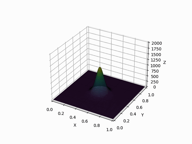
(b) $t=0.0003$

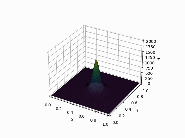
(c) $t=0.0006$

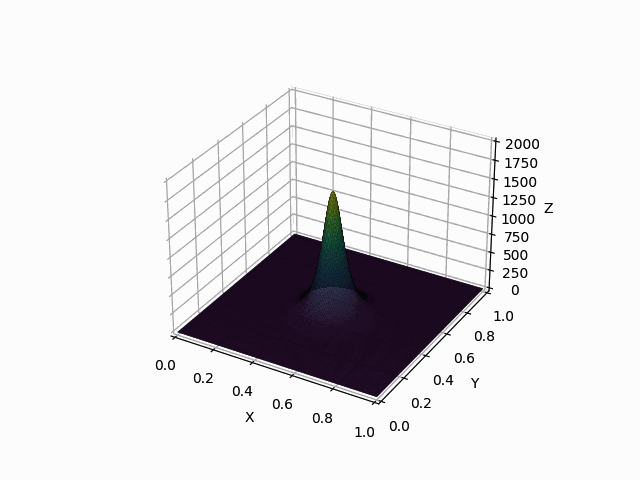
(d) $t=0.0009$

Figure 1: Simulation snapshots for $\rho_{h}$ with $k=1$ using $h=2^{-7.5}$ and $\tau=2^{-6}$ at different times.

Computing the full estimator results in overflows due to the exponential term. Thus, to validate the optimality of the error estimator, we perform experiments on the component estimators $\operatorname{E}_{0}$, $\operatorname{E}_{1}$, and $\operatorname{E}_{R_{\rho}}$ as well as the quantities $\bar{A}$ and $\bar{E}$ as specified in (70). As indicated in Tables 1 to 4, they show the expected EOCs. We observe that since the integrand $\bar{a}$ in $\bar{E}$ incorporates the broken $H^{1}$-norm of $\rho_{h}$, it is expected that the complete error estimator will be sensitive to the gradient of solution. Indeed, the full estimator behaves as expected, i.e. it converges with rate $k$ as long as the exact solution is smooth and round-off errors do not dominate.

$i$	$\bar{a}$	$E_{0}[\rho_{h}(0,\cdot)]$	EOC
$4$	6.86E+05	3.95E+02	2.017
$5$	1.59E+05	9.77E+01	2.008
$6$	3.99E+04	2.43E+01	2.003
$7$	1.22E+04	6.06E+00	2.001
$8$	5.48E+03	1.51E+00	2.000
$9$	3.83E+03	3.78E-01	-

Table 1: Tests were conducted for $\bar{a}$ and $E_{0}[\rho_{h}(0,\cdot)]$ using different values of $i$, with $k=1$. Note that the integrand $\bar{a}$ in $\bar{E}$ incorporates the broken $H^{1}$-norm of $\rho_{h}$, which is expected to be similar to the $H^{1}$-norm of $\rho$. The EOC for $E_{0}[\rho_{h}(0,\cdot)]$ matches the theoretical order.

$i$	$\bar{a}$	$E_{0}[\rho_{h}(0,\cdot)]$	EOC
$4$	7.03E+04	1.11E+02	3.025
$5$	7.33E+03	1.36E+01	2.946
$6$	3.54E+03	1.77E+00	2.955
$7$	3.31E+03	2.28E-01	2.974
$8$	3.29E+03	2.91E-02	-

Table 2: Tests were conducted for $\bar{a}$ and $E_{0}[\rho_{h}(0,\cdot)]$ using different values of $i$, with $k=2$. Note that the integrand $\bar{a}$ in $\bar{E}$ incorporates the broken $H^{1}$-norm of $\rho_{h}$, which is expected to be similar to the $H^{1}$-norm of $\rho$. The EOC for $E_{0}[\rho_{h}(0,\cdot)]$ matches the theoretical order.

$i$	$\left\|\operatorname{E}_{0}\right\|_{L^{\infty}(0,T)}$	EOC	$\left\|\operatorname{E}_{1}\right\|_{L^{2}(0,T)}$	EOC	$\left\|\operatorname{E}_{R_{\rho}}\right\|_{L^{2}(0,T)}$	EOC
$4$	4.30E+02	1.989	5.23E+01	1.068	4.37E+04	2.154
$5$	1.08E+02	2.002	2.50E+01	1.042	9.81E+03	1.544
$6$	2.70E+01	2.001	1.21E+01	1.021	3.37E+03	1.182
$7$	6.75E+00	2.000	5.97E+00	1.011	1.48E+03	1.055
$8$	1.69E+00	2.000	2.96E+00	1.005	7.14E+02	1.019
$9$	4.22E-01	-	1.48E+00	-	3.52E+02	-

Table 3: Polynomial degree $k=1$. Experimental results for $E_{0}[\rho_{h}(t,\cdot)]$, $E_{1}[\rho_{h}(t,\cdot)]$, $E_{R_{\rho}}[\rho_{h}(t,\cdot)]$. The sequence of solutions is computed with a mesh size $h=2^{1/2-i}$, time step $\tau=2^{2-i}$ and $T=0.0001$.

$i$	$\left\|\operatorname{E}_{0}\right\|_{L^{\infty}(0,T)}$	EOC	$\left\|\operatorname{E}_{1}\right\|_{L^{2}(0,T)}$	EOC	$\left\|\operatorname{E}_{R_{\rho}}\right\|_{L^{2}(0,T)}$	EOC
$4$	1.47E+02	2.988	1.64E+01	2.028	5.83E+03	3.042
$5$	1.85E+01	3.016	4.02E+00	2.024	7.08E+02	2.243
$6$	2.29E+00	3.005	9.88E-01	2.018	1.50E+02	2.074
$7$	2.85E-01	3.001	2.44E-01	2.009	3.55E+01	1.728
$8$	3.56E-02	-	6.06E-02	-	1.07E+01	-

Table 4: Polynomial degree $k=2$. Experimental results on $E_{0}[\rho_{h}(t,\cdot)]$, $E_{1}[\rho_{h}(t,\cdot)]$, $E_{R_{\rho}}[\rho_{h}(t,\cdot)]$. The sequence of solutions is computed with a mesh size $h=2^{1/2-i}$, time step $\tau=2^{2-i}$ and $T=0.0001$.

Remark 8.2.

We should note that due to the precision limitations of the float64 data type in the NumPy library, the $L^{2}$ norm of the jump of $c_{h}$ cannot decrease below a certain threshold. Consequently, the estimator $\tilde{E}_{1}[c_{h},\rho_{h}]$ and thus $E_{R_{\rho}}$ exhibit a deterioration of the EOC for $k=2$ beyond a certain refinement level as round-off errors start to dominate, see Table 5. Indeed, the squared jump of $c_{h}$ is bounded from below by $10^{-16}$, corresponding to the machine epsilon for float64 in NumPy, i.e. $2.22\times 10^{-16}$.

$i$	$\left\|\operatorname{\tilde{E}}_{1}\right\|_{L^{2}(0,T)}$	EOC
$4$	3.31E-02	2.071
$5$	7.87E-03	2.041
$6$	1.91E-03	2.019
$7$	4.72E-04	1.696
$8$	1.46E-04	-

Table 5: Polynomial degree $k=2$. Experimental results on $\tilde{E}_{1}[c_{h}(t,\cdot)]$. The sequence of solutions is computed with a mesh size $h=2^{1/2-i}$, time step $\tau=2^{2-i}$ and $T=0.0001$. The table shows that the EOC of $\tilde{E}_{1}[c_{h}(t,\cdot)]$ deteriorates at $i=8$.

Statements and Declarations

Conflict of interest

The authors declare no competing interests.

References

• [1] S. Bartels. Numerical Methods for Nonlinear Partial Differential Equations. Springer, 2015.
• [2] R. Becker and R. Rannacher. An optimal control approach to a posteriori error estimation in finite element methods. Acta Numerica, 10:1–102, may 2001. doi:10.1017/s0962492901000010.
• [3] P. Biler. Existence and asymptotics of solutions for a parabolic-elliptic system with nonlinear no-flux boundary conditions. Nonlinear Analysis. Theory, Methods & Applications. An International Multidisciplinary Journal, 19(12):1121–1136, 1992. doi:10.1016/0362-546X(92)90186-I.
• [4] P. Biler. Local and global solvability of some parabolic systems modelling chemotaxis. Advances in Mathematical Sciences and Applications, 8(2):715–743, 1998.
• [5] P. Biler and T. Nadzieja. Existence and nonexistence of solutions for a model of gravitational interaction of particles. I. Colloquium Mathematicum, 66(2):319–334, 1994. doi:10.4064/cm-66-2-319-334.
• [6] A. Blanchet, J. Dolbeault, and B. Perthame. Two-dimensional Keller-Segel model: optimal critical mass and qualitative properties of the solutions. Electronic Journal of Differential Equations, pages No. 44, 32, 2006.
• [7] C. J. Budd, R. Carretero-González, and R. D. Russell. Precise computations of chemotactic collapse using moving mesh methods. Journal of Computational Physics, 202(2):463–487, 2005. doi:10.1016/j.jcp.2004.07.010.
• [8] A. Cangiani, E. H. Georgoulis, I. Kyza, and S. Metcalfe. Adaptivity and blow-up detection for nonlinear evolution problems. SIAM Journal on Scientific Computing, 38(6):A3833–A3856, jan 2016. doi:10.1137/16M106073X.
• [9] A. Chertock and A. Kurganov. A second-order positivity preserving central-upwind scheme for chemotaxis and haptotaxis models. Numerische Mathematik, 111(2):169–205, 2008. doi:10.1007/s00211-008-0188-0.
• [10] A. Chertock, A. Kurganov, M. Ricchiuto, and T. Wu. Adaptive moving mesh upwind scheme for the two-species chemotaxis model. Computers & Mathematics with Applications. An International Journal, 77(12):3172–3185, 2019. doi:10.1016/j.camwa.2019.01.021.
• [11] Y. Epshteyn and A. Kurganov. New interior penalty discontinuous Galerkin methods for the Keller-Segel chemotaxis model. SIAM Journal on Numerical Analysis, 47(1):386–408, 2008/09. doi:10.1137/07070423X.
• [12] F. Filbet. A finite volume scheme for the Patlak-Keller-Segel chemotaxis model. Numerische Mathematik, 104(4):457–488, 2006. doi:10.1007/s00211-006-0024-3.
• [13] H. Gajewski, K. Zacharias, and K. Gröger. Global behaviour of a reaction-diffusion system modelling chemotaxis. Mathematische Nachrichten, 195(1):77–114, 1998. doi:10.1002/mana.19981950106.
• [14] J. Giesselmann and N. Kolbe. A posteriori error analysis of a positivity preserving scheme for the power-law diffusion keller-segel model, 2023. doi:10.48550/arXiv.2309.07329.
• [15] P. Grisvard. Singularities in Boundary Value Problems. Recherches en mathématiques appliquées. Masson, 1992. URL: https://books.google.co.kr/books?id=Kjqj-bAx4PYC.
• [16] L. Guo, X. H. Li, and Y. Yang. Energy dissipative local discontinuous Galerkin methods for Keller-Segel chemotaxis model. Journal of Scientific Computing, 78(3):1387–1404, 2019. doi:10.1007/s10915-018-0813-8.
• [17] T. Hillen and K. J. Painter. A user’s guide to PDE models for chemotaxis. Journal of Mathematical Biology, 58(1-2):183–217, jul 2008. doi:10.1007/s00285-008-0201-3.
• [18] D. Horstmann. From 1970 until present: the Keller-Segel model in chemotaxis and its consequences. I. Jahresbericht der Deutschen Mathematiker-Vereinigung, 105(3):103–165, 2003.
• [19] D. Horstmann. From 1970 until present: the Keller-Segel model in chemotaxis and its consequences. II. Jahresbericht der Deutschen Mathematiker-Vereinigung, 106(2):51–69, 2004.
• [20] D. Horstmann. Generalizing the keller–segel model: Lyapunov functionals, steady state analysis, and blow-up results for multi-species chemotaxis models in the presence of attraction and repulsion between competitive interacting species. Journal of Nonlinear Science, 21(2):231–270, nov 2010. doi:10.1007/s00332-010-9082-x.
• [21] O. A. Karakashian and F. Pascal. A posteriori error estimates for a discontinuous galerkin approximation of second-order elliptic problems. SIAM Journal on Numerical Analysis, 41(6):2374–2399, jan 2003. doi:10.1137/S0036142902405217.
• [22] D. Karmakar and G. Wolansky. On the critical mass patlak-keller-segel system for multi-species populations: global existence and infinite time aggregation, 2020. doi:10.48550/ARXIV.2004.10132.
• [23] E. F. Keller and L. A. Segel. Initiation of slime mold aggregation viewed as an instability. Journal of Theoretical Biology, 26(3):399–415, mar 1970. doi:10.1016/0022-5193(70)90092-5.
• [24] C. Kreuzer, C. A. Moller, A. Schmidt, and K. G. Siebert. Design and convergence analysis for an adaptive discretization of the heat equation. IMA Journal of Numerical Analysis, 32(4):1375–1403, jan 2012. doi:10.1093/imanum/drr026.
• [25] I. Kyza and S. Metcalfe. Pointwise a posteriori error bounds for blow-up in the semilinear heat equation. SIAM Journal on Numerical Analysis, 58(5):2609–2631, jan 2020. doi:10.1137/19M1264758.
• [26] X. H. Li, C.-W. Shu, and Y. Yang. Local discontinuous Galerkin method for the Keller-Segel chemotaxis model. Journal of Scientific Computing, 73(2-3):943–967, 2017. doi:10.1007/s10915-016-0354-y.
• [27] C. Makridakis. Space and time reconstructions in a posteriori analysis of evolution problems. In ESAIM Proceedings. Vol. 21 (2007) [Journées d’Analyse Fonctionnelle et Numérique en l’honneur de Michel Crouzeix], volume 21 of ESAIM Proc., pages 31–44. EDP Sci., Les Ulis, 2007. doi:10.1051/proc:072104.
• [28] C. Makridakis and R. H. Nochetto. Elliptic reconstruction and a posteriori error estimates for parabolic problems. SIAM Journal on Numerical Analysis, 41(4):1585–1594, 2003. doi:10.1137/s0036142902406314.
• [29] M. Mizuguchi, K. Tanaka, K. Sekine, and S. Oishi. Estimation of sobolev embedding constant on a domain dividable into bounded convex domains. Journal of Inequalities and Applications, 2017(1), nov 2017. doi:10.1186/s13660-017-1571-0.
• [30] J. D. Murray. Mathematical Biology I. An Introduction. Springer, 2002.
• [31] T. Nagai. Blow-up of radially symmetric solutions to a chemotaxis system. Advances in Mathematical Sciences and Applications, 5(2):581–601, 1995.
• [32] L. E. Payne and H. F. Weinberger. An optimal poincaré inequality for convex domains. Archive for Rational Mechanics and Analysis, 5(1):286–292, jan 1960. doi:10.1007/bf00252910.
• [33] D. A. D. Pietro and A. Ern. Mathematical Aspects of Discontinuous Galerkin Methods. Springer Berlin Heidelberg, 2012. doi:10.1007/978-3-642-22980-0.
• [34] C. Qiu, Q. Liu, and J. Yan. Third order positivity-preserving direct discontinuous galerkin method with interface correction for chemotaxis keller-segel equations. Journal of Computational Physics, 433:110191, may 2021. doi:10.1016/j.jcp.2021.110191.
• [35] N. Saito. Conservative upwind finite-element method for a simplified keller–segel system modelling chemotaxis. IMA Journal of Numerical Analysis, 27(2):332–365, apr 2007. doi:10.1093/imanum/drl018.
• [36] R. Strehl, A. Sokolov, D. Kuzmin, D. Horstmann, and S. Turek. A positivity-preserving finite element method for chemotaxis problems in 3D. Journal of Computational and Applied Mathematics, 239:290–303, 2013. doi:10.1016/j.cam.2012.09.041.
• [37] M. Sulman and T. Nguyen. A positivity preserving moving mesh finite element method for the keller–segel chemotaxis model. Journal of Scientific Computing, 80(1):649–666, mar 2019. doi:10.1007/s10915-019-00951-0.
• [38] T. Suzuki. Free Energy and Self-Interacting Particles (Progress in Nonlinear Differential Equations and Their Applications). Birkhäuser Boston, 2005.
• [39] R. Tyson, L. G. Stern, and R. J. LeVeque. Fractional step methods applied to a chemotaxis model. Journal of Mathematical Biology, 41:455–475, 2000. doi:10.1007/s002850000038.
• [40] T. Warburton and J. Hesthaven. On the constants in hp-finite element trace inverse inequalities. Computer Methods in Applied Mechanics and Engineering, 192(25):2765–2773, jun 2003. doi:10.1016/s0045-7825(03)00294-9.
• [41] G. Wolansky. Multi-components chemotactic system in the absence of conflicts. European Journal of Applied Mathematics, 13(6):641–661, 2002. doi:10.1017/S0956792501004843.