A Robust Finite-Difference Model Reduction for the Boundary Feedback Stabilization of Fully-dynamic Piezoelectric Beams

Abstract

Piezoelectric materials exhibit electric responses to mechanical stress, and mechanical responses to electric stress. The PDE model, describing the longitudinal oscillations on the beam, with two boundary feedback controllers is known to have exponentially stable solutions. However, the reduced model by the semi-discretized Finite Elements is shown to lack of exponential stability uniformly as the discretization parameter tends to zero. This is due to the loss of uniform gap among the high-frequency eigenvalues. In this paper, an alternate Finite-Difference based model reduction is investigated by cleverly reducing the order of the model together with the consideration of equidistant grid points and averaging operators. This new model reduction successfully retains the exponential stability uniformly as the discretization parameter tends to zero. Moreover, it does not need a further numerical Fourier filtering. Our results are based on a careful construction of a Lyapunov function. The numerical simulations are provided to compare reduced models and to show the strength of introduced results.

piezoelectric beams, exponential stabilization, optimal feedback gains, order-reduction, Fourier filtering, maximal decay rate

1 Introduction

A piezoelectric material, such as lead zirconate titanate (PZT), barium titanate or lead titanate, is a multi-functional smart material to develop electric displacement, directly proportional to an applied mechanical stress [40]. These materials can be used for designing actuators requiring an electrical input (current, charge or voltage) [30, 28, 45]. One of the main components of the electrical input is the drive frequency which determines how fast a piezoelectric beam vibrates or changes its state. Periodic and arbitrary signals can be used to drive a piezoelectric beam, which corresponds to continuous control of vibrational modes. both high resolution and high bandwidth. Piezoelectric actuators can achieve positioning resolution down to tens of nanometers. Piezoelectric materials are also used as sensors or energy harvesters, i.e. see [2].

For many applications of piezoelectricity, electrostatic/quasi-static approximations due to Maxwell’s equations are sufficient to describe low-frequency vibrations since magnetic effects are fully/partially discarded. However, i.e. for piezoelectric acoustic wave devices, magnetic effects may become more dominant, and therefore, the system equations of the existing models in the literature can not recover the real vibrational dynamics on these devices. Indeed, more accurate models incorporating the electromagnetic and mechanical interactions are needed, i.e. see [7, 41] and the references therein. Note that as electromagnetic waves are involved, unlike the electrostatic and electrostatic models, the full set of Maxwell equations are needed to be coupled to the equations due to mechanical vibrations [40, 21, 30]. Such a fully-dynamic theory has been called piezo-electro-magnetism by some researchers [45].

Consider a beam of piezoelectric material, clamped on one side and free to oscillate on the other, with the addition of a controller for the tip velocity and tip current accumulated at the electrodes of the beam. The beam is of length $L.$ Assume that the transverse oscillations of the beam are negligible, so the longitudinal oscillations, in the form of expansion and compression of the center line of the beam, are the only oscillations of note.

Define the following positive-definite matrices

$$C_{1}=\begin{bmatrix}\rho&0\\ 0&\mu\\ \end{bmatrix},C_{2}=\begin{bmatrix}\alpha&-\gamma\beta\\ -\gamma\beta&\beta\\ \end{bmatrix},C_{3}=\begin{bmatrix}k_{1}&0\\ 0&k_{2}\\ \end{bmatrix},$$

where $k_{1},k_{2}>0$ are state feedback gains, and $\rho$, $\alpha$ (and $\alpha_{1}$), $\beta$, $\gamma$, and $\mu$ are all piezoelectric material-specific positive constants, namely, the mass density per unit volume, the elastic and piezoelectric stiffness, the beam coefficient of impermeability, the piezoelectric constant, and the magnetic permeability. Moreover, $\alpha_{1}=\alpha-\gamma^{2}\beta.$

Denoting dots $``\cdot"$ by the derivatives with respect to the time variable $t$, $v(x,t)$ and $p(x,t)$ by the longitudinal oscillations of the center line of the beam and the total charge accumulated at the electrodes of the beam, respectively, the equations of motion is a system of strongly-coupled equations

$$\left\{\begin{array}[]{ll}C_{1}\begin{bmatrix}\ddot{v}\\ \ddot{p}\\ \end{bmatrix}+C_{2}\begin{bmatrix}v_{xx}\\ p_{xx}\\ \end{bmatrix}=0,&\\ \begin{bmatrix}v\\ p\\ \end{bmatrix}(0,t)=0,&\\ \left(C_{2}\begin{bmatrix}v_{x}\\ p_{x}\\ \end{bmatrix}+C_{3}\begin{bmatrix}\dot{v}\\ \dot{p}\\ \end{bmatrix}\right)(L,t)=0,\quad t\in\mathbb{R}^{+}&\\ \left[v,p,\dot{v},\dot{p}\right]\left(x,0\right)=\left[v_{0},p_{0},v_{1},p_{1}\right]\left(x\right),x\in\left[0,L\right].\end{array}\right.$$ (5)

The natural energy of the solutions of (5) is defined as

$$\begin{array}[]{ll}E(t)=\frac{1}{2}\int^{L}_{0}\left\{C_{1}\begin{bmatrix}\dot{v}\\ \dot{p}\\ \end{bmatrix}\cdot\begin{bmatrix}\dot{v}\\ \dot{p}\\ \end{bmatrix}+C_{2}\begin{bmatrix}v_{x}\\ p_{x}\\ \end{bmatrix}\cdot\begin{bmatrix}v_{x}\\ p_{x}\\ \end{bmatrix}\right\}~{}dx.\end{array}$$ (7)

1.1 Related Literature on the PDE Model

The system (5) with only one state feedback controller, $k_{1}=0,k_{2}\neq 0$ or $k_{1}\neq 0,k_{2}=0$, is shown to lack of exponential stability/exact controllability. Moreover, for certain combinations of the material constants, even approximate controllability/strong stability is at stake [21]. These combinations are mostly corresponding to the high-frequency electromagnetic vibrations. Indeed, by a deeper investigation in [22], an exponential stability is obtained in a more regular state space and with a slim class of material parameters. Indeed, two feedback controllers, $k_{1},k_{2}\neq 0,$ is a necessity to make the system exponentially stable without any restriction on the material parameters. Indeed, the exponential stability of the solutions of the controlled system (5) with $k_{1},k_{2}\neq 0$ is shown in [38] by a decomposition argument together with an observability inequality with a suboptimal observation time. Unfortunately, this approach prevents finding the optimal feedback gains to achieve the maximal decay rate. Their result is improved by a strategically-constructed Lyapunov function with which the maximal decay rate together with the optimal feedback gains are provided explicitly [24]. The proof of the result below does not need an observability inequality.

Noting that $\sqrt{\frac{\rho}{\alpha_{1}}}$ and $\sqrt{\frac{\beta}{\mu}}$ are non-identical wave propagation speeds of the wave equations in (5), define the maximum of the group speeds, due to strong coupling, by

$$\begin{array}[]{ll}\quad\eta:=\max\left(\sqrt{\frac{\rho}{\alpha_{1}}}+\sqrt{\frac{\mu\gamma^{2}}{\alpha_{1}}},\sqrt{\frac{\mu}{\beta}}+\sqrt{\frac{\mu\gamma^{2}}{\alpha_{1}}}\right),\end{array}$$ (9)

and the Hilbert space $\mathcal{H}:=(H^{1}_{*}(0,L))^{2}\times(L^{2}(0,L))^{2}$ where $(H^{1}_{*}(0,L))=\{z\in H^{1}(0,L):z(0)=0\}.$

Theorem 1

[24, Theorem 4] The energy $E(t)$ is dissipative, i.e., $\frac{dE}{dt}=-k_{1}\left|v_{t}(L,t)\right|^{2}-k_{2}\left|p_{t}(L,t)\right|^{2}\leq 0$ for all $t>0.$ Moreover, for any $\epsilon>0$ and $(v,p,\dot{v},\dot{p}),(v_{0},p_{0},v_{1},p_{1})\in\mathcal{H},$ the energy $E(t)$ decays exponentially, i.e.

$$\left\{\begin{array}[]{ll}E(t)\leq ME(0)e^{-\sigma t},\qquad\forall t>0\\ \sigma(\delta(\xi_{1},\xi_{2},\epsilon))=\delta\left(1-\delta L\eta\right),\\ M(\delta(\xi_{1},\xi_{2},\epsilon))=\frac{1+\delta L\eta}{1-\delta L\eta},\quad{\text{where}}\end{array}\right.$$ (13)

$$\left\{\begin{array}[]{ll}\delta(k_{1},k_{2},\epsilon):=\frac{1}{2L}\text{min}\left(\frac{1}{\eta},f_{1}(k_{2},\epsilon),f_{2}(k_{2},\epsilon)\right),\\ f_{1}(k_{1},\epsilon):=\frac{2k_{1}\alpha_{1}}{\rho\alpha_{1}+(1+\epsilon)k_{1}^{2}},\\ f_{2}(k_{2},\epsilon):=\frac{4k_{2}\epsilon\alpha_{1}\beta}{\epsilon\mu\alpha_{1}\beta+(\epsilon\alpha+\gamma^{2}\beta)k_{2}^{2}}.\end{array}\right.$$ (17)

Note that the decay rate $\sigma(\delta)$ is maximal as the system exponentially stabilizes fastest. It is straightforward that $\sigma(\delta(\xi_{1},\xi_{2},\epsilon))$ makes its maximal value

$$\sigma_{max}(\delta)=\frac{1}{4\eta L}~{}{\rm achieved~{}at}~{}\delta=\frac{1}{2\eta L}.$$ (18)

Since $\delta$ is a function of $k_{1},k_{2},\epsilon$, to achieve $\delta=\frac{1}{2\eta L},$ an optimization argument is needed to provides safe intervals for the feedback amplifiers $k_{1},k_{2}$ and $\epsilon$.

It is crucial to note that there are recently appeared results in the literature for (5) with passivity-based approach [8] or with different damping designs. In the case of distributed damping, the system can be stabilized exponentially by only one viscous damping [37], which is interestingly enough to stabilize the coupled dynamics. In the case of two delayed-type damping designs, the exponential stability is achieved for various combinations of boundary and distributed damping designs [10, 19] Fractional damping together with thermal effects are also considered for the nonlinear piezoelectric beam design. Indeed, the resulting model reduced to a single boundary-controlled wave equation [11], which is known to have exponentially stable solutions. Moreover, the system (5) is considered for the long-range boundary and distributed memory terms for exponential stability [9] and polynomial stability [46].

1.2 Related Literature on Model Reductions

For simulation and control purposes, a model reduction is required for the PDE model, e.g. by Finite Differences or Finite Elements. This results in a system of ordinary differential equations (ODE). In this case, the controller design for model reductions are implemented by the approximations of the one for PDE model. The control design based on a finite-dimensional model reduction may excite the unmodeled modes, leading to the so-called spillover effect [35]. Moreover, implementing some of the standard approximations results in spurious unobservable (high-frequency) vibrational modes in the approximated dynamics; see [47] for a detailed discussion. Therefore, the finite dimensional model reductions do not retain exact observability uniformly as the discretization parameter approaches zero. These unobservable spurious high-frequency modes are eliminated by, i.e. the “direct Fourier filtering” or “indirect filtering” methods [13]. The Direct Fourier filtering is shown to be more efficient than the indirect filtering since it encompasses both low and high-frequency eigenvalues, while ignoring spurious eigenvalues. In fact, the direct Fourier filtering is successfully applied by a decomposition approach [13, 6] and by a direct Lyapunov approach [24] for the single wave equation, for the Euler-Bernoulli beam [15], Rayleigh beam [29], and a multi-layer beam model [31, 33]. A standard Finite Difference-based model reduction for the boundary observation of the system (5), $k_{1},k_{2}\equiv 0,$ is proposed for the first time in [32]. The number of eigenvalues of two distinct branches are filtered identically via the direct Fourier filtering technique. Therefore, the uniform observability result is retained as the discretization parameter tends to zero. The same model reduction is shown to lack exponential stability as the discretization parameter tends to zero yet the implementation of the direct Fourier filtering adds stringent conditions in the exponential stability result [25]. On another note, the major drawback of the direct Fourier filtering is the vagueness of the optimality of the applied filtering [20]. Recently, a novel Finite Differences-based model reduction is proposed for the wave equation [17] and the Euler-Bernoulli beam model [16, 18]. The reduced model is constructed using equidistant grid points and averaging operators, and thus, a numerical filtering is completely avoided. The uniform observability result is proved directly by the discrete multipliers method.

1.3 Our Contributions and Content

In this paper, (i) first, a Finite Elements-based model reduction of the system (5) with linear splines is proposed for the first time. (ii) It is shown that this model lacks exponential stability as the discretization parameter tends to zero, without proper numerical filtering. With filtering, this model is proposed as a robust model reduction for the system (5). (iii) Adopting the order-reduction strategy in [16]-[18], a robust Finite-Difference based model reduction for (5) is proposed. This way, the need of numerical Fourier filtering is completely discarded. (iv) Once the exponential stability of the reduced model is established by a clever use of a Lyapunov theory, the convergence of the energy is also proved as the discretization parameter tends to zero. To the best of our knowledge, this method is never investigated for a strongly coupled system such as (5). Our results not only extend the results in [32, 38] but provide better insights to understand the overall exponential stability of the reduced models of strongly-coupled systems of wave equations such as [27, 28, 30].

2 A Model Reduction by Finite Elements Method (FEM) with Linear Splines

To find a reduced model corresponding to (5), one may use the Finite Elements. Letting $N\in\mathbb{N}$ be given, and defining the mesh size $h:=\frac{1}{N+1}$, consider a uniform discretization of the interval $[0,L]$:

$$0=x_{0}<x_{1}<...<x_{i}=i*h<\ldots<x_{N+1}=L.$$ (19)

First, multiply both sides of the equation in (5) by a continuously differentiable test function $\vec{\phi}(x)=\begin{bmatrix}\phi^{1}(x)\\ \phi^{2}(x)\\ \end{bmatrix}\in(C_{0}^{\infty}[0,L])^{2}$, and integrate both sides of the equation over $[0,L]$ to obtain the following weak formulation

$$\begin{array}[]{ll}C_{1}\begin{bmatrix}\ddot{v}\\ \ddot{p}\\ \end{bmatrix}\cdot\begin{bmatrix}\phi^{1}\\ \phi^{2}\\ \end{bmatrix}-C_{2}\begin{bmatrix}v_{x}\\ p_{x}\\ \end{bmatrix}\cdot\begin{bmatrix}\phi^{1}_{x}\\ \phi^{2}_{x}\\ \end{bmatrix}&\\ \qquad\qquad\qquad\qquad\qquad+C_{3}\begin{bmatrix}\dot{v}\\ \dot{p}\\ \end{bmatrix}\cdot\begin{bmatrix}\phi^{1}\\ \phi^{2}\\ \end{bmatrix}(L)=\vec{0}.\end{array}$$ (22)

For each $j=1,2$, and at each node $\left\{x_{i}\right\}_{i=1}^{N}$, linear splines are defined as the following

$$\phi_{i}^{j}(x)=\left\{\begin{array}[]{ll}\frac{1}{h}(x-x_{i}),&x_{i-1}<x<x_{i}\\ \frac{1}{h}(x-x_{i+1}),&x_{i}<x<x_{i+1}\\ 0,&{\textrm{o}therwise}\end{array}\right.$$ (26)

$$\phi^{j}_{N+1}(x)=\left\{\begin{array}[]{ll}\frac{1}{h}(x-x_{N}),&x_{N}<x<x_{N+1}\\ 0,&{\textrm{o}therwise}\end{array}\right.$$ (29)

Define the $(N+1)\times(N+1)$ matrix $M$ by

$$M:=\left(\begin{array}[]{cccccc}2/3&1/6&0&0&\ldots&0\\ 1/6&2/3&1/6&0&\ldots&0\\ \vdots&\vdots&\ddots&\ddots&\ddots&\vdots\\ 0&0&0&1/6&2/3&1/6\\ 0&0&\ldots&0&1/6&1/3\\ \end{array}\right).$$ (35)

Moreover, consider the central differences for $v_{xx}(x_{j})\approx(-A_{h}\vec{v})_{j}$ and $p_{xx}(x_{j})\approx(-A_{h}\vec{p})_{j}$ with the $(N+1)\times(N+1)$ matrix $A_{h}$ defined by

$$A_{h}=\frac{1}{h^{2}}\begin{bmatrix}2&-1&0&\dots&\dots&\dots&0\\ -1&2&-1&0&\dots&\dots&0\\ &\ddots&\ddots&\ddots&\ddots&\ddots&\\ 0&\dots&\dots&0&-1&2&-1\\ 0&\dots&\dots&\dots&0&-1&1\\ \end{bmatrix}.$$ (36)

Now, letting $B:=\begin{bmatrix}0&0&\dots&0\\ 0&0&\dots&0\\ \vdots&\ddots&\ddots&\vdots&\\ 0&\dots&0&1\\ \end{bmatrix},$ the weak formulation (22) is reduced to

$$\left\{\begin{array}[]{ll}(C_{1}\bigotimes M)\begin{bmatrix}{\ddot{\vec{v}}}\\ {\ddot{\vec{p}}}\\ \end{bmatrix}+\left(C_{2}\bigotimes A_{h}\right)\begin{bmatrix}{{\vec{v}}}\\ {{\vec{p}}}\\ \end{bmatrix}&\\ \qquad+(C_{3}\bigotimes B)\begin{bmatrix}{\dot{\vec{v}}}\\ {\dot{\vec{p}}}\\ \end{bmatrix}=\vec{0},\quad t\in\mathbb{R}^{+},&\end{array}\right.$$ (39)

where $\bigotimes$ is the Kronecker product. Indeed, the system (39) can be simplified further by the mixed-product property of the Kronecker product as the following

$$\left\{\begin{array}[]{ll}\begin{bmatrix}{\ddot{\vec{v}}}\\ {\ddot{\vec{p}}}\\ \end{bmatrix}+\left(C_{1}^{-1}C_{2}\right)\bigotimes\left(M^{-1}A_{h}\right)\begin{bmatrix}{{\vec{v}}}\\ {{\vec{p}}}\\ \end{bmatrix}&\\ \qquad+\left((C_{1}^{-1}C_{3}\right)\bigotimes\left(M^{-1}B\right)\begin{bmatrix}{\dot{\vec{v}}}\\ {\dot{\vec{p}}}\\ \end{bmatrix}=\vec{0},\quad t\in\mathbb{R}^{+}&\\ (v,\dot{v})_{k}(0)=(v^{0},v^{1})(x_{k}),&\\ (p,\dot{p})_{k}(0)=(p^{0},p^{1})(x_{k}),~{}~{}k=0,...,N+1,\end{array}\right.$$ (44)

Note that the eigenvalues of the matrix is analytically represented in the following result

Theorem 2

[23, Lemma 3] For $j,k=1,\ldots,N+1,$ the eigenvalues of $M^{-1}A_{h}$ are given by

$$\begin{array}[]{ll}{\lambda}_{k}(M^{-1}A_{h})&=\frac{\lambda_{k}(A_{h})}{1-\frac{h^{2}}{6}\lambda_{k}(A_{h})}=\frac{1}{h^{2}}\frac{6-6\cos{\left(\frac{(2k-1)\pi h}{2(L-h)}\right)}}{2+\cos{\left(\frac{(2k-1)\pi h}{2(L-h)}\right)}}.\end{array}$$ (46)

Moreover, $\lambda_{k}(M^{-1}A_{h})h^{2}<12$ for all $h>0,$ and $\lambda_{k}(A_{h})\to\frac{\pi^{2}(2k-1)^{2}}{L^{2}}$ for fixed $k$ and $\lambda_{N}(M^{-1}A_{h})h^{2}\to 12$ as $h\to 0.$

Let $Z_{h}=\frac{1}{h}{\rm tridiag}(0,-1,1)$ be an $(N+1)\times(N+1)$ tridiagonal matrix. The discretized energy corresponding to (44), the discretized counterpart of (7), is

$$\begin{array}[]{ll}&E_{h}^{\rm FEM}(t):=\frac{h}{2}\left\{(C_{1}\bigotimes M)\begin{bmatrix}{\dot{\vec{v}}}\\ {\dot{\vec{p}}}\\ \end{bmatrix}\right\}\cdot\begin{bmatrix}{\dot{\vec{v}}}\\ {\dot{\vec{p}}}\\ \end{bmatrix}\\ &+\frac{h}{2}\left\{(C_{2}\bigotimes Z_{h})\begin{bmatrix}{{\vec{v}}}\\ {{\vec{p}}}\\ \end{bmatrix}\right\}\cdot\left\{(I\bigotimes Z_{h})\begin{bmatrix}{{\vec{v}}}\\ {{\vec{p}}}\\ \end{bmatrix}\right\}\\ &+\frac{h}{12}\left(C_{1}\begin{bmatrix}{\dot{v}}_{N+1}\\ {\dot{p}}_{N+1}\\ \end{bmatrix}\cdot\begin{bmatrix}{\dot{v}}_{N+1}\\ {\dot{p}}_{N+1}\\ \end{bmatrix}+6C_{2}\begin{bmatrix}{{v}}_{N+1}\\ {{p}}_{N+1}\\ \end{bmatrix}\cdot\begin{bmatrix}{{v}}_{N+1}\\ {{p}}_{N+1}\\ \end{bmatrix}\right).\end{array}$$

2.1 Spectral Analysis and Fourier Solutions

Consider the control-free system, i.e. (44) with $C_{3}\equiv 0.$ Let $\{\phi_{j}\}_{j=1}^{4}\in\mathbb{C}^{N}$ , and let $\vec{\phi}=[\phi_{1},\phi_{2},\phi_{3},\phi_{4}]^{\rm T}.$ Now we rewrite (44) as the following

$$\left\{\begin{array}[]{ll}&\dot{\vec{\phi}}=\tilde{\mathcal{A}}^{\rm FEM}\vec{\phi}=:\left({\begin{array}[]{*{20}c}0&I\\ A&0\end{array}}\right)\vec{\phi},\\ &\vec{\phi}(0)=\vec{\phi}_{0},\end{array}\right.$$ (52)

where $A_{(2N+2)\times(2N+2)}=-\left(C_{1}^{-1}C_{2}\right)\bigotimes\left(M^{-1}A_{h}\right)$. Next, consider the eigenvalue problem

$${\tilde{\mathcal{A}}}^{\rm FEM}\left(\begin{array}[]{c}{\vec{\psi}}^{1}\\ {\vec{\psi}}^{2}\end{array}\right)={{\tilde{\lambda}}}(h)\left(\begin{array}[]{c}{\vec{\psi}}^{1}\\ {\vec{\psi}}^{2}\end{array}\right)$$ (57)

Define the following constants

$$\begin{array}[]{ll}\zeta_{1}:=\frac{1}{\sqrt{2}}\sqrt{\frac{\alpha}{\rho}+\frac{\beta}{\mu}+\sqrt{\left(\frac{\alpha}{\rho}+\frac{\beta}{\mu}\right)^{2}-\frac{4\alpha_{1}}{\mu\rho}}},&\\ \zeta_{2}:=\frac{1}{\sqrt{2}}\sqrt{\frac{\alpha}{\rho}+\frac{\beta}{\mu}-\sqrt{\left(\frac{\alpha}{\rho}+\frac{\beta}{\mu}\right)^{2}-\frac{4\alpha_{1}}{\mu\rho}}},&\\ b_{1}:=\frac{1}{\gamma\mu}(\frac{\alpha_{1}}{\zeta_{1}^{2}}-\rho),\quad b_{2}:=\frac{1}{\gamma\mu}(\frac{\alpha_{1}}{\zeta_{2}^{2}}-\rho)&\\ \end{array}$$ (61)

where $\zeta_{1},\zeta_{2}>0.$ As well, $b_{1},b_{2}\neq 0,$ $b_{1}\neq b_{2},$ and $b_{1}b_{2}=-\frac{\rho}{\mu}.$ Moreover, $b_{1}$ and $b_{2}$ satisfy the quadratic equation

$$b^{2}-\left(\frac{\alpha}{\gamma\beta}-\frac{\rho}{\gamma\mu}\right)b-\frac{\rho}{\mu}=0.$$ (62)

The Kronecker product has the property that the eigenvalues of the matrix $\left(C_{1}^{-1}C_{2}\right)\bigotimes\left(M^{-1}A_{h}\right)$ is the product of the eigenvalues of $\left(C_{1}^{-1}C_{2}\right)$ and the eigenvalues of $\left(M^{-1}A_{h}\right).$ Now, the eigenvalues of the matrix $\left(C_{1}^{-1}C_{2}\right)$ are easily calculated as $\{\zeta_{1}^{2},\zeta_{2}^{2}\}.$ Therefore, this together with (65), the following theorem, describing the spectrum of $\tilde{\mathcal{A}}^{\rm FEM},$ is immediate.

Theorem 3

Assume $C_{3}\equiv 0$ in (44). The matrix $\tilde{\mathcal{A}}^{\rm FEM}$ has two branches of eigenvalues

$$\left\{\begin{array}[]{ll}\tilde{\lambda}_{1k}^{\mp}(h)=\mp i\zeta_{1}\sqrt{{\lambda}_{k}(M^{-1}A_{h})},&\\ \tilde{\lambda}_{2k}^{\mp}(h)=\mp i\zeta_{2}\sqrt{{\lambda}_{k}(M^{-1}A_{h})},\end{array}\right.$$ (65)

and since $\tilde{\lambda}_{1k}^{-}=-\tilde{\lambda}_{1k}^{+},~{}~{}\tilde{\lambda}_{2k}^{-}=-\tilde{\lambda}_{2k}^{+},$ the corresponding eigenvectors are

$${\vec{\Psi}}^{1}_{k}(h)=\left(\begin{array}[]{c}\frac{1}{\tilde{\lambda}_{1k}^{+}}{\vec{\psi}}_{k}\\ \frac{b_{1}}{\tilde{\lambda}_{1k}^{+}}{\vec{\psi}}_{k}\\ {\vec{\psi}}_{k}\\ b_{1}{\vec{\psi}}_{k}\end{array}\right),~{}{\vec{\Psi}}^{-1}_{k}(h)=\left(\begin{array}[]{c}\frac{1}{\tilde{\lambda}_{1k}^{+}}{\vec{\psi}}_{k}\\ \frac{b_{1}}{\tilde{\lambda}_{1k}^{+}}{\vec{\psi}}_{k}\\ -{\vec{\psi}}_{k}\\ -b_{1}{\vec{\psi}}_{k}\end{array}\right),$$ (74)

$$~{}{\vec{\Psi}}^{2}_{k}(h)=\left(\begin{array}[]{c}\frac{1}{\tilde{\lambda}_{2k}^{+}}{\vec{\psi}}_{k}\\ \frac{b_{1}}{\tilde{\lambda}_{2k}^{+}}{\vec{\psi}}_{k}\\ {\vec{\psi}}_{k}\\ b_{2}{\vec{\psi}}_{k}\end{array}\right),~{}{\vec{\Psi}}^{-2}_{k}(h)=\left(\begin{array}[]{c}\frac{1}{\tilde{\lambda}_{2j}^{+}}{\vec{\psi}}_{k}\\ \frac{b_{2}}{\tilde{\lambda}_{2j}^{+}}{\vec{\psi}}_{k}\\ -{\vec{\psi}}_{k}\\ -b_{2}{\vec{\psi}}_{k}\end{array}\right).$$ (83)

where ${\psi}_{k,j}=sin\left(\frac{(2k-1)j\pi}{2N}\right),$ for $j,k=1,\ldots,N+1.$ For fixed $k,$

$$\lim\limits_{h\to 0}\sqrt{{\tilde{\lambda}}_{ik}(h)}=\frac{(2k-1)\pi}{2L}\zeta_{i},\quad i=1,2,\quad k=1,2,\ldots,N.$$

The solutions to (52) is given by

$$\begin{array}[]{ll}\varphi(x,t)=\sum\limits_{j=1}^{N}\left[c_{1j}{\vec{\Psi}}^{1}_{k}(h)e^{\tilde{\lambda}_{1j}^{+}t}+d_{1j}{\vec{\Psi}}^{-1}_{k}(h)e^{-\tilde{\lambda}_{1j}^{+}t}\right.&\\ \left.+c_{2j}{\vec{\Psi}}^{2}_{k}(h)e^{\tilde{\lambda}_{2j}^{+}t}+d_{2j}{\vec{\Psi}}^{-2}_{k}(h)e^{-\tilde{\lambda}_{2j}^{+}t}\right].\end{array}$$ (86)

for the initial data

$$\begin{array}[]{ll}\varphi^{0}=\sum\limits_{j=1}^{N}\left(\begin{array}[]{c}\frac{1}{\tilde{\lambda}_{1j}^{+}}(c_{1j}+d_{1j})+\frac{1}{\tilde{\lambda}_{2j}^{+}}(c_{2j}+d_{2j})\\ \frac{b_{1}}{\tilde{\lambda}_{1j}^{+}}(c_{1j}+d_{1j})+\frac{b_{2}}{\tilde{\lambda}_{2j}^{+}}(c_{2j}+d_{2j})\\ (c_{1j}-d_{1j})+(c_{2j}-d_{2j})\\ b_{1}(c_{1j}-d_{1j})+b_{2}(c_{2j}-d_{2j})\end{array}\right)\psi_{j}(h)\end{array}$$ (92)

where $\{c_{kj},d_{kj},\quad k=1,2,\quad j\in\mathbb{N}\}$ are complex numbers such that

$$\begin{array}[]{ll}\|\varphi^{0}\|_{\mathbb{R}^{N}}^{2}\asymp\sum\limits_{j=1}^{N}\left(|c_{1j}|^{2}+|d_{1j}|^{2}+|c_{2j}|^{2}+|d_{2j}|^{2}\right),{\rm i.e.}&\\ \tilde{C}_{1}~{}\|\varphi^{0}\|_{\mathbb{R}^{N}}^{2}\leq\sum\limits_{i=1}^{2}\sum\limits_{j=1}^{N}\left(|c_{ij}|^{2}+|d_{ij}|^{2}\right)\leq\tilde{C}_{2}~{}\|\varphi^{0}\|_{\mathbb{R}^{N}}^{2}\end{array}$$ (95)

with two positive constants $\tilde{C}_{1},\tilde{C}_{2}$ which are independent of the particular choice of $\varphi^{0}.$

2.2 Lack of Observability as $h\to 0$

The following lemma is needed for proving the main result.

Lemma 1

For any eigen-pair $\left[{\tilde{\lambda}}(h),\left(\begin{array}[]{c}{\vec{\psi}}^{1}\\ {\vec{\psi}}^{2}\end{array}\right)\right]$ of ${\tilde{\mathcal{A}}}^{\rm FEM}$, the following identities hold:

$$\begin{array}[]{ll}\alpha_{1}\sum\limits_{j=0}^{N+1}\left|\frac{\psi^{1}_{j+1}-\psi^{1}_{j}}{h}\right|^{2}+\beta\sum\limits_{j=0}^{N+1}\left|\frac{(\gamma\psi^{1}_{j+1}-\psi^{2}_{j+1})-(\gamma\psi^{1}_{j}-\psi^{2}_{j})}{h}\right|^{2}\\ \qquad={\lambda}_{k}(M^{-1}A_{h})\left(\sum\limits_{j=0}^{N+1}\rho|\psi^{1}_{j}|^{2}+\mu|\psi^{2}_{j}|^{2}\right),\end{array}$$ (98)

and

$$\begin{array}[]{ll}&\frac{{\lambda}_{k}(M^{-1}A_{h})(2L-h)}{2h}\left(\rho\left|\psi^{1}_{N+1}\right|^{2}\mu\left|\psi^{2}_{N+1}\right|^{2}\right)\\ &={\lambda}_{k}(M^{-1}A_{h})\left[2\rho\left(1-\frac{\rho{\lambda}_{k}(M^{-1}A_{h})h^{2}}{12\alpha_{1}}\right)\sum\limits_{j=0}^{N+1}(\psi^{1}_{j})^{2}\right.\\ &\quad+2\mu\left(1-\frac{\alpha\mu{\lambda}_{k}(M^{-1}A_{h})h^{2}}{12\beta\alpha_{1}}\right)\sum\limits_{j=0}^{N}(\psi^{2}_{j})^{2}\\ &\left.\quad-\frac{\rho\mu\gamma{\lambda}_{k}(M^{-1}A_{h})h^{2}}{\alpha_{1}}\sum\limits_{j=0}^{N+1}\psi^{1}_{j}\psi^{2}_{j}\right].\end{array}$$ (103)

Proof 2.1.

The proof follows the same exact steps of [32, Lemma 3.2] where the mass matrix $M$ is the identity matrix $I.$ Once ${\lambda}_{k}(A_{h})$ is replaced by ${\lambda}_{k}(M^{-1}A_{h}),$ (98) and (103) are immediate.

Theorem 4 (Lack of Observability).

Let $\xi_{1}=\xi_{2}\equiv 0$ in (52). For any $T>0,$ as $h\to 0$

$$\sup\limits_{\left(\begin{array}[]{c}{\vec{v}}\\ {\vec{p}}\end{array}\right)\ ~{}\rm solves~{}(\ref{disc})}\frac{E_{h}(0)}{\int_{0}^{T}\left\{C_{1}\begin{bmatrix}{\dot{v}}_{N+1}\\ {\dot{p}}_{N+1}\\ \end{bmatrix}\cdot\begin{bmatrix}{\dot{v}}_{N+1}\\ {\dot{p}}_{N+1}\\ \end{bmatrix}\right\}dt}\to\infty.$$ (106)

Proof 2.2.

Consider the solution $\left(\begin{array}[]{c}\vec{v}\\ \vec{p}\end{array}\right)=\left(\begin{array}[]{c}\vec{\psi}_{N+1}\\ b_{k}{\vec{\psi}}_{N+1}\end{array}\right)$ corresponding to the eigenvalue

$$\tilde{\lambda}_{N+1}(h)=i\zeta_{k}\sqrt{{\lambda}_{N+1}(M^{-1}A_{h})}$$

where $k=1$ or $k=2.$ By the normalization $h\sum\limits_{j=0}^{N+1}(\psi_{N+1,j})^{2}=1,$ (103) yields

$$\begin{array}[]{ll}&\tilde{\lambda}_{N+1}(h)\frac{(2L-h)}{2}\left|\psi_{N+1,N+1}\right|^{2}\\ &=E_{h}(0)\left[2\rho\left(\frac{12\alpha_{1}(\zeta_{k})^{2}-\rho\lambda_{N}(h)h^{2}}{12\alpha_{1}(\zeta_{k})^{2}}\right)\right.\\ &\qquad+2\mu(b_{k})^{2}\left(1-\frac{\alpha\mu{\lambda}_{N+1}(M^{-1}A_{h})h^{2}}{12\beta\alpha_{1}(\zeta_{k})^{2}}\right)\\ &\left.\qquad-\frac{\rho\mu\gamma{\lambda}_{N+1}(M^{-1}A_{h})h^{2}}{\alpha_{1}(\zeta_{k})^{2}}b_{k}\right].\end{array}$$ (111)

On the other hand,

$$\begin{array}[]{ll}&\int_{0}^{T}\left\{C_{1}\begin{bmatrix}{\dot{v}}_{N+1}\\ {\dot{p}}_{N+1}\\ \end{bmatrix}\cdot\begin{bmatrix}{\dot{v}}_{N+1}\\ {\dot{p}}_{N+1}\\ \end{bmatrix}\right\}dt\\ &\quad=T\rho\left|\frac{\dot{\psi}_{N+1,N+1}}{h}\right|+T\mu\left|\frac{\dot{\psi}_{N+1,N+1}}{h}\right|\\ &\quad=T\tilde{\lambda}_{N+1}(h)\left(\rho+b_{k}^{2}\mu\right)\left|\frac{\psi_{N+1,N+1}}{h}\right|,\end{array}$$ (115)

and

$$\begin{array}[]{ll}&\frac{E_{h}(0)}{\int_{0}^{T}\left(\rho\left|\dot{v}_{N+1}\right|^{2}+\mu\left|\dot{p}_{N+1}\right|^{2}\right)dt}=(2L-h)/\\ &\quad\left\{2T(\rho+\mu b_{k}^{2})\left[2\rho\left(\frac{12\alpha_{1}(\zeta_{k})^{2}-\rho{\lambda}_{N+1}(M^{-1}A_{h})h^{2}}{12\alpha_{1}(\zeta_{k})^{2}}\right)\right.\right.\\ &\quad+2\mu(b_{k})^{2}\left(1-\frac{\alpha\mu{\lambda}_{N+1}(M^{-1}A_{h})h^{2}}{12\beta\alpha_{1}(\zeta_{k})^{2}}\right)\\ &\left.\left.\quad-\frac{\rho\mu\gamma{\lambda}_{N+1}(M^{-1}A_{h})h^{2}}{\alpha_{1}(\zeta_{k})^{2}}b_{k}\right]\right\}.\end{array}$$ (120)

Since ${\lambda}_{N+1}(M^{-1}A_{h})\to 12$ as $h\to 0,$ (111) reduces to

$$\begin{array}[]{ll}&\frac{E_{h}(0)}{\int_{0}^{T}\left(\rho\left|\dot{v}_{N+1}\right|^{2}+\mu\left|\dot{p}_{N+1}\right|^{2}\right)dt}=L/\\ &\quad\left\{T(\rho+\mu b_{k}^{2})\left[2\rho\left(\frac{\alpha_{1}(\zeta_{k})^{2}-\rho}{\alpha_{1}(\zeta_{k})^{2}}\right)\right.\right.\\ &\left.\left.\quad+2\mu(b_{k})^{2}\left(1-\frac{\alpha\mu}{\beta\alpha_{1}(\zeta_{k})^{2}}\right)-\frac{12\rho\mu\gamma}{\alpha_{1}(\zeta_{k})^{2}}b_{k}\right]\right\}.\end{array}$$ (124)

Now, since $\frac{\beta(b_{k}\gamma\mu+\rho)}{2\mu b_{k}}\neq 0,$ utilizing (62) and factoring out $\frac{2\mu}{\beta(b_{k}\gamma\mu+\rho)}$ in the denominator of (124) yields

$$\begin{array}[]{ll}&\frac{E_{h}(0)}{\int_{0}^{T}\left(\rho\left|\dot{v}_{N}\right|^{2}+\mu\left|\dot{p}_{N}\right|^{2}\right)dt}\\ &\quad\to\frac{L}{T(\rho+\mu b_{k}^{2})\left[2\mu(b_{k})^{2}\left(1-\frac{\alpha\mu(\zeta_{k})^{2}}{\beta\alpha_{1}}\right)-\frac{2\rho\mu\gamma(\zeta_{k})^{2}}{\alpha_{1}}b_{k}\right]}\\ &\to\frac{\beta(b_{k}\gamma\mu+\rho)}{2\mu b_{k}}\frac{L}{T(\rho+\mu b_{k}^{2})\left[b_{k}\left(\beta(b_{k}\gamma\mu+\rho)-\alpha\mu\right)-\rho\gamma\beta\right]}\\ &\to\frac{\beta(b_{k}\gamma\mu+\rho)}{2\mu b_{k}}\frac{L}{{T(\rho+\mu b_{k}^{2})\left[\beta\gamma\mu(b_{k})^{2}+\rho\gamma b_{k}-\alpha\mu b_{k}-\rho\gamma\beta\right]}}\\ &\to\frac{\beta(b_{k}\gamma\mu+\rho)}{2\mu b_{k}}\frac{L}{{T(\rho+\mu b_{k}^{2})\left[\gamma\beta\mu(b_{k})^{2}-(\alpha\mu-\rho\beta)b_{k}-\rho\gamma\beta\right]}}\to\infty,\end{array}$$

where $\beta\gamma\mu(b_{k})^{2}-(\alpha\mu-\beta\rho)b_{k}-\rho\gamma\beta=0$ by (62).

This result shows that one can not recover the discrete energy by the observations at the right end $x=L.$ Therefore, the solutions of the closed-loop system (39) can not be exponentially stable uniformly as $h\to 0.$ Note that this result is in line with the standard Finite Difference approximations of (52), i.e. see [25], where the observability inequality and exponential stability results do not hold uniformly as $h\to 0.$

On another note, the direct Fourier Filtering technique, first developed in [13], is implemented successfully in [25, 32] for the standard Finite Difference approximations, and the observability inequality and exponential stability results are retained uniformly as $h\to 0.$ A similar idea can be implemented here. However, the direct proof of exponential stability by a Lyapunov approach is beyond the discussion of this paper since novel spectral estimates must be obtained, as in [25]. These calculations are too long, and for that reason, the discussion is avoided here.

3 A Model Reduction by Order-reduced Finite Differences (ORFD)

As seen in the previous section, using a standard Finite Elements (or Finite Differences) approximation for (5) causes problems in terms of preserving exponential stability uniformly as $h\to 0$. To avoid this discrepancy, we follow the methodology in [16]-[17]. First, make the following change of variables

$$\left.\begin{array}[]{ll}u^{1}(x,t)=v_{x}(x,t),\quad u^{2}(x,t)=p_{x}(x,t)\\ w^{1}(x,t)=\dot{v}(x,t),\quad w^{2}(x,t)=\dot{p}(x,t).\end{array}\right.$$ (128)

Then, by the substitution of (128) and appending the equations given by (5), the system (5) is converted to

$$\left\{\begin{array}[]{ll}\rho{\dot{w}}^{1}-\alpha u^{1}_{x}+\gamma\beta u^{2}_{x}=0,&\\ \mu{\dot{w}}^{2}-\beta u^{2}_{x}+\gamma\beta u^{1}_{x}=0,&\\ {\dot{u}}^{1}-w^{1}_{x}=0,&\\ {\dot{u}}^{2}-w^{2}_{x}=0,\quad(x,t)\in(0,L)\times\mathbb{R}^{+}&\\ w^{1}(0,t)=w^{2}(0,t)=0,&\\ \alpha u^{1}(L,t)-\gamma\beta u^{2}(L,t)=-\xi_{1}w^{1}(L,t),&\\ \beta u^{2}(L)-\gamma\beta u^{1}(L)=-\xi_{2}w^{2}(L,t),\quad t\in\mathbb{R}^{+}&\\ (u^{1},w^{1})(x,0)=(\frac{d}{dx}[v_{0}],v_{1})(x),&\\ (u^{2},w^{2})(x,0)=(\frac{d}{dx}[p_{0}],p_{1})(x),\quad x\in[0,L].\end{array}\right.$$ (138)

Consider the same uniform discretization of $[0,L]$ as in (19). We introduce grid functions, $U_{j}^{1}(t),U_{j}^{2}(t),W_{j}^{1}(t),W_{j}^{2}(t)$ for all $j\in\{0,1,2,3,...,N+1\}$ as follows

$$\left\{\begin{array}[]{ll}U_{j}^{1}(t)\approx u^{1}(x_{j},t),\quad U_{j}^{2}(t)\approx u^{2}(x_{j},t)\\ W_{j}^{1}(t)\approx w^{1}(x_{j},t),\quad W_{j}^{2}(t)\approx w^{2}(x_{j},t).\end{array}\right.$$ (141)

The averaging and backward-difference operators are defined at the in-between nodes $x_{j+\frac{1}{2}}=\frac{x_{j}+x_{j+1}}{2}=\left(j+\frac{1}{2}\right)h$ for $j=0,1,\ldots,N.$ The following approximations at these nodes are defined

$$U_{j+\frac{1}{2}}:=\frac{U_{j}+U_{j+1}}{2},\qquad\delta_{x}[U_{j+\frac{1}{2}}]:=\frac{U_{j+1}-U_{j}}{h}.$$ (142)

Now, letting $\vec{z}:=[\vec{z}_{1},\vec{z}_{2}]=[u^{1},u^{2},w^{1},w^{2}]^{\rm T}$, the first-order discretization oof (138) is obtained at each point $(x_{j+\frac{1}{2}},t):$

$$\left\{\begin{array}[]{ll}{\dot{u}}^{1}(x_{j+\frac{1}{2}})-\mathcal{D}_{x}[w^{1}](x_{j+\frac{1}{2}})=0,&\\ {\dot{u}}^{2}(x_{j+\frac{1}{2}})-\mathcal{D}_{x}[w^{2}](x_{j+\frac{1}{2}})=0,&\\ \rho{\dot{w}}^{1}(x_{j+\frac{1}{2}})-\alpha\mathcal{D}_{x}[u^{1}](x_{j+\frac{1}{2}})&\\ \qquad\qquad+\gamma\beta\ \mathcal{D}_{x}[u^{2}](x_{j+\frac{1}{2}})=0,&\\ \mu{\dot{w}}^{2}(x_{j+\frac{1}{2}})-\beta\mathcal{D}_{x}[u^{2}](x_{j+\frac{1}{2}})&\\ \qquad\quad+\gamma\beta\mathcal{D}_{x}[u^{1}](x_{j+\frac{1}{2}})=0,\quad j=1,\ldots,N,&\\ \end{array}\right.$$ (149)

where $\mathcal{D}_{x}=\frac{\partial}{\partial x},$ and ${\mathcal{D}}_{x}^{0}=\mathcal{I}$ is the identity operator.

It is known by by the Taylor’s Theorem, that if $f(x)\in{C}^{2}[0,L],g(x)\in C^{3}[0,L]$, the following are immediate

$$\begin{array}[]{ll}f_{j+\frac{1}{2}}={\mathcal{D}}_{x}^{0}[f]\left(x_{j+\frac{1}{2}}\right)+\frac{h^{2}}{8}\mathcal{D}[{f}]_{xx}\left(\tilde{\xi}_{1}\right),\\ \delta_{x}\left[g_{j+\frac{1}{2}}\right]=\mathcal{D}_{x}[g]\left(x_{j+\frac{1}{2}}\right)+\frac{h^{2}}{24}\mathcal{D}_{xxx}[g](\tilde{\xi}_{2})\end{array}$$ (152)

for some $\tilde{\xi}_{1},\tilde{\xi}_{2}\in\left[x_{j},x_{j+1}\right]$. Replacing the ${\mathcal{D}}_{x}$ operator by $\delta_{x}$ in (149), and gathering our infinitesimal terms on the right side of the equation, we obtain an equivalent system of equations, which is written explicitly as the following

$$\left\{\begin{array}[]{ll}{\dot{U}}^{1}_{j+\frac{1}{2}}-\delta_{x}[W^{1}_{j+\frac{1}{2}}]=r_{j+\frac{1}{2}}^{1}(t),&\\ {\dot{U}}^{2}_{j+\frac{1}{2}}-\delta_{x}[W^{2}_{j+\frac{1}{2}}]=r_{j+\frac{1}{2}}^{2}(t),\quad j=1,\ldots,N,&\\ \rho{\dot{W}}^{1}_{j+\frac{1}{2}}-\alpha\,\delta_{x}[U^{1}_{j+\frac{1}{2}}]+\gamma\beta\;\delta_{x}[U^{2}_{j+\frac{1}{2}}]=s_{j+\frac{1}{2}}^{1}(t),&\\ \mu{\dot{W}}^{2^{\prime}}_{j+\frac{1}{2}}-\beta\,\delta_{x}[U^{2}_{j+\frac{1}{2}}]+\gamma\beta\,\delta_{x}[U^{1}_{j+\frac{1}{2}}]=s_{j+\frac{1}{2}}^{2}(t),&\\ W^{1}_{0}=W^{2}_{0}=0,\alpha U^{1}_{N+1}-\gamma\beta U^{2}_{N+1}=-k_{1}W^{1}_{N+1},&\\ \beta U^{2}_{N+1}-\gamma\beta U^{1}_{N+1}=-k_{2}W^{2}_{N+1},~{}t\in\mathbb{R}^{+},&\\ (U^{1}_{j},U^{2}_{j},W^{1}_{j},W^{2}_{j})(0)&\\ \qquad=({\mathcal{D}}_{x}[w_{0}],{\mathcal{D}}_{x}[p_{0}],w_{1},p_{1})(x_{j}),\end{array}\right.$$ (161)

for $j=0,\ldots,N+1,$ where the “residual” terms $r^{1},s^{1},r^{2},s^{2}$ are bounded by (152) by the assumption that ${u}^{k}(x),w^{k}\in C^{3}[0,L]$ for $k=1,2.$ Indeed,

$$\left\{\begin{array}[]{ll}s_{j+\frac{1}{2}}^{1}(t)=&h^{2}\left(\frac{\rho}{8}{\mathcal{D}}_{xx}[w^{1}](\xi_{1})\right.\\ &\left.-\frac{\alpha}{24}{\mathcal{D}}_{xxx}[u^{1}](\xi_{2})+\frac{\gamma\beta}{24}{\mathcal{D}}_{xxx}[u^{2}](\xi_{3})\right),\\ s_{j+\frac{1}{2}}^{2}(t)=&h^{2}\left(\frac{\mu}{8}{\mathcal{D}}_{xx}[w^{2}](\xi_{4})\right.\\ &\left.-\frac{\beta}{24}{\mathcal{D}}_{xxx}[u^{2}](\xi_{3})+\frac{\gamma\beta}{24}{\mathcal{D}}_{xxx}[u^{1}](\xi_{2})\right),\\ r_{j+\frac{1}{2}}^{1}(t)=&h^{2}\left(\frac{1}{8}{\mathcal{D}}_{xx}[u^{1}](\xi_{5})-\frac{1}{24}{\mathcal{D}}_{xxx}[w^{1}](\xi_{6})\right),\\ r_{j+\frac{1}{2}}^{2}(t)=&h^{2}\left(\frac{1}{8}{\mathcal{D}}_{xx}[u^{2}](\xi_{7})-\frac{1}{24}{\mathcal{D}}_{xxx}[w^{2}](\xi_{8})\right),\end{array}\right.$$ (168)

for some $\{\xi_{1},\xi_{2},...,\xi_{8}\}\in[x_{j},x_{j+1}].$ It is also assumed that $({\mathcal{D}}_{x}[w_{0}],{\mathcal{D}}_{x}[p_{0}],w_{1},p_{1})(x)$ is smooth enough to allow for the evaluations at each $x_{j}$, $j=0,1,\ldots,N+1$.

By dropping the infinitesimal terms $r^{1},s^{1},r^{2},s^{2}$ in (161), and replacing $(U^{1}_{j},U^{2}_{j},W^{1}_{j},W^{2}_{j})$ by $(u^{1}_{j},u^{2}_{j},w^{1}_{j},w^{2}_{j}),$ the following semi-discretized finite difference approximation for (138) is obtained

$$\left\{\begin{array}[]{ll}{\dot{u}}^{1}_{j+\frac{1}{2}}-\delta_{x}[w^{1}_{j+\frac{1}{2}}]=0,&\\ {\dot{u}}^{2}_{j+\frac{1}{2}}-\delta_{x}[w^{2}_{j+\frac{1}{2}}]=0,\quad j=1,\ldots,N,&\\ \rho{\dot{w}}^{1}_{j+\frac{1}{2}}-\alpha\,\delta_{x}[u^{1}_{j+\frac{1}{2}}]+\gamma\beta\;\delta_{x}[u^{2}_{j+\frac{1}{2}}]=0,&\\ \mu{\dot{w}}^{2^{\prime}}_{j+\frac{1}{2}}-\beta\,\delta_{x}[u^{2}_{j+\frac{1}{2}}]+\gamma\beta\,\delta_{x}[u^{1}_{j+\frac{1}{2}}]=0,&\\ u^{1}_{0}=u^{2}_{0}=0,\quad\alpha u^{1}_{N+1}-\gamma\beta u^{2}_{N+1}=-k_{1}w^{1}_{N+1},&\\ \beta u^{2}_{N+1}-\gamma\beta u^{1}_{N+1}=-k_{2}w^{2}_{N+1},~{}t\in\mathbb{R}^{+},&\\ (u^{1},u^{2},w^{1},w^{2})_{j}(0)&\\ \quad=(u^{1},u^{2},w^{1},w^{2})_{j}^{0},~{}j=0,\ldots,N+1,\end{array}\right.$$ (177)

The following results are crucial for the rest of the section.

Lemma 2

[17, Lemma 2.2] For any grid functions $\{U_{j}\}_{j}$, $\{V_{j}\}_{j}$, $\{W_{j}\}_{j}$ at the mesh grids $\{x_{j}\}_{j=0}^{N+1}$ , we have the following two formulas of summation by parts

$$\begin{array}[]{ll}(i)~{}~{}h\sum\limits_{j=0}^{N}\delta_{x}U_{j+\frac{1}{2}}V_{j+\frac{1}{2}}+h\sum\limits_{j=0}^{N}\delta_{x}V_{j+\frac{1}{2}}U_{j+\frac{1}{2}}\\ \qquad+U_{0}V_{0}=U_{N+1}V_{N+1},\\ (ii)~{}~{}h\sum\limits_{j=0}^{N}\delta_{x}U_{j+\frac{1}{2}}V_{j+\frac{1}{2}}W_{j+\frac{1}{2}}+U_{0}V_{0}W_{0}\\ \quad+U_{j+\frac{1}{2}}\delta_{x}V_{j+\frac{1}{2}}W_{j+\frac{1}{2}}+U_{j+\frac{1}{2}}V_{j+\frac{1}{2}}\delta_{x}W_{j+\frac{1}{2}}\\ =U_{N+1}V_{N+1}W_{N+1}\\ \qquad-\frac{1}{4}\sum\limits_{j=0}^{N}(U_{j+1}-U_{j})(V_{j+1}-V_{j})(W_{j+1}-W_{j}).\end{array}$$ (184)

The discretized energy for (177) can be redefined as the following

$$\begin{array}[]{ll}E^{\rm ORFD}_{h}(t):=\frac{h}{2}\sum\limits_{j=0}^{N}\left(\rho|w^{1}_{j+\frac{1}{2}}(t)|^{2}+\mu|w^{2}_{j+\frac{1}{2}}|^{2}\right.&\\ \qquad\left.+\beta|\gamma u^{1}_{j+\frac{1}{2}}-u^{2}_{j+\frac{1}{2}}|^{2}+\alpha_{1}|u^{1}_{j+\frac{1}{2}}|^{2}\right).&\end{array}$$ (187)

Lemma 3

The energy $E^{\rm ORFD}_{h}(t)$ in (187) is dissipative, i.e.

$$\begin{array}[]{ll}\dot{E}^{\rm ORFD}_{h}(t)=&-k_{1}\left|w^{1}_{N+1}\right|^{2}-k_{2}\left|w^{2}_{N+1}\right|\leq 0.\end{array}$$ (188)

Proof 3.1.

By taking the derivative of the energy $E^{\rm ORFD}_{h}(t)$ along the solutions of (177),

$$\begin{array}[]{ll}\dot{E}^{\rm ORFD}_{h}(t)=\sum\limits_{j=0}^{N}w^{1}_{j+\frac{1}{2}}\left(\alpha\ \delta_{x}[u^{1}_{j+\frac{1}{2}}]-\gamma\beta\delta_{x}[u^{2}_{j+\frac{1}{2}}]\right)&\\ \quad+w^{2}_{j+\frac{1}{2}}\left(\beta\delta_{x}[u^{2}_{j+\frac{1}{2}}]-\gamma\beta\delta_{x}[u^{1}_{j+\frac{1}{2}}]\right)&\\ \quad+\beta\left(\gamma u^{1}_{j+\frac{1}{2}}-u^{2}_{j+\frac{1}{2}}\right)\left(\gamma\delta_{x}[w^{1}_{j+\frac{1}{2}}]-\delta_{x}[w^{2}_{j+\frac{1}{2}}]\right)&\\ \quad+\alpha_{1}\rho u^{1}_{j+\frac{1}{2}}\delta_{x}[w^{1}_{j+\frac{1}{2}}].&\end{array}$$

Now use the first result in Lemma 2,

$$\begin{array}[]{ll}\dot{E}^{\rm ORFD}_{h}(t)=\sum\limits_{j=0}^{N}-\alpha_{1}\delta_{x}[w^{1}_{j+}]u^{1}_{j+\frac{1}{2}}\\ \quad-\beta\left(\gamma u^{1}_{j+\frac{1}{2}}-u^{2}_{j+\frac{1}{2}}\right)\left(\gamma\delta_{x}[w^{1}_{j+\frac{1}{2}}]-\delta_{x}[w^{2}_{j+\frac{1}{2}}]\right)&\\ \quad+\beta\left(\gamma u^{1}_{j+\frac{1}{2}}-u^{2}_{j+\frac{1}{2}}\right)\left(\gamma\delta_{x}[w^{1}_{j+\frac{1}{2}}]-\delta_{x}[w^{2}_{j+\frac{1}{2}}]\right)&\\ \quad+\alpha_{1}\rho u^{1}_{j+\frac{1}{2}}\delta_{x}[w^{1}_{j+\frac{1}{2}}]-w^{2}_{0}\left(\beta u^{2}_{0}-\gamma\beta u^{1}_{0}\right)&\\ \quad+w^{2}_{N+1}\left(\beta u^{2}_{N+1}-\gamma\beta u^{1}_{N+1}\right)-w^{1}_{0}\left(\alpha u^{1}_{0}-\gamma\beta u^{2}_{0}\right)&\\ \quad+w^{1}_{N+1}\left(\alpha u^{1}_{N+1}-\gamma\beta u^{2}_{N+1}\right),&\end{array}$$ (196)

and the boundary conditions, (188) is immediate.

3.1 Exponential Stability by the Lyapunov Approach

For $\delta>0,$ define the Lyapunov functional as the following

$$L_{h}(t):=E^{\rm ORFD}_{h}(t)+\delta\phi_{h}(t)$$ (197)

where the auxiliary functional $\phi_{h}(t)$ is defined by

$$\phi_{h}(t):=h\sum\limits_{j=0}^{N}x_{j+\frac{1}{2}}(\rho u^{1}_{j+\frac{1}{2}}w^{1}_{j+\frac{1}{2}}+\mu u^{2}_{j+\frac{1}{2}}w^{2}_{j+\frac{1}{2}}).$$ (198)

Lemma 4

For $\delta<\frac{1}{L\eta},$ the Lyapunov function $L_{h}(t)$ and the energy $E^{\rm ORFD}_{h}(t)$ in (187) are equivalent, i.e. there exists $C_{1},C_{2}>0$ such that

$$\begin{array}[]{ll}C_{1}E^{\rm ORFD}_{h}(t)\leq L_{h}(t)\leq C_{2}E^{\rm ORFD}_{h}(t)\end{array}$$ (199)

where $C_{1}=1-\delta L\eta,$ $C_{2}=1+\delta L\eta,$ and $\eta$ is defined by (9).

Proof 3.2.

By the Hölder’s, Cauchy-Schwarz’s, and Minkowski’s inequalities,

$$\begin{array}[]{ll}|\phi_{h}(t)|\leq hL\sqrt{\frac{\rho}{\alpha_{1}}}\sum\limits_{j=0}^{N}\sqrt{\rho}u^{1}_{j+\frac{1}{2}}\sqrt{\alpha_{1}}w^{1}_{j+\frac{1}{2}}\\ \qquad\qquad+hL\sqrt{\frac{\mu}{\beta}}\sum\limits_{j=0}^{N}\sqrt{\mu}u^{2}_{j+\frac{1}{2}}\sqrt{\beta}\left(w^{2}_{j+\frac{1}{2}}\right)\\ \leq hL\sqrt{\frac{\rho}{\alpha_{1}}}\left[\left(\sum\limits_{j=0}^{N}\rho|u^{1}_{j+\frac{1}{2}}|^{2}\right)\left(\sum\limits_{j=0}^{N}\alpha_{1}|w^{1}_{j+\frac{1}{2}}|^{2}\right)\right]^{\frac{1}{2}}\\ \quad+hL\left(\sum\limits_{j=0}^{N}\mu|u^{2}_{j+\frac{1}{2}}|^{2}\right)^{\frac{1}{2}}\left\{\frac{\mu}{\beta}\left(\sum\limits_{j=0}^{N}\beta(w^{2}_{j+\frac{1}{2}}-\gamma w^{1}_{j+\frac{1}{2}}\right)^{2}\right.\\ \left.\qquad\qquad\qquad+\left(\frac{\mu\gamma^{2}}{\alpha_{1}}\sum\limits_{j=0}^{N}\alpha_{1}(w^{1}_{j+\frac{1}{2}})\right)^{\frac{1}{2}}\right\}\\ =\frac{hL}{2}\left\{\sqrt{\frac{\rho}{\alpha_{1}}}\sum\limits_{j=0}^{N}\rho|u^{1}_{j+\frac{1}{2}}|^{2}\right.+\sqrt{\frac{\mu}{\beta}}\sum\limits_{j=0}^{N}\beta(w^{2}_{j+\frac{1}{2}}-\gamma w^{1}_{j+\frac{1}{2}})^{2}\\ \qquad+\left(\sqrt{\frac{\rho}{\alpha_{1}}}+\sqrt{\frac{\mu\gamma^{2}}{\alpha_{1}}}\right)\sum\limits_{j=0}^{N}\alpha_{1}|w^{1}_{j+\frac{1}{2}}|^{2}\\ \qquad\left.+\left(\sqrt{\frac{\mu}{\beta}}+\sqrt{\frac{\mu\gamma^{2}}{\alpha_{1}}}\right)\sum\limits_{j=0}^{N}\mu|u^{2}_{j+\frac{1}{2}}|^{2}\right\}.\end{array}$$

and therefore, (199) follows from (9).

Lemma 5

The auxiliary function $\phi_{h}(t)$ satisfies

$$\begin{array}[]{ll}\dot{\phi}_{h}(t)\leq-E^{\rm ORFD}_{h}(t)+\frac{L}{2}\left\{\left(\rho+\frac{k_{1}^{2}}{\alpha_{1}}\right)(w^{1}_{N+1})^{2}\right.\\ \qquad\left.+\left(\mu+\frac{(\alpha+\gamma^{2}\beta)k_{2}^{2}}{2\alpha_{1}\beta}\right)(w^{2}_{N+1})^{2}\right\}\\ \end{array}$$ (201)

Proof 3.3.

A direct calculation yields

$$\begin{array}[]{ll}\dot{\phi}_{h}(t)=h\sum\limits_{j=0}^{N}x_{j+\frac{1}{2}}\left\{\rho({\dot{u}}^{1}_{j+\frac{1}{2}}w^{1}_{j+\frac{1}{2}}+u^{1}_{j+\frac{1}{2}}{\dot{w}}^{1}_{j+\frac{1}{2}})\right.\\ \quad\left.+\mu({\dot{u}}^{2}_{j+\frac{1}{2}}w^{2}_{j+\frac{1}{2}}+u^{2}_{j+\frac{1}{2}}{\dot{w}}^{2}_{j+\frac{1}{2}})\right\}\\ =h\sum\limits_{j=0}^{N}x_{j+\frac{1}{2}}\left\{\rho w^{1}_{j+\frac{1}{2}}\delta_{x}[w^{1}_{j+\frac{1}{2}}]+\mu w^{2}_{j+\frac{1}{2}}\delta_{x}[w^{2}_{j+\frac{1}{2}}]\right.\\ \quad+u^{1}_{j+\frac{1}{2}}\left(\alpha\delta_{x}[u^{1}_{j+\frac{1}{2}}]-\gamma\beta\delta_{x}[u^{2}_{j+\frac{1}{2}}]\right)\\ \quad\left.+u^{2}_{j+\frac{1}{2}}\left(\beta\delta_{x}[u^{2}_{j+\frac{1}{2}}]-\gamma\beta\delta_{x}[u^{1}_{j+\frac{1}{2}}]\right)\right\}.\end{array}$$

Now, use the second identity in Lemma 2 to get

$$\begin{array}[]{ll}\dot{\phi}_{h}(t)=&L\left(\rho(w^{1}_{N+1})^{2}+\mu(w^{2}_{N+1})^{2}\right)\\ &+h\sum\limits_{j=0}^{N}\left\{-\rho(w^{1}_{j+\frac{1}{2}})^{2}-\mu(w^{2}_{j+\frac{1}{2}})^{2}\right.\\ &\left.-\frac{\rho}{4}(w^{1}_{j+1}-w^{1}_{j})^{2}-\frac{\mu}{4}(w^{2}_{j+1}-w^{2}_{j})^{2}\right\}\\ &+\sum\limits_{j=0}^{N}x_{j+\frac{1}{2}}\left\{-\rho\delta_{x}[w^{1}_{j+\frac{1}{2}}]w^{1}_{j+\frac{1}{2}}\right.\\ &-\mu\delta_{x}[w^{2}_{j+\frac{1}{2}}]w^{2}_{j+\frac{1}{2}}+\alpha_{1}u^{1}_{j+\frac{1}{2}}\delta_{x}[u^{1}_{j+\frac{1}{2}}]\\ &\left.+\beta(\gamma u^{1}_{j+\frac{1}{2}}-u^{2}_{j+\frac{1}{2}})\delta_{x}[\gamma u^{1}_{j+\frac{1}{2}}-u^{2}_{j+\frac{1}{2}}]\right\}\end{array}$$

and

$$\begin{array}[]{ll}\dot{\phi}_{h}(t)=L\left\{\rho(w^{1}_{N+1})^{2}+\mu(w^{2}_{N+1})^{2}\right.\\ \quad\left.+\alpha_{1}(u^{1}_{N+1})^{2}+\beta(\gamma u^{1}_{N+1}-u^{2}_{N+1})^{2}\right\}\\ \quad+\sum\limits_{j=0}^{N}\left\{-\rho(w^{1}_{j+\frac{1}{2}})^{2}-\mu(w^{2}_{j+\frac{1}{2}})^{2}\right.\\ \quad\left.-\alpha_{1}(u^{1}_{j+\frac{1}{2}})^{2}-h\beta(\gamma u^{1}_{j+\frac{1}{2}}-\gamma u^{2}_{j+\frac{1}{2}})^{2}\right\}\\ \quad+h\sum\limits_{j=0}^{N}x_{j+\frac{1}{2}}\left\{-\rho\delta_{x}[w^{1}_{j+\frac{1}{2}}]w^{1}_{j+\frac{1}{2}}\right.\\ \quad-\mu\delta_{x}[w^{2}_{j+\frac{1}{2}}]w^{2}_{j+\frac{1}{2}}-\alpha_{1}\delta_{x}[u^{1}_{j+\frac{1}{2}}]u^{1}_{j+\frac{1}{2}}\\ \quad\left.-\beta\delta_{x}\left[\gamma u^{1}_{j+\frac{1}{2}}-u^{1}_{j+\frac{1}{2}}\right]\left(\gamma u^{1}_{j+\frac{1}{2}}-u^{1}_{j+\frac{1}{2}}\right)\right\}\\ \quad+\frac{h}{4}\sum\limits_{j=0}^{N}\left\{-\rho(w^{1}_{j+1}-w^{1}_{j})^{2}-\mu(w^{2}_{j+1}-w^{2}_{j})^{2}\right.\\ \quad\left.-\alpha_{1}(u^{1}_{j+1}-u^{1}_{j})^{2}-\beta((\gamma u^{1}-u^{2})_{j+1}-(\gamma u^{1}-u^{2})_{j})^{2}\right\}.\end{array}$$

Therefore, by the definition of $\phi_{h}(t),$

$$\begin{array}[]{ll}\dot{\phi}_{h}(t)=-\frac{d\phi_{h}(t)}{dt}-2E^{\rm ORFD}_{h}(t)+L\left\{\rho(w^{1}_{N+1})^{2}\right.\\ \quad\left.+\mu(w^{2}_{N+1})^{2}+\alpha_{1}(u^{1}_{N+1})^{2}+\beta(\gamma u^{1}_{N+1}-u^{2}_{N+1})^{2}\right\}\\ \quad+\frac{h}{4}\sum\limits_{j=0}^{N}\left\{-\rho(w^{1}_{j+1}-w^{1}_{j})^{2}-\mu(w^{2}_{j+1}-w^{2}_{j})^{2}\right.\\ \quad\left.-\alpha_{1}(u^{1}_{j+1}-u^{1}_{j})^{2}-\beta((\gamma u^{1}-u^{2})_{j+1}-(\gamma u^{1}-u^{2})_{j})^{2}\right\}.\end{array}$$

Next, discard the non-positive terms and use the boundary conditions (177)

$$\begin{array}[]{ll}\dot{\phi}_{h}(t)\leq-E^{\rm ORFD}_{h}(t)+\frac{L}{2}\left\{\rho(w^{1}_{N+1})^{2}+\mu(w^{2}_{N+1})^{2}\right.\\ \quad\left.+\alpha_{1}\left(-\frac{k_{1}}{\alpha_{1}}w^{1}_{N+1}-\frac{\gamma k_{2}}{\alpha_{1}}w^{2}_{N+1}\right)^{2}+\beta\left(\frac{k_{2}}{\beta}w^{2}_{N+1}\right)^{2}\right\}.\end{array}$$

Finally, (201) follows from the Cauchy-Scwartz inequality.

Theorem 5 (Exponential Stability).

For any $k_{1},k_{2}>0,$ and

$$\begin{array}[]{ll}\delta<\frac{1}{2L}\min\left(\frac{1}{\eta},\frac{2k_{1}\alpha_{1}}{\alpha_{1}\rho+k_{1}^{2}},\frac{4k_{2}\beta\alpha_{1}}{2\alpha_{1}\beta\mu+(\alpha+\gamma^{2}\beta)k_{2}^{2}}\right),\end{array}$$ (202)

the energy $E^{\rm ORFD}_{h}(t)$ in (187) decays exponentially, i.e.

$$\begin{array}[]{ll}\dot{E}^{\rm ORFD}_{h}(t)\leq\frac{1+\delta L\eta}{1-\delta L\eta}e^{-\delta(1-\delta L\eta)t}E^{\rm ORFD}_{h}(0).\end{array}$$ (203)

Proof 3.4.

By Lemmas 3 and 5,

$$\begin{array}[]{ll}\dot{L}_{h}(t)&=\dot{E}^{\rm ORFD}_{h}(t)+\delta\dot{F}_{h}(t)\\ &=-\delta E^{\rm ORFD}_{h}(t)-\left(k_{1}-\frac{\delta L}{2}\left(\rho+\frac{k_{1}^{2}}{\alpha_{1}}\right)(w^{1}_{N+1})^{2}\right)\\ &\quad-\left(k_{2}-\frac{\delta L}{2}\left(\mu+\frac{(\alpha+\gamma^{2}\beta)k_{2}^{2}}{2\alpha_{1}\beta}\right)(w^{1}_{N+1})^{2}\right).\end{array}$$

Next, utilize Lemma 4 and (202) to get

$$\begin{array}[]{ll}\dot{L}_{h}(t)&=\dot{E}^{\rm ORFD}_{h}(t)+\delta\dot{F}_{h}(t)\leq-\delta(1-\delta L\eta)L_{h}(t).\end{array}$$

Finally, by the Grönwall’s inequality and Lemma 3,

$$\begin{array}[]{ll}(1-\delta L\eta)E_{h}(t)&\leq L_{h}(t)\leq(1+\delta L\eta)e^{-\delta(1-\delta L\eta)t}E_{h}(t).\end{array}$$

Hence (203) follows.

Notice that $\sigma,$ $\delta,$ $M$ in Theorem 1 are identical to ones obtained above for $\epsilon=1$. The maximal decay rate $\sigma_{max}(\delta)=\frac{1}{4\eta L}$ is achieved at $\delta(\xi_{1},\xi_{2})=\frac{1}{2\eta L}.$ This proves how the model reduction (177) is robust with respect to the model reduction and the discretization parameter $h.$

4 Convergency of the Finite Difference Model Reduction to the PDE model as $h\to 0$

Now, we embark the journey to proving the convergence of the the semi-discretized model in (177) to (138).

To achieve this, define functions $\{\theta^{1}_{j},\theta^{2}_{j},\eta^{1}_{j},\eta^{2}_{j}\}$, which track the error, by taking the difference of solutions in the approximated model and the ones of the (149) that it approximates.

$$\left\{\begin{array}[]{ll}\theta^{k}_{j}(t):={U}^{k}_{j}(t)-u^{k}(x_{j},t),\\ \eta^{k}_{j}(t):={W}^{k}_{j}(t)-w^{k}(x_{j},t),\quad k=1,2\end{array}\right.$$ (206)

where $\{U^{1}_{j},U^{2}_{j},W^{1}_{j},W^{2}_{j}\}$ solve (161) and $\{u^{1},u^{2},w^{1},w^{2}\}$ solving (177). We find that $\{\theta^{1}_{j},\theta^{2}_{j},\eta^{1}_{j},\eta^{2}_{j}\}$ satisfy their own system of equations

$$\left\{\begin{array}[]{ll}\rho{\dot{\eta}}^{1}_{j+\frac{1}{2}}-\alpha\,\delta_{x}[\theta^{1}_{j+\frac{1}{2}}]+\gamma\beta\;\delta_{x}[\theta^{2}_{j+\frac{1}{2}}]=s^{1}_{j+\frac{1}{2}}(t),\\ \mu{\dot{\eta}}^{2}_{j+\frac{1}{2}}-\beta\,\delta_{x}[\theta^{2}_{j+\frac{1}{2}}]+\gamma\beta\,\delta_{x}[\ \theta^{1}_{j+\frac{1}{2}}]=s^{2}_{j+\frac{1}{2}}(t),\\ {\dot{\theta}}^{1}_{j+\frac{1}{2}}-\delta_{x}[\eta^{1}_{j+\frac{1}{2}}]=r^{1}_{j+\frac{1}{2}}(t),\\ {\dot{\theta}}^{2}_{j+\frac{1}{2}}-\delta_{x}[\eta^{2}_{j+\frac{1}{2}}]=r^{2}_{j+\frac{1}{2}}(t),\quad j=1,\ldots,N\\ \eta^{1}_{0}=\eta^{2}_{0}=0,\quad\alpha\theta^{1}_{N+1}-\gamma\beta\theta^{2}_{N+1}=-k_{1}\eta^{1}_{N+1},\\ \beta\theta^{2}_{N+1}-\gamma\beta\theta^{1}_{N+1}=-k_{2}\eta^{2}_{N+1},\quad t\in\mathbb{R}^{+}\\ (\theta^{1}_{j},\theta^{2}_{j},\eta^{1}_{j},\eta^{2}_{j})(0)=\vec{0},\quad j=0,1,\ldots,N+1.\end{array}\right.$$ (214)

The discretized energy $e_{h}(t)$ for the solutions $({\theta}^{1},{\theta}^{2},{\eta}^{1},{\eta}^{2})$ of the error equation (214) is defined as follows

$$\begin{array}[]{ll}e_{h}(t):=\frac{h}{2}\sum\limits_{j=0}^{N}\left(\rho|\eta^{1}_{j+\frac{1}{2}}(t)|^{2}+\mu|\eta^{2}_{j+\frac{1}{2}}|^{2}\right.&\\ \qquad\left.+\beta|\gamma\theta^{1}_{j+\frac{1}{2}}-\theta^{2}_{j+\frac{1}{2}}|^{2}+\alpha_{1}|\theta^{1}_{j+\frac{1}{2}}|^{2}\right).&\end{array}$$ (217)

Due to the positive-definite nature of the energy function, when the energy of the error system (214) converges to zero, then the error itself must actually converge to zero as well.

Lemma 6

The energy $e_{h}(t)$ in (217) satisfies

$$\begin{array}[]{ll}&\dot{e}_{h}(t)=-k_{1}\left({\eta}_{N+1}^{1}\right){}^{2}-k_{2}\left({\eta}_{N+1}^{2}\right){}^{2}\\ &+h\sum\limits_{j=0}^{N}\left\{{\eta}_{j+\frac{1}{2}}^{2}s_{j+\frac{1}{2}}^{2}+{\eta}_{j+\frac{1}{2}}^{1}s_{j+\frac{1}{2}}^{1}\right.\\ &+r_{j+\frac{1}{2}}^{1}\left(\alpha{\theta}_{j+\frac{1}{2}}^{1}-\gamma\beta{\theta}_{j+\frac{1}{2}}^{2}\right)\\ &\left.+r_{j+\frac{1}{2}}^{2}\left(\beta{\theta}_{j+\frac{1}{2}}^{2}-\gamma\beta{\theta}_{j+\frac{1}{2}}^{1}\right)\right\}.\end{array}$$ (218)

Proof 4.1.

By a direct calculation along the solutions of (214),

$$\begin{array}[]{ll}&\dot{e}_{h}(t)=h\sum\limits_{j=0}^{N}\left\{\rho{\eta}_{j+\frac{1}{2}}^{1}{\dot{\eta}}_{j+\frac{1}{2}}^{1}+\mu\eta_{j+\frac{1}{2}}^{2}{\dot{\eta}}_{j+\frac{1}{2}}^{2}+\alpha_{1}{\theta}_{j+\frac{1}{2}}^{1}{\dot{\theta}}_{j+\frac{1}{2}}^{1}\right.\\ &\quad\left.+\beta\left(\gamma{\theta}_{j+\frac{1}{2}}^{1}-{\theta}_{j+\frac{1}{2}}^{2}\right)\left(\gamma{\dot{\theta}}_{j+\frac{1}{2}}^{1}-{\dot{\theta}}_{j+\frac{1}{2}}^{2}\right)\right\}\\ &=h{\eta}^{1}_{j+\frac{1}{2}}\left(\alpha\,\delta_{x}[\theta^{1}_{j+\frac{1}{2}}]-\gamma\beta\;\delta_{x}[\theta^{2}_{j+\frac{1}{2}}]+s^{1}_{j+\frac{1}{2}}(t)\right)\\ &\quad+h{\eta}^{2}_{j+\frac{1}{2}}\left(\beta\,\delta_{x}[\theta^{2}_{j+\frac{1}{2}}]-\gamma\beta\,\delta_{x}[\ \theta^{1}_{j+\frac{1}{2}}]+s^{2}_{j+\frac{1}{2}}(t)\right)\\ &\quad+\sum\limits_{j=0}^{N}\alpha_{1}h{\theta}^{1}_{j+\frac{1}{2}}\left(\delta_{x}[\eta^{1}_{j+\frac{1}{2}}]+r^{1}_{j+\frac{1}{2}}(t)\right)\\ &+\sum\limits_{j=0}^{N}\beta h\left(\gamma{\theta}_{j+\frac{1}{2}}^{1}-{\theta}_{j+\frac{1}{2}}^{2}\right)\left[\gamma\left(\delta_{x}[\eta^{1}_{j+\frac{1}{2}}]+r^{1}_{j+\frac{1}{2}}(t)\right)\right.\\ &\qquad\qquad\qquad-\left.\left(\delta_{x}[\eta^{2}_{j+\frac{1}{2}}]+r^{2}_{j+\frac{1}{2}}(t)\right)\right].\end{array}$$

By Lemma 2, we have the following identities

$$\left\{\begin{array}[]{ll}\alpha h\sum\limits_{j=0}^{N}\left(\eta_{j+\frac{1}{2}}^{1}\delta_{x}\left[\theta^{1}{}_{j+\frac{1}{2}}\right]+\theta_{j+\frac{1}{2}}^{1}\delta_{x}\left[\eta_{j+\frac{1}{2}}^{1}\right]\right)\\ \qquad\qquad=\alpha\left(\eta_{N+1}^{1}\theta_{N+1}^{1}-\eta_{0}^{1}\theta_{0}^{1}\right),\\ \beta h\sum\limits_{j=0}^{N}\left(\eta_{j+\frac{1}{2}}^{2}\delta_{x}\left[\theta^{2}{}_{j+\frac{1}{2}}\right]+\theta_{j+\frac{1}{2}}^{2}\delta_{x}\left[\eta_{j+\frac{1}{2}}^{2}\right]\right)\\ \qquad\qquad=\beta\left(\eta_{N+1}^{2}\theta_{N+1}^{2}-\eta_{0}^{2}\theta_{0}^{2}\right),\\ -\beta\gamma h\sum\limits_{j=0}^{N}\left(\eta_{j+\frac{1}{2}}^{1}\delta_{x}\left[\theta^{2}{}_{j+\frac{1}{2}}\right]+\theta_{j+\frac{1}{2}}^{2}\delta_{x}\left[\eta_{j+\frac{1}{2}}^{1}\right]\right)\\ \qquad\qquad=-\beta\gamma\left(\eta_{N+1}^{1}\theta_{N+1}^{2}+\eta_{0}^{1}\theta_{0}^{2}\right),\\ -\beta\gamma h\sum\limits_{j=0}^{N}\left(\eta_{j+\frac{1}{2}}^{2}\delta_{x}\left[\theta^{1}{}_{j+\frac{1}{2}}\right]+\theta_{j+\frac{1}{2}}^{1}\delta_{x}\left[\eta_{j+\frac{1}{2}}^{2}\right]\right)\\ \qquad\qquad=-\beta\gamma\left(\eta_{N+1}^{2}\theta_{N+1}^{1}+\eta_{0}^{2}\theta_{0}^{1}\right).\end{array}\right.$$

By substituting these in $\frac{de_{h}(t)}{dt}$ above leads to

$$\begin{array}[]{ll}&\dot{e}_{h}(t)=\eta_{N+1}^{1}\left(\alpha\theta_{N+1}^{1}-\gamma\beta\theta_{N+1}^{1}\right)\\ &+\eta_{N+1}^{2}\left(\beta\theta_{N+1}^{2}-\gamma\beta\theta_{N+1}^{2}\right)+h\sum\limits_{j=0}^{N}\left\{{\eta}_{j+\frac{1}{2}}^{2}s_{j+\frac{1}{2}}^{2}\right.\\ &\left.+{\eta}_{j+\frac{1}{2}}^{1}s_{j+\frac{1}{2}}^{1}+r_{j+\frac{1}{2}}^{1}\left(\alpha{\theta}_{j+\frac{1}{2}}^{1}-\gamma\beta{\theta}_{j+\frac{1}{2}}^{2}\right)\right.\\ &\left.+r_{j+\frac{1}{2}}^{2}\left(\beta{\theta}_{j+\frac{1}{2}}^{2}-\gamma\beta{\theta}_{j+\frac{1}{2}}^{1}\right)\right\},\\ \end{array}$$

and finally, the conclusion follows from utilizing the boundary conditions in (214).

4.1 Exponential Stability of the Error Dynamics by the Lyapunov Approach

For $\tilde{\delta}>0,$ define the Lyapunov functional as the following

$$l_{h}(t):=e_{h}(t)+\tilde{\delta}\psi_{h}(t)$$ (222)

where the auxiliary functional $\psi_{h}(t)$ is defined by

$$\psi_{h}(t)=h\sum\limits_{j=0}^{N}\rho x_{j+\frac{1}{2}}\theta_{j+\frac{1}{2}}^{1}\eta_{j+\frac{1}{2}}^{1}+\mu x_{j+\frac{1}{2}}\theta_{j+\frac{1}{2}}^{2}.$$ (223)

Analogous to Lemma 4, for $\tilde{\delta}<\frac{1}{L\eta},$

$$(1-\tilde{\delta}L\eta)e_{h}(t)\leq\psi_{h}(t)\leq(1+\tilde{\delta}L\eta)e_{h}(t).$$ (224)

Lemma 7

$\psi(t)$ in (223) satisfies the following estimate

$$\begin{array}[]{ll}&\dot{\psi}_{h}(t)\leq-e_{h}(t)+\frac{1}{2}\left\{\left(\rho+\frac{k_{1}^{2}}{\alpha_{1}}\right)(\eta^{1}_{N+1})^{2}\right.\\ &\quad\left.+\left(\mu+\frac{k_{2}^{2}(\alpha+\gamma^{2}\beta)}{2\alpha_{1}\beta}\right)(\eta^{2}_{N+1})^{2}\right\}\\ &\quad+h\sum\limits_{j=0}^{N}x_{j+\frac{1}{2}}\left(\rho\eta_{j+\frac{1}{2}}^{1}r_{j+\frac{1}{2}}^{1}+\mu\eta_{j+\frac{1}{2}}^{2}r_{j+\frac{1}{2}}^{2}\right)\\ &\quad+h\sum\limits_{j=0}^{N}x_{j+\frac{1}{2}}\left(\theta_{j+\frac{1}{2}}^{1}s_{j+\frac{1}{2}}^{1}+\theta_{j+\frac{1}{2}}^{2}s_{j+\frac{1}{2}}^{2}\right).\end{array}$$ (229)

Proof 4.2.

By a direct calculation with (214)

$$\begin{array}[]{ll}&\dot{\psi}_{h}(t)=h\sum\limits_{j=0}^{N}x_{j+\frac{1}{2}}\left\{\rho\delta_{x}[\eta^{1}]\eta^{1}+\rho\eta^{1}_{j+\frac{1}{2}}r^{1}_{j+\frac{1}{2}}\right.\\ &\quad+\alpha\delta_{x}[\theta^{1}_{j+\frac{1}{2}}]\theta^{1}_{j+\frac{1}{2}}-\gamma\beta\theta^{1}_{j+\frac{1}{2}}\delta_{x}[\theta^{2}_{j+\frac{1}{2}}]\\ &\quad+\theta^{1}_{j+\frac{1}{2}}s^{1}_{j+\frac{1}{2}}+\mu\delta_{x}[\eta^{2}_{j+\frac{1}{2}}]\eta^{2}_{j+\frac{1}{2}}\\ &\quad+\mu\eta^{2}_{j+\frac{1}{2}}r^{2}_{j+\frac{1}{2}}+\beta\delta_{x}[\theta^{2}_{j+\frac{1}{2}}]\theta^{2}_{j+\frac{1}{2}}\\ &\quad-h\beta\gamma\delta_{x}[\theta^{1}_{j+\frac{1}{2}}]\theta^{2}_{j+\frac{1}{2}}\left.+\theta^{2}_{j+\frac{1}{2}}s^{2}_{j+\frac{1}{2}}\right\}.\end{array}$$

Next, we use the summation by parts formula in Lemma 2

$$\begin{array}[]{ll}&\dot{\psi}_{h}(t)=-2e_{h}(t)+h\sum\limits_{j=0}^{N}x_{j+\frac{1}{2}}\left\{-\rho\delta_{x}[\eta^{1}_{j+\frac{1}{2}}]\eta^{1}_{j+\frac{1}{2}}\right.\\ &\quad-\mu\delta_{x}[\eta^{2}_{j+\frac{1}{2}}]\eta^{2}_{j+\frac{1}{2}}-\alpha\delta_{x}[\theta^{1}_{j+\frac{1}{2}}]\theta^{1}_{j+\frac{1}{2}}\\ &\quad-\beta\delta_{x}[\theta^{2}_{j+\frac{1}{2}}]\theta^{2}_{j+\frac{1}{2}}+\beta\gamma\delta_{x}[\theta_{j+\frac{1}{2}}^{1}]\theta_{j+\frac{1}{2}}^{2}\\ &\quad+\beta\gamma\delta_{x}[\theta_{j+\frac{1}{2}}^{2}]\theta_{j+\frac{1}{2}}^{1}+\rho\eta_{j+\frac{1}{2}}^{1}r_{j+\frac{1}{2}}^{1}+\mu\eta_{j+\frac{1}{2}}^{2}r_{j+\frac{1}{2}}^{2}\\ &\quad+\theta_{j+\frac{1}{2}}^{1}s_{j+\frac{1}{2}}^{1}+\theta_{j+\frac{1}{2}}^{2}s_{j+\frac{1}{2}}^{2}\\ &\quad-\frac{h}{4}\sum\limits_{j=0}^{N}\left\{\rho(\eta^{1}_{j+1}-\eta^{1}_{j})^{2}-\mu(\eta^{2}_{j+1}-\eta^{2}_{j})^{2}\right.\\ &\quad-\alpha(\theta^{1}_{j+1}-\theta^{1}_{j})^{2}-\beta(\theta^{2}_{j+1}-\theta^{2}_{j})^{2}\\ &\left.\quad+2\beta\gamma(\theta^{1}_{j+1}-\theta^{1}_{j})(\theta^{2}_{j+1}-\theta^{2}_{j})\right\}\\ &\quad+\alpha(\theta^{1}_{N+1})^{2}+\beta(\theta^{2}_{N+1})^{2}-2\beta\gamma\theta^{1}_{N+1}\theta^{2}_{N+1}\\ &\quad\left.+\rho(\eta^{1}_{j+\frac{1}{2}})^{2}+\mu(\eta^{2}_{j+\frac{1}{2}})^{2}\right\}\\ =&-\dot{\psi}_{h}(t)-2e_{h}^{t}+2h\sum\limits_{j=0}^{N}x_{j+\frac{1}{2}}\left(\rho\eta_{j+\frac{1}{2}}^{1}r_{j+\frac{1}{2}}^{1}\right.\\ &\quad\left.+\mu\eta_{j+\frac{1}{2}}^{2}r_{j+\frac{1}{2}}^{2}+\theta_{j+\frac{1}{2}}^{1}s_{j+\frac{1}{2}}^{1}+\theta_{j+\frac{1}{2}}^{2}s_{j+\frac{1}{2}}^{2}\right)\\ &\quad+\frac{h}{4}\sum\limits_{j=0}^{N}\left\{-\rho(\eta^{1}_{j+1}-\eta^{1}_{j})^{2}-\mu(\eta^{2}_{j+1}-\eta^{2}_{j})^{2}\right.\\ &\quad-\alpha(\theta^{1}_{j+1}-\theta^{1}_{j})^{2}-\beta(\theta^{2}_{j+1}-\theta^{2}_{j})^{2}\\ &\quad\left.+2\beta\gamma(\theta^{1}_{j+1}-\theta^{1}_{j})(\theta^{2}_{j+1}-\theta^{2}_{j})\right\}\\ &\quad+\alpha(\theta^{1}_{N+1})^{2}+\beta(\theta^{2}_{N+1})^{2}-2\beta\gamma\theta^{1}_{N+1}\theta^{2}_{N+1}\\ &\quad\left.+\rho(\eta^{1}_{N+1})^{2}+\mu(\eta^{2}_{N+1})^{2}\right\}.\end{array}$$ (240)

Simplifying the equations above and dropping the negative terms yield

$$\begin{array}[]{ll}&\dot{\psi}_{h}(t)\leq-e_{h}(t)+h\sum\limits_{j=0}^{N}x_{j+\frac{1}{2}}\left\{\rho\eta_{j+\frac{1}{2}}^{1}r_{j+\frac{1}{2}}^{1}\right.\\ &\quad\left.+\mu\eta_{j+\frac{1}{2}}^{2}r_{j+\frac{1}{2}}^{2}+\theta_{j+\frac{1}{2}}^{1}s_{j+\frac{1}{2}}^{1}+\theta_{j+\frac{1}{2}}^{2}s_{j+\frac{1}{2}}^{2}\right\}\\ &\quad+\frac{1}{2}\left[\alpha(\theta^{1}_{N+1})^{2}-2\beta\gamma\theta^{1}_{N+1}\theta^{2}_{N+1}+\beta(\theta^{2}_{N+1})^{2}\right.\\ &\quad\left.+\rho(\eta^{1}_{N+1})^{2}+\mu(\eta^{2}_{N+1})^{2}\right].\end{array}$$ (243)

Finally, by adopting the boundary conditions in (214), the conclusion follows.

Theorem 6.

[Convergence of Solutions] Define the positive constants

$$\begin{array}[]{ll}&C_{1}:=\max\left(\frac{1}{\rho}+\epsilon L\sqrt{\frac{\rho}{\alpha_{1}}},\frac{1}{\mu}+\epsilon L\sqrt{\frac{\mu}{\beta}}\left(1+\gamma\frac{\beta}{\alpha_{1}}\right),\right.\\ &1+\epsilon L\gamma\sqrt{\frac{\mu}{\beta}},1+\epsilon L\left(\gamma\sqrt{\frac{1}{\rho\alpha_{1}}}+\sqrt{\frac{1}{\mu\alpha_{1}}}\right),\\ &\left.\frac{1}{\mu}+\epsilon L\left(\frac{\gamma}{\sqrt{\alpha_{1}\mu}}+\frac{1}{\sqrt{\beta\mu}}\right),1+\epsilon L\left(\sqrt{\frac{\rho}{\alpha_{1}}}+\gamma\sqrt{\frac{\mu}{\alpha_{1}}}\right)\right),\\ &C_{2}:=\max\left(\rho,\mu,\alpha+\gamma^{2}\beta,2\beta\right),\end{array}$$ (248)

$$\begin{array}[]{ll}\tilde{\delta}<\min\left(\frac{1}{L\eta},\frac{2k_{1}\alpha_{1}}{\alpha_{1}\rho+k_{1}^{2}},\frac{4k_{2}\beta}{2\alpha_{1}\beta\mu+(1+\frac{2\gamma^{2}\beta}{\alpha_{1}})k_{2}^{2}}\right).\end{array}$$ (249)

If $u^{1}(x,t),u^{2}(x,t),w^{1}(x,t),w^{2}(x,t)\in C^{1}([0,\infty);C^{3}[0,1])$ solve the system (138) and $\left\{(u^{1},u^{2},w^{1},w^{2})_{j}(t)\right\}_{j=0}^{N+1}$ solves the system (177), then the error functions $\left\{(\theta^{1},\theta^{2},\eta^{1},\eta^{2})_{j}(t)\right\}_{j=0}^{N+1}$ satisfy the system (214) and the following error exponential stability result holds

$$\begin{array}[]{ll}&e_{h}(t)\;\leq\frac{1+\tilde{\delta}L\eta}{1-\tilde{\delta}L\eta}e^{-\frac{\tilde{\delta}(1-\tilde{\delta}L\eta)}{2}t}e_{h}(0)+\frac{2C_{1}^{2}C_{2}D^{2}h^{4}}{\tilde{\delta}^{2}(1-\tilde{\delta}L\eta)^{2}}.\end{array}$$ (251)

where the positive constants $D$ is defined along the proof.

Proof 4.3.

Since $u^{1}(x,t),u^{2}(x,t),v^{1}(x,t),v^{2}(x,t)\in C^{1}([0,\infty);C^{3}[0,1]),$ by (168), there exists a constant $D>0$, independent of $h$, such that

$$\begin{array}[]{ll}|r_{j+\frac{1}{2}}^{1}|,|r_{j+\frac{1}{2}}^{2}|,|s_{j+\frac{1}{2}}^{1}|,|s_{j+\frac{1}{2}}^{2}|\leq Dh^{2}\end{array}$$ (253)

for all $j=0,1,...,N+1$, and $t\in[0,\infty]$. By Lemma 7,

$$\begin{array}[]{ll}&\dot{l}_{h}(t)\leq-\tilde{\delta}e_{h}(t)-\left(k_{1}-\frac{\tilde{\delta}}{2}\left(\rho+\frac{k_{1}^{2}}{\alpha_{1}}\right)\right)(\eta^{1}_{N+1})^{2}\\ &\quad-\left(k_{2}-\frac{\tilde{\delta}}{2}\left(\mu+\frac{k_{2}^{2}(\alpha_{1}+\beta\gamma^{2})}{2\alpha_{1}\beta}\right)\right)(\eta_{N+1}^{2})^{2}\\ &\quad+h\sum\limits_{j=0}^{N}\left\{\eta_{j+\frac{1}{2}}^{2}s_{j+\frac{1}{2}}^{2}+\eta_{j+\frac{1}{2}}^{1}s_{j+\frac{1}{2}}^{1}\right.\\ &\quad\left.+r_{j+\frac{1}{2}}^{1}(\alpha\theta_{j+\frac{1}{2}}^{1}-\gamma\beta\eta_{j+\frac{1}{2}}^{2})+r_{j+\frac{1}{2}}^{2}(\beta\theta_{j+\frac{1}{2}}^{2}-\gamma\beta\theta_{j+\frac{1}{2}}^{1})\right\}\\ &\quad+\tilde{\delta}h\sum\limits_{j=0}^{N}x_{j+\frac{1}{2}}\left\{\rho\eta_{j+\frac{1}{2}}^{1}r_{j+\frac{1}{2}}^{1}+\mu\eta_{j+\frac{1}{2}}^{2}r_{j+\frac{1}{2}}^{2}\right.\\ &\quad\left.+\theta_{j+\frac{1}{2}}^{1}s_{j+\frac{1}{2}}^{1}+\theta_{j+\frac{1}{2}}^{2}s_{j+\frac{1}{2}}^{2}\right\}.\end{array}$$

By (249),

$$\begin{array}[]{ll}&\dot{l}_{h}(t)=-\tilde{\delta}e_{h}(t)\\ &\quad+h\sum\limits_{j=0}^{N}\left\{\eta_{j+\frac{1}{2}}^{2}s_{j+\frac{1}{2}}^{2}+\eta_{j+\frac{1}{2}}^{1}s_{j+\frac{1}{2}}^{1}+\alpha_{1}\theta_{j+\frac{1}{2}}^{1}r_{j+\frac{1}{2}}^{1}\right.\\ &\qquad\left.+\beta(\gamma r_{j+\frac{1}{2}}^{1}-r_{j+\frac{1}{2}}^{2})(\gamma\theta_{j+\frac{1}{2}}^{1}-\theta_{j+\frac{1}{2}}^{2})\right\}\\ &\quad+\tilde{\delta}hL\sum\limits_{j=0}^{N}\left\{\rho\eta_{j+\frac{1}{2}}^{1}r_{j+\frac{1}{2}}^{1}+\theta_{j+\frac{1}{2}}^{1}s_{j+\frac{1}{2}}^{1}\right.\\ &\qquad+\mu\eta_{j+\frac{1}{2}}^{2}\left(r_{j+\frac{1}{2}}^{2}-\gamma r_{j+\frac{1}{2}}^{1}+\gamma r_{j+\frac{1}{2}}^{1}\right)\\ &\qquad\left.+\left(\theta_{j+\frac{1}{2}}^{2}-\gamma\theta_{j+\frac{1}{2}}^{1}+\gamma\theta_{j+\frac{1}{2}}^{1}\right)s_{j+\frac{1}{2}}^{2}.\right\}\end{array}$$

By several agebraic manipulations and the generalized Young’s inequality for $\xi>0$,

$$\begin{array}[]{ll}=&-\tilde{\delta}e_{h}(t)+\frac{h}{2}\left[\frac{1}{\xi}\left\{\sum\limits_{j=0}^{N}\left(\frac{1}{\rho}+\tilde{\delta}L\sqrt{\frac{\rho}{\alpha_{1}}}\right)\par\rho(\eta_{j+\frac{1}{2}}^{1})^{2}\right.\right.\\ &+\left(\frac{1}{\mu}+\tilde{\delta}L\sqrt{\frac{\mu}{\beta}}\left(1+\gamma\frac{\beta}{\alpha_{1}}\right)\right)\mu(\eta_{j+\frac{1}{2}}^{2})^{2}\\ &+\left(1+\tilde{\delta}L\gamma\sqrt{\frac{\mu}{\beta}}\right)\beta(\gamma\theta_{j+\frac{1}{2}}^{1}-\theta_{j+\frac{1}{2}}^{2})^{2}\\ &\left.+\left(1+\tilde{\delta}L\left(\gamma\sqrt{\frac{1}{\rho\alpha_{1}}}+\sqrt{\frac{1}{\mu\alpha_{1}}}\right)\right)\frac{h}{2}\alpha_{1}(\theta_{j+\frac{1}{2}}^{1})^{2}\right\}\\ &+\xi\left\{\sum\limits_{j=0}^{N}\left(\frac{1}{\rho}+\tilde{\delta}L\frac{1}{\sqrt{\alpha_{1}\rho}}\right)\rho(s_{j+\frac{1}{2}}^{1})^{2}\right.\\ &+\left(\frac{1}{\mu}+\tilde{\delta}L\left(\frac{\gamma}{\sqrt{\alpha_{1}\mu}}+\frac{1}{\sqrt{\beta\mu}}\right)\right)\mu(s_{j+\frac{1}{2}}^{2})^{2}\\ &+\left(1+\tilde{\delta}L\gamma\sqrt{\frac{\mu}{\beta}}\right)\beta(\gamma r_{j+\frac{1}{2}}^{1}-r_{j+\frac{1}{2}}^{2})^{2}\\ &\left.\left.+\left(1+\tilde{\delta}L\left(\sqrt{\frac{\rho}{\alpha_{1}}}+\gamma\sqrt{\frac{\mu}{\alpha_{1}}}\right)\right)\alpha_{1}(r_{j+\frac{1}{2}}^{1})^{2}\right\}\right].\\ &\leq-\tilde{\delta}e_{h}(t)+\frac{C_{1}}{\xi}e_{h}(t)\end{array}$$

Now choose $\xi=\frac{2C_{1}}{\tilde{\delta}}$ so that

$$\begin{array}[]{ll}&\dot{l}_{h}(t)\leq-\frac{\tilde{\delta}}{2}e_{h}(t)+\frac{C_{1}^{2}h}{\tilde{\delta}}\left(\sum\limits_{j=0}^{N}\left\{\rho(s_{j+\frac{1}{2}}^{1})^{2}+\mu(s_{j+\frac{1}{2}}^{2})^{2}\right.\right.\\ &\qquad\left.+\beta(\gamma r_{j+\frac{1}{2}}^{1}-r_{j+\frac{1}{2}}^{2})^{2}+\alpha_{1}(r_{j+\frac{1}{2}}^{1})^{2}\right)\\ &\quad\leq-\frac{\tilde{\delta}(1-\tilde{\delta}L\eta)}{2}l_{h}(t)+\frac{C^{2}h}{\tilde{\delta}}\left(\sum\limits_{j=0}^{N}\left\{\rho(s_{j+\frac{1}{2}}^{1})^{2}\right.\right.\\ &\qquad\left.+\mu(s_{j+\frac{1}{2}}^{2})^{2}+\beta(\gamma r_{j+\frac{1}{2}}^{1}-r_{j+\frac{1}{2}}^{2})^{2}+\alpha_{1}(r_{j+\frac{1}{2}}^{1})^{2}\right)\\ \end{array}$$

where (224) is used. By Grönwall’s inequality,

$$\begin{array}[]{ll}&l_{h}(t)\leq e^{-\frac{\tilde{\delta}(1-\tilde{\delta}L\eta)}{2}t}l_{h}(0)\\ &+\frac{C_{1}^{2}h}{\tilde{\delta}}\int_{0}^{t}e^{-\frac{\tilde{\delta}(1-\tilde{\delta}L\eta)}{2}(t-\tau)}\left(\sum\limits_{j=0}^{N}\left\{\rho(s_{j+\frac{1}{2}}^{1})^{2}\right.\right.\\ &\qquad\left.+\mu(s_{j+\frac{1}{2}}^{2})^{2}+\beta(\gamma r_{j+\frac{1}{2}}^{1}-r_{j+\frac{1}{2}}^{2})^{2}+\alpha_{1}(r_{j+\frac{1}{2}}^{1})^{2}\right)\end{array}$$

By (224) one more time,

$$\begin{array}[]{ll}&e_{h}(t)\leq\frac{1+\tilde{\delta}L\eta}{1-\tilde{\delta}L\eta}e^{-\frac{\tilde{\delta}(1-\tilde{\delta}L\eta)}{2}t}e_{h}(0)\\ &\qquad+\frac{C_{1}^{2}D^{2}h^{4}\max\left(\rho,\mu,\alpha+\gamma^{2}\beta,2\beta\right)}{\tilde{\delta}(1-\tilde{\delta}L\eta)}\int_{0}^{t}e^{-\frac{\tilde{\delta}(1-\tilde{\delta}L\eta)}{2}(t-\tau)}d\tau\\ &\leq\frac{1+\tilde{\delta}L\eta}{1-\tilde{\delta}L\eta}e^{-\frac{\tilde{\delta}(1-\tilde{\delta}L\eta)}{2}t}e_{h}(0)+\frac{2C^{2}D^{2}\max\left(\rho,\mu,\alpha+\gamma^{2}\beta,2\beta\right)h^{4}}{\tilde{\delta}^{2}(1-\tilde{\delta}L\eta)^{2}}.\end{array}$$

This makes the end of the proof.

5 Convergency of Discretized Energy to the Energy of the PDE as $h\to 0$

In the prior section, the convergence of the semi-discretized model is proved as $h\to 0.$ Now, we are ready to show the convergence of this discretized energy $E_{h}^{\rm ORFD}(t)$ in (7) to the energy $E(t)$ in (187) of the PDE model.

Theorem 7 (Convergence of the Energy).

Suppose that $u^{1}(x,t),u^{2}(x,t),w^{1}(x,t),w^{2}(x,t)\in C^{1}([0,\infty);C^{3}[0,1])$ solve the system (138) and $\left\{(u^{1},u^{2},w^{1},w^{2})_{j}(t)\right\}_{j=0}^{N+1}$ solves the system (177), then the error functions $\left\{(\theta^{1},\theta^{2},\eta^{1},\eta^{2})_{j}(t)\right\}_{j=0}^{N+1}$ satisfy the system (214). Assume that the initial conditions in the discretized model (177) are exact and the initial discretized energy $E_{h}^{\rm ORFD}(0)$ in (7) converges to the energy $E(0)$ in (187) of the PDE model as $h\to 0$, then

$$\begin{array}[]{ll}&\left|E_{h}^{\rm ORFD}(t)-E(t)\right|\leq\left|E_{h}^{\rm ORFD}(0)-E(0)\right|\\ &\qquad+ch^{3/2}\sqrt{t},\quad t\geq 0\end{array}$$ (265)

where the positive constant $c(k_{1},k_{2})$ is independent of $h.$ Moreover,

$$\begin{array}[]{ll}\lim\limits_{h\to 0}\|E_{h}^{\rm ORFD}(t)-E(t)\|_{C[0,\infty]}=0.\end{array}$$ (267)

Proof 5.1.

Since the initial conditions are exact, then $e_{h}(0)\equiv 0,$ and therefore, by (251), there exists a constant $c_{1}$ such that

$$\begin{array}[]{ll}&\frac{h}{2}\left(\left|w^{1}_{N+1}(t)-w^{1}(L,t)\right|^{2}+\left|w^{2}_{N+1}-w^{2}(L,t)\right|^{2}\right)\\ &\leq\frac{h}{2}\left(|\eta^{1}_{N+1}(t)|^{2}+|\eta^{2}_{N+1}(t)|^{2}\right)\leq 4\min\left(\frac{1}{\rho},\frac{1}{\mu}\right)e_{h}(t)\\ &\leq c_{1}h^{4}.\end{array}$$ (271)

By Theorem 1 and Lemma 3, respectively,

$$\begin{array}[]{ll}E_{h}(t)&=E_{h}(0)-\int_{0}^{t}(k_{1}|w^{1}(L,t)|^{2}+k_{2}|w^{2}(L,t)|^{2})dt,\\ E_{h}^{\rm ORFD}(t)&=E_{h}^{\rm ORFD}(0)\\ &\quad-\int_{0}^{t}(k_{1}|w^{1}_{N+1}(t)|^{2}+k_{2}|w^{2}_{N+1}(t)|^{2})dt,\end{array}$$

and since $E_{h}(t),E_{h}^{\rm ORFD}(t)\to 0$ exponentially as $h\to 0,$

$$\begin{array}[]{ll}E_{h}(0)=\int_{0}^{t}(k_{1}|w^{1}(L,t)|^{2}+k_{2}|w^{2}(L,t)|^{2})dt,\\ E_{h}^{\rm ORFD}(0)=\int_{0}^{t}(k_{1}|w^{1}_{N+1}(t)|^{2}+k_{2}|w^{2}_{N+1}(t))|^{2})dt.\end{array}$$

Since it is assumed that $E_{h}^{\rm ORFD}(0)\to E_{h}(0)$ as $h\to 0,$ both integrals terms above, are bounded, i.e. there exits $c_{2},c_{3}>0$ such that

$$\begin{array}[]{ll}\int_{0}^{t}(|w^{1}(L,t)|^{2}+|w^{1}_{N+1}(t)|^{2})dt<c_{2},\\ \int_{0}^{t}(|w^{2}(L,t)|^{2}+|w^{2}_{N+1}(t)|^{2})dt<c_{3}.\end{array}$$ (276)

Therefore, for any $t\geq 0,$ by the Hölder’s and Cauchy-Scwartz’s inequalities,

$$\begin{array}[]{ll}&|E_{h}^{\rm ORFD}(t)-E(t)|\leq|E_{h}^{\rm ORFD}(0)-E(0)|\\ &\qquad+k_{1}\int_{0}^{t}(|w^{1}_{N+1}(t)|^{2}-|w^{1}(L,t)|^{2})dt\\ &\qquad+k_{2}\int_{0}^{t}(|w^{2}_{N+1}(t)|^{2}-|w^{2}(L,t)|^{2})dt\\ &\leq|E_{h}^{\rm ORFD}(0)-E(0)|\\ &\quad+k_{1}(\int_{0}^{t}(|w^{1}_{N+1}(t)-w^{1}(L,t)|^{2}dt)^{\frac{1}{2}}\\ &\qquad\times(\int_{0}^{t}(|w^{1}_{N+1}(t)+w^{1}(L,t)|^{2}dt)^{\frac{1}{2}}\\ &\quad+k_{2}(\int_{0}^{t}(|w^{2}_{N+1}(t)-w^{2}(L,t)|^{2}dt)^{\frac{1}{2}}\\ &\qquad\times(\int_{0}^{t}(|w^{2}_{N+1}(t)+w^{2}(L,t)|^{2}dt)^{\frac{1}{2}}\\ &\leq|E_{h}^{\rm ORFD}(0)-E(0)|\\ &\quad+\sqrt{2}k_{1}(\int_{0}^{t}(|w^{1}_{N+1}(t)-w^{1}(L,t)|^{2}dt)^{\frac{1}{2}}\\ &\qquad\times(\int_{0}^{t}(|w^{1}_{N+1}(t)|^{2}+|w^{1}(L,t)|^{2}dt)^{\frac{1}{2}}\\ &\quad+\sqrt{2}k_{2}(\int_{0}^{t}(|w^{2}_{N+1}(t)-w^{2}(L,t)|dt)^{\frac{1}{2}}\\ &\qquad\times(\int_{0}^{t}(|w^{2}_{N+1}(t)|^{2}+|w^{2}(L,t)|^{2}dt)^{\frac{1}{2}}.\end{array}$$

Utilizing (271) and (276) lead to

$$\begin{array}[]{ll}&|E_{h}^{\rm ORFD}(t)-E(t)|\leq|E_{h}^{\rm ORFD}(0)-E(0)|\\ &\quad+\sqrt{2}k_{1}(\int_{0}^{t}(|w^{1}_{N+1}(t)-w^{1}(L,t)|^{2}dt)^{\frac{1}{2}}\\ &\qquad\times(\int_{0}^{t}(|w^{1}_{N+1}(t)|^{2}+|w^{1}(L,t)|^{2}dt)^{\frac{1}{2}}\\ &\quad+\sqrt{2}k_{2}(\int_{0}^{t}(|w^{2}_{N+1}(t)-w^{2}(L,t)|dt)^{\frac{1}{2}}\\ &\qquad\times(\int_{0}^{t}(|w^{2}_{N+1}(t)|^{2}+|w^{2}(L,t)|^{2}dt)^{\frac{1}{2}}\\ &\leq|E_{h}^{\rm ORFD}(0)-E(0)|\\ &\quad+\sqrt{2c_{1}}\left(k_{1}\sqrt{c_{2}}+k_{2}\sqrt{c_{3}}\right)h^{3/2}\sqrt{t}.\end{array}$$

By choosing $c(k_{1},k_{2})=\sqrt{2c_{1}}\left(k_{1}\sqrt{c_{2}}+k_{2}\sqrt{c_{3}}\right),$ (265) follows. Finally, From the exponential decay results Theorems 1 and 6, when $t^{\prime}>t,$ both $E(t)$ and $E_{h}^{\rm ORFD}(t)$ can be sufficiently small for sufficiently large $t.$ The conclusion of the theorem follows.

6 Simulations & Numerical Experiments

In this section, simulations and numerical experiments are presented in Wolfram’s Mathematica to show the strength of the proposed Finite-Difference-based model reduction (177) in Section 3 over the one by the Finite Element-based counterpart in Section 2. The piezoelectric material parameters are chosen realistically as in Table 1. Indeed, for piezoelectric materials $\mu<<\rho,$ and the decoupled wave propagation speeds satisfy $\frac{\alpha}{\rho}<<\frac{\beta}{\mu}.$ Moreover, $\frac{\beta}{\mu}$ is around the speed of light. The feedback amplifiers are set to $k_{1}=10^{7}$, and $k_{2}=10^{9}$.

Table 1: Realistic Piezoelectric Material Properties

Property	Symbol	Value	Unit
Length of the beam	$L$	$1$	m
Mass density	$\rho$	$6000$	kg/${\rm m}^{3}$
Magnetic permeability	$\mu$	$10^{-6}$	H/m
Elastic stiffness	$\alpha$	$10^{9}$	N/${\rm m}^{2}$
Piezoelectric constant	$\gamma$	$10^{-3}$	C/${\rm m}^{3}$
Impermittivity	$\beta$	$10^{12}$	m/F

Choosing $N=80$, spectral plots in Figure 1 show two branches of eigenvalues of the corresponding reduced models (44) and (177). It is apparent that the FEM eigenvalues approach the imaginary axis whereas the ORFD eigenvalues stay uniformly bounded away from the imaginary axis.

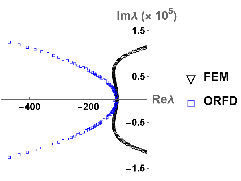
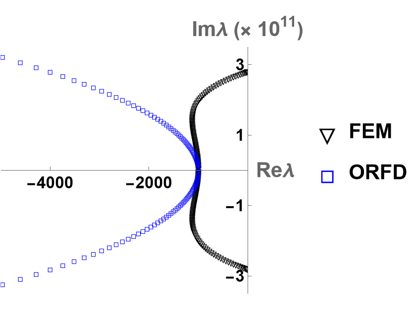
Figure 1: For $N=80$, the spectral graph for each branch of FEM and ORFD eigenvalues show that the ORFD model reduction is more robust for the model reduction of the PDE model without any type of numerical filtering.

Next, we set up the numerical filtering for the FEM model reduction (44). Since the high-frequency eigenvalues approach the imaginary axis, the numerical filtering ensures that the eigenvalues are bounded away from the imaginary axis. Let $\left\{\lambda^{\pm}_{1j},\lambda^{\pm}_{2j}\right\}(h)$ and $\left\{{\vec{\Psi}^{\pm 1}},{\vec{\Psi}^{\pm 2}}\right\}(h)$ be the eigenvalues and eigenvectors of (44). Recall that there exist two branches of eigenvalues associated with $v(x,t)$ and $p(x,t)$. We define direct Fourier filtering parameter $j^{*}$, i.e. see [13, 32], such that ${\mathcal{C}}_{h}(j^{*})$ represents the filtered solutions of (44) and it is defined as the following

$$\begin{array}[]{ll}{\mathcal{C}}_{h}(j^{*}):=\sum\limits_{j=1}^{N+1-j^{*}}\left[c_{1j}{\vec{\Psi}}^{+1}e^{\tilde{\lambda}^{+}_{1j}t}+d_{1j}{\vec{\Psi}^{-1}}e^{{\tilde{\lambda}}^{-}_{1j}t}\right.&\\ \left.\qquad\qquad\qquad+c_{2j}{\vec{\Psi}}^{+2}e^{\tilde{\lambda}^{+}_{2j}t}+d_{2j}{\vec{\Psi}^{-2}}e^{-{\tilde{\lambda}}^{-}_{2j}t}\right]\end{array}$$ (281)

where $j^{*}$ is number of the conjugate pair of the eigenvalues filtered from each branch. Noticing if $j^{*}\to 0$, there is little filtering, and if $j^{*}\to N,$ there is too much filtering.

Next, we consider three different choices of the number of nodes $N=40,~{}80,~{}160$. Observe in Table 2 that for the FEM case, without filtering, i.e. (i) $j^{*}=0$, the maximum real part of the eigenvalues approaches to $0$ as $N$ gets larger. This shows that the FEM solutions behave super badly. With some filtering, i.e. (ii) $j^{*}=5$ and (iii) $j^{*}=10,$ the maximum real parts of the eigenvalues diverge away from the imaginary axis. Moreover, slow exponential decay rates can be also observed. On the other hand, for the ORFD case, the maximum real parts of the eigenvalues for different choices of $N$ are already uniformly bounded away from the imaginary axis regardless of the choice of $N$. Unlike FEM solutions, ORFD solutions exponentially decay faster without any need of filtering for each choice of $N$.

Table 2: FEM vs. ORFD in terms of maximum real part of eigenvalues.

Method	Fourier Filtering	Maximum real part of eigenvalues
	$j^{*}$	N = 40	N = 80	N = 160
	0	-1.31141	-0.337577	-0.0855461
FEM	5	-38.4174	-11.4988	-3.03642
	10	-85.1029	-34.023	-9.865
ORFD	N/A	-101.967	-101.938	-101.759

Recalling from Section 2 that the FEM solutions behave badly for high-frequency vibrational modes. Therefore, for simulation purposes, all initial conditions are intentionally chosen as a high-frequency type. Letting $N=80$,

$$v_{0}(x_{j}),p_{0}(x_{j}),v_{1}(x_{j}),p_{1}(x_{j})=10^{-2}\sum\limits_{k=41}^{81}jh\sin(k\pi x_{j}).$$

The final time of the simulation is chosen as $T_{\rm final}=0.1$ sec. As seen in the first row in Figure 2, the high frequency vibrational modes of the FEM solutions do not decay at all. Hence, this results in an unrealistic approximation of the PDE model. After some filtering, the spurious high-frequency vibrational modes are eliminated, and a more realistic approximation of the PDE is obtained, i.e. see the second row in Figure 2. On the other hand, the ORFD solutions exponentially decay without any need of filtering, see Figure 3.

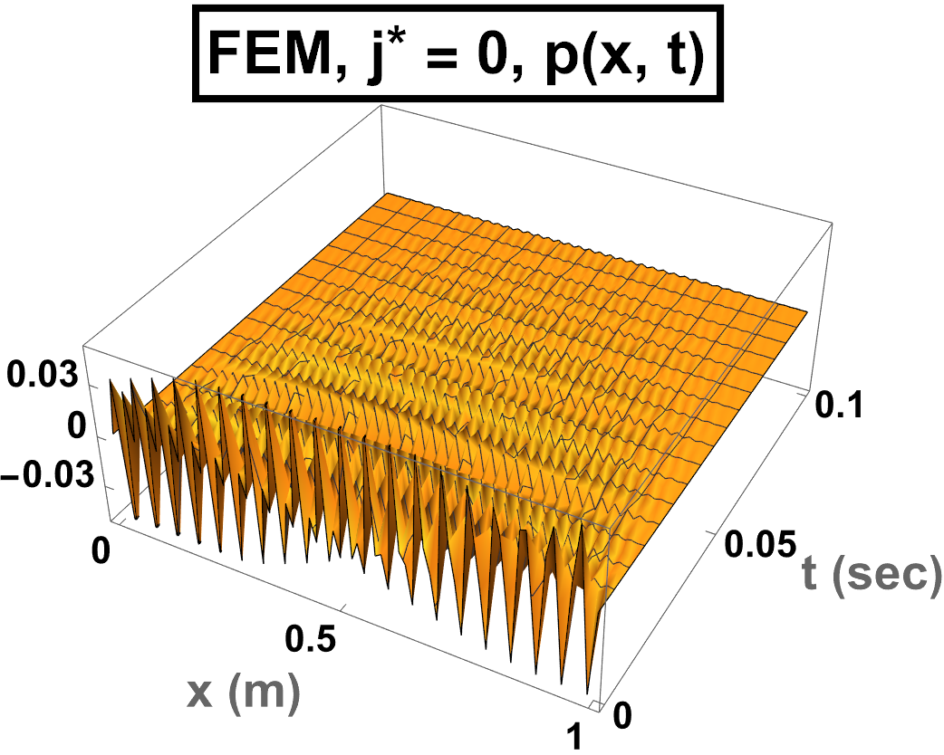
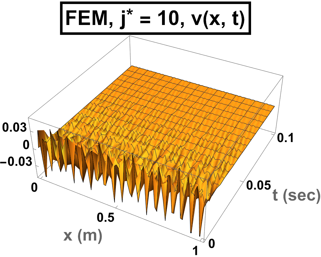
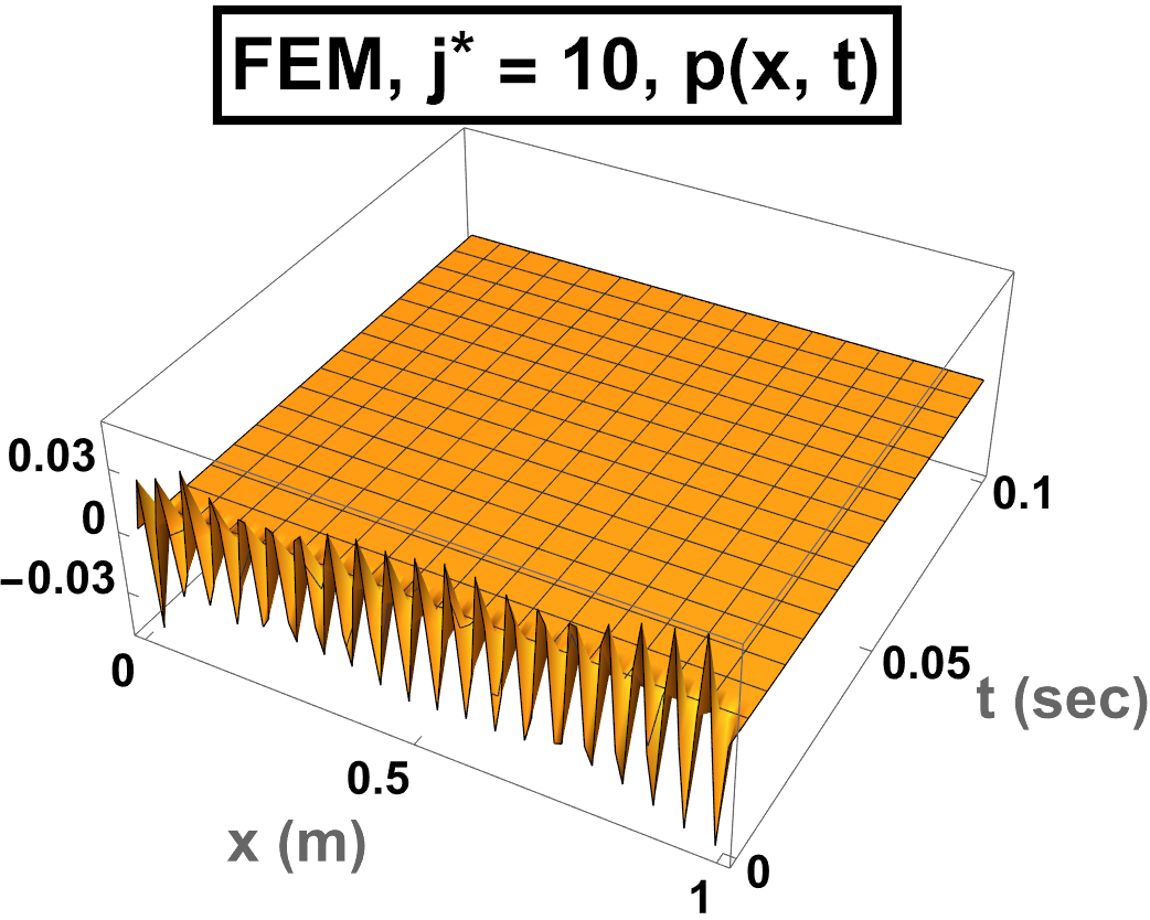
Figure 2: The first row shows $v(x,t)$ and $p(x,t)-$solutions by FEM without any filtering. The high-frequency modes especially for the $v$-solution do not decay. The second row shows the fast exponential decay once some of the high-frequency modes are filtered, i.e. $j^{*}=10$.

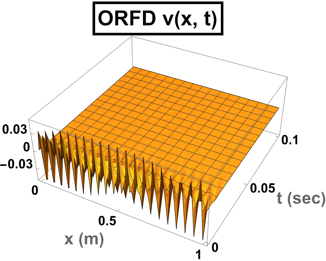
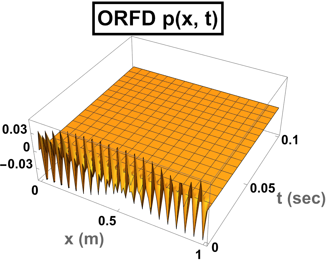
Figure 3: Without the need of any filtering, ORFD solutions decay fast enough, expectedly mimicking the PDE counterpart.

For the interested audience, real-time Wolfram demonstrations of the magnetizable piezoelectric dynamics can be reached at [44].

7 Conclusions & Future Work

In this paper, an FEM-based model reduction for the magnetizable piezoelectric beam with linear splines is proposed for the first time. Since this reduction does not preserve the exponential stability of the solutions of the PDE uniformly as the discretization parameter tends to zero especially if there is no proper Fourier filtering. Alternatively, an order-reduction based model reduction by Finite Differences is proposed for the first time for the considered PDE model. The exponential stability of the reduced model is established by a clever use of Lyapunov theory, and the convergence of the energy is also proved as the discretization parameter tends to zero. This method lays a foundation for robust model reductions of multi-layer systems involving piezoelectric layers [26]-[27], [29]-[33].

Ahmet Özkan Özer (Member, IEEE) received an M.Sc. degree in Mechanical Engineering from Istanbul Technical University (Turkiye) in 2004, another M.Sc. degree in Pure Mathematics from ICTP (Italy) in 2006, and a Ph.D. degree in Applied Mathematics from Iowa State University (USA) in 2011. He held two postdoctoral positions: one at the University of Waterloo (Canada) from 2011 to 2013, and another one at the University of Nevada-Reno (USA) from 2013 to 2016. He is currently an Associate Professor of Mathematics at Western Kentucky University (USA). As part of a sabbatical leave, Ahmet Özkan Özer is a visiting professor at both the Friedrich-Alexander-Universität Erlangen-Nürnberg in Germany and the Université Polytechnique Hauts-de-France in France in 2023. His research interests include modeling, controllability, and model reductions of smart material systems modeled by partial differential equations.

Ahmet Kaan Aydin (Member, IEEE) received a Bachelor’s degree in Mathematics from Yildiz Technical University (Turkiye) in 2020, and an M.Sc. degree in Mathematics from Western Kentucky University (USA) in 2022. Ahmet is currently pursuing a Ph.D. degree in Applied Mathematics at the University of Maryland, Baltimore County.

Jacob Walterman (Member, IEEE) is currently a senior at Western Kentucky University (USA). Jacob is double majoring in Mathematics and Computer Science.

References

[1]M. Afilal, A. Soufyane, M. de Lima Santos. Piezoelectric beams with magnetic effect and localized damping. Mathematical Control and Related Fields 13-1 (2023), 250-264.
[2] C. Baur, D.J. Apo, D. Maurya, S. Priya, M. Voit, Piezoelectric Polymer Composites for Vibrational Energy
Harvesting, American Chemical Society. Washington, DC, 2014.
[3] U. Biccari, A. Marica, E. Zuazua Propagation of One-and Two-Dimensional Discrete Waves Under Finite Difference Approximation,Found. Comput. Math., vol. 20, 2020, 1401–1438.
[4] H.T. Banks, A functional analysis framework for modeling, estimation and control in science and engineering, CRC Press, 2012.
[5] H.T. Banks, K. Ito, C. Wang, Exponentially stable approximations of
weakly damped wave equations, in: Estimation and Control of Distributed
Parameter Systems, Springer-Basel, 1991, 1–33.
[6] H.E. Boujaoui, H. Bouslous, L. Maniar, Boundary Stabilization for 1-d Semi-Discrete Wave Equation by Filtering Technique Bulletin of TICMI (17-1) 2013, 1–18.
[7] A.N. Darinskii, E. Le Clezio, G. Feuillard, The role of electromagnetic waves in the reflection of acoustic waves
in piezoelectric crystals, Wave Motion. 45 (2008), 428–444.
[8] M.C. de Jong, K.C. Krishna, J.M.A. Scherpen. On control of voltage-actuated piezoelectric beam: A Krasovskii passivity-based approach, European Journal of Control 69 (2023), 100724.
[9] B. Feng, A. Ö. Özer, Stability results for piezoelectric beams with long‐range memory effects in the boundary, Mathematische Nachrichten, 2023.
[10] B. Feng, A. Ö. Özer, Exponential stability results for the boundary-controlled fully-dynamic piezoelectric beams with various distributed and boundary delays, Journal of Mathematical Analysis and Applications, 508-1 (2022), 125845.
[11] M.M. Freitas, A. Ö. Özer, A.J.A. Ramos, Long time dynamics and upper semi-continuity of attractors for piezoelectric beams with nonlinear boundary feedback, ESAIM: Control, Optimisation and Calculus of Variations 28 (2022): 39.
[12] A. Guesmia, On the L 2 (R)-Norm Decay Estimates for Two Cauchy Systems of Coupled Wave Equations Under Frictional Dampings, Communications on Applied Mathematics and Computation, 1-20 (2023).
[13] J.A Infante and E. Zuazua, Boundary observability for the space semi-discretizations of the 1-D wave
equation,Math. Model. Num. Ann., vol. 33, 1999, pp. 407-438.
[14] V. Komornik, Exact Controllability and Stabilization. The Multiplier Method, RAM. Masson-John Wiley, Paris, 1994.
[15] L. Leon, E. Zuazua, Boundary controllability of the finite-difference space semi-discretizations of the beam equation, ESAIM Control Opt. Calc. Var., (8) 2002, 827-862.
[16]J. Liu, B.Z. Guo, A novel semi-discrete scheme preserving uniformly exponential stability for an Euler Bernoulli beam, Systems & Control Letters, (134) 2019, 104518.
[17] J. Liu, B.Z.Guo, A new semi-discretized order reduction finite difference scheme for uniform approximation of 1-d wave equation, SIAM Journal on Control and Optimization, (58) 2020, 2256-228.
[18] J. Liu, B.Z. Guo, Uniformly semi-discretized approximation for exact observability and controllability of one-dimensional Euler-Bernoulli beam, Systems & Control Letters (156) 2021, 105013.
[19] A. Kong, C. Nonato, W. Liu, M.J.D Santos, C. Raposo, Equivalence between exponential stabilization and observability inequality for magnetic effected piezoelectric beams with time-varying delay and time-dependent weights, Discrete & Continuous Dynamical Systems-Series B, 27-6 (2022).
[20] P. Lissy, I. Roventa, Optimal filtration for the approximation of boundary controls for the one-dimensional wave equation using finite-difference method, Math. Comp., 88, 273-291, 2019.
[21] K. Morris, A.Ö. Özer, Modeling and stability of voltage-actuated piezoelectric beams with electric effect, SIAM J. Control Optimum, (52-4), 2371-2398, 2014.
[22] A.Ö. Özer, Further stabilization and exact observability results for voltage-actuated piezoelectric beams with magnetic effects, Math. Control Signals Systems, 27 (2015), 219–244.
[23] A.Ö. Özer, R. Emran, Revisiting the Direct Fourier Filtering Technique for the Maximal Decay Rate of Boundary-damped Wave Equation by Finite Differences and Finite Elements, arXiv: 2306.11398, 2023.
[24] A.Ö. Özer, R. Emran, A.K. Aydin, Maximal Decay Rate and Optimal Sensor Feedback Amplifiers for Fast Stabilization of Magnetizable Piezoelectric Beam Equations, arXiv: 2306.10705, 2023.
[25] A.Ö. Özer, R. Emran, A.K. Aydin, A Robust Model Reduction for the Boundary Feedback Stabilization of Piezoelectric Beams, submitted, 2023.
[26] A.Ö. Özer, M. Khenner, An alternate numerical treatment for nonlinear PDE models of piezoelectric laminates, Proc. SPIE 10967, Active and Passive Smart Structures and Integrated Systems XII, 109671R, 2019.
[27] A.Ö. Özer, Modeling and controlling an active constrained layered (ACL) beam actuated by two voltage sources with/without magnetic effects, IEEE Trans. Automat. Contr., (62-12), 6445–6450, 2017.
[28] A.Ö. Özer, Potential formulation for charge or current-controlled piezoelectric smart composites and stabilization results: electrostatic vs. quasi-static vs. fully-dynamic approaches, IEEE Trans. Automat. Contr., (64-3), 989-1002, 2019.
[29] A.Ö. Özer, Uniform boundary observability of semi-discrete finite difference approximations of a Rayleigh beam equation with only one boundary observation, IEEE Conference on Decision and Control (CDC), Nice, France, 2019, 7708–7713.
[30] A.Ö. Özer, Stabilization results for well-posed potential formulations of a current-controlled piezoelectric beam and their approximations. Applied Mathematics & Optimization 84-1 (2021), 877-914.
[31] A.Ö. Özer, A.K. Aydin, Uniform boundary observability of filtered finite difference approximations of a Mead-Marcus sandwich beam equation with only one boundary observation, IEEE Conference on Decision and Control, Cancun, Mexico, 2022, 6535-6541.
[32] A.Ö. Özer, W. Horner, Uniform boundary observability of Finite Difference approximations of non-compactly-coupled piezoelectric beam equations, Applicable Analysis, (101-5), 1571-1592.
[33] A.Ö. Özer, A.K. Aydin, J. Walterman, A Novel Finite Difference-based Model Reduction and a Sensor Design for a Multilayer Smart Beam with Arbitrary Number of Layers, IEEE Control Systems Letters, 7 (2023), 1548-1553.
[34] G.H. Peichl, C. Wang, Asymptotic analysis of stabilizability of a control system for a discretized boundary damped wave equation, Numerical Functional Analysis and Optimization, (19:1-2) 1998, 91-113.
[35] A. Preumont, Vibration control of active structures: an introduction 246 (2008). Springer.
[36] V. Poblete, F. Toledo, O, Vera. Polynomial stability of a piezoelectric beam with magnetic effect and a boundary dissipation of the fractional derivative type, Proceedings of the Edinburgh Mathematical Society, (2023): 1-31.
[37] A.J.A. Ramos, J.A. C.S. Goncalves, S.S.C. Neto. Exponential stability and numerical treatment for piezoelectric beams with magnetic effect, ESAIM: Mathematical Modeling and Numerical Analysis, 52.1 (2018), 255-274.
[38] A.J.A. Ramos, M. M. Freitas, D. S. Almeida Jr., S.S. Jesus, T.R.S. Moura, Equivalence between exponential stabilization and boundary observability for piezoelectric beams with magnetic effect, Zeitschrift für angewante Mathematik und Physik (ZAMP,) 70-60 (2019).
[39] A.J.A. Ramos, A. Ö Özer, M.M. Freitas, D.S. Almeida Júnior, J.D. Martins. Exponential stabilization of fully dynamic and electrostatic piezoelectric beams with delayed distributed damping feedback, Zeitschrift für angewandte Mathematik und Physik 72 (2021), 1-15.
[40] R.C. Smith, Smart Material Systems, Society for Industrial and Applied Mathematics, Philadelphia, PA, 2005.
[41] D. Tallarico, N. Movchan, A. Movchan, M. Camposaragna, M, Propagation and filtering of elastic and electromagnetic waves in piezoelectric composite structures Math. Meth. Appl. Sc. 40 (2017), 3202–3220.
[42] L.T. Tebou, E. Zuazua. Uniform boundary stabilization of the finite difference space discretization of the 1-d wave equation. Adv. Comput. Math., 26, 337-365, 2007.
[43] T. Voss, J.M.A. Scherpen, Stabilization and shape control of a 1D piezoelectric Timoshenko beam, Automatica, (47-12),
2780-85, 2011.
[44]J. Walterman, A.K. Aydin, S. Leveridge, A. Ö Özer, Dynamics of a Longitudinal Piezoelectric Beam, Wolfram Demonstrations Project, Published: June 2023, http://demonstrations.wolfram.com/DynamicsOfALongitudinalPiezoelectricBeam/.
[45] J. Yang, Fully-dynamic Theory. In: Yang J. (eds) Special Topics in the Theory of Piezoelectricity. Springer. New York, 2009.
[46] H-E. Zhang, X. G-Q Xu, Z-J Han, Stability and Eigenvalue Asymptotics of Multi-Dimensional Fully Magnetic Effected Piezoelectric System with Friction-Type Infinite Memory, SIAM Journal on Applied Mathematics 83-2 (2023), 510-529.
[47] E. Zuazua, Controllability of Partial Differential Equations, 2006.
{IEEEbiographynophoto}