[ansaetze]ansätze spacing=nonfrench

Precision calculation of the electromagnetic radii of the proton and neutron
from lattice QCD

Abstract

We present lattice-QCD results for the electromagnetic form factors of the proton and neutron including both quark-connected and -disconnected contributions. The parametrization of the $Q^{2}$-dependence of the form factors is combined with the extrapolation to the physical point. In this way, we determine the electric and magnetic radii and the magnetic moments of the proton and neutron. For the proton, we obtain at the physical pion mass and in the continuum and infinite-volume limit $\sqrt{\langle r_{E}^{2}\rangle^{p}}=\qty{0.820(14)}{fm}$, $\sqrt{\langle r_{M}^{2}\rangle^{p}}=\qty{0.8111(89)}{fm}$, and $\mu_{M}^{p}=$2.739(66)$$, where the errors include all systematics.

Introduction.

The so-called “proton radius puzzle”, the observation of a large tension in the proton’s electric (charge) radius extracted either from atomic spectroscopy data of muonic hydrogen [1, 2] or, alternatively, from corresponding measurements on electronic hydrogen [3] as well as $ep$-scattering data [4, 5], has gripped the scientific community for more than 10 years and triggered a vigorous research effort designed to explain the discrepancy.

Recent results determined from $ep$-scattering data collected by the PRad experiment [6] and from atomic hydrogen spectroscopy [7, 8, 9] (with the exception of Ref. [10]) point towards a smaller electric radius, as favored by muonic hydrogen and dispersive analyses of $ep$-scattering data [11, 12, 13, 14]. To allow for a more reliable and precise determination of the proton’s electromagnetic form factors from which the radii are extracted, efforts are underway to extend $ep$-scattering experiments to unprecedentedly small momentum transfers [15, 16, 17], which are complemented by plans to perform high-precision measurements of $\mu p$ cross sections [18, 19].

While the situation regarding the electric radius is awaiting its final resolution, one also finds discrepant results for the proton’s magnetic radius. Specifically, there is a tension of $2.7\,\sigma$ between the value extracted from the A1 $ep$-scattering data alone and the estimate from the corresponding analysis applied to the remaining world data [20]. Clearly, a firm theoretical prediction for basic properties of the proton and the neutron, such as their radii and magnetic moments, would be highly desirable in order to assess our understanding of the particles that make up the largest fraction of the visible mass in the universe.

In this letter we present our results for the radii and magnetic moment of the proton computed in lattice QCD. Compared with previous lattice studies [21, 22, 23, 24, 25, 26, 27, 28, 29, 30, 31, 32, 33, 34, 35, 36, 37, 38], our calculation is the first to include the contributions from quark-disconnected diagrams while controlling all sources of systematic uncertainties arising from excited-state contributions, finite-volume effects and the continuum extrapolation. We determine the proton’s magnetic radius $\sqrt{\langle r_{M}^{2}\rangle^{p}}$ with a total precision of 1.1, which is competitive with recent analyses of $ep$-scattering data [4, 20, 12, 13]. Moreover, our lattice QCD estimate for the proton’s magnetic moment is in good agreement with experiment. Our result for the electric radius, which has a total precision of 1.7, is consistent with the value determined in muonic hydrogen within 1.5 standard deviations.

Lattice setup.

Our aim is to compute the electric and magnetic Sachs form factors $G_{E}(Q^{2})$ and $G_{M}(Q^{2})$ of the proton and neutron. The electric form factor at zero momentum transfer yields the nucleon’s electric charge, $G_{E}^{p}(0)=1$ and $G_{E}^{n}(0)=0$, whereas the magnetic form factor at $Q^{2}=0$ is identified with the magnetic moment, $G_{M}(0)=\mu_{M}$. The radii can in turn be extracted from the slope of the form factors at zero momentum transfer,

$$\langle r^{2}\rangle=-\frac{6}{G(0)}\left.\frac{\partial G(Q^{2})}{\partial Q^{2}}\right|_{Q^{2}=0}.$$ (1)

The only exception to this definition is the electric radius of the neutron, where the normalization factor $1/G(0)$ is dropped.

For our lattice determination of these quantities, we use the ensembles generated by the Coordinated Lattice Simulations (CLS) [39] effort with $2+1$ flavors of non-perturbatively $\mathcal{O}(a)$-improved Wilson fermions [40, 41] and a tree-level improved Lüscher-Weisz gauge action [42], correcting for the treatment of the strange quark determinant using the procedure outlined in Ref. [43]. Table 1 shows the set of ensembles entering the analysis: they cover four lattice spacings in the range from 0.050fm to 0.086fm, and several pion masses, including one slightly below the physical value (E250). Further details on our setup of the simulations and the measurements of the two- and three-point functions of the nucleon can be found in the accompanying paper [44].

Table 1: Overview of the ensembles used in this study. Further details are contained in table I of the accompanying paper [44].

ID	$\beta$	$t_{0}^{\mathrm{sym}}/a^{2}$	$T/a$	$L/a$	$M_{\pi}$ [MeV]
C101	3.40	2.860(11)	96	48	227
N101	3.40	2.860(11)	128	48	283
H105	3.40	2.860(11)	96	32	283
D450	3.46	3.659(16)	128	64	218
N451	3.46	3.659(16)	128	48	289
E250	3.55	5.164(18)	192	96	130
D200	3.55	5.164(18)	128	64	207
N200	3.55	5.164(18)	128	48	281
S201	3.55	5.164(18)	128	32	295
E300	3.70	8.595(29)	192	96	176
J303	3.70	8.595(29)	192	64	266

To extract the effective form factors from two- and three-point correlation functions, we employ the ratio method [45] and the same estimators for the effective electric and magnetic Sachs form factors as in Ref. [37]. For further technical details, we again refer to the companion paper [44]. The effective form factors are constructed for the isovector ($u-d$) and the connected isoscalar ($u+d$) combinations, as well as for the light and strange disconnected contributions. In the isovector case, the disconnected contributions cancel. The full isoscalar (octet) combination $u+d-2s$, on the other hand, is obtained from the connected and disconnected pieces as

$$G_{E,M}^{\mathrm{eff},u+d-2s}=G_{E,M}^{\mathrm{eff,conn},u+d}+2G_{E,M}^{\mathrm{eff,disc},l-s}.$$ (2)

Note that the disconnected part only requires the difference $l-s$ between the light and strange contributions, in which correlated noise cancels and which can be computed efficiently by the one-end trick [46, 47, 48].

We express all dimensionful quantities in units of the gradient flow time $t_{0}$ [49] using the determination of $t_{0}^{\mathrm{sym}}/a^{2}$ from Ref. [50]. Only in the final step, after the extrapolation to the physical point, are the radii converted to physical units by means of the FLAG estimate of

$$\sqrt{t_{0,\mathrm{phys}}}=\qty{0.14464(87)}{fm}$$ (3)

for $N_{f}=2+1$ from Ref. [51].

Excited-state analysis.

Due to the strong exponential decay of the signal-to-noise ratio for baryonic correlation functions with increasing source-sink separation [52, 53], an explicit treatment of the excited-state systematics is required in order to extract the ground-state form factors from the effective ones [54]. In this work, we employ the summation method [55, 56, 57]. It exploits the fact that the contributions from excited states to effective form factors are parametrically more strongly suppressed when the insertion of the electromagnetic current is summed over timeslices between the source and sink. In the asymptotic limit, the slope of the summed correlator ratio with respect to the source-sink separation $t_{\mathrm{sep}}$ yields the ground-state form factor [30, 37].

In our analysis, we monitor the stability of fit results for different starting values $t_{\mathrm{sep}}^{\mathrm{min}}$ of the source-sink separation. Rather than selecting one particular value of $t_{\mathrm{sep}}^{\mathrm{min}}$ on each ensemble, we perform a weighted average over $t_{\mathrm{sep}}^{\mathrm{min}}$, where the weights are given by a smooth window function [58, 59] [cfeq. (18) in the accompanying paper [44]].

This averaging strategy is illustrated in fig. 1 for the isoscalar combination at the first non-vanishing momentum on ensemble E300. One finds that the window averages agree within their errors with what one can identify as plateaux in the blue points. This is observed for practically all other ensembles and momenta employed in the analysis, and hence we conclude that the window method reliably isolates the asymptotic value. Moreover, it reduces the human bias arising from manually picking one particular value for $t_{\mathrm{sep}}^{\mathrm{min}}$ on each ensemble, because we use the same window parameters in units of $t_{0}$ on all ensembles. Since our window average does not yield a significantly smaller error in comparison with the individual points entering the average (cffig. 1), we are confident that our error estimates are sufficiently conservative to exclude any systematic bias in estimating the ground-state form factors.

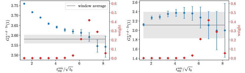
Figure 1: Isoscalar electromagnetic form factors at the lowest non-vanishing momentum ($Q^{2}\approx\qty{0.067}{GeV^{2}}$) on ensemble E300 as a function of the minimal source-sink separation entering the summation fit. Each blue point corresponds to a single fit starting at the value given on the horizontal axis. The associated weights in the average are represented by the red diamonds, with the gray curves and bands depicting the averaged results.

Direct B$\chi$PT fits.

To extract the radii from the form factors, we need to describe the $Q^{2}$-dependence of the latter. As in Refs. [30, 37], we employ two different methods: our preferred procedure is to combine the parametrization of the $Q^{2}$-dependence with the extrapolation to the physical point ($M_{\pi}=M_{\pi,\mathrm{phys}}$, $a=0$, $L=\infty$) by fitting our form factor data directly to the expressions resulting from covariant baryon chiral perturbation theory (B$\chi$PT) [60]. This is presented in the following. Alternatively, we have implemented the more traditional strategy of first performing a generic parametrization of the $Q^{2}$-dependence on each ensemble, followed by extrapolating the resulting radii to the physical point. A crosscheck of our main analysis with this two-step approach can be found in the accompanying paper [44].

For our main analysis, we fit our form factor data to the full expressions of Ref. [60] without explicit $\Delta$ degrees of freedom. The fits are performed for the isovector and isoscalar channels separately, but for $G_{E}$ and $G_{M}$ simultaneously. This allows us to properly treat the correlations between different $Q^{2}$ and also between $G_{E}$ and $G_{M}$. Different gauge ensembles, on the other hand, are treated as statistically independent. In the isovector channel, we include the contributions from the $\rho$ meson in the expressions for the form factors, while in the isoscalar channel, we include the leading-order terms from the $\omega$ and $\phi$ resonances. The physical pion mass $M_{\pi,\mathrm{phys}}$ is fixed in units of $\sqrt{t_{0}}$ using its value in the isospin limit [61],

$$M_{\pi,\mathrm{phys}}=M_{\pi,\mathrm{iso}}=\qty{134.8(3)}{MeV},$$ (4)

we employ $\sqrt{t_{0,\mathrm{phys}}}M_{\pi,\mathrm{phys}}=0.09881(59)$. Here, we neglect the uncertainty of $M_{\pi,\mathrm{iso}}$ in MeV since it is completely subdominant compared to that of $\sqrt{t_{0,\mathrm{phys}}}$ which enters in the conversion of units. We perform several such fits with various cuts in the pion mass ($M_{\pi}\leq\qty{0.23}{GeV}$ and $M_{\pi}\leq\qty{0.27}{GeV}$) and the momentum transfer ($Q^{2}\leq\qtyrange[range-phrase={,\ldots,},range-units=single]{0.3}{0.6}{GeV^{2}}$), as well as with different models for the lattice-spacing and/or finite-volume dependence, in order to estimate the corresponding systematic uncertainties. We reconstruct the proton and neutron form factors as linear combinations of the B$\chi$PT formulae for the isovector and isoscalar channels, evaluating the low-energy constants as determined from the separate fits in these channels. For further technical details of the fits, we refer to the accompanying paper [44].

The major benefits of the direct approach compared to the two-step procedure have been previously observed in our publication on the isovector electromagnetic form factors [37]: Firstly, including multiple ensembles in one fit significantly reduces the resulting errors on the radii. Secondly, it greatly increases the number of degrees of freedom in the fit, which has a stabilizing effect with regard to lowering the momentum cut.

Model average and final results.

Since we do not have a strong preference for one specific setup of the direct fits, we determine our final results and total errors from averages over different fit models and kinematic cuts. For this purpose, we use weights derived from the Akaike Information Criterion [62, 63, 64, 65, 66]. In order to estimate the statistical and systematic uncertainties of our model averages, we adopt a bootstrapped variant of the method from Ref. [67]. Our procedure is explained in more detail in the accompanying paper [44]. As our final results, we obtain

$$\langle r_{E}^{2}\rangle^{p} =\qty{0.672(14)(18)}{fm^{2}},$$ (5)

$$\langle r_{M}^{2}\rangle^{p} =\qty{0.658(12)(8)}{fm^{2}},$$ (6)

$$\mu_{M}^{p} =$2.739(63)(18)$,$$ (7)

$$\langle r_{E}^{2}\rangle^{n} =\qty{-0.115(13)(7)}{fm^{2}},$$ (8)

$$\langle r_{M}^{2}\rangle^{n} =\qty{0.667(11)(16)}{fm^{2}},$$ (9)

$$\mu_{M}^{n} =$-1.893(39)(58)$.$$ (10)

We note that the precision of the magnetic radius of the proton, $\sqrt{\langle r_{M}^{2}\rangle^{p}}=\qty{0.8111(74)(50)}{fm}$, is commensurate with that of its electric counterpart, $\sqrt{\langle r_{E}^{2}\rangle^{p}}=\qty{0.820(9)(11)}{fm}$.

Figure 2: Electromagnetic form factors of the proton as a function of $Q^{2}$. The orange curves and bands correspond to our final results at the physical point with their full uncertainties obtained as model averages over the different direct fits. The light orange bands indicate the statistical errors. The black diamonds represent the experimental $ep$-scattering data by the A1 Collaboration [4] obtained using Rosenbluth separation. The experimental value of the magnetic moment [68] is depicted by a red cross.

To further compare our results to experiment we perform model averages of the form factors themselves. The results are plotted in fig. 2 for the proton. One observes that the slope of the electric form factor differs slightly between our calculation and the measurement by the A1 Collaboration [4] over the whole range of $Q^{2}$. The magnetic form factor, on the other hand, agrees well with the A1 data. Moreover, our estimates reproduce within their errors the experimental results for the magnetic moments both of the proton and of the neutron [68]. The plots for the neutron corresponding to fig. 2 in this letter are contained in fig. 7 of the accompanying paper [44].

In fig. 3, our results for the electromagnetic radii and magnetic moment of the proton are compared to recent lattice determinations and to the experimental values. We note that the only other lattice result including disconnected contributions is ETMC19 [35], which, however, has not been extrapolated to the continuum and infinite-volume limits. Our estimate for the electric radius is larger than the results of Refs. [35, 36, 34], while Ref. [28] quotes an even larger central value.

We stress that any difference between our estimate and previous lattice calculations is not related to our preference for direct fits to the form factors over the conventional approach via the $z$-expansion, as the latter yields similar values for $\sqrt{\langle r_{E}^{2}\rangle^{p}}$ for our data (cfthe accompanying paper [44]). For the magnetic radius, our result agrees with that of Refs. [35, 34] within $1.2$ combined standard deviations, while that of Ref. [27] is much smaller. Our statistical and systematic error estimates for the electric radius and magnetic moment are similar or smaller compared to other lattice studies, while being substantially smaller for the magnetic radius. As a final remark we note that the lack of a data point at $Q^{2}=0$ complicates the extraction of the magnetic low-$Q^{2}$ observables in most recent lattice determinations, especially for $z$-expansion fits on individual ensembles. By contrast, the direct approach – in addition to combining information from several ensembles and from $G_{E}$ and $G_{M}$ – is more constraining at low $Q^{2}$, allowing for considerably less variation in the form factors in that regime. We believe this to be responsible, to a large extent, for the small errors we achieve in the magnetic radii.

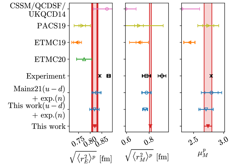
Figure 3: Comparison of our best estimates for the electromagnetic radii and the magnetic moment of the proton with other lattice calculations, Mainz21 [37], ETMC20 [36], ETMC19 [35], PACS19 [34], and CSSM/QCDSF/UKQCD14 [27, 28]. Only ETMC19 and this work include disconnected contributions. The Mainz21 values have been obtained by combining their isovector results with the PDG values for the neutron [68]. We also show this estimate using our updated isovector results (cfthe accompanying paper [44]). The experimental value for $\mu_{M}^{p}$ is taken from PDG [68]. The two data points for $\sqrt{\langle r_{E}^{2}\rangle^{p}}$ depict the values from PDG [68] (cross) and Mainz/A1 [4] (square), respectively. The two data points for $\sqrt{\langle r_{M}^{2}\rangle^{p}}$, on the other hand, show the reanalysis of Ref. [20] either using the world data excluding that of Ref. [4] (diamond) or using only that of Ref. [4] (square).

Conclusions.

We have performed the first lattice QCD calculation of the radii and magnetic moment of the proton to include the contributions from quark-connected and -disconnected diagrams and present a full error budget. The overall precision of our calculation is sufficient to make a meaningful contribution to the debate surrounding the proton radii. Our final estimates are listed in eqs. 5, 6, 7, 8, 9 and 10.

As an important benchmark, we reproduce the experimentally very precisely known magnetic moments of the proton and neutron [68] within our quoted uncertainties. A detailed discussion of our results for the neutron radii can be found in the accompanying paper [44]. Our result for the electric (charge) radius of the proton is much closer to the value inferred from muonic hydrogen spectroscopy [2] and the recent $ep$-scattering experiment by PRad [6] than to the A1 $ep$-scattering result [4]. For the magnetic radius, on the other hand, our estimate is well compatible with the analyses [4, 20] of the A1 data and exhibits a $2.8\,\sigma$ tension with the other collected world data [20]. The analyses of combined A1+PRad data [13] and A1 data alone [12], based respectively on dispersive and dispersively improved fit , arrive at values of $\sqrt{\langle r_{M}^{2}\rangle^{p}}$ that are significantly larger than the A1-data analysis [20] and in tension with our result. This could partly be due to unaccounted-for isospin-breaking effects. The shape of the magnetic form factor determined in our lattice calculation, however, agrees very well with the measurement by A1 [4] over the whole range of $Q^{2}$ under study.

Returning to the (electric) proton radius puzzle, our lattice results lend further support to the emerging consensus that the issue has essentially been settled [69, 70, 71]. Meanwhile, the situation regarding the magnetic radius remains to be clarified.

References

- Pohl et al. [2010] R. Pohl et al., The size of the proton, Nature 466, 213 (2010).
- Antognini et al. [2013] A. Antognini et al., Proton structure from the measurement of 2S-2P transition frequencies of muonic hydrogen, Science 339, 417 (2013).
- Mohr et al. [2012] P. J. Mohr, B. N. Taylor, and D. B. Newell, CODATA recommended values of the fundamental physical constants: 2010, Rev. Modern Phys. 84, 1527 (2012), arXiv:1203.5425 [physics.atom-ph] .
- Bernauer et al. [2014] J. C. Bernauer et al. (A1 Collaboration), Electric and magnetic form factors of the proton, Phys. Rev. C 90, 015206 (2014), arXiv:1307.6227 [nucl-ex] .
- Mihovilovič et al. [2021] M. Mihovilovič et al., The proton charge radius extracted from the initial-state radiation experiment at MAMI, Eur. Phys. J. A 57, 107 (2021), arXiv:1905.11182 [nucl-ex] .
- Xiong et al. [2019] W. Xiong et al., A small proton charge radius from an electron-proton scattering experiment, Nature 575, 147 (2019).
- Beyer et al. [2017] A. Beyer et al., The Rydberg constant and proton size from atomic hydrogen, Science 358, 79 (2017).
- Bezginov et al. [2019] N. Bezginov, T. Valdez, M. Horbatsch, A. Marsman, A. C. Vutha, and E. A. Hessels, A measurement of the atomic hydrogen Lamb shift and the proton charge radius, Science 365, 1007 (2019).
- Grinin et al. [2020] A. Grinin, A. Matveev, D. C. Yost, L. Maisenbacher, V. Wirthl, R. Pohl, T. W. Hänsch, and T. Udem, Two-photon frequency comb spectroscopy of atomic hydrogen, Science 370, 1061 (2020).
- Fleurbaey et al. [2018] H. Fleurbaey, S. Galtier, S. Thomas, M. Bonnaud, L. Julien, F. Biraben, F. Nez, M. Abgrall, and J. Guéna, New measurement of the transition frequency of hydrogen: Contribution to the proton charge radius puzzle, Phys. Rev. Lett. 120, 183001 (2018), arXiv:1801.08816 [physics.atom-ph] .
- Belushkin et al. [2007] M. A. Belushkin, H.-W. Hammer, and U.-G. Meißner, Dispersion analysis of the nucleon form factors including meson continua, Phys. Rev. C 75, 035202 (2007), arXiv:hep-ph/0608337 .
- Alarcón et al. [2020] J. M. Alarcón, D. W. Higinbotham, and C. Weiss, Precise determination of the proton magnetic radius from electron scattering data, Phys. Rev. C 102, 035203 (2020), arXiv:2002.05167 [hep-ph] .
- Lin et al. [2021] Y.-H. Lin, H.-W. Hammer, and U.-G. Meißner, High-precision determination of the electric and magnetic radius of the proton, Phys. Lett. B 816, 136254 (2021), arXiv:2102.11642 [hep-ph] .
- Lin et al. [2022] Y.-H. Lin, H.-W. Hammer, and U.-G. Meißner, New insights into the nucleon’s electromagnetic structure, Phys. Rev. Lett. 128, 052002 (2022), arXiv:2109.12961 [hep-ph] .
- Grieser et al. [2018] S. Grieser, D. Bonaventura, P. Brand, C. Hargens, B. Hetz, L. Leßmann, C. Westphälinger, and A. Khoukaz, A cryogenic supersonic jet target for electron scattering experiments at MAGIX@MESA and MAMI, Nucl. Instrum. Methods Phys. Res., Sect. A 906, 120 (2018), arXiv:1806.05409 [physics.ins-det] .
- Gasparian et al. [2022] A. Gasparian et al. (PRad Collaboration), PRad-II: A new upgraded high precision measurement of the proton charge radius, arXiv:2009.10510 [nucl-ex] (2022).
- Suda [2022] T. Suda, Low-energy electron scattering facilities in Japan, J. Phys.: Conf. Ser. 2391, 012004 (2022).
- Cline et al. [2021] E. Cline, J. Bernauer, E. J. Downie, and R. Gilman, MUSE: The MUon Scattering Experiment, SciPost Phys. Proc. 5, 023 (2021).
- Quintans [2022] C. Quintans (AMBER collaboration), The New AMBER Experiment at the CERN SPS, Few-Body Syst. 63, 72 (2022).
- Lee et al. [2015] G. Lee, J. R. Arrington, and R. J. Hill, Extraction of the proton radius from electron-proton scattering data, Phys. Rev. D 92, 013013 (2015), arXiv:1505.01489 [hep-ph] .
- Göckeler et al. [2005] M. Göckeler, T. R. Hemmert, R. Horsley, D. Pleiter, P. E. L. Rakow, A. Schäfer, and G. Schierholz (QCDSF Collaboration), Nucleon electromagnetic form factors on the lattice and in chiral effective field theory, Phys. Rev. D 71, 034508 (2005), arXiv:hep-lat/0303019 .
- Yamazaki et al. [2009] T. Yamazaki, Y. Aoki, T. Blum, H.-W. Lin, S. Ohta, S. Sasaki, R. Tweedie, and J. Zanotti (RBC and UKQCD Collaborations), Nucleon form factors with flavor dynamical domain-wall fermions, Phys. Rev. D 79, 114505 (2009), arXiv:0904.2039 [hep-lat] .
- Syritsyn et al. [2010] S. N. Syritsyn et al. (LHPC Collaboration), Nucleon electromagnetic form factors from lattice QCD using flavor domain wall fermions on fine lattices and chiral perturbation theory, Phys. Rev. D 81, 034507 (2010), arXiv:0907.4194 [hep-lat] .
- Bratt et al. [2010] J. D. Bratt et al. (LHPC), Nucleon structure from mixed action calculations using flavors of asqtad sea and domain wall valence fermions, Phys. Rev. D 82, 094502 (2010), arXiv:1001.3620 [hep-lat] .
- Alexandrou et al. [2013] C. Alexandrou, M. Constantinou, S. Dinter, V. Drach, K. Jansen, C. Kallidonis, and G. Koutsou, Nucleon form factors and moments of generalized parton distributions using twisted mass fermions, Phys. Rev. D 88, 014509 (2013), arXiv:1303.5979 [hep-lat] .
- Bhattacharya et al. [2014] T. Bhattacharya, S. D. Cohen, R. Gupta, A. Joseph, H.-W. Lin, and B. Yoon, Nucleon charges and electromagnetic form factors from -flavor lattice QCD, Phys. Rev. D 89, 094502 (2014), arXiv:1306.5435 [hep-lat] .
- Shanahan et al. [2014a] P. E. Shanahan, R. Horsley, Y. Nakamura, D. Pleiter, P. E. L. Rakow, G. Schierholz, H. Stüben, A. W. Thomas, R. D. Young, and J. M. Zanotti (CSSM and QCDSF/UKQCD Collaborations), Magnetic form factors of the octet baryons from lattice QCD and chiral extrapolation, Phys. Rev. D 89, 074511 (2014a), arXiv:1401.5862 [hep-lat] .
- Shanahan et al. [2014b] P. E. Shanahan, R. Horsley, Y. Nakamura, D. Pleiter, P. E. L. Rakow, G. Schierholz, H. Stüben, A. W. Thomas, R. D. Young, and J. M. Zanotti (CSSM and QCDSF/UKQCD Collaborations), Electric form factors of the octet baryons from lattice QCD and chiral extrapolation, Phys. Rev. D 90, 034502 (2014b), arXiv:1403.1965 [hep-lat] .
- Green et al. [2014] J. R. Green, J. W. Negele, A. V. Pochinsky, S. N. Syritsyn, M. Engelhardt, and S. Krieg, Nucleon electromagnetic form factors from lattice QCD using a nearly physical pion mass, Phys. Rev. D 90, 074507 (2014), arXiv:1404.4029 [hep-lat] .
- Capitani et al. [2015] S. Capitani, M. Della Morte, D. Djukanovic, G. von Hippel, J. Hua, B. Jäger, B. Knippschild, H. B. Meyer, T. D. Rae, and H. Wittig, Nucleon electromagnetic form factors in two-flavor QCD, Phys. Rev. D 92, 054511 (2015), arXiv:1504.04628 [hep-lat] .
- Alexandrou et al. [2017] C. Alexandrou, M. Constantinou, K. Hadjiyiannakou, K. Jansen, C. Kallidonis, G. Koutsou, and A. Vaquero Aviles-Casco, Nucleon electromagnetic form factors using lattice simulations at the physical point, Phys. Rev. D 96, 034503 (2017), arXiv:1706.00469 [hep-lat] .
- Hasan et al. [2018] N. Hasan, J. Green, S. Meinel, M. Engelhardt, S. Krieg, J. Negele, A. Pochinsky, and S. Syritsyn, Computing the nucleon charge and axial radii directly at in lattice QCD, Phys. Rev. D 97, 034504 (2018), arXiv:1711.11385 [hep-lat] .
- Ishikawa et al. [2018] K.-I. Ishikawa, Y. Kuramashi, S. Sasaki, N. Tsukamoto, A. Ukawa, and T. Yamazaki (PACS Collaboration), Nucleon form factors on a large volume lattice near the physical point in flavor QCD, Phys. Rev. D 98, 074510 (2018), arXiv:1807.03974 [hep-lat] .
- Shintani et al. [2019] E. Shintani, K.-I. Ishikawa, Y. Kuramashi, S. Sasaki, and T. Yamazaki (PACS Collaboration), Nucleon form factors and root-mean-square radii on a lattice at the physical point, Phys. Rev. D 99, 014510 (2019), erratum ibid. [76], arXiv:1811.07292 [hep-lat] .
- Alexandrou et al. [2019] C. Alexandrou, S. Bacchio, M. Constantinou, J. Finkenrath, K. Hadjiyiannakou, K. Jansen, G. Koutsou, and A. V. Aviles-Casco, Proton and neutron electromagnetic form factors from lattice QCD, Phys. Rev. D 100, 014509 (2019), arXiv:1812.10311 [hep-lat] .
- Alexandrou et al. [2020] C. Alexandrou, K. Hadjiyiannakou, G. Koutsou, K. Ottnad, and M. Petschlies, Model-independent determination of the nucleon charge radius from lattice QCD, Phys. Rev. D 101, 114504 (2020), arXiv:2002.06984 [hep-lat] .
- Djukanovic et al. [2021] D. Djukanovic, T. Harris, G. von Hippel, P. M. Junnarkar, H. B. Meyer, D. Mohler, K. Ottnad, T. Schulz, J. Wilhelm, and H. Wittig, Isovector electromagnetic form factors of the nucleon from lattice QCD and the proton radius puzzle, Phys. Rev. D 103, 094522 (2021), arXiv:2102.07460 [hep-lat] .
- Ishikawa et al. [2021] K.-I. Ishikawa, Y. Kuramashi, S. Sasaki, E. Shintani, and T. Yamazaki (PACS Collaboration), Calculation of derivative of nucleon form factors in lattice QCD at MeV on a (5.5 fm)3 volume, Phys. Rev. D 104, 074514 (2021), arXiv:2107.07085 [hep-lat] .
- Bruno et al. [2015] M. Bruno et al., Simulation of QCD with flavors of non-perturbatively improved Wilson fermions, JHEP 2015 (2), 43, arXiv:1411.3982 [hep-lat] .
- Sheikholeslami and Wohlert [1985] B. Sheikholeslami and R. Wohlert, Improved continuum limit lattice action for QCD with Wilson fermions, Nucl. Phys. B 259, 572 (1985).
- Bulava and Schaefer [2013] J. Bulava and S. Schaefer, Improvement of lattice QCD with Wilson fermions and tree-level improved gauge action, Nucl. Phys. B 874, 188 (2013), arXiv:1304.7093 [hep-lat] .
- Lüscher and Weisz [1985a] M. Lüscher and P. Weisz, On-shell improved lattice gauge theories, Comm. Math. Phys. 97, 59 (1985a), erratum ibid. [77].
- Mohler and Schaefer [2020] D. Mohler and S. Schaefer, Remarks on strange-quark simulations with Wilson fermions, Phys. Rev. D 102, 074506 (2020), arXiv:2003.13359 [hep-lat] .
- Djukanovic et al. [2023] D. Djukanovic, G. von Hippel, H. B. Meyer, K. Ottnad, M. Salg, and H. Wittig, Electromagnetic form factors of the nucleon from lattice QCD, arXiv:2309.06590 [hep-lat] (2023).
- Korzec et al. [2009] T. Korzec, C. Alexandrou, G. Koutsou, M. Brinet, J. Carbonell, V. Drach, P.-A. Harraud, and R. Baron (European Twisted Mass Collaboration), Nucleon form factors with dynamical twisted mass fermions, in Proceedings of The XXVI International Symposium on Lattice Field Theory — PoS(LATTICE 2008), Vol. 066 (2009) p. 139, arXiv:0811.0724 [hep-lat] .
- McNeile and Michael [2006] C. McNeile and C. Michael (UKQCD Collaboration), Decay width of light quark hybrid meson from the lattice, Phys. Rev. D 73, 074506 (2006), arXiv:hep-lat/0603007 .
- Boucaud et al. [2008] P. Boucaud et al. (ETM Collaboration), Dynamical twisted mass fermions with light quarks: simulation and analysis details, Comput. Phys. Commun. 179, 695 (2008), arXiv:0803.0224 [hep-lat] .
- Giusti et al. [2019] L. Giusti, T. Harris, A. Nada, and S. Schaefer, Frequency-splitting estimators of single-propagator traces, Eur. Phys. J. C 79, 586 (2019), arXiv:1903.10447 [hep-lat] .
- Lüscher [2010] M. Lüscher, Properties and uses of the Wilson flow in lattice QCD, JHEP 2010 (8), 71, erratum ibid. [78], arXiv:1006.4518 [hep-lat] .
- Bruno et al. [2017] M. Bruno, T. Korzec, and S. Schaefer, Setting the scale for the CLS flavor ensembles, Phys. Rev. D 95, 074504 (2017), arXiv:1608.08900 [hep-lat] .
- Aoki et al. [2022] Y. Aoki et al. (Flavour Lattice Averaging Group), FLAG Review 2021, Eur. Phys. J. C 82, 869 (2022), arXiv:2111.09849 [hep-lat] .
- Hamber et al. [1983] H. W. Hamber, E. Marinari, G. Parisi, and C. Rebbi, Considerations on Numerical Analysis of QCD, Nucl. Phys. B 225, 475 (1983).
- Lepage [1989] G. P. Lepage, The analysis of algorithms for lattice field theory, in Theoretical Advanced Study Institute in Elementary Particle Physics (1989) pp. 97–120.
- Ottnad [2021] K. Ottnad, Excited states in nucleon structure calculations, Eur. Phys. J. A 57, 50 (2021), arXiv:2011.12471 [hep-lat] .
- Maiani et al. [1987] L. Maiani, G. Martinelli, M. L. Paciello, and B. Taglienti, Scalar densities and baryon mass differences in lattice QCD with Wilson fermions, Nucl. Phys. B 293, 420 (1987).
- Doi et al. [2009] T. Doi, M. Deka, S.-J. Dong, T. Draper, K.-F. Liu, D. Mankame, N. Mathur, and T. Streuer (QCD Collaboration), Nucleon strangeness form factors from clover fermion lattice QCD, Phys. Rev. D 80, 094503 (2009), arXiv:0903.3232 [hep-ph] .
- Capitani et al. [2012] S. Capitani, M. Della Morte, G. von Hippel, B. Jäger, A. Jüttner, B. Knippschild, H. B. Meyer, and H. Wittig, The nucleon axial charge from lattice QCD with controlled errors, Phys. Rev. D 86, 074502 (2012), arXiv:1205.0180 [hep-lat] .
- Djukanovic et al. [2022] D. Djukanovic, G. von Hippel, J. Koponen, H. B. Meyer, K. Ottnad, T. Schulz, and H. Wittig, The isovector axial form factor of the nucleon from lattice QCD, Phys. Rev. D 106, 074503 (2022), arXiv:2207.03440 [hep-lat] .
- Agadjanov et al. [2023] A. Agadjanov, D. Djukanovic, G. von Hippel, H. B. Meyer, K. Ottnad, and H. Wittig, The nucleon sigma terms with O()-improved Wilson fermions, arXiv:2303.08741 [hep-lat] (2023).
- Bauer et al. [2012] T. Bauer, J. C. Bernauer, and S. Scherer, Electromagnetic form factors of the nucleon in effective field theory, Phys. Rev. C 86, 065206 (2012), arXiv:1209.3872 [nucl-th] .
- Aoki et al. [2014] S. Aoki et al. (FLAG Working Group), Review of lattice results concerning low-energy particle physics, Eur. Phys. J. C 74, 2890 (2014), arXiv:1310.8555 [hep-lat] .
- Akaike [1973] H. Akaike, Information theory and an extension of the maximum likelihood principle, in Proceedings of the 2nd International Symposium on Information Theory, edited by B. N. Petrov and F. Csaki (Akadémiai Kiadó, Budapest, 1973) pp. 267–281.
- Akaike [1974] H. Akaike, A new look at the statistical model identification, IEEE Trans. Autom. Contr. 19, 716 (1974).
- Neil and Sitison [2022] E. T. Neil and J. W. Sitison, Improved information criteria for Bayesian model averaging in lattice field theory, arXiv:2208.14983 [stat.ME] (2022).
- Burnham and Anderson [2004] K. P. Burnham and D. R. Anderson, Multimodel inference: Understanding AIC and BIC in model selection, Sociological Methods & Research 33, 261 (2004).
- Borsányi et al. [2015] S. Borsányi et al., Ab initio calculation of the neutron-proton mass difference, Science 347, 1452 (2015), arXiv:1406.4088 [hep-lat] .
- Borsányi et al. [2021] S. Borsányi et al., Leading hadronic contribution to the muon magnetic moment from lattice QCD, Nature 593, 51 (2021), arXiv:2002.12347 [hep-lat] .
- Workman et al. [2022] R. L. Workman et al. (Particle Data Group), Review of particle physics, Prog. Theor. Exp. Phys. 2022, 083C01 (2022).
- Hammer and Meißner [2020] H.-W. Hammer and U.-G. Meißner, The proton radius: from a puzzle to precision, Sci. Bull. 65, 257 (2020), arXiv:1912.03881 [hep-ph] .
- Tiesinga et al. [2021] E. Tiesinga, P. J. Mohr, D. B. Newell, and B. N. Taylor, CODATA recommended values of the fundamental physical constants: 2018, Rev. Mod. Phys. 93, 025010 (2021).
- Antognini et al. [2022] A. Antognini, F. Hagelstein, and V. Pascalutsa, The proton structure in and out of muonic hydrogen, Annu. Rev. Nucl. Part. Sci. 72, 389 (2022), arXiv:2205.10076 [nucl-th] .
- Edwards and Joó [2005] R. G. Edwards and B. Joó, The Chroma software system for lattice QCD, Nucl. Phys. B, Proc. Suppl. 140, 832 (2005), arXiv:hep-lat/0409003 .
- Lüscher and Schaefer [2013] M. Lüscher and S. Schaefer, Lattice QCD with open boundary conditions and twisted-mass reweighting, Comput. Phys. Commun. 184, 519 (2013), arXiv:1206.2809 [hep-lat] .
- Djukanovic [2020] D. Djukanovic, Quark Contraction Tool – QCT, Comput. Phys. Commun. 247, 106950 (2020), arXiv:1603.01576 [hep-lat] .
- Kuberski [2023] S. Kuberski, Low-mode deflation for twisted-mass and RHMC reweighting in lattice QCD, arXiv:2306.02385 [hep-lat] (2023).
- Shintani et al. [2020] E. Shintani, K.-I. Ishikawa, Y. Kuramashi, S. Sasaki, and T. Yamazaki (PACS Collaboration), Erratum: Nucleon form factors and root-mean-square radii on a lattice at the physical point [Phys. Rev. D 99, 014510 (2019)], Phys. Rev. D 102, 019902 (2020).
- Lüscher and Weisz [1985b] M. Lüscher and P. Weisz, On-shell improved lattice gauge theories, Comm. Math. Phys. 98, 433 (1985b), erratum.
- Lüscher [2014] M. Lüscher, Erratum: Properties and uses of the Wilson flow in lattice QCD, JHEP 2014 (3), 92.