Measurements of the charge-to-mass ratio of particles trapped by the Paul Trap for education

Abstract

Paul traps are devices that confine particles using an oscillating electric field and have been used in undergraduate experimental classes at universities. Owing to the requirement of a high voltage of several thousand volts, no cases of use in middle and high schools are available. Therefore, we developed an all-in-one-type Paul trap device that included a high-voltage transformer. The Paul trap can be equipped with three different types of electrode attachments, ring-type, and linear-type , and the trap image can be observed using a built-in web camera. For example, the charge-to-mass ratio of particles was measured with different types of attachments, and it was shown that reasonable values could be obtained. This type of trap is currently used at several educational facilities in Japan.

1 Introduction

A Paul trap uses an oscillating electric field to confine charged particles in space. Simple Paul trap devices are generally used in undergraduate experiments conducted at several universities.

The Tokyo Institute of Technology fabricated a device using machined copper electrodes and used it in undergraduate experiments[1]. This device can generate a deep electric potential close to the ideal rotational hyperbolic shape and trap a few particles near the center of the potential.

Simple devices that can be fabricated include a trapping apparatus at Caltech [2], which employs metal ring electrodes. There is a device, including its electrodes, can be created using a three-dimensional (3D) printer, as made available online by S’CoolLAB [3]. S’CoolLAB’s trap can be assembled from commercially available parts or by modeling using a 3D printer. It is capable of observing Coulomb crystals due to its expansive trappable area and the capacity to confine multiple particles.

However, in all cases, preparing a high-voltage power supply of several thousand volts is necessary, making it difficult for junior high and high school students to operate such devices.

We developed an all-in-one Paul trap that can operate with the standard household power supply and a web camera for observation and recording. By placing the high-voltage parts inside the case, it can be safely used for demonstrations and student experiments in junior high and high schools.

This Paul trap device has three replaceable electrodes: one ring-type and two linear-type electrodes perpendicular (vertical-linear-type) and parallel (horizontal-linear-type) to the ground (Fig. 1). In this study, the charge-to-mass ratio of trapped particles was measured in three different ways to test the feasibility of the Paul trap as experimental equipment in high schools.

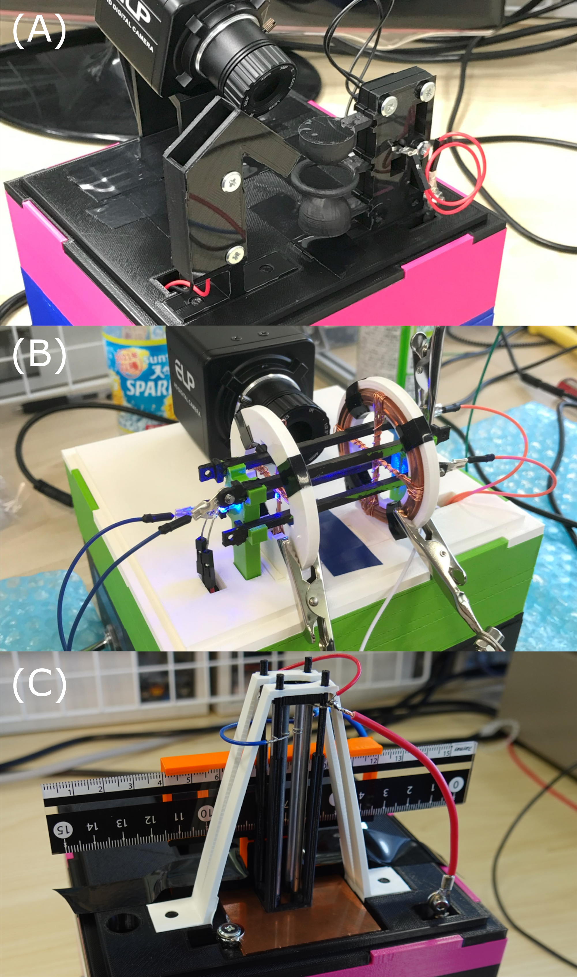
Figure 1: Photo of three Paul trap modules. (A) ring-type, (B)Linear-type parallel to the ground (vertical-linear-type), (C)Linear-type perpendicular to the ground (horizontal-linear-type). (A) and (C) are used for the measurement of the charge-to-mass ratio.

1. measurement of applied AC Voltage conditions that can trap particles using the ring-type.

2. balance between the gravity and Coulomb force the DC electric field using the vertical-linear-type.

3. measurement of the amplitude of forced oscillation by applying an external oscillation field using the vertical-linear-type.

2 Principle of the Paul trap

Two types of Paul traps were used in this experiment: (1)a Paul trap that generates a rotating hyperbolic potential (ring type) and (2) a Paul trap that confines only the $x,y$ directions (vertical linear type).

The motion of the charged particles in the Paul trap obeys the Mathieu equation. Consider the equations of motion for trapped particles of mass $m$ and charge $Q$: The electrode shown in Fig. 2 is a rotational hyperbolic potential

$$\phi=\frac{\phi_{0}}{2r_{0}^{2}}(x^{2}+y^{2}-2z^{2})=\frac{\phi_{0}}{2r_{0}^{2}}(r^{2}-2z^{2})$$

$$\phi_{0}=V_{\rm DC}+V_{\rm AC}\cos(\Omega t).$$

Here, $V_{\rm DC},V_{\rm AC}$ are the DC and AC voltages applied to the electrodes, respectively; $\Omega$ is the angular frequency of the AC voltage. The equation of motion for the trapped ions is

$$r \colon \hskip 2.0ptm\derivative[2]{r}{t} =-\frac{Q}{r_{0}^{2}}\left[V_{DC}+V_{AC}\cos(\Omega t)\right]r$$

$$z \colon \hskip 2.0ptm\derivative[2]{z}{t} =\frac{2Q}{r_{0}^{2}}\left[V_{DC}+V_{AC}\cos(\Omega t)\right]z.$$

using the dimensionless quantity $\tau=\Omega t/2$.

$$\derivative[2]{u}{\tau}+\left[a_{u}-2q_{u}\cos(2\tau)\right]u=0\quad(u=r,z)$$ (1)

$$a_{z}=-\frac{Q}{m}\frac{8V_{\rm DC}}{r_{0}^{2}\Omega^{2}}=-2a_{r}$$

$$q_{z}=\frac{Q}{m}\frac{4V_{\rm AC}}{r_{0}^{2}\Omega^{2}}=-2q_{r},$$

where $a,q$ are dimensionless quantities that depend on the charge-to-mass ratio of the charged particles. Equation (1) is the Mathieu Equation and is characterized by the values of the dimensionless quantities $a,q$ that determine the stability of the trap (Fig. 3).

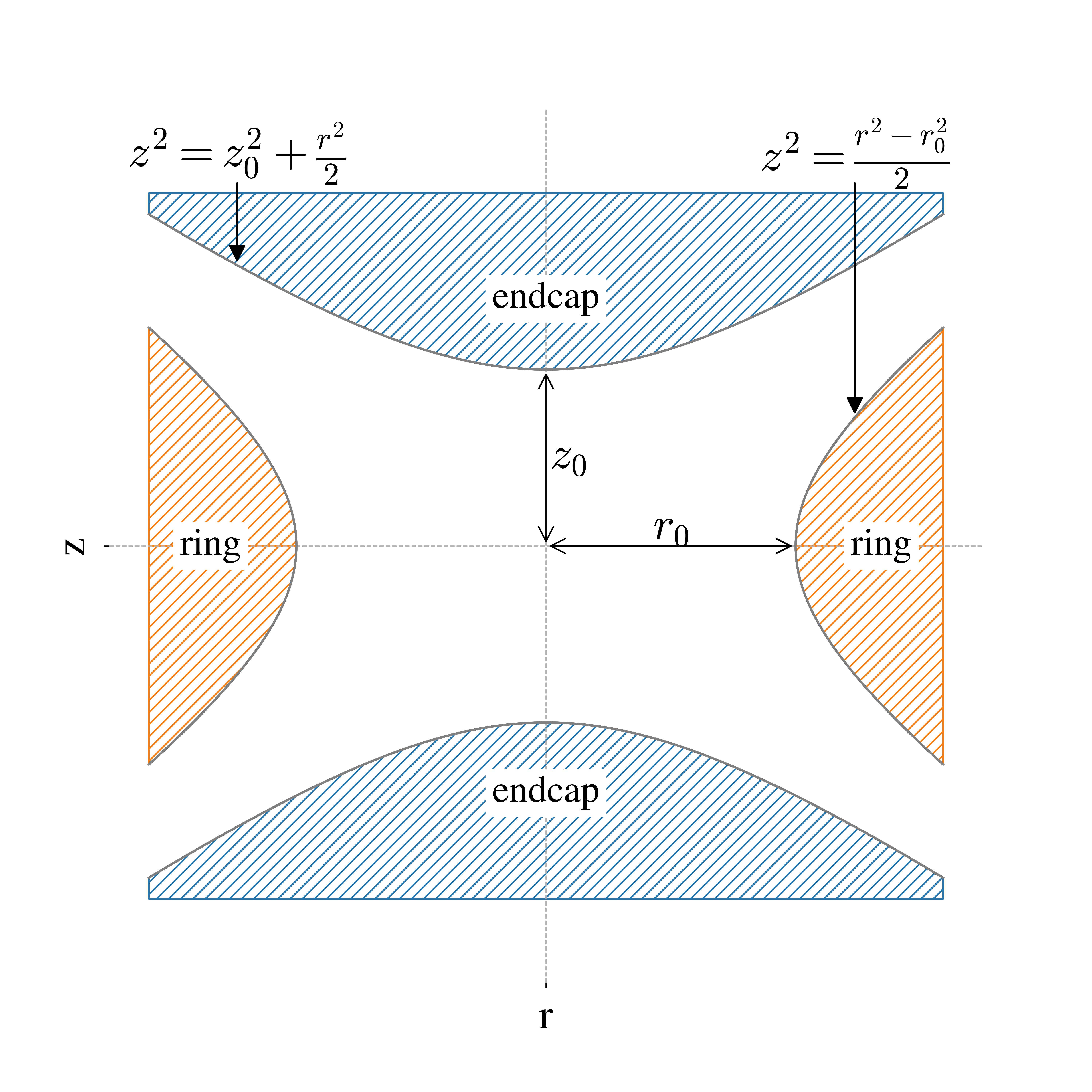
Figure 2: Schematic of a ring-type Paul trap electrode. There is a relationship $r_{0}^{2}=2z_{0}^{2}$ between $r_{0}$ and $z_{0}$.

Figure 3: Stability diagram for Mathieu equation. The shaded area is the stability region.

The viscous and inertial forces of air should be considered when particles are trapped in the air. The size of the Lycopodium spores [2] used as trapped particles in this experiment was

$$D=2R =26.0\pm 2.5\ {\rm\mu m}$$

$$\rho =510\pm 40\ {\rm kg/m^{3}}.$$

Therefore, the Reynolds number $R_{e}$ of Lycopodium spores is

$$R_{e}=\frac{\rho_{\rm air}vD}{\eta}\approx 1.7\times 10^{-5}\ll 1$$

where the density of air is $\rho_{\rm air}=1.21\ {\rm kg/m^{3}}$, dynamic viscosity is $\eta=1.82\times 10^{-5}\ {\rm Pa\cdot s}$ and velocity of the particle is $v=10^{-6}\sim 10^{-4}\ {\rm m/s}$. Thus, the viscous force is dominant over the inertial force in the case of these spores. Therefore, Eq. (1), with the coefficient of the viscous resistance as $k$, is

$$\derivative[2]{u}{\tau}+b\derivative{u}{\tau}+\left[a_{u}-2q_{u}\cos(2\tau)\right]u=0\quad(u=r,z)$$ (2)

$$b=\frac{2k}{m\Omega}.$$

Furthermore, assuming that the particles are spherical, the proportionality coefficient $k$ can be rewritten as $6\pi\eta R$ from Stokes’ law, and the mass of the particles as $m=4/3\pi R^{3}\rho$, the dimensionless quantity $b$ is

$$b=\frac{9\eta}{R^{2}\rho\Omega}.$$

3 Designing the Paul trap

The device was divided into two components: a power supply module and an electrode module. The power supply module contained a 60-fold high-voltage transformer (UFO-6K-001-P100,UNION ELECTRIC) and raised the voltage from that of a household power supply in Japan (100 V / 50 or 60 Hz) to 6000 V. The electrode modules (ring-type, two linear types) were switchable for each measurement. Each part was fabricated using a 3D printer (Ultimaker S3) and polylactic acid (PLA) filament. The trapped particles were observed using a mounted USB webcam.

The ring-type trap comprises two hemispheres and a ring electrode (Fig. 4). This type applies only an AC voltage ($V_{\rm DC}=0$); hence, $a=0$,

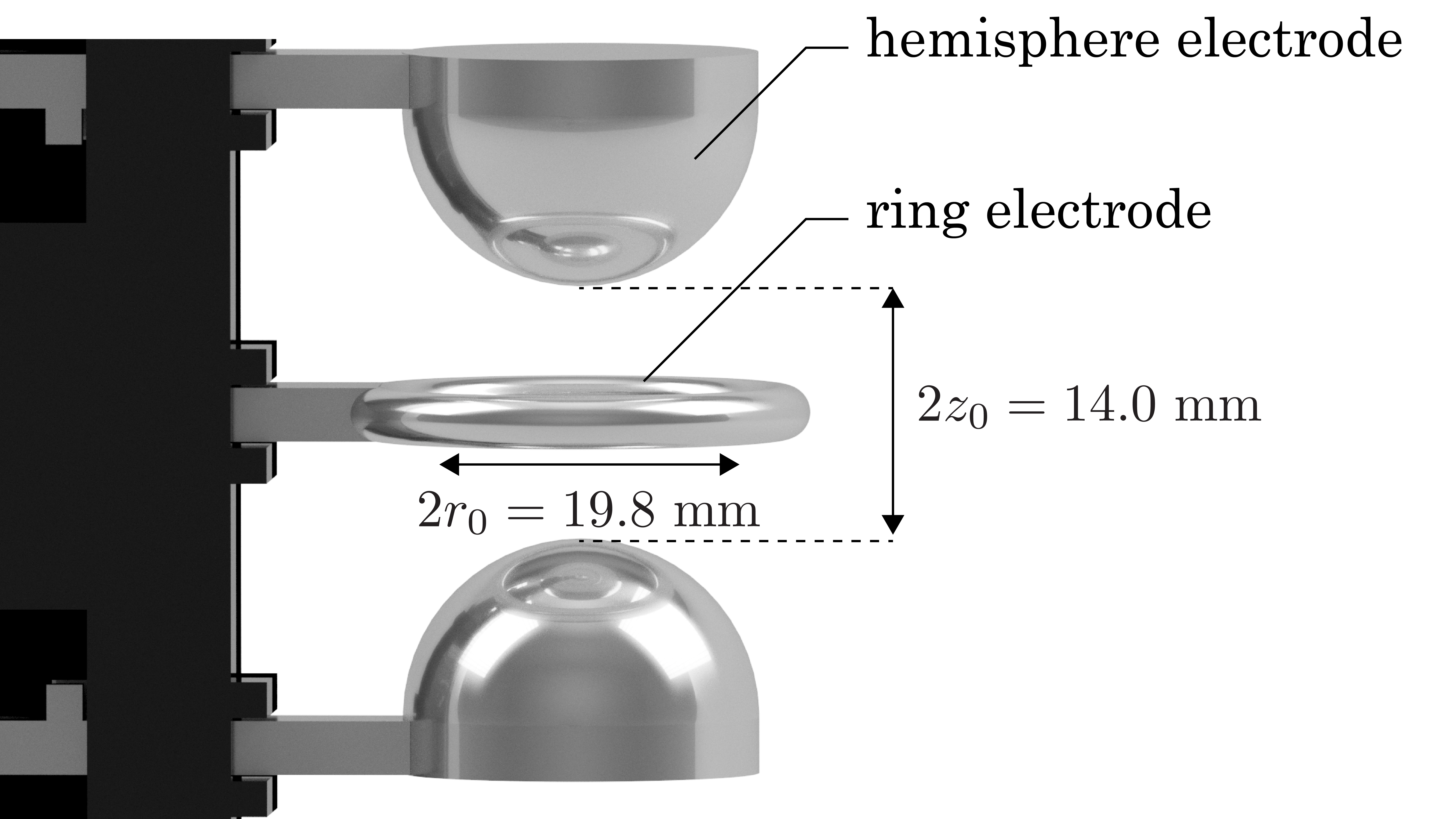
Figure 4: Three-dimensional model of attachable electrodes of the ring-type trap.

The vertical linear type comprises four rods for AC voltage and one bottom plate for DC voltage (Fig. 5).

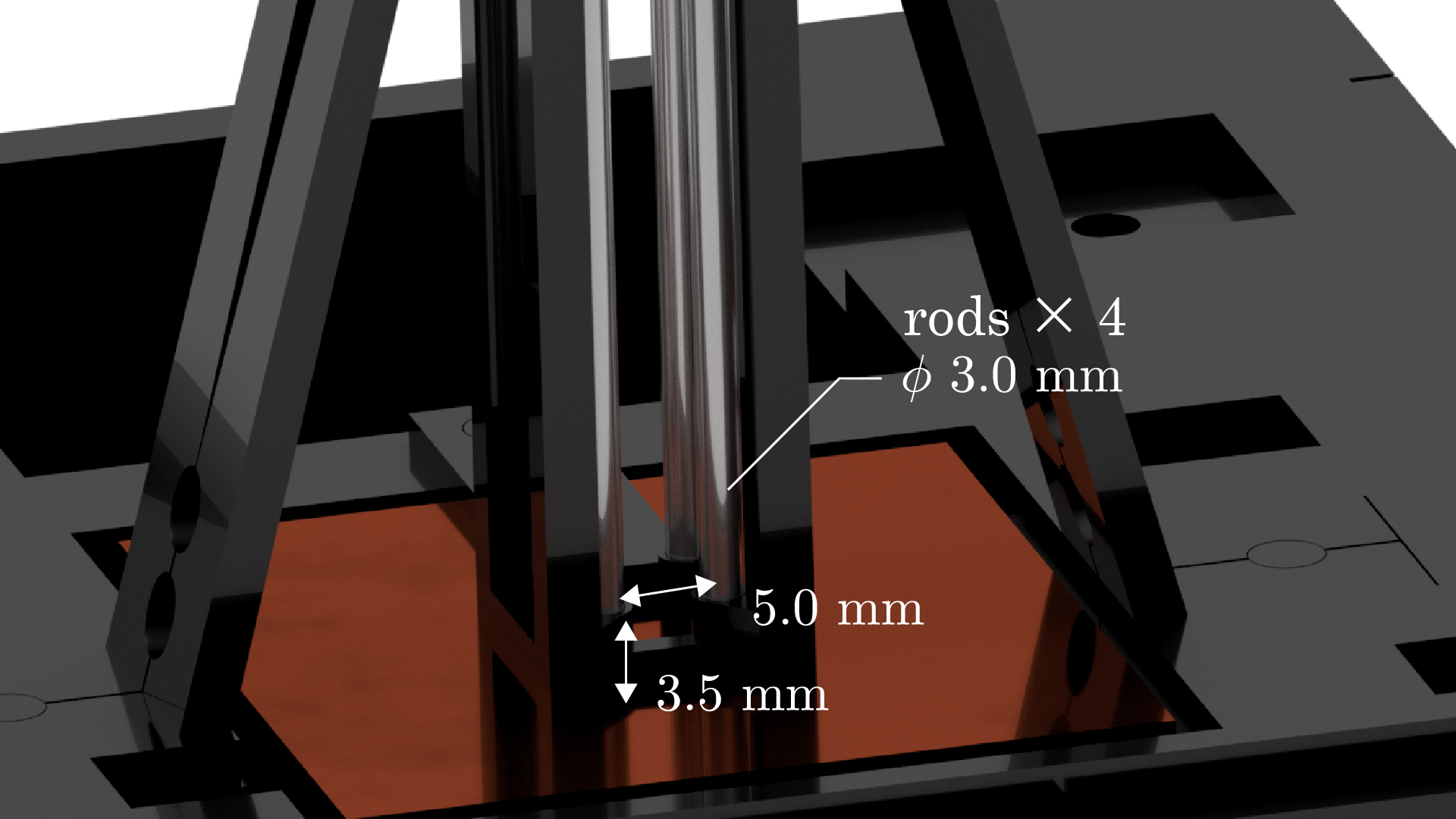
Figure 5: Three-dimensional model of attachable electrodes of vertical-linear-type trap.

Lycopodium spores, which are easily available spherical plant particles, were used as trap particles(Fig. 6).

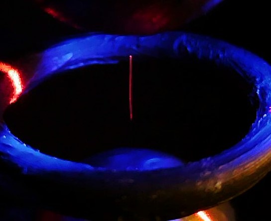
Figure 6: Observed trajectory of particles. Due to the refresh rate of the webcam (30 Hz), the trajectory is seen as a line.

4 Measurement of charge-to-mass ratio

4.1 Applied AC Voltage conditions that can trap particles using the ring-type Paul trap

According to Eq. (1) and (2), the trap condition is determined by $q$ and air resistance coefficient $b$. By obtaining the maximum values of $q$ and $V_{\rm AC}$ under stable trapping conditions ($q_{\rm{max}}$ and $V_{\rm AC}^{\rm max}$), the charge-to-mass ratio of the particles $Q/m$ can be calculated using the following equation:

$$\frac{Q}{m}=\frac{r_{0}^{2}\Omega^{2}}{4}\frac{1}{V_{\rm AC}^{\rm max}}q_{\rm max}.$$

$q_{\rm{max}}$ is calculated using the Runge-Kutta method as shown in Table 1 and the following equation, which considers the gravitational force in Eq. 2

$$\derivative[2]{r}{\tau}+b\derivative{r}{\tau}+\left[a_{r}-2q_{r}\cos(2\tau)\right]r=0$$

$$\derivative[2]{z}{\tau}+b\derivative{z}{\tau}+\left[a_{z}-2q_{z}\cos(2\tau)\right]z+\frac{4g}{\Omega^{2}}=0.$$

The calculated $q_{\rm{max}}$ is:

$$q_{\rm{max}}=17\pm 4$$

Table 1: Parameters to calculate the stability condition of the trap.

Parameter	Value
$r_{0}$	$9.9\pm 0.5\ {\rm mm}$
$\Omega$	$2\pi\times 50\ {\rm Hz}$
$\eta$	$1.81920(6)\times 10^{-5}\ {\rm Pa\cdot s}$
$R$	$13.0\pm 1.3\ {\rm\mu m}$
$\rho$	$510\pm 40\ {\rm kg/m^{3}}$

A single particle was trapped with a ring-type Paul trap, and we gradually raised the applied voltage $V_{\rm{AC}}$ to escape. The obtained maximum $V_{\rm{AC}}$ under the trap conditions is

$$V_{\rm{AC}}^{\rm max}=2.5\pm 0.8\ \rm{kV}.$$

From $q_{\rm{max}}$ and $V_{\rm AC}^{\rm max}$, $Q/m$ can be calculated as:

$$\frac{Q}{m}=(1.7\pm 0.7)\times 10^{-2}\ \rm{C/kg}.$$

4.2 Applied AC Voltage conditions that can trap particles using the vertical-linear-type Paul trap

The gravitational and Coulomb forces from the bottom plate are balanced in the $z$ direction with a vertical-linear-type trap as

$$mg=QE_{\rm DC}$$

Thus, the charge-to-mass ratio is calculated as follows:

$$\frac{Q}{m}=\frac{g}{E_{\rm DC}}.$$ (3)

A single particle is trapped in a vertical-linear-type trap under the condition of $V_{\rm{AC}}=2100$ V, $V_{\rm{DC}}=-80\sim-150$ V where $V_{\rm{DC}}$ is static applied voltage to the bottom plate. Subsequently, particle displacement was measured according to the increase in $V_{\rm{AC}}$ (Fig. 8).

The distribution of the static electric field was calculated using the Statics / Low-frequency Solver from CST Studio Suite (Fig. 7) and fitted the distribution on $z$ axis by the exponential function $E_{\rm{DC}}(z)=Az\exp\quantity(-z/L)+C$ to obtain electric field strength on each particle’s positions.

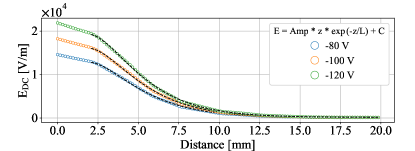
Figure 7: Electric field strength on $z$ axis with applied static voltage $E_{\rm{DC}}=-80,-100,-120$ V calculated using CST Studio. The distribution on the $z$ axis was fitted by the exponential function $E_{\rm{DC}}(z)=Az\exp\quantity(-z/L)+C$ to obtain electric field strength on each particle’s positions.

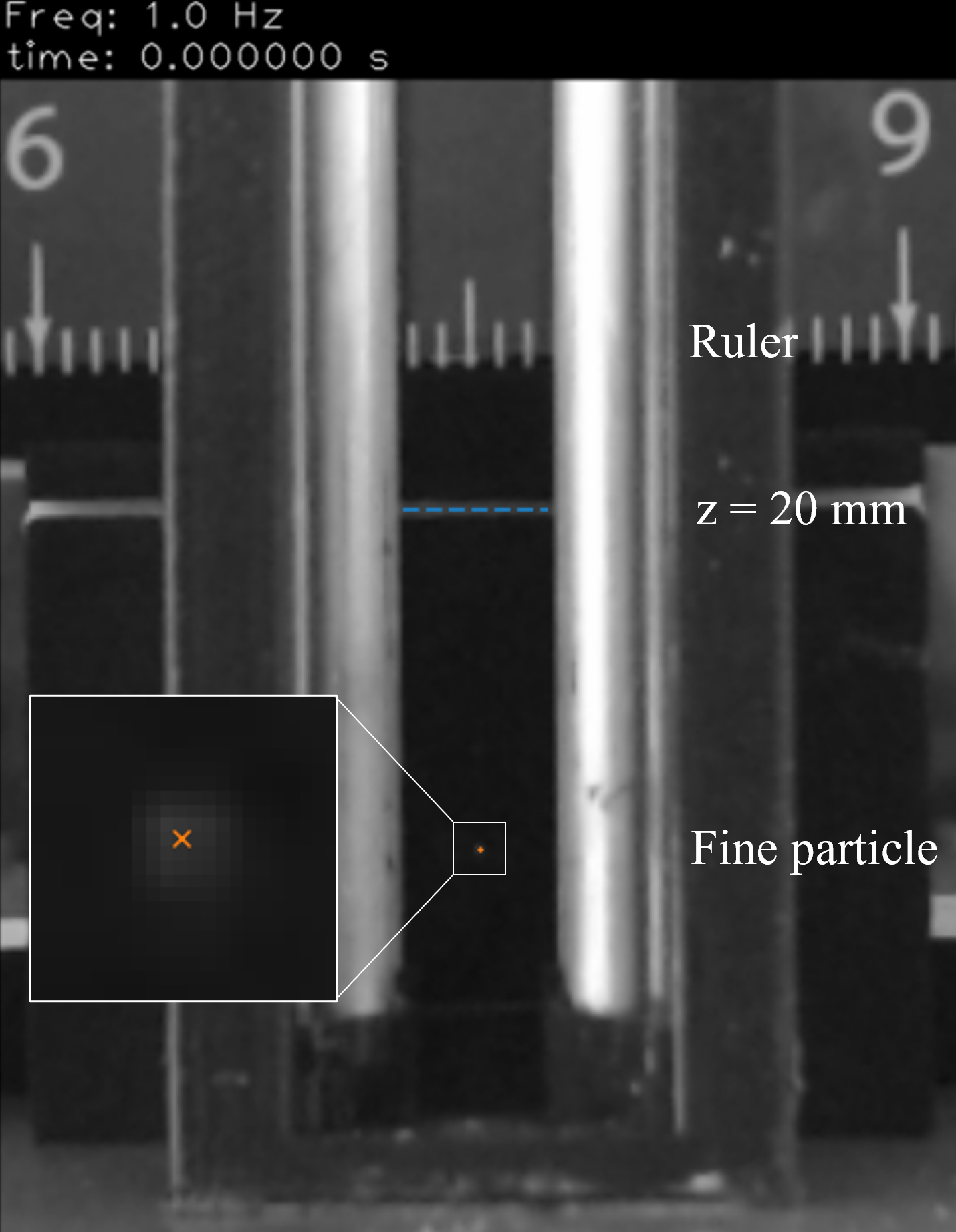
Figure 8: Observed image of a particle trapped by the vertical-linear-type Paul trap. Positions of the particle are measured with reference to the line ($z=20$ mm) and ruler in this view.

Figure 9 shows the relationship between the particle displacement and $V_{\rm{DC}}$. The charge-to-mass ratio ($Q/m$) calculated using Eq.3 for each $V_{\rm{DC}}$ (Fig. 10) and the weighted average value is

$$\frac{Q}{m}=(8.2\pm 0.1)\times 10^{-4}\ {\rm C/kg}.$$

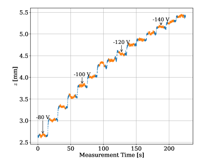
Figure 9: Position change of the particle by the applied static voltage $V_{\rm{DC}}$.

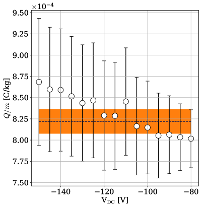
Figure 10: Calculated charge-to-mass ratio ($Q/m$) by each applied static voltage $V_{\rm{DC}}$.

4.3 Amplitude of forced oscillation by applying an external oscillation field using the vertical linear type.

Applying a slow (sub-Hz) oscillating electric field ($E_{\rm AC}\sin(\omega t)$) causes forced oscillation as

$$m\derivative[2]{z}{t} =-k\derivative{z}{t}+QE_{\rm AC}\sin(\omega t),$$

$$z =A\sin(\omega t+\phi)$$

where the amplitude $A$ is as follows:

$$A =\frac{QE_{\rm AC}}{k\omega}\left[1+\quantity(\frac{m\omega}{k})^{2}\right]^{-\frac{1}{2}}$$

$$\approx\frac{Q}{m}\frac{mE_{\rm AC}}{k}\frac{1}{\omega}\quad\quantity(\because\frac{m\omega}{k}\ll 1)$$

$$=\frac{Q}{m}\frac{2R^{2}\rho E_{\rm AC}}{9\eta}\frac{1}{\omega}.$$ (4)

Thus, the charge-to-mass ratio ($Q/m$) can be obtained by measuring $A$ for each $\omega$. Figure 11 shows the measured $A$ values for $V_{\rm{AC}}=10,20,30,40,50\rm{V}$. Fitted by Eq. 4 for the result of each $V_{\rm{AC}}$ to obtain charge-to-mass ratio ($Q/m$) for each $V_{\rm{AC}}$ (Fig. 12) and weighted averaged these values as

$$\frac{Q}{m}=(3.4\pm 0.3)\times 10^{-3}\ \rm{C/kg}.$$

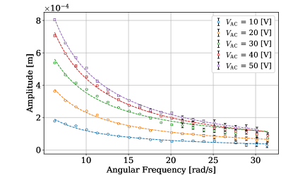
Figure 11: Amplitudes of forced oscillation with several applied oscillation voltages $V_{\rm{AC}}$ and frequencies. Amplitudes are inversely proportional to the frequency of applied oscillation fields according to Eq. 4.

Figure 12: Calculated charge-to-mass ratio ($Q/m$) by each applied static voltage $V_{\rm{AC}}$.

5 Conclusion

We developed a tabletop Paul trap that can be replaced with two attachable traps, ring- and linear-type, and measured the charge-to-mass ratio of trapped particles using three different techniques. This tabletop Paul trap operates on a household power supply only, and by connecting the built-in camera to a PC via USB, measurements and image analysis can be performed safely in a typical school environment. Therefore, it was shown that these three charge-to-mass ratio measurements could be safely performed in an experimental school class.

The results varied in the range of $Q/m=10^{-2}$ to $10^{-3}$ C/kg, consistent with the typical value for charged Lycopodium spores [2]. The uncertainties in the value arise from variations in spore size and structure, as well as the charging method which involves rubbing a Teflon rod with cloth and then attaching the spores to it

In the case of the ring-type charge-to-mass ratio measurement, it is necessary to determine the particle size and maximum value of the trap stability condition $q_{\rm{max}}$ from numerical calculations. To measure the charge-to-mass ratio in the vertical linear type, it is necessary to determine the distribution of the electric field on the axis with respect to the applied voltage. In the case of vertical linear-type measurements using AC voltage application, the particle size and density should be determined in advance. As the electric field distribution can be calculated in advance at the time of production, the simplest method for particles of unknown diameter and density is to experiment with a vertical-linear-type DC voltage application.

Trap devices have been used in several cases in Japan, such as in a class at Waseda University Honjo Senior High School, booth exhibition at the Sendai Science Museum, and open- campus exhibition at the University of Tokyo, mainly for high school students. In particular, at Waseda University Honjo Senior High School, traps have been used in demonstration classes conducted by high school teachers and in year-long exploratory activities conducted by students.

6 Acknowledgement

This research was partially supported by the Mitsubishi Memorial Foundation for Educational Excellence, the Cyclotron Radioisotope Center at Tohoku University, and the Leave a Nest grant incu $\cdot$ be award.

References

- [1] H. Kobayashi et al. Making an ion trap for student’s experiment. Physics Education Society of Japan, Vol. 44, No. 4, pp. 385–388, 1996.
- [2] Kenneth G. Libbrecht and Eric D. Black. Improved microparticle electrodynamic ion traps for physics teaching. American Journal of Physics, Vol. 86, No. 7, pp. 539–558, 2018.
- [3] Dührkoop S. Jansky A. Keller O. Lorenz A. Schmeling S. … Woithe J.McGinness. 3d-printable model of a particle trap: Development and use in the physics classroom. Journal of Open Hardware, Vol. 3, No. 1, p. 1, 2019.