Efficient Reinforcement Learning for Jumping Monopods

Abstract

In this work, we consider the complex control problem of making a monopod reach a target with a jump. The monopod can jump in any direction and the terrain underneath its foot can be uneven. This is a template of a much larger class of problems, which are extremely challenging and computationally expensive to solve using standard optimisation-based techniques. Reinforcement Learning (RL) could be an interesting alternative, but the application of an end-to-end approach in which the controller must learn everything from scratch, is impractical. The solution advocated in this paper is to guide the learning process within an RL framework by injecting physical knowledge. This expedient brings to widespread benefits, such as a drastic reduction of the learning time, and the ability to learn and compensate for possible errors in the low-level controller executing the motion. We demonstrate the advantage of our approach with respect to both optimization-based and end-to-end RL approaches.

I Introduction

Legged robots have become a popular technology to navigate unstructured terrains, but are complex devices for which control design is not trivial. Remarkable results have been reached for locomotion tasks like walking and trotting [1]. Other tasks, like performing jumps, are more challenging because even small deviations from the desired trajectory can have a large impact on the landing location and orientation [2]. This problem has received some attention in the last few years. A line of research has produced heuristic approaches relying on physical intuitions and/or on simplified models to be used in the design of controllers or planners [3, 4]. However, the hand-crafted motion actions produced by these approaches are not guaranteed to be physically implementable. Another common approach is to use full-body numerical optimisation [5]. Very remarkable is the rich set of aerial motions produced by MIT Mini Cheetah in [6, 7, 8] using a centroidal momentum-based nonlinear optimisation. A problem with optimisation-based approaches on high dimensional nonlinear problems is the high computational cost, which makes them unsuitable for a real-time implementation, especially to replan trajectories over a receding horizon. Recent advances [9, 5] have brought to significant improvements in the efficiency of Model Predictive Control (MPC) for jumping tasks. However, the price to pay is to introduce some artificial constraints such as fixing the contact sequence, the time-of-flight, or optimising the contact timings offline.

A third set of approaches is based on Reinforcement Learning (RL). The seminal work of Lillicrap [10] showed that a Deep Deterministic Policy Gradient (DDPG) algorithm combined with a Deep Q network could be successfully applied to learn end-to-end policies for a continuous action domain, using an actor-critic setting. In view of these results, several groups have then applied RL to quadrupeds for locomotion tasks [11, 12, 13, 14, 15], and to in-place hopping legs [16]. As with most of model-free reinforcement approaches, DDPG requires a large number of training steps (on the order of millions) to find good solutions. Other approaches [17, 18, 19] seek to improve the efficiency and the robustness of the learning process by combining Trajectory Optimization (TO) with RL: they use the former to generate initial trajectories to bootstrap the exploration of alternatives made by the latter.

As a final remark, the efficiency and the robustness of the RL learning process is heavily affected by a correct choice of the action space [20, 21]. Some approaches require that the controller directly generates the torques [22], while others suggest that the controller should operate in Cartesian or joint space  [12, 23].

Paper Contribution. This work proposes an RL framework capable of producing an omni-directional jump trajectory (from standstill) on uneven terrain, computed within a few milliseconds, unlocking real-time usage with the current controller rates (e.g. in the order of $kHz$). The main objective of this paper is to reduce the duration of the learning phase without sacrificing the system’s performance. A reduced length of the learning phase has at least two indisputable advantages: lowering the barriers for the access to this technology for professionals and companies with a limited availability of computing power, and addressing the environmental concerns connected with the carbon footprint of learning technologies [24].

Our strategy is based on the following ideas: first, learning is performed in Cartesian space rather than in joint space so that the agent can more directly verify the effect of its actions. Second, we notice that while the system is airborne, its final landing point are dictated by simple mechanical laws (ballistic). Therefore, the learning process can focus solely on the thrusting phase. Third, we know from biology [25] that mammals are extremely effective in learning how to walk because of ”prior” knowledge in their genetic background. This means that the learning process can be guided by an approximate knowledge of what the resulting motion should ”look like”. Specifically, we parametrise the thrusting trajectory (i.e. from standstill to lift-off) for the Center of Mass (CoM) with a ($3^{rd}$ order) Bezier curve. This choice of a Bezier curve to parametrize the action space is not uncommon in the literature [26], [27], [28], and in our case is motivated by the physical intuition that a jump motion, to exploit the full joint range, needs a ”charging” phase to compress the legs followed by an extension phase where the CoM is accelerated both upwards and in the jump direction. Clearly, by making this restriction, we prevent the learning phase from exploring alternative options. However, as we will see in the paper, the final result is very close to optimal and the system retains good generalisation abilities.

Our approach is based on TD3, a state-of-the-art Deep Reinforcement Learning (Deep-RL) algorithm [29] trained to minimise a cost very similar to the ones typically used in optimal control. The Cartesian trajectory generated by our RL agent is translated into joint space via inverse kinematics, and tracked by a low-level joint-space Proportional-Derivative (PD) controller with gravity compensation. Our results reveal that possible inaccuracies in the controller can be learned and compensated by the RL agent. In this paper we do not focus on the landing phase, which we assume to be managed by a different controller, such as [2]. We compare our approach (that we will call Guided Reinforcement Learning (GRL)) with both a baseline TO controller with a fixed duration of the thrusting phase, and a ”standard” End-to-end Reinforcement Learning (E2E) (which considers joint references as action space). In the first case, we achieved better or equal performance, and a dramatic reduction in the online computation time. With respect to E2E locomotion approaches [22, 12], we observed a substantial reduction in the number of episodes (without considering parallelization) needed to achieve good learning performances. Instead, an E2E implementation specific for a jump motion (Section IV-2), did not provide satisfactory learning results.

The paper is organized as follows: Section II presents the GRL approach, detailing the core components of the MDP (action, reward functions). Section III provides implementation details. In Section IV we showcase our simulation results comparing with state-of-the-art approaches. Finally, we draw the conclusions in Section V.

II Problem description and solution overview

Simple notions of bio-mechanics suggest that legged animals execute their jumps in three phases: 1. thrust: an initial compression is followed by an explosive extension of the limbs in order to gain sufficient momentum for the lift-off; the phase finishes when the foot leaves the ground; 2. flight: the body, subject uniquely to gravity, reaches an apex where the vertical CoM velocity changes its sign and the robot adjusts its posture to prepare for landing; 3. landing: the body realizes a touch-down, which means that the foot establishes again contact with the ground. For the sake of simplicity, we consider a simplified and yet realistic setting: a monopod robot, whose base link is sustained by passive prismatic joints preventing any change in its orientation (see Section III-C). The extension to a full quadruped (which requires considering also angular motions) is left for future work. In this paper, we focus on the thrust phase. The flight phase is governed by the ballistic law. Let $\mathbf{c}_{tg}$ be the target location and let the CoM state at lift-off be $(\mathbf{c}_{lo},\mathbf{\dot{c}}_{lo})$. After lift-off, the trajectory lies on the vertical plane containing $\mathbf{c}_{lo}$ and $\mathbf{c}_{tg}$. The set of possible landing CoM positions are function of $\mathbf{c}_{lo}$, $\mathbf{\dot{c}}_{lo}$ and are given by the following equation:

$$\begin{cases}\mathbf{c}_{tg,xy}=\mathbf{c}_{lo,xy}+\mathbf{\dot{c}}_{lo,xy}T_{fl}\\ \mathbf{c}_{tg,z}=\mathbf{c}_{lo,z}+\mathbf{\dot{c}}_{lo,z}T_{fl}+-\frac{1}{2}gT_{fl}^{2}\end{cases}$$ (1)

where $T_{fl}=(\mathbf{c}_{tg,xy}-\mathbf{c}_{lo,xy})/\mathbf{\dot{c}}_{lo,xy}$ is the flight time. In this setting, our problem can be stated as follows:

Problem 1

Synthesise a thrust phase that produces a lift-off configuration (i.e. CoM position and velocity) that: 1. satisfies (1), 2. copes with the potentially adverse conditions posed by the environment (i.e. contact stability, friction constraints), 3. satisfies the physical and control constraints.

Nonlinear optimisation is frequently used for similar problems. However, it has two important limitations that discourage its application in our specific case: 1. the computation requirements are very high, complicating both the real–time execution and the use of low–cost embedded hardware, 2. the problem is strongly non-convex, which can lead the solvers to local minima.

II-A Overview of the approach

In this work, we use RL to learn optimal joint trajectories to realise a jump motion, that is then tracked by a lower-level controller. We adopted the state-of-the-art Twin Delayed Deep Deterministic Policy Gradient (TD3), a Deep-RL technique. This algorithm is based on the well-known Actor-Critic architecture. The main idea behind TD3 is to adopt two Deep Neural Network (NN) to approximate the policy, represented by the Actor, and two Deep NN to approximate the action-value function, represented by the Critic.

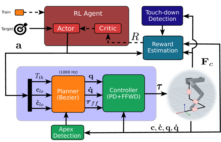
Figure 1: Diagram of the RL Framework. The framework is split into two levels: the RL agents and the planner. The RL agent produces an action for the planner, based on a desired target. This computes a Bezier reference curve that is mapped into joint motion via inverse kinematics and tracked by the PD controller that provides the joint torques to feed the robot. During the training, at the end of each episode a reward is computed and fed back to the RL agent.

Our RL pipeline is depicted in Fig. 1.

III Design and implementation of the RL agent

Based on the discussion in the previous section, the thrust phase is characterised by the lift-off position $\mathbf{c}_{lo}$ and velocity $\mathbf{\dot{c}}_{lo}$ and by the thrust time $T_{th}$ which is the time spent to reach the lift-off configuration from the initial state. The state of the environment is defined as ($\mathbf{c}$, $\mathbf{c}_{tg}$) where $\mathbf{c}\in\mathbb{R}^{3}$ is the CoM position and $\mathbf{c}_{tg}\in\mathbb{R}^{3}$ the CoM at the landing location (target). The objective of the RL agent is to find the jump parameters ($\mathbf{c}_{lo}$, $\mathbf{\dot{c}}_{lo}$, $T_{th}\in\mathbb{R}$), that minimise the landing error at touch-down $\|\mathbf{c}-\mathbf{c}_{tg}\|$ while satisfying the physical constraints. Our jumping scenario thought can be seen as a single-step trajectory where the only action performed leads always to the end state.

III-A The Action Space

The dimension of the action space has a strong impact on the performance of the RL algorithm. Indeed, a NN with a smaller number of outputs is usually faster to train. What is more, a smaller action space reduces the complexity of the mapping, speeding up the learning process.

A first way to reduce the complexity of the action space is by expressing $\mathbf{c}_{lo}$ and $\mathbf{\dot{c}}_{lo}$ in spherical coordinates. Because of the peculiar nature of a jump task, the trajectory lies in the plane containing the CoM $\mathbf{c}$ and its desired target location $\mathbf{c}_{tg}$. Hence, the yaw angle $\varphi$ remains constant ($\bar{\varphi}$) throughout the flight and we can further restrict the coordinates to a convex bi-dimensional space:

$$\small\begin{cases}\mathbf{c}_{lo,x}=r~{}\cos(\theta)\cos(\bar{\varphi})\\ \mathbf{c}_{lo,y}=r~{}\cos(\theta)\sin(\bar{\varphi})\\ \mathbf{c}_{lo,z}=r~{}\sin(\theta)\end{cases}\begin{cases}\mathbf{\dot{c}}_{lo,x}=r_{v}~{}\cos(\theta_{v})\cos(\bar{\varphi})\\ \mathbf{\dot{c}}_{lo,y}=r_{v}~{}\cos(\theta_{v})\sin(\bar{\varphi})\\ \mathbf{\dot{c}}_{lo,z}=r~{}\sin(\theta_{v})\end{cases}$$ (2)

As shown in Fig. 2, the lift-off position $\mathbf{c}_{lo}$ is identified by: the radius $r$ (i.e., the maximum leg extension), the yaw angle $\varphi$ and the pitch angle $\theta$. Likewise, the lift-off velocity $\dot{c}_{lo}$, is described by its magnitude $r_{v}$, and the pitch angle $\theta_{v}$ with respect to the ground.

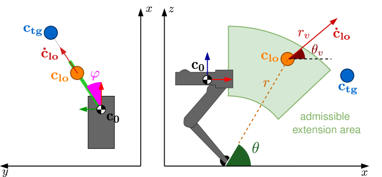
Figure 2: Action parametrization and its bounds. On the left the top view, on the right the side view of the jumping plane.

Therefore, by using this assumption, we have reduced the dimension of the action space from $7$ to $5$: $\mathbf{a}=(T_{th},r,\theta,r_{v},\theta_{v})\in\mathbb{R}^{5}$.

The action space can be further restricted by applying some domain knowledge. The radius $r$ has to be smaller than a value $r_{max}$ ($0.32$ $m$) to prevent boundary singularity due to over-extension, and greater than a value $r_{min}$($0.25$ $m$) to avoid complete leg retraction. The bounds on the velocity $\dot{c}_{lo}$, represented by $r_{v}\in\left[0.1,4\right]$ $m/s$, and $\theta_{v}\in\left[\frac{\pi}{6},\frac{\pi}{2}\right]$ $rad$, and the bounds on pitch angle $\theta\in\left[\frac{\pi}{4},\frac{\pi}{2}\right]$ $rad$ are set to rule out jumps that involve excessive foot slippage and useless force effort. Specifically, restricting to a positive $\theta_{v,min}$ ensures a non-negligible vertical component for the velocity, while bounding $\theta_{v}$ to the positive quadrant secures that the lift-off velocity be oriented ”toward” the target.

III-A1 Trajectory Parametrisation in Cartesian Space

Our strategy to tackle the problem of generating a compression-extension trajectory for the leg, to achieve a given lift-off configuration $\mathbf{c}_{lo}$, is based on two important choices: 1. making the RL agent learn the trajectory in Cartesian Space and then finding the joint trajectories through inverse kinematics, 2. restricting the search of the Cartesian space evolution to curves generated by known parametric functions. This has the aim to reduce the search space and simplifying convergence.

The analytical and geometric properties of $3^{rd}$ order Beziér curves make them a perfect fit for our problem. A $3^{rd}$ order Bèzier curve is defined by four control points. In our case, the first and the final points are constrained to be the initial and final CoM positions, respectively. The derivative of a $3^{rd}$ degree Bèzier curve is itself a Bèzier curve of $2^{nd}$ degree with 3 control points defined as $3(\mathbf{P}_{i+1}-\mathbf{P}_{i})$. The curve domain is defined only in the normalised time interval: $t\in\begin{bmatrix}0,1\end{bmatrix}$. Defining the following Bernstein polynomials:

$$\bm{\eta}(t)=\begin{bmatrix}(1-t)^{3}&3(1-t)^{2}t&3(1-t)t^{2}&t^{3}\end{bmatrix}^{T}$$ (3)

$$\bm{\dot{\eta}}(t)=\begin{bmatrix}(1-t)^{2}&2(1-t)t&t^{2}\end{bmatrix}^{T}$$ (4)

we can compactly write the Beziér curve as function of its $\mathbf{P}_{i}\in\mathbb{R}^{3}$ control points:

$$\mathbf{c}=\begin{bmatrix}\mathbf{P}_{0}&\mathbf{P}_{1}&\mathbf{P}_{2}&\mathbf{P}_{3}\end{bmatrix}\bm{\eta}(t)$$ (5)

Since we are considering an execution time $T_{exe}\in\begin{bmatrix}0,T_{th}\end{bmatrix}$ and $t=\frac{T_{exe}}{T_{th}}$, then the derivative writes:

$$\mathbf{\dot{c}}=\frac{1}{T_{th}}\begin{bmatrix}\mathbf{P}^{\prime}_{0}&\mathbf{P}^{\prime}_{1}&\mathbf{P}^{\prime}_{2}\end{bmatrix}\bm{\dot{\eta}}(t)$$ (6)

From the definition of the curve (5) and its derivative (6), we can compute the control points $\mathbf{P}_{i}$ by setting the boundary conditions of the initial/lift-off CoM position $\mathbf{c}_{0}$, $\mathbf{c}_{lo}$ and initial/lift-off CoM velocity $\mathbf{\dot{c}}_{0}$,$\mathbf{\dot{c}}_{lo}$ in (7).

$$\small\begin{cases}\begin{aligned} {\mathbf{P}}^{\prime}_{0}&=\frac{3}{T_{th}}(\mathbf{P}_{1}-\mathbf{P}_{0})\\ &=\mathbf{\dot{c}}_{0}=\mathbf{0}\\ {\mathbf{P}}^{\prime}_{1}&=\frac{3}{T_{th}}(\mathbf{P}_{2}-\mathbf{P}_{1})\\ {\mathbf{P}}^{\prime}_{2}&=\frac{3}{T_{th}}(\mathbf{P}_{3}-\mathbf{P}_{2})\\ &=\mathbf{\dot{c}}_{lo}\end{aligned}\end{cases}\begin{cases}\begin{aligned} \mathbf{P}_{0}&=\mathbf{c}_{0}\\ \mathbf{P}_{1}&=\frac{T_{th}}{3}{\mathbf{P}}^{\prime}_{0}+\mathbf{P}_{0}\\ &=\frac{T_{th}}{3}\mathbf{\dot{c}}_{0}+\mathbf{c}_{0}\\ \mathbf{P}_{2}&=-\frac{T_{th}}{3}{\mathbf{P}}^{\prime}_{2}+\mathbf{P}_{3}\\ &=-\frac{T_{th}}{3}\mathbf{\dot{c}}_{lo}+\mathbf{c}_{lo}\\ \mathbf{P}_{3}&=\mathbf{c}_{lo}\\ \end{aligned}\end{cases}$$ (7)

III-B A physically informative reward function

In RL, an appropriate choice of the reward function is key to the final outcome. Furthermore, we can use the reward function as a means to inject prior knowledge into the learning process. In our case, the reward function was designed to penalise the violations of the physical constraints while giving a positive reward to the executions that make the robot land in proximity of the target point. The constraints that must be enforced throughout the whole thrust phase are called path constraints. To transform the violations into costs, we introduce a linear activation function $A(x,\underline{x},\bar{x})$ of the evaluated constraint, as function of the value $x$ and its lower and upper limits $\underline{x}$, $\bar{x}$:

$$A(x,\underline{x},\bar{x})=\left|\min(x-\underline{x},0)+\max(x-\bar{x},0)\right|$$

The output of the activation function is zero if the value is in the allowed range, the violation otherwise.

Physical feasibility check: Before starting each episode, we perform a sanity check on the action $\mathbf{a}$: if the vertical velocity is not sufficient to reach the target height, we abort the simulation returning a high penalty cost $C_{ph}$. This can be computed by obtaining the time to reach the apex $T_{fup}=\mathbf{\dot{c}}_{{lo},z}/g$ and substituting it in the ballistic equation:

$$\bar{\mathbf{c}}_{z}(T_{fup}) =\mathbf{c}_{{lo},z}+\mathbf{\dot{c}}_{{lo},z}T_{fup}+\frac{1}{2}(-g)T_{fup}^{2}$$ (8)

this results in $\bar{\mathbf{c}}_{z}(T_{fup})=\mathbf{c}_{{lo},z}+\frac{1}{2}\frac{\mathbf{\dot{c}}_{{lo},z}^{2}}{g}$ which is the apex elevation. If $\mathbf{c}_{tg,z}>\bar{\mathbf{c}}_{z}(T_{fup})$, the episode is aborted.

Unilaterality constraint: in a legged robot, a leg can only push on the ground and not pull. This is because the component of the force $\mathbf{F}$ along the contact normal ($Z$ for flat terrains), must be positive.
Friction constraint: To avoid slippage, the tangential component of the contact force $\left\|\mathbf{F}_{x,y}\right\|$ is bounded by the foot-terrain friction coefficient $\mu$: $\left\|\mathbf{F}_{x,y}\right\|\leq\mu\mathbf{F}_{z}$.
Joint range and torque constraints: the three joint $\bar{q}_{i}$ kinematic limits must not be exceeded. Similarly, each of the joint actuator torque $\bar{\tau}_{i}$ limits must be respected.
Singularity constraint: the singularity constraint avoids the leg being completely stretched. During the thrusting phase the CoM $\mathbf{c}$ must stay in the hemisphere of radius equal to the maximum leg extension. This condition prevents the robot from getting close to points with reduced mobility that produce high joint velocities in the inverse kinematic computation. Even though this constraint is enforced by construction in the action generation, the actual trajectory might still violate it due to tracking inaccuracies. If a singular configuration is reached, the episode is interrupted and a high cost is returned. The costs caused by the violation of path constraints are evaluated for each time step of the thrust phase and accumulated into the feasibility cost $C_{f}$. In addition to these path constraints, we also want to take into account the error between actual and desired lift-off state. This penalty $C_{lo}$ encourages lift-off configurations that are better tracked by the controller. Another penalty $C_{td}$ is introduced when an episode does not result in a touchdown. This is done to force in-place jumps, and avoid the robot to stay stationary. The positive component of the reward function is the output of a nonlinear landing target reward function, which evaluates how close the CoM arrived to the desired target. This reward grows exponentially when this distance approaches zero:

$$R_{lt}(\mathbf{c},\mathbf{c}_{tg})=\frac{\beta}{k\left\|\mathbf{c}-\mathbf{c}_{tg}\right\|+\epsilon},$$ (9)

where $k$ is a gain to encourage jumps closer to the target position, and $\beta$ is an adjustable parameter to bound the max value of $R_{lt}$ and scale it. An infinitesimal value $\epsilon$ is added at the denominator to avoid division by zero. Hence, the total reward function is:

$$R=1_{\mathbb{R}^{+}}\left[R_{lt}(\mathbf{c},\mathbf{c}_{tg})-\sum_{i=0}^{n_{c}}C_{i}\right]$$ (10)

with $n_{c}=8$, and where $C_{i}$ are the previously introduced feasibility costs. We decided to perform reward shaping[30], by clamping the total reward to $\mathbb{R}^{+}$ by mean of an indicator function $1_{\mathbb{R}^{+}}$. This aims to promote the actions that induce constraint satisfaction.

III-C Implementation details

The training of the RL agent and the sim-to-sim validation of the learned policy was performed on top of a Gazebo simulator. Because we are considering only translational motions, we modelled a 3 Degrees of Freedom (DoFs) monopod with three passive prismatic joints attached at the base. These prismatic joints constrain the robot base’s movements to planes parallel to the ground. For the sake of simplicity, we also considered the landing phase under the responsibility of a different controller (e.g., see [2]). Our interest was simply on the touch-down event, which is checked by verifying that the contact force exceeds a positive threshold $f_{th}$. Therefore, the termination of the episode is determined by the occurrence of three possible conditions: execution timeout, singularity, or touch-down event.

The control policy (default NN) is implemented as a neural network that takes the state as an input, and outputs the actions. The NN is a multi-layer perceptron with three hidden layers of sizes 256, 512 and 256 with ReLU activations between each layer, and with tanh output activation to map the output between -1 and 1. A low-level PD plus gravity compensation controller generates the torques that are sent to the Gazebo simulator at 1 kHz. The joint reference positions at the lift-off are reset to the initial configuration $\mathbf{q}_{0}$ to enable the natural retraction of the leg and avoid stumbling. Landing locations at different heights are achieved by making a 5x5 cm platform appear at the desired landing location only at the apex moment. The impact of the foot with the platform determines the touch-down moment and the consequent termination of the episode. To train the RL agent, the interaction with the simulation environment is needed. The communication between the planner component and the Gazebo simulator is managed by the Locosim framework [31]. To interact with the planner, and consequentially, with the environment, we developed a ROS node called JumplegAgent, where we implemented the RL agent. The code is available at . During the initial stage of the training process, the action is randomly generated to allow for an initial broad exploration of the action space for $N_{exp}$ episodes.

IV Simulation Results

In this section, we discuss some simulation results that show the validity of the proposed approach and compare it with state-of-the-art approaches.

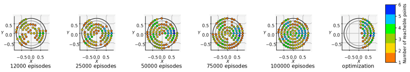
Figure 3: Top-view of the feasibility region: (1-5) for different number of episodes of the training phase (the number of reachable points is computed for each $X$,$Y$ pair) and (right) in the case of the baseline FDDP.

We used a computer with the following hardware specifications: CPU AMD Ryzen 5 3600, GPU Nvidia GTX1650 4GB, RAM 16 GB DDR4 3200 MHz. During training we generated targets inside a predefined training region. This samples are generated randomly inside a cylinder centered on the robot’s initial CoM, with a radius from 0 to $0.65$ m and a height from $0.25$ m to $0.5$ m. The size was selected to push the system to its performance limits. The parameters of the robot, controller and simulation are presented in Table I.

TABLE I: Controller, Planner, Simulator parameters

Variable	Name	Range
$m$	Robot Mass [$kg$]	1.5
P	Proportional gain	10
D	Derivative gain	0.2
$\mathbf{q}_{0}$	Nominal configuration	$\begin{bmatrix}0&-0.75&1.5\end{bmatrix}$ [$rad$]
$dT$	Simulator time step [$s$]	0.001
$\tau_{max}$	Max torque [$Nm$]	8
$f_{th}$	Touch-down force th. [$N$]	1
$N_{exp}$	Num. of expl. steps	1280 (GRL), 10e4 (E2E)
$b_{s}$	Batch size	256 (GRL), 512 (E2E)
$n_{exp}$	Expl. noise	0.4 (GRL), 0.3 (E2E)
$tg_{rep}$	Landing target repetition	5 (GRL), 20 (E2E)
$N_{train}$	Training step interval	1 (GRL), 100 (E2E)

IV-1 Nonlinear Trajectory Optimisation

The first approach to compare with is a standard optimal control strategy based on FDDP. FDDP is one of the most efficient optimisation algorithms for whole-body control [32] because it takes full advantage of the intrinsic sparse structure of the optimal control problem. The FDDP solver is implemented with the optimal control library Crocoddyl [33] and uses the library Pinocchio [34] to enable fast computations of costs, dynamics, and their derivatives.

For the problem at hand, we discretised the trajectory into $N$ successive knots with a timestep $dT=0.001$ $s$ to ensure high precision. As decision variables we chose the joint torques. We split the jump in three phases: thrusting, flying, and landed. The constraints in FDDP are encoded as soft penalties in the cost. We encoded friction cones, and tracking of foot locations and velocities at the thrusting/landed stages, respectively. We added a tracking cost for the CoM reference during the flying phase to encourage the robot to lift-off. We regularized control inputs and states throughout the horizon.

IV-2 End-to-end RL

At the opposite side of the spectrum of optimal control is the application of approaches entirely based on Deep Learning, i.e., using RL end-to-end without injecting any prior domain knowledge. The RL agent sets joint position references to a low-level (PD)+gravity compensation controller. The use of a PD controller allows the system to inherit the stabilisation properties of the feedback controller, but at the same time, it allows for explosive torques (by regulating the references to have a bigger error w.r.t. to the actual positions). We query the action until the apex moment because we need to have set-points for the joints also when the leg is air-borne. After apex, we set the default configuration $\mathbf{q}_{0}$ for the landing. To be more specific, instead of directly setting the joint references $\mathbf{q}^{d}$, the control policy produces as action $\mathbf{a}$ joint angle deviations $\mathbf{\tilde{q}}\in\mathbb{R}^{3}$ w.r.t. to the nominal joint angle configuration $\mathbf{q}_{0}$.

As suggested by [35, 36] to ease the learning, we run at a frequency that is 1/5th than the controller one (1 $kHz$). We aggregate the reward for each control loop iteration and perform a training every $N_{train}=100$ queries. We terminate the episode if: 1) a touchdown is detected, 2) the robot has fallen (i.e. the base link close to the ground), 3) we reach singularity 4) a timeout of 2.5 $s$ is reached. We include in the state CoM and joint position/velocity. Since the domain is not changing (and the state is Markovian), augmenting the state with the history of some past samples [37, 12] was not necessary, therefore we tried to keep the problem dimensionality as low as possible. Hence, the observation state becomes ($\mathbf{c}$, $\mathbf{q}$, $\mathbf{\dot{c}}$, $\mathbf{\dot{q}}$, $\mathbf{c}_{tg}$). As in the case of the GRL approach, the initial state at the start of each episode is set at the nominal joint pose ($\mathbf{c}_{0},\mathbf{q}_{0}$), with zero velocity. We also encourage smoothness by penalizing the quantity $\mathbf{\tilde{q}}^{j}-\mathbf{\tilde{q}}^{j-1}$. Because of the different units, to have better conditioning in the gradient of the NN, we scale each state variable against its range. With respect to the GRL approach we increase the batch size to 512 to collect more observations for training. We provide the feasibility rewards $C_{i}$ at each loop as differential w.r.t. the previous loop. This approach is meant to ease learning while converging to the same solution [38]. At the end of each episode, we strongly penalize the lack of a touch-down event, and use the same target function (9) to encourage landing close to the target. The fact that we provide this quantity at every step enables us to achieve an informative reward [38] also before the touchdown. Following the curriculum learning idea [39], we gradually increase the difficulty of the jump enlarging the bounds of the training region (where the targets are sampled) in accordance with the number of episodes and the average reward.

IV-A Policy performance: the feasibility region

We tested the agent in inference mode, for omni-directional jumps at different heights, for 726 target positions uniformly spaced on a grid (test region) of the same shape of the training region. The test region is 20$\%$ bigger than the training region, in order to demonstrate the generalisation abilities of the system.

The policy was periodically evaluated on the test region set in order to assess the evolution of the models stored during the training phase. To measure the quality of a jump, we used the Relative Percentual Error (RPE), which we define as the distance between the touch-down and the desired target point, divided by the jump length. The feasibility region represents the area where the agent is capable of an accurate landing, i.e. RPE $\leq 10\%$.

IV-A1 Performance baseline: Trajectory Optimisation

We compared the approach with the baseline FDDP approach repeating the same optimisation for all the points in the test region without changing the costs’weights and limiting the number of iterations to $500$. For optimal control, the average computation time was $17$ $s$ for back jumps and $7.6$ s for front jumps while a single evaluation of the NN requires only $0.7$ $ms$. Fig. 3 (right) shows that a reasonable accuracy is obtained for landing locations in the front of the robot, while FDDP behaves poorly for locations in the back of the robot. Computing the mean RPE separately for the back region and the front region, we obtained an accuracy of 52 $\%$ and 16.5$\%$, respectively.

IV-A2 Performance of the GRL approach

We repeated the simulations on the test region using the GRL approach with the default NN and with a NN where we halved the number of neurons in each hidden layer (half NN). Fig. 4 shows that, in both cases, with our GRL approach the RPE decreases (i.e. accuracy increases) monotonically with the number of episodes. In the front case, going from approximately 40$\%$ to 16$\%$ for 100k episodes. A satisfactory level (i.e. RPE 20$\%$ for front jumps) is already achieved after 50k episodes. All the feasibility constraints turn out to be mostly satisfied after 10k episodes. The figure also shows that the GRL approach always outperforms the standard optimisation method in terms of jump accuracy in the case of back jumps, achieving a comparable accuracy for front jumps.

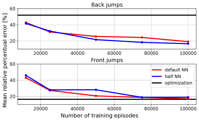
Figure 4: Plot of the average RPE as a function of the number of training episodes.

Halving the number of neurons, the two models behave with similar accuracy, showing that the RL model could ideally be further simplified. From Fig. 3 we can observe that the feasibility region expands with the number of training epochs. In the same figure we can see that the test region (black cylinder) is bigger than the region where we trained the NN (gray cylinder), demonstrating its extrapolation capabilities. It is important to remark that the GRL approach is also capable, to some extent, to learn the dynamics and compensate the tracking inaccuracies of the underlying low-level controller. This is shown in the accompanying video by the purple ball that represents the ideal landing location (i.e. if the CoM lift-off velocity associated to each action was perfectly tracked). The purple ball is different from the target location (blue ball) because of tracking inaccuracies but the agent learned to provide a lift-off velocity that compensates for these, managing to reach accurately the desired location (blue ball). In the same video we show how that the quality of the jumps steadily improves with the number of training episodes.

IV-A3 Performance baseline: end to end RL

We did not achieve satisfactory results with the E2E approach. The reward function had an erratic behaviour during the training and even after 1M of training steps there were only a few targets out of $726$ where the algorithm managed to attain an error below $10$ $\%$. More details are reported in the accompanying video.

V Conclusions

In this work we proposed a guided RL based strategy to perform omni-directional jumps on uneven terrain with a legged robot. Exploiting some domain knowledge and taking a few assumptions on the shape of the jump trajectory, we have shown that, in a few thousand episodes of training, the agent obtains the ability to jump in a big area maintaining high accuracy while reaching the boundary of his performances (deriving from the the physical limitations of the machine). The approach manages also to learn and proficiently compensate from the tracking inaccuracies of the low-level controller. The proposed approach is very efficient (it requires a small number of training episodes to reach a good performance), it achieves a good generalisation (e.g., by executing jumps in a region 20% larger than the one used for training), and it outperforms a standard end-to-end RL that resulted not able to learn the jumping motion. Compared to optimal control, the GRL approach 1) achieves the same level of performance in front jumps, but is also able to perform backward jumps (optimal control is not) 2) requires several orders of magnitude lower computation time. In the future, we plan to extend the approach to a full quadruped robot, considering not only linear but also angular motions. Leveraging the angular part we can build a framework that is able to perform a variety of jumping motions (e.g. twist, somersault, barrel jumps) on inclined surfaces. We are also seeking ways to improve robustness by including robot non idealities in the learning phase and to speed up the training phase by leveraging parallel computation.

References

- [1] F. Jenelten, R. Grandia, F. Farshidian, and M. Hutter, “Tamols: Terrain-aware motion optimization for legged systems,” IEEE Transactions on Robotics, vol. 38, no. 6, pp. 3395–3413, 2022.
- [2] F. Roscia, M. Focchi, A. D. Prete, D. G. Caldwell, and C. Semini, “Reactive landing controller for quadruped robots,” 2023.
- [3] H.-W. Park, P. M. Wensing, and S. Kim, “High-speed bounding with the mit cheetah 2: Control design and experiments,” The International Journal of Robotics Research, vol. 36, no. 2, pp. 167–192, 2017. [Online]. Available: https://doi.org/10.1177/0278364917694244
- [4] J. K. Yim, B. R. P. Singh, E. K. Wang, R. Featherstone, and R. S. Fearing, “Precision robotic leaping and landing using stance-phase balance,” IEEE Robotics and Automation Letters, vol. 5, no. 2, pp. 3422–3429, 2020.
- [5] C. Nguyen and Q. Nguyen, “Contact-timing and trajectory optimization for 3d jumping on quadruped robots,” in 2022 IEEE/RSJ International Conference on Intelligent Robots and Systems (IROS), 2022, pp. 11 994–11 999.
- [6] M. Chignoli and S. Kim, “Online trajectory optimization for dynamic aerial motions of a quadruped robot,” in 2021 IEEE International Conference on Robotics and Automation (ICRA). IEEE, 2021, pp. 7693–7699.
- [7] G. García, R. Griffin, and J. Pratt, “Time-varying model predictive control for highly dynamic motions of quadrupedal robots,” in 2021 IEEE International Conference on Robotics and Automation (ICRA), 2021, pp. 7344–7349.
- [8] M. Chignoli, S. Morozov, and S. Kim, “Rapid and reliable quadruped motion planning with omnidirectional jumping,” in 2022 International Conference on Robotics and Automation (ICRA), 2022, pp. 6621–6627.
- [9] C. Mastalli, W. Merkt, G. Xin, J. Shim, M. Mistry, I. Havoutis, and S. Vijayakumar, “Agile maneuvers in legged robots:a predictive control approach,” ArXiv, 2022.
- [10] T. P. Lillicrap, J. J. Hunt, A. Pritzel, N. M. O. Heess, T. Erez, Y. Tassa, D. Silver, and D. Wierstra, “Continuous control with deep reinforcement learning,” CoRR, vol. abs/1509.02971, 2015.
- [11] C. Gehring, S. Coros, M. Hutler, C. Dario Bellicoso, H. Heijnen, R. Diethelm, M. Bloesch, P. Fankhauser, J. Hwangbo, M. Hoepflinger, and R. Siegwart, “Practice Makes Perfect: An Optimization-Based Approach to Controlling Agile Motions for a Quadruped Robot,” IEEE Robot. Autom. Mag., vol. 23, no. 1, pp. 34–43, 2016.
- [12] J. Hwangbo, J. Lee, A. Dosovitskiy, D. Bellicoso, V. Tsounis, V. Koltun, and M. Hutter, “Learning agile and dynamic motor skills for legged robots,” Science Robotics, vol. 4, no. 26, pp. 1–20, 2019.
- [13] X. Peng, E. Coumans, T. Zhang, T.-W. Lee, J. Tan, and S. Levine, “Learning agile robotic locomotion skills by imitating animals,” Robotics: Science and Systems, 07 2020.
- [14] G. Ji, J. Mun, H. Kim, and J. Hwangbo, “Concurrent Training of a Control Policy and a State Estimator for Dynamic and Robust Legged Locomotion,” IEEE Robotics and Automation Letters, vol. 7, no. 2, pp. 4630–4637, 2022.
- [15] N. Rudin, D. Hoeller, P. Reist, and M. Hutter, “Learning to walk in minutes using massively parallel deep reinforcement learning,” in Conference on Robot Learning. PMLR, 2022, pp. 91–100.
- [16] P. Fankhauser, M. Hutter, C. Gehring, M. Bloesch, M. A. Hoepflinger, and R. Siegwart, “Reinforcement learning of single legged locomotion,” IEEE Int. Conf. Intell. Robot. Syst., pp. 188–193, 2013.
- [17] M. Bogdanovic, M. Khadiv, and L. Righetti, “Model-free reinforcement learning for robust locomotion using demonstrations from trajectory optimization,” Frontiers in Robotics and AI, vol. 9, 2022. [Online]. Available: https://www.frontiersin.org/articles/10.3389/frobt.2022.854212
- [18] G. Bellegarda, C. Nguyen, and Q. Nguyen, “Robust quadruped jumping via deep reinforcement learning,” 2023.
- [19] G. Grandesso, E. Alboni, G. P. Papini, P. M. Wensing, and A. D. Prete, “CACTO: Continuous Actor-Critic With Trajectory Optimization - Towards Global Optimality,” IEEE Robotics and Automation Letters, vol. 8, no. 6, pp. 3318–3325, 2023.
- [20] X. B. Peng and M. van de Panne, “Learning locomotion skills using deeprl: Does the choice of action space matter?” in Proc. ACM SIGGRAPH / Eurographics Symposium on Computer Animation, 2017.
- [21] G. Bellegarda and K. Byl, “Training in task space to speed up and guide reinforcement learning,” in 2019 IEEE/RSJ International Conference on Intelligent Robots and Systems (IROS), 2019, pp. 2693–2699.
- [22] S. Chen, B. Zhang, M. W. Mueller, A. Rai, and K. Sreenath, “Learning Torque Control for Quadrupedal Locomotion,” ArXiv, 2022. [Online]. Available: http://arxiv.org/abs/2203.05194
- [23] M. Aractingi, P.-A. Léziart, T. Flayols, J. Perez, T. Silander, and P. Souères, “Controlling the Solo12 Quadruped Robot with Deep Reinforcement Learning,” Aug. 2022, working paper or preprint. [Online]. Available: https://hal.laas.fr/hal-03761331
- [24] P. Henderson, J. Hu, J. Romoff, E. Brunskill, D. Jurafsky, and J. Pineau, “Towards the systematic reporting of the energy and carbon footprints of machine learning,” The Journal of Machine Learning Research, vol. 21, no. 1, pp. 10 039–10 081, 2020.
- [25] A. M. Zador, “A critique of pure learning and what artificial neural networks can learn from animal brains,” Nature communications, vol. 10, no. 1, p. 3770, 2019.
- [26] H. Shen, J. Yosinski, P. Kormushev, D. G. Caldwell, and H. Lipson, “Learning fast quadruped robot gaits with the rl power spline parameterization,” Cybernetics and Information Technologies, vol. 12, no. 3, pp. 66–75, 2013. [Online]. Available: https://doi.org/10.2478/cait-2012-0022
- [27] T. Kim and S.-H. Lee, “Quadruped locomotion on non-rigid terrain using reinforcement learning,” ArXiv, vol. abs/2107.02955, 2021. [Online]. Available: https://api.semanticscholar.org/CorpusID:235755354
- [28] Y. Ji, Z. Li, Y. Sun, X. B. Peng, S. Levine, G. Berseth, and K. Sreenath, “Hierarchical reinforcement learning for precise soccer shooting skills using a quadrupedal robot,” in 2022 IEEE/RSJ International Conference on Intelligent Robots and Systems (IROS), 2022, pp. 1479–1486.
- [29] S. Fujimoto, H. Hoof, and D. Meger, “Addressing function approximation error in actor-critic methods,” in International Conference on Machine Learning, 2018, pp. 1582–1591.
- [30] M. Grzes, Reward shaping in episodic reinforcement learning. ACM, 2017.
- [31] M. Focchi, F. Roscia, and C. Semini, “Locosim: an open-source cross-platform robotics framework,” 2023.
- [32] R. Budhiraja, J. Carpentier, C. Mastalli, and N. Mansard, “Differential Dynamic Programming for Multi-Phase Rigid Contact Dynamics,” in IEEE International Conference on Humanoid Robots, 2018.
- [33] C. Mastalli, R. Budhiraja, W. Merkt, G. Saurel, B. Hammoud, M. Naveau, J. Carpentier, L. Righetti, S. Vijayakumar, and N. Mansard, “Crocoddyl: An Efficient and Versatile Framework for Multi-Contact Optimal Control,” Proceedings - IEEE International Conference on Robotics and Automation, no. March 2020, pp. 2536–2542, 2020.
- [34] J. Carpentier, G. Saurel, G. Buondonno, J. Mirabel, F. Lamiraux, O. Stasse, and N. Mansard, “The Pinocchio C++ library – A fast and flexible implementation of rigid body dynamics algorithms and their analytical derivatives,” in IEEE International Symposium on System Integrations (SII), 2019.
- [35] S. Gangapurwala, L. Campanaro, and I. Havoutis, “Learning Low-Frequency Motion Control for Robust and Dynamic Robot Locomotion,” arXiv, 2022. [Online]. Available: http://arxiv.org/abs/2209.14887
- [36] T. Z. Zhao, V. Kumar, S. Levine, and C. Finn, “Learning Fine-Grained Bimanual Manipulation with Low-Cost Hardware,” arXiv, 2023. [Online]. Available: http://arxiv.org/abs/2304.13705
- [37] M. Aractingi, P.-A. Léziart, T. Flayols, J. Perez, T. Silander, P. Souères, and P. Soueres, “Controlling the Solo12 Quadruped Robot with Deep Reinforcement Learning,” Scientific Reports, vol. 13, 2023.
- [38] S. H. Jeon, S. Heim, C. Khazoom, and S. Kim, “Benchmarking potential based rewards for learning humanoid locomotion,” in 2023 IEEE International Conference on Robotics and Automation (ICRA), 2023, pp. 9204–9210.
- [39] Y. Bengio, J. Louradour, R. Collobert, and J. Weston, “Curriculum learning,” ACM International Conference Proceeding Series, vol. 382, no. November, 2009.