Coupled-cluster theory for trapped bosonic mixtures

Abstract

We develop a coupled-cluster theory for bosonic mixtures of binary species in external traps, providing a promising theoretical approach to demonstrate highly accurately the many-body physics of mixtures of Bose-Einstein condensates. The coupled-cluster wavefunction for the binary species is obtained when an exponential cluster operator $e^{T}$, where $T=T^{(1)}+T^{(2)}+T^{(12)}$ and $T^{(1)}$ accounts for excitations in species-1, $T^{(2)}$ for excitations in species-2, and $T^{(12)}$ for combined excitations in both species, acts on the ground state configuration prepared by accumulating all bosons in a single orbital for each species. We have explicitly derived the working equations for the bosonic mixtures by truncating the cluster operator upto the single and double excitations and using an arbitrary sets of orthonormal orbitals for each of the species. Further, the comparatively simplified version of the working equations are formulated using the Fock-like operators. Finally, using an exactly solvable many-body model for bosonic mixtures that exists in the literature allows us to implement and test the performance and accuracy of the coupled-cluster theory for situations with balanced as well as imbalanced boson numbers and for weak to moderately strong intra- and inter-species interaction strengths. The comparison between our computed results using coupled-cluster theory with the respective analytical exact results displays remarkable agreement exhibiting excellent success of the coupled-cluster theory for bosonic mixtures. All in all, the correlation exhaustive coupled-cluster theory shows encouraging results and it could be a promising approach in paving the way for high-accuracy modelling of various bosonic mixture systems.

I INTRODUCTION

Mixtures of bosonic species created from ultracold quantum gasses are highly investigated topic, providing more degrees-of-freedom compared to single species, due to the advanced controllability of the system’s parameters by the state of the art experiments. Excellent experimental control of the strengths of inter- and intra-species interactions and of the external confinement establishes mixtures of bosonic species as a rich model to investigate many-body quantum physics. A great variety of physical phenomena involving mixtures of bosonic species have attracted much attention, such as, the phase separation [1], condensate depletion [2], fermionization [3], quantum phase transition in waveguides [4], persistent currents [5], quantum mechanical stabilization [6], entanglement induced interactions [7], the miscible to immiscible phase transition [8, 9], spin-charge separation [10], emergence of spin-roton [11], ferrodark solitons [12], and quantum droplets [13].

The ground-state properties of trapped bosonic mixtures have been extensively investigated both theoretically and experimentally [14, 15, 16, 17, 18, 19, 20, 26, 21, 22, 24, 23, 25]. In terms of theoretical description, although many observations of bosonic mixtures so far have been explained by applying the standard mean-field theory, namely, Gross–Pitaevskii theory, the many-body modelling is an indispensable tool to capture fundamental understanding and outline new schemes of variety of quantum phenomena for applications. Presently, the popularly available many-body theories are the quantum Monte Carlo method [28, 27], the Bose-Hubbard model [29, 30], self-consistent many-body theory [31] for mixtures, and the most successful in accounting for quantum correlations, the multilayer multiconfigurational time-dependent Hartree method [32, 33, 34, 35].

Since the coupled-cluster theory was reformulated and introduced to electron-structure theory in [37, 36], it has become one of the most successful methods of choice in quantum chemistry when accuracy is concerned [38, 39]. For many-fermion systems, the coupled-cluster theory has already been proved to be a very reliable and accurate approach [40, 41, 42], also in the relativistic regime of interest [43, 46, 44, 45]. In Ref [47], a coupled-cluster theory for trapped interacting indistinguishable bosons was derived and a few numerical applications were shown upto $10^{4}$ particles with sufficiently strong inter-boson interaction strength. Their investigation suggests that the coupled-cluster theory would be a practical approach to apply beyond single-component bosonic systems and thereby study further the bosonic mixtures of different species. Here, we would like to mention some of the recent advancements of coupled-cluster theory, such as, for electron-phonon systems [48], polarons [49, 50], and the investigation of multiexcitonic interactions [51]

In this work we develop a theoretical framework of the coupled-cluster theory for systems of trapped binary bosonic mixtures. The general theory includes all kinds of excitations and we call it coupled-cluster theory for mixtures, or, briefly, CC-M. To begin with, we include the single and double excitations in the mixture of two species, and thereby, according to the order of excitations included the theory becomes the coupled-cluster singles doubles theory for bosonic mixtures, CCSD-M. We derive the working equations of the coupled-cluster theory with an arbitrary sets of orthonormal orbitals and also using Fock-like operators. We implement the theory and illustrate the potential usage by comparing it to an exactly solvable many-body model. This enables us to get precise results on how accurate we are in scenarios that occur for binary mixtures with balanced and imbalanced particle numbers and having weak to strong intra- and inter-species interaction strengths.

The structure of the paper is as follows: In section II, we present the CC-M ansatz and provide the basic formulation of the cluster operators for the excitations for the mixture. Section III presents the details of Fock-like operators for the bosonic mixture of binary species. In Section IV, the coupled-cluster theory for the bosonic mixtures is developed and the detailed derivation is shown. In Section V, we provide the potential of our coupled-cluster theory by comparing the results for scenarios when the mixtures have balanced and imbalanced particle numbers and for different strengths of intra- and inter-species interaction to the analytical results from an exactly solvable model. Finally, in Section VI, we summarize and conclude our work. The appendices provide additional details on the derivation of the theory and its implementation.

II Theoretical framework for coupled-cluster theory for bosonic mixtures

In order to develop the coupled-cluster theory for binary mixture of bosons, we consider the number of bosons in species-1 and species-2 to be $N_{1}$ and $N_{2}$, respectively, with the total number of bosons $N=N_{1}+N_{2}$. For simplicity, we consider the bosons to be spinless. We introduce the number of one-particle functions or orbitals for species-1 as $M_{1}$ and for species-2 as $M_{2}$. We start from the Schrödinger equation, $H|\Psi\rangle=E_{0}|\Psi\rangle$, where $E_{0}$ is the exact energy and $\Psi$ is the coupled-cluster wavefunction, to be defined below. The Hamiltonian $H$ for the mixture of two species can be written as

$${H}={H}^{(1)}+{H}^{(2)}+{H}^{(12)},$$

$${H}^{(1)}=\sum_{p,q}h_{\bar{p}\bar{q}}^{(1)}{a}_{p}^{\dagger}{a}_{q}+\dfrac{1}{2}\sum_{p,q,r,s}V_{\bar{p}\bar{q}\bar{r}\bar{s}}^{(1)}{a}_{p}^{\dagger}{a}_{q}^{\dagger}{a}_{r}{a}_{s},$$

$${H}^{(2)}=\sum_{i,j}h_{ij}^{(2)}{b}_{i}^{\dagger}{b}_{j}+\dfrac{1}{2}\sum_{i,j,k,l}V_{ijkl}^{(2)}{b}_{i}^{\dagger}{b}_{j}^{\dagger}{b}_{k}{b}_{l},$$

$${H}^{(12)}=\sum_{p,q,i,j}V_{\bar{p}i\bar{q}j}^{(12)}{a}_{p}^{\dagger}{b}_{i}^{\dagger}{a}_{q}{b}_{j}.$$ (1)

Here, ${a}_{p}^{\dagger}$ and ${a}_{p}$, where $p=1,2,...,M_{1}$, are the bosonic creation and destruction operators, respectively, corresponding to the orbitals $\varphi_{p}(\textbf{r}_{1})$ of species-1 and similarly for species-2, the corresponding operators are ${b}_{i}^{\dagger}$ and ${b}_{i}$, where $i=1,2,...,M_{2}$, for the orbitals $\psi_{i}(\textbf{r}_{2})$. The symbols $\{pqrs\}$ and $\{ijkl\}$ are used for the species-1 and species-2, respectively, until specified differently. Furthermore, to ease the reading of equations, whenever we have indices in matrix elements for species-1, we write a bar on top. For instance in ${H}^{(12)}$, the matrix element is $V_{\bar{p}i\bar{q}j}^{(12)}$ where the variables are $p$ and $q$ for species-1. The creation and destruction operators follow the usual bosonic commutator relations which read

$$[{a}_{p},{a}_{q}^{\dagger}]=\delta_{pq},[{a}_{p},{a}_{q}]=0,[{a}_{p}^{\dagger},{a}_{q}^{\dagger}]=0,$$

$$[{b}_{i},{b}_{j}^{\dagger}]=\delta_{ij},[{b}_{i},{b}_{j}]=0,[{b}_{i}^{\dagger},{b}_{j}^{\dagger}]=0,$$

$$[{a}_{p},{b}_{i}^{\dagger}]=0,[{a}_{p},{b}_{i}]=0,[{a}_{p}^{\dagger},{b}_{i}^{\dagger}]=0.$$ (2)

In the Hamiltonian Eq. II, the one-particle operators for species-1 and species-2 are

$$h_{\bar{p}\bar{q}}^{(1)}=\int\varphi_{p}^{*}\hat{h}^{(1)}\varphi_{q}d\textbf{r}_{1},$$

$$h_{ij}^{(2)}=\int\psi_{i}^{*}\hat{h}^{(2)}\psi_{j}d\textbf{r}_{2},$$ (3)

respectively, and the two-particle interactions in the Hamiltonian Eq. II are given by

$$V_{\bar{p}\bar{q}\bar{r}\bar{s}}^{(1)}=\int\int\varphi_{p}^{*}\varphi_{q}^{*}{V}^{(1)}(\textbf{r}_{1}-\textbf{r}_{1}^{\prime})\varphi_{r}\varphi_{s}d\textbf{r}_{1}d\textbf{r}_{1}^{\prime},$$

$$V_{ijkl}^{(2)}=\int\int\psi_{i}^{*}\psi_{j}^{*}{V}^{(2)}(\textbf{r}_{2}-\textbf{r}_{2}^{\prime})\psi_{k}\psi_{l}d\textbf{r}_{2}d\textbf{r}_{2}^{\prime},$$

$$V_{\bar{p}i\bar{q}j}^{(12)}=\int\int\varphi_{p}^{*}\psi_{i}^{*}{V}^{(12)}(\textbf{r}_{1}-\textbf{r}_{2})\varphi_{q}\psi_{j}d\textbf{r}_{1}d\textbf{r}_{2}.$$ (4)

Here the first and second terms stand for the two-particle interactions for species-1 and species-2, respectively. The last term indicates the two-particle interaction between the bosons of species-1 and species-2.

In order to solve the Schrödinger equation $H|\Psi\rangle=E_{0}|\Psi\rangle$ with the Hamiltonian presented in Eq. II, using the coupled-cluster theory, we start with the definition of the exact wavefunction of bosonic mixture which is obtained by employing an exponential operator onto the ground configuration

$$|\Psi\rangle=e^{T}|\phi_{0}\rangle.$$ (5)

The ground configuration takes the form of product state, $\phi_{0}=\prod_{n=1}^{N_{1}}\varphi_{1}(r_{1n})\prod_{m=1}^{N_{2}}\psi_{1}(r_{2m})$, which defines the standard mean-field for the bosonic mixture, also see below. We note that other mean-fields are possible for bosons [52, 53], but we will not pursue such a choice here.

For the bosonic mixture, the cluster operator $T$ is conveniently divided into three parts,

$$T=T^{(1)}+T^{(2)}+T^{(12)}.$$ (6)

Here, the cluster operators, $T^{(1)}$, $T^{(2)}$, and $T^{(12)}$ correspond the superposition of excitation operators. Moreover, $T^{(1)}$ are identical to the single-component cluster operator and operates only on the Hilbert space of species-1. The same holds true for $T^{(2)}$, but it operates only on the Hilbert space of species-2. In contrast, $T^{(12)}$ yields the simultaneous excitations in the Hilbert spaces of both species-1 and species-2. In terms of excitations, the cluster operators can be written as

$$T^{(1)}=\sum_{n=1}^{N_{1}}T_{n}^{(1)}=\sum_{n=1}^{N_{1}}t_{n}^{(1)}(a_{1})^{n}=\sum_{n=1}^{N_{1}}\sum_{p_{1},...,p_{n}=2}^{M_{1}}c_{p_{1}p_{2}...p_{n}}a_{p_{1}}^{\dagger}a_{p_{2}}^{\dagger}...a_{p_{n}}^{\dagger}(a_{1})^{n},$$ (7)

$$T^{(2)}=\sum_{m=1}^{N_{2}}T_{m}^{(2)}=\sum_{m=1}^{N_{2}}t_{m}^{(2)}(b_{1})^{m}=\sum_{m=1}^{N_{2}}\sum_{i_{1},...,i_{m}=2}^{M_{2}}d_{i_{1}i_{2}...i_{m}}b_{i_{1}}^{\dagger}b_{i_{2}}^{\dagger}...b_{i_{m}}^{\dagger}(b_{1})^{m}.$$ (8)

Note that for each species the first orbital is occupied and the second orbital and onward are the virtual orbitals. In Eq. 7, $t_{n}^{(1)}=\sum_{p_{1},...,p_{n}=2}^{M_{1}}c_{p_{1}p_{2}...p_{n}}a_{p_{1}}^{\dagger}a_{p_{2}}^{\dagger}...a_{p_{n}}^{\dagger}$ creates the excitations in the virtual orbitals of species-1. Similarly, in Eq. 8, $t_{m}^{(2)}=\sum_{i_{1},...,i_{m}=2}^{M_{2}}d_{i_{1}i_{2}...i_{m}}b_{i_{1}}^{\dagger}b_{i_{2}}^{\dagger}...b_{i_{m}}^{\dagger}$ generates the excitations in the virtual orbitals of species-2. $T^{(12)}$ has the form

$$T^{(12)} = \sum_{n^{\prime}=1}^{N_{1}}\sum_{m^{\prime}=1}^{N_{2}}T_{n^{\prime}m^{\prime}}^{(12)}=\sum_{n^{\prime}=1}^{N_{1}}\sum_{m^{\prime}=1}^{N_{2}}t_{n^{\prime}m^{\prime}}^{(12)}(a_{{1}})^{n^{\prime}}(b_{1})^{m^{\prime}}$$ (9)

$$= \sum_{n^{\prime}=1}^{N_{1}}\sum_{m^{\prime}=1}^{N_{2}}\sum_{p_{1},...,p_{n^{\prime}}=2}^{M_{1}}\sum_{i_{1},...,i_{m^{\prime}}=2}^{M_{2}}e_{p_{1}...p_{n^{\prime}}i_{1}...i_{m^{\prime}}}a_{p_{1}}^{\dagger}...a_{p_{n^{\prime}}}^{\dagger}b_{i_{1}}^{\dagger}b_{i_{2}}^{\dagger}...b_{i_{m^{\prime}}}^{\dagger}(a_{{1}})^{n^{\prime}}(b_{1})^{m^{\prime}}.$$

In the expression of $T^{(12)}$, one can find that $t_{n^{\prime}m^{\prime}}^{(12)}=\sum_{p_{1},...,p_{n^{\prime}}=2}^{M_{1}}\sum_{i_{1},...,i_{m^{\prime}}=2}^{M_{2}}e_{p_{1}...p_{n^{\prime}}i_{1}...i_{m^{\prime}}}a_{p_{1}}^{\dagger}...a_{p_{n^{\prime}}}^{\dagger}\\ b_{i_{1}}^{\dagger}b_{i_{2}}^{\dagger}...b_{i_{m^{\prime}}}^{\dagger}$ is responsible for the simultaneous excitations in both species. In Eqs. 7 and  8, the expansions of $T^{(1)}=T_{1}^{(1)}+T_{2}^{(1)}+T_{3}^{(1)}+...$ and $T^{(2)}=T_{1}^{(2)}+T_{2}^{(2)}+T_{3}^{(2)}+...$ include the singles, doubles, triples, … and so on excitations. While for $T^{(12)}=T_{11}^{(12)}+T_{12}^{(12)}+T_{21}^{(12)}+...$, see Eq. 9, the excitations start from doubles, each for one species. We shall find out the unknown coefficients $c_{p_{1}p_{2}...p_{n}}$, $d_{i_{1}i_{2}...i_{m}}$, and $e_{p_{1}...p_{n^{\prime}}i_{1}...i_{m^{\prime}}}$ when we will explicitly develop below the coupled-cluster theory for bosonic mixtures. Since the summations in Eqs. 7 to  9 are unrestricted, the coefficients do not depend on the ordering of the subscripts. Also, it is convenient to find the commutation relations among the cluster operators, $[T_{n}^{(1)},T_{n^{\prime}}^{(1)}]=[T_{m}^{(2)},T_{m^{\prime}}^{(2)}]=[T_{n}^{(1)},T_{m}^{(2)}]=[T_{n}^{(1)},T_{n^{\prime}m^{\prime}}^{(12)}]=[T_{m^{\prime}}^{(2)},T_{n^{\prime}m^{\prime}}^{(12)}]=[T_{nm}^{(12)},T_{n^{\prime}m^{\prime}}^{(12)}]=0$. The implication of the commutation relations among the cluster operators is that the excitation operator is breakable to a product of all the partial excitation operators, i.e., $e^{T}|\phi_{0}\rangle=e^{T_{1}}e^{T_{2}}e^{T_{12}}|\phi_{0}\rangle$. Note that, as $T$ is the excitation operator, the wavefunction in Eq. 5 satisfies the intermediate normalization $\langle\phi_{0}|\Psi\rangle=1$.

III Fock-like operators for a bosonic mixture of binary species

For the study of the coupled-cluster theory for bosonic mixtures, we will first derive the working equations when the orbitals are arbitrary or unspecified to demonstrate a general perspective of the theory. However, we will also utilize the orbitals arising from the Fock-like operators to give an illustrative example. To derive the Fock-like operators, we start from the mean-field energy functional for a mixture which reads

$$E_{\text{MF}} = N_{1}\Bigg{[}\int d\textbf{r}_{1}\varphi_{1}^{*}(\textbf{r}_{1})\Big{(}{h}^{(1)}+\dfrac{\Lambda_{1}}{2}{J}_{11}+\dfrac{\Lambda_{21}}{2}{{J}_{21}}\Big{)}\varphi_{1}(\textbf{r}_{1})\Bigg{]}$$ (10)

$$+ N_{2}\Bigg{[}\int d\textbf{r}_{2}\psi_{1}^{*}(\textbf{r}_{2})\Big{(}{h}^{(2)}+\dfrac{\Lambda_{2}}{2}{J}_{22}+\dfrac{\Lambda_{12}}{2}{{J}_{12}}\Big{)}\psi_{1}(\textbf{r}_{2})\Bigg{]},$$

where the interaction parameters are given by $\Lambda_{1}=\lambda_{1}(N_{1}-1)$, $\Lambda_{2}=\lambda_{2}(N_{2}-1)$, $\Lambda_{21}=\lambda_{12}N_{2}$, and $\Lambda_{12}=\lambda_{12}N_{1}$, and satisfy $N_{1}\Lambda_{21}=N_{2}\Lambda_{12}$. Here $\lambda_{1}$ and $\lambda_{2}$ are the intra-species interaction strengths of species-1 and species-2, respectively, and $\lambda_{12}$ is the inter-species interaction strength between species-1 and species-2. Also, the direct interaction operators ${J}_{11}$, ${J}_{22}$, ${J}_{12}$, and ${J}_{21}$ are local operators and are defined by

$${J}_{11}=\int\varphi_{1}^{*}(\textbf{r}_{1}^{\prime}){V}^{(1)}(\textbf{r}_{1}-\textbf{r}_{1}^{\prime})\varphi_{1}(\textbf{r}_{1}^{\prime})d\textbf{r}_{1}^{\prime},$$

$${J}_{22}=\int\psi_{1}^{*}(\textbf{r}_{2}^{\prime}){V}^{(2)}(\textbf{r}_{2}-\textbf{r}_{2}^{\prime})\psi_{1}(\textbf{r}_{2}^{\prime})d\textbf{r}_{2}^{\prime},$$

$${J}_{21}=\int\psi_{1}^{*}(\textbf{r}_{2}){V}^{(12)}(\textbf{r}_{1}-\textbf{r}_{2})\psi_{1}(\textbf{r}_{2})d\textbf{r}_{2},$$

$${J}_{12}=\int\varphi_{1}^{*}(\textbf{r}_{1}){V}^{(12)}(\textbf{r}_{1}-\textbf{r}_{2})\varphi_{1}(\textbf{r}_{1})d\textbf{r}_{1}.$$ (11)

Minimizing the mean-field energy functional with respect to the orbitals $\varphi_{1}(\textbf{r}_{1})$ and $\psi_{1}(\textbf{r}_{2})$, the two-coupled mean-field equations of the mixture are derived,

$$[{h}^{(1)}+\Lambda_{1}{J}_{11}+\Lambda_{21}{J}_{21}]\varphi_{1}(\textbf{r}_{1})=\mu_{1}^{(1)}\varphi_{1}(\textbf{r}_{1}),$$

$$[{h}^{(2)}+\Lambda_{2}{J}_{22}+\Lambda_{12}{J}_{12}]\psi_{1}(\textbf{r}_{2})=\mu_{1}^{(2)}\psi_{1}(\textbf{r}_{2})$$ (12)

Here $\mu_{1}^{(1)}$ and $\mu_{1}^{(2)}$ are the chemical potentials of the ground state of species-1 and species-2, respectively. Eq. III presents the Hermitian Fock-like operators

$${F}_{1}={h}^{(1)}+\Lambda_{1}{J}_{11}+\Lambda_{21}{J}_{21},$$

$${F}_{2}={h}^{(2)}+\Lambda_{2}{J}_{22}+\Lambda_{12}{J}_{12}.$$ (13)

Eq. III determines the ground state of the bosonic mixtures and the ground state orbitals define the Fock-like operators. Now, the eigenfunctions of the Fock-like operators gives us the complete orthonormal basis sets

$${F}_{1}\varphi_{i}=\mu_{i}^{(1)}\varphi_{i},$$

$${F}_{2}\psi_{i}=\mu_{i}^{(2)}\psi_{i}.$$ (14)

From Eq. III, the eigenvalues are computed as $\langle\varphi_{i}|{F}_{1}|\varphi_{i}\rangle=\mu_{i}^{(1)}$ and $\langle\psi_{i}|{F}_{2}|\psi_{i}\rangle=\mu_{i}^{(2)}$. Using the Fock-like operators, one can simplify the general working equations by utilizing the relations between the one-body and two-body matrix elements, see details in Appendix A.

IV DERIVATION OF THE WORKING EQUATIONS

Starting from the Schrödinger equation $H|\Psi\rangle=E_{0}|\Psi\rangle$, where $H$ is given in Eq. II, and plugging the coupled-cluster ansatz Eq. 5 on both the left and right hand sides, the exact energy of the ground state can be expressed as an expectation value,

$$E_{0}=\langle\phi_{0}|e^{-T}He^{T}|\phi_{0}\rangle.$$ (15)

The transformed Hamiltonian entering the expression for the energy Eq. 15 can be expanded using the relation $\dot{A}=e^{-T}Ae^{T}=A+\dfrac{1}{1!}[A,T]+\dfrac{1}{2!}[[A,T],T]+...$. Now we break the transformed Hamiltonian in accordance with the number of operators depending on the occupied orbitals $\varphi_{1}$ and $\psi_{1}$. Here, the transformed one-particle operator is found to be

$$\dot{H_{0}} = h_{\bar{1}\bar{1}}^{(1)}\dot{a}_{1}^{\dagger}\dot{a}_{1}+\sum_{s=2}^{M_{1}}h_{\bar{1}\bar{s}}^{(1)}\dot{a}_{1}^{\dagger}\dot{a}_{s}+\sum_{s=2}^{M_{1}}h_{\bar{s}\bar{1}}^{(1)}\dot{a}_{s}^{\dagger}\dot{a}_{1}+\sum_{r,s=2}^{M_{1}}h_{\bar{r}\bar{s}}^{(1)}\dot{a}_{r}^{\dagger}\dot{a}_{s}$$ (16)

$$+ h_{11}^{(2)}\dot{b}_{1}^{\dagger}\dot{b}_{1}+\sum_{l=2}^{M_{2}}h_{1l}^{(2)}\dot{b}_{1}^{\dagger}\dot{b}_{l}+\sum_{l=2}^{M_{2}}h_{l1}^{(2)}\dot{b}_{l}^{\dagger}\dot{b}_{1}+\sum_{k,l=2}^{M_{2}}h_{kl}^{(2)}\dot{b}_{k}^{\dagger}\dot{b}_{l},$$

which includes a total of eight terms for two species, and among them the second and the sixth terms are the most intricate in evaluating the exact energy. The transformed two-body operator of the Hamiltonian is divided into three parts, $\dot{V}^{(1)}$, $\dot{V}^{(2)}$, and $\dot{V}^{(12)}$. The first, $\dot{V}^{(1)}$, and the second, $\dot{V}^{(2)}$, parts correspond to excitations in species-1 and species-2, respectively, and consist of nine terms each. The third part $\dot{V}^{(12)}$ is the most involved one as it contains the excitations in both species and it has sixteen terms. All terms are explicitly shown in Appendix C. As shown in Eqs. 16, C. Transformed two-body operators, C. Transformed two-body operators, and C. Transformed two-body operators, the transformed Hamiltonian contains transformed creation and destruction operators corresponding to the occupied and unoccupied orbitals. Now, in the following subsection, we present the expansions of the transformed creation and destruction operators.

IV.1 General relations

In this section, we derive and discuss the working equations of the coupled-cluster theory for the bosonic mixture. At first, we transform the bosonic destruction and creation operators for both the species using the expansion $\dot{A}\equiv e^{-T}Ae^{T}$. The similarity transformations of the destruction and creation operators are needed eventually to construct the transformed Hamiltonian under investigation. One can readily find, for both species, that the destruction operator corresponding to the occupied orbitals, $\varphi_{1}$ and $\psi_{1}$, and the creation operators of the virtual orbitals, $\varphi_{p}$ and $\psi_{i}$ where $p\geq 2$ and $i\geq 2$, are invariant to the coupled-cluster transformation:

$$\dot{a}_{{1}}=a_{{1}},$$

$$\dot{a}_{{p}}^{\dagger}=a_{{p}}^{\dagger},\hskip 5.69046ptp=2,3,...,M_{1},$$

$$\dot{b}_{1}=b_{1},$$

$$\dot{b}_{i}^{\dagger}=b_{i}^{\dagger},\hskip 5.69046pti=2,3,...,M_{2}.$$ (17)

In contrast, the creation operators corresponding to the orbitals occupied in $\phi_{0}$ for each species, and the destruction operators of the virtual orbitals are modified due to the similarity transformation for both species and one can readily find the relations

$$\dot{a}_{{1}}^{\dagger}=a_{{1}}^{\dagger}-\mathcal{K}_{{1}},$$

$$\dot{a}_{p}=a_{p}+\mathcal{K}_{p},$$

$$\dot{b}_{1}^{\dagger}=b_{1}^{\dagger}-\mathcal{L}_{1},$$

$$\dot{b}_{i}=b_{i}+\mathcal{L}_{i},$$ (18)

where $\mathcal{K}_{{1}}$ and $\mathcal{K}_{{p}}$ can be expressed as

$$\mathcal{K}_{{1}}=\sum_{n=1}^{N_{1}}nt_{n}^{(1)}{(a_{{1}})}^{n-1}+\sum_{n=1}^{N_{1}}\sum_{m=1}^{N_{2}}nt_{nm}^{(12)}{(a_{{1}})}^{n-1}b_{1}^{m},$$ (19)

$$\mathcal{K}_{{p}}=\sum_{n=1}^{N_{1}}nt_{n}^{(1)(p)}{(a_{{1}})}^{n}+\sum_{n=1}^{N_{1}}\sum_{m=1}^{N_{2}}n\eta_{nm}^{(12)(p)}{a_{{1}}}^{n}b_{1}^{m}.$$ (20)

Here, the operators $t_{n}^{(1)}$ and $t_{nm}^{(12)}$ are defined before, see Eqs. 7 and  9. The operators $t_{n}^{(1)(p)}$ operate in the virtual space of species-1 and create excitations, while $\eta_{nm}^{(12)(p)}$ are also responsible for excitations but acting in the virtual space of both species. $t_{n}^{(1)(p)}$ and $\eta_{nm}^{(12)(p)}$ read

$$t_{n}^{(1)(p)}=\sum_{p_{2},p_{3},...,p_{n}=2}^{M_{1}}c_{pp_{2}...p_{n}}a_{p_{2}}^{\dagger}a_{p_{3}}^{\dagger}...a_{p_{n}}^{\dagger},$$ (21)

$$\eta_{nm}^{(12)(p)}=\sum_{p_{2},p_{3},...,p_{n}=2}^{M_{1}}\sum_{i_{1},i_{2},...,i_{m}=2}^{M_{2}}e_{pp_{2}...p_{n}i_{1}i_{2}...i_{m}}a_{p_{2}}^{\dagger}a_{p_{3}}^{\dagger}...a_{p_{n}}^{\dagger}b_{i_{1}}^{\dagger}b_{i_{2}}^{\dagger}...b_{i_{m}}^{\dagger}.$$ (22)

Similarly, for species-2, $\mathcal{L}_{1}$ and $\mathcal{L}_{i}$ are expressed as

$$\mathcal{L}_{1}=\sum_{m=1}^{N_{2}}mt_{m}^{(2)}{(b_{1})}^{m-1}+\sum_{n=1}^{N_{1}}\sum_{m=1}^{N_{2}}mt_{nm}^{(12)}a_{1}^{n}b_{1}^{m-1},$$ (23)

$$\mathcal{L}_{i}=\sum_{m=1}^{N_{2}}mt_{m}^{(2)(i)}{(b_{1})}^{m}+\sum_{n=1}^{N_{1}}\sum_{m=1}^{N_{2}}m\tau_{nm}^{(12)(i)}a_{1}^{n}b_{1}^{m}.$$ (24)

The operators $t_{m}^{(2)(i)}$ generate excitations and operate in the virtual space of species-2 but the operators $\tau_{nm}^{(12)(i)}$ excite bosons in both species simultaneously. $t_{m}^{(2)(i)}$ and $\tau_{nm}^{(12)(i)}$ can be represented as

$$t_{m}^{(2)(i)}=\sum_{i_{2},i_{3},...,i_{m}=2}^{M_{2}}d_{ii_{2}...i_{m}}b_{i_{2}}^{\dagger}b_{i_{3}}^{\dagger}...b_{i_{m}}^{\dagger},$$ (25)

$$\tau_{nm}^{(12)(i)}=\sum_{p_{1},p_{2},...,p_{n}=2}^{M_{1}}\sum_{i_{2},i_{3},...,i_{m}=2}^{M_{2}}e_{p_{1}p_{2}...p_{n}ii_{2}...i_{m}}a_{p_{1}}^{\dagger}a_{p_{2}}^{\dagger}...a_{p_{n}}^{\dagger}b_{i_{2}}^{\dagger}b_{i_{3}}^{\dagger}...b_{i_{m}}^{\dagger},$$ (26)

To determine the unknown coefficients, $c_{p_{1}p_{2}...p_{n}}$, $d_{i_{1}i_{2}...i_{m}}$, and $e_{p_{1}...p_{n^{\prime}}i_{1}...i_{m^{\prime}}}$, it is recommended to expand the first few terms of $\mathcal{K}_{{1}}$, $\mathcal{K}_{{p}}$, $\mathcal{L}_{1}$, and $\mathcal{L}_{i}$. The expansions of $\mathcal{K}_{{1}}$, $\mathcal{K}_{{p}}$, $\mathcal{L}_{1}$, and $\mathcal{L}_{i}$, which are defined in Eqs. IV.1, are explicitly presented in Appendix B.

In the following calculations, it is noted that the operators $\mathcal{K}$ and $\mathcal{L}$ fulfil the commutation relation $[\mathcal{K}_{{p}},\mathcal{K}_{{q}}]=[\mathcal{K}_{{1}},\mathcal{K}_{{p}}]=0$, $[\mathcal{L}_{i},\mathcal{L}_{j}]=[\mathcal{L}_{1},\mathcal{L}_{j}]=0$, and $[\mathcal{L}_{1},\mathcal{K}_{{p}}]=[\mathcal{K}_{{1}},\mathcal{L}_{j}]=[\mathcal{L}_{i},\mathcal{K}_{{p}}]=0$. Also, the actions of the $\mathcal{K}$ and $\mathcal{L}$ on $\langle\phi_{0}|$ from the right are $\langle\phi_{0}|\mathcal{K}_{{1}}=0,\langle\phi_{0}|(a_{{1}})^{n}\mathcal{K}_{{1}}=0,\langle\phi_{0}|\mathcal{K}_{{i}}=c_{{i}}\langle\phi_{0}|a_{{1}}$ and $\langle\phi_{0}|\mathcal{L}_{1}=0,\langle\phi_{0}|(b_{1})^{m}\mathcal{L}_{1}=0,\langle\phi_{0}|\mathcal{L}_{j}=d_{j}\langle\phi_{0}|b_{1}$.

IV.2 The energy and its structure

We now calculate the energy using $E_{0}=\langle\phi_{0}|\dot{H}|\phi_{0}\rangle$. We find that the energy is given by the combination of three parts

$$E_{0}=E_{1}+E_{2}+E_{12},$$ (27)

where after some intricate algebra, one can readily find $E_{1}$, $E_{2}$, and $E_{12}$ as

$$E_{1} = N_{1}\left[h_{\bar{1}\bar{1}}^{(1)}+\dfrac{N_{1}-1}{2}V_{\bar{1}\bar{1}\bar{1}\bar{1}}^{(1)}\right]$$ (28)

$$+ N_{1}\Biggl{[}\sum_{s=2}^{M_{1}}[h_{\bar{1}\bar{s}}^{(1)}+(N_{1}-1)V_{\bar{1}\bar{1}\bar{1}\bar{s}}^{(1)}]c_{s}+\dfrac{N_{1}-1}{2}\sum_{r,s=2}^{M_{1}}V_{\bar{1}\bar{1}\bar{r}\bar{s}}^{(1)}(2c_{rs}+c_{r}c_{s})\Biggr{]},$$

$$E_{2} = N_{2}\left[h_{11}^{(2)}+\dfrac{N_{2}-1}{2}V_{1111}^{(2)}\right]$$ (29)

$$+ N_{2}\Biggl{[}\sum_{l=2}^{M_{2}}[h_{1l}^{(2)}+(N_{2}-1)V_{111l}^{(2)}]d_{l}+\dfrac{N_{2}-1}{2}\sum_{k,l=2}^{M_{2}}V_{11kl}^{(2)}(2d_{kl}+d_{k}d_{l})\Biggr{]},$$

$$E_{12}=N_{1}N_{2}\Biggl{[}V_{\bar{1}1\bar{1}1}^{(12)}+\sum_{s=2}^{M_{1}}V_{\bar{1}1\bar{s}1}^{(12)}c_{s}+\sum_{l=2}^{M_{2}}V_{\bar{1}1\bar{1}l}^{(12)}d_{l}+\sum_{s=2}^{M_{1}}\sum_{l=2}^{M_{2}}V_{\bar{1}1\bar{s}l}^{(12)}(c_{s}d_{l}+e_{ls})\Biggr{]}.$$ (30)

We notice that, in order to calculate $E_{1}$, the first and second terms of $\dot{H}_{0}$ and the first, second, and fourth terms of $\dot{V}^{(1)}$ contribute. While for $E_{2}$, the fifth and sixth terms of $\dot{H}_{0}$ and the first, second, and fourth terms of $\dot{V}^{(2)}$ contribute. To determine $E_{12}$, only the first, second, third, and sixth terms of $\dot{V}^{(12)}$ contribute, also see Appendix C.

Here, $E_{1}$ depends on the singles and doubles coefficients of species-1 and, analogously, $E_{2}$ depends on the singles and doubles coefficients of species-2. $E_{1}$ and $E_{2}$ have the analog form of single species coupled-cluster theory, whereas $E_{12}$ does not have an analog in single species theory as it is generated due to the inter-species interaction. If there is no inter-species interaction, $E_{0}$ boils down to the energy of two independent single species bosonic system. Note that the equation of $E_{0}$ presented here, Eqs. 27 to  30, is valid for all orders of coupled-cluster theory for bosonic mixtures, CC-M.

The mean-field energy, $E_{\text{MF}}=\langle\phi_{0}|{H}|\phi_{0}\rangle$, is contained in the first and fifth terms of $\dot{H}_{0}$ and the first terms of $\dot{V}^{(1)}$, $\dot{V}^{(2)}$, and $\dot{V}^{(12)}$. $E_{\text{MF}}$ is found to be

$$E_{\text{MF}}=N_{1}\left[h_{\bar{1}\bar{1}}^{(1)}+\dfrac{N_{1}-1}{2}V_{\bar{1}\bar{1}\bar{1}\bar{1}}^{(1)}\right]+N_{2}\left[h_{11}^{(2)}+\dfrac{N_{2}-1}{2}V_{1111}^{(2)}\right]+N_{1}N_{2}V_{\bar{1}1\bar{1}1}^{(12)}.$$ (31)

The definition of the correlation energy of the ground state is the difference between many-body and mean-field energies. For the binary bosonic mixtures, the correlation energy is $(E_{1}+E_{2}+E_{12})-E_{\text{MF}}$ which can be explicitly written as

$$E_{\text{cor}} = N_{1}\Biggl{[}\sum_{s=2}^{M_{1}}[h_{\bar{1}\bar{s}}^{(1)}+(N_{1}-1)V_{\bar{1}\bar{1}\bar{1}\bar{s}}^{(1)}]c_{s}+\dfrac{N_{1}-1}{2}\sum_{r,s=2}^{M_{1}}V_{\bar{1}\bar{1}\bar{r}\bar{s}}^{(1)}(2c_{rs}+c_{r}c_{s})\Biggr{]}$$ (32)

$$+ N_{2}\Biggl{[}\sum_{l=2}^{M_{2}}[h_{1l}^{(2)}+(N_{2}-1)V_{111l}^{(2)}]d_{l}+\dfrac{N_{2}-1}{2}\sum_{k,l=2}^{M_{2}}V_{11kl}^{(2)}(2d_{kl}+d_{k}d_{l})\Biggr{]}$$

$$+ N_{1}N_{2}\Biggl{[}\sum_{s=2}^{M_{1}}V_{\bar{1}1\bar{s}1}^{(12)}c_{s}+\sum_{l=2}^{M_{2}}V_{\bar{1}1\bar{1}l}^{(12)}d_{l}+\sum_{s=2}^{M_{1}}\sum_{l=2}^{M_{2}}V_{\bar{1}1\bar{s}l}^{(12)}(c_{s}d_{l}+e_{ls})\Biggr{]}.$$

In the calculation of $E_{\text{cor}}$, we have used arbitrary sets of orthonormal orbitals. If one would make use of the orbitals generating from the Fock-like operators ${F}_{1}$ and ${F}_{2}$, see Eqs. III and  III discussed in last section, and Eq. A. Relations between one-body and two-body terms in Appendix A, the correlation energy simplifies and reads

$$E_{\text{cor}} = \dfrac{N_{1}(N_{1}-1)}{2}\sum_{r,s=2}^{M_{1}}V_{\bar{1}\bar{1}\bar{r}\bar{s}}^{(1)}(2c_{rs}+c_{r}c_{s})+\dfrac{N_{2}(N_{2}-1)}{2}\sum_{k,l=2}^{M_{2}}V_{11kl}^{(2)}(2d_{kl}+d_{k}d_{l})$$ (33)

$$+N_{1}N_{2}\sum_{s=2}^{M_{1}}\sum_{l=2}^{M_{2}}V_{\bar{1}1\bar{s}l}^{(12)}(c_{s}d_{l}+e_{ls}).$$

The other terms disappear due to the facts that $\langle\varphi_{s}|{F}_{1}|\varphi_{1}\rangle=0$ and $\langle\psi_{l}|{F}_{2}|\psi_{1}\rangle=0$. All in all, the total energy of the mixture is modified to

$$E_{0}=E_{\text{MF}}-E_{\text{cor}},$$ (34)

where $E_{\text{cor}}$ is the correlation energy for the binary mixture of bosons and presented in Eq. 33.

IV.3 Equations for the coefficients

The correlation energy due to the state dressed from $\phi_{0}$ to $\Psi$ is expressed in terms of coefficients $\{c_{s}\}$, $\{d_{l}\}$, $\{c_{rs}\}$, $\{d_{kl}\}$, and $\{e_{ls}\}$. The orbitals $\phi_{i}$ and $\psi_{j}$ can be conveniently chosen to simplify $E_{\text{cor}}$, details are in the next section. Note that even the simplified form of the equations can not be utilized to determine the unknown coefficients mentioned above since $E_{0}=\langle\phi_{0}|e^{-T}He^{T}|\phi_{0}\rangle$ is not subject to a variational principle. Therefore, one requires approximations. For the coupled-cluster theory for bosonic mixtures we may chose approximations such as the combination of keeping $M_{1}$ and $M_{2}$ small and truncating the coupled-cluster excitations. In the process of truncating the excitations, one may consider $\phi_{0}$ and all the singly and doubly excited configurations analogous by the atomic structure calculations.

Here, we observe that $E_{0}|\phi_{0}\rangle=e^{-T}He^{T}|\phi_{0}\rangle$ holds, and hence projecting on any excited configuration of species-1 and species-2 gives us the required equation for the coefficients. Therefore, the singly excited configurations of species-1 provide the $(M_{1}-1)$ equations

$$\langle\phi_{0}|a_{1}^{\dagger}a_{\bar{i}}\dot{H}|\phi_{0}\rangle=0,\hskip 5.69046pt\bar{i}=2,3,...,M_{1}.$$ (35)

Similarly, the singly excited configurations of species-2 lead to the $(M_{2}-1)$ equations

$$\langle\phi_{0}|b_{1}^{\dagger}b_{i}\dot{H}|\phi_{0}\rangle=0,\hskip 5.69046pti=2,3,...,M_{2}.$$ (36)

The doubly excited configurations generate the $\dfrac{1}{2}M_{1}(M_{1}-1)$ equations for species-1

$$\langle\phi_{0}|(a_{1}^{\dagger})^{2}a_{\bar{i}}a_{\bar{j}}\dot{H}|\phi_{0}\rangle=0,\hskip 5.69046pt\bar{i}\geq\bar{j}=2,3,...,M_{1},$$ (37)

and the $\dfrac{1}{2}M_{2}(M_{2}-1)$ equations for species-2

$$\langle\phi_{0}|(b_{1}^{\dagger})^{2}b_{i}b_{j}\dot{H}|\phi_{0}\rangle=0,\hskip 5.69046pti\geq j=2,3,...,M_{2}.$$ (38)

In addition, two simultaneous single excitations, one for each species, provide the $(M_{1}-1)(M_{2}-1)$ equations

$$\langle\phi_{0}|a_{1}^{\dagger}b_{1}^{\dagger}a_{\bar{i}}b_{i}\dot{H}|\phi_{0}\rangle=0,\hskip 5.69046pt\bar{i}=2,3,...,M_{1},\hskip 5.69046pti=2,3,...,M_{2}.$$ (39)

Here the number of independent equations Eqs. 35 to  39 is exactly equal to the number of distinct coefficients. Indeed, there are $M_{1}-1$ coefficients of $c_{\bar{i}}$, $M_{2}-1$ coefficients of $d_{i}$, $M_{1}(M_{1}-1)/2$ coefficients of $c_{\bar{i}\bar{j}}$, $M_{2}(M_{2}-1)/2$ coefficients of $d_{ij}$, and $(M_{1}-1)(M_{2}-1)$ coefficients of $e_{\bar{i}i}$. The equations presented above are coupled to each other by these unknown coefficients.

It is necessary to discuss here what would be the equations if one would go beyond the second order coupled-cluster theory. To include all triple excitations, one requires to solve four more equations, and they are for $\langle\phi_{0}|(a_{1}^{\dagger})^{3}a_{\bar{i}}a_{\bar{j}}a_{\bar{k}}\dot{H}|\phi_{0}\rangle=0,\bar{i}\geq\bar{j}\geq\bar{k}=2,3,...,M_{1}$ for species-1, $\langle\phi_{0}|(b_{1}^{\dagger})^{3}b_{i}b_{j}b_{k}\dot{H}|\phi_{0}\rangle=0,i\geq j\geq k=2,3,...,M_{2}$ for species-2, and the combined excitations $\langle\phi_{0}|(a_{1}^{\dagger})^{2}b_{1}^{\dagger}a_{\bar{i}}a_{\bar{j}}b_{i}\dot{H}|\phi_{0}\rangle=0$ and $\langle\phi_{0}|a_{1}^{\dagger}(b_{1}^{\dagger})^{2}a_{\bar{i}}b_{i}b_{j}\dot{H}|\phi_{0}\rangle=0$ where $\bar{i}\geq\bar{j}=2,3,...,M_{1},i\geq j=2,3,...,M_{2}$ for both species. For triple excitations, additional four different types of unknown coefficients emerge which are $\{c_{\bar{i}\bar{j}\bar{k}}\}$, $\{d_{ijk}\}$, $\{e_{\bar{i}\bar{j}i}\}$ and $\{e_{\bar{i}ij}\}$. Similarly for quadrupole excitations, one needs to solve five additional coupled equations.

Now, we evaluate the series of coupled Eqs. 35 to  39 in order to determine the unknown coefficients. The series contains sets of equation having excitation operators, $T_{n}^{(1)}$, $T_{m}^{(2)}$, and $T_{n^{\prime}m^{\prime}}^{(12)}$, where ideally $n$ and $n^{\prime}$ run from 1 to $N_{1}$ and $m$ and $m^{\prime}$ run from 1 to $N_{2}$, see Eqs. 7 to  9. In practice, one has to truncate the expansions of $T_{n}^{(1)}$, $T_{m}^{(2)}$, and $T_{n^{\prime}m^{\prime}}^{(12)}$. If each of the excitation operators, $T_{n}^{(1)}$ and $T_{m}^{(2)}$, consists of one excitation to the virtual orbital we call it coupled-cluster singles approach. When $T_{n}^{(1)}$ and $T_{m}^{(2)}$ each contains two excitations to the virtual orbital, and $T_{n^{\prime}m^{\prime}}^{(12)}$ consists two simultaneous single excitations to the virtual orbitals, we call it coupled-cluster singles doubles for bosonic mixture (CCSD-M).

IV.3.1 The intra-species coefficients

We have derived the equations  35 to  39 for an arbitrary sets of orthonormal orbitals, see the details in Appendix D, but present here only the expressions found from the Fock orbitals of ${F}_{1}$ and ${F}_{2}$, see Eq. III. The derivations are very lengthy and involved. Now we start from solving $\langle\phi_{0}|a_{1}^{\dagger}a_{\bar{i}}\dot{H}|\phi_{0}\rangle=0$ and $\langle\phi_{0}|b_{1}^{\dagger}b_{i}\dot{H}|\phi_{0}\rangle=0$. We obtain $M_{1}-1$ coupled equations with $\bar{i}=2,3,...,M_{1}$

$$\mu_{1}^{(1)}c_{\bar{i}} = -\sum_{s=2}^{M_{1}}V_{\bar{1}\bar{1}\bar{1}\bar{s}}^{(1)}(N_{1}-1)(2c_{s\bar{i}}+c_{\bar{i}}c_{s})+(N_{1}-1)\sum_{s=2}^{M_{1}}V_{\bar{1}\bar{i}\bar{s}\bar{1}}^{(1)}c_{s}$$ (40)

$$-\sum_{l=2}^{M_{2}}V_{\bar{1}1\bar{1}l}^{(12)}N_{2}(e_{\bar{i}l}+c_{\bar{i}}d_{l})+N_{2}\sum_{l=2}^{M_{2}}V_{\bar{i}1\bar{1}l}^{(12)}d_{l}$$

$$+\sum_{r,s=2}^{M_{1}}V_{\bar{1}\bar{1}\bar{r}\bar{s}}^{(1)}\bar{\alpha}_{rs\bar{i}}+\sum_{r,s=2}^{M_{1}}V_{\bar{1}\bar{i}\bar{r}\bar{s}}^{(1)}[(N_{1}-1)(2c_{rs}+c_{r}c_{s})]$$

$$+\dfrac{1}{2}N_{2}(N_{2}-1)\sum_{k,l=2}^{M_{2}}V_{11kl}^{(2)}(2e_{\bar{i}lk}+e_{\bar{i}k}d_{l}+e_{\bar{i}l}d_{k})$$

$$+\sum_{s=2}^{M_{1}}\sum_{l=2}^{M_{2}}V_{\bar{1}1\bar{s}l}^{(12)}[(N_{1}-1)N_{2}(2e_{\bar{i}sl}+c_{s}e_{\bar{i}l}+2c_{s\bar{i}}d_{l})-N_{2}(c_{\bar{i}}e_{sl}+c_{\bar{i}}c_{s}d_{l})]$$

$$+N_{2}\sum_{s=2}^{M_{1}}\sum_{l=2}^{M_{2}}V_{\bar{i}1\bar{s}l}^{(12)}(e_{sl}+c_{s}d_{l}),$$

and $M_{2}-1$ coupled equation with $i=2,3,...,M_{2}$

$$\mu_{1}^{(2)}d_{i} = -\sum_{l=2}^{M_{2}}V_{111l}^{(2)}(N_{2}-1)(2d_{li}+d_{i}d_{l})+(N_{2}-1)\sum_{l=2}^{M_{2}}V_{1il1}^{(2)}d_{l}$$ (41)

$$-\sum_{s=2}^{M_{1}}V_{\bar{1}1\bar{s}1}^{(12)}N_{1}(e_{si}+c_{s}d_{i})+N_{1}\sum_{s=2}^{M_{1}}V_{\bar{1}i\bar{s}1}^{(12)}c_{s}$$

$$+\sum_{k,l=2}^{M_{2}}V_{11kl}^{(2)}\alpha_{kli}+\sum_{k,l=2}^{M_{2}}V_{1ikl}^{(2)}[(N_{2}-1)(2d_{lk}+d_{k}d_{l})]$$

$$+\dfrac{1}{2}N_{1}(N_{1}-1)\sum_{r,s=2}^{M_{1}}V_{\bar{1}\bar{1}\bar{r}\bar{s}}^{(1)}(2e_{sri}+e_{ri}c_{s}+e_{si}c_{r})$$

$$+\sum_{s=2}^{M_{1}}\sum_{l=2}^{M_{2}}V_{\bar{1}1\bar{s}l}^{(12)}[N_{1}(N_{2}-1)(2e_{sli}+2c_{s}d_{li}+d_{l}e_{si})-N_{1}(d_{i}e_{sl}+c_{s}d_{i}d_{l})]$$

$$+N_{1}\sum_{s=2}^{M_{1}}\sum_{l=2}^{M_{2}}V_{\bar{1}i\bar{s}l}^{(12)}(e_{sl}+c_{s}d_{l}),$$

where the quantities $\bar{\alpha}_{rs\bar{i}}$ and $\alpha_{kli}$ are given by

$$\bar{\alpha}_{rs\bar{i}}=[(N_{1}-1)(N_{1}-2)(3c_{s\bar{i}r}+c_{s\bar{i}}c_{r}+c_{r\bar{i}}c_{s})-(N_{1}-1)(2c_{\bar{i}}c_{rs}+c_{\bar{i}}c_{r}c_{s})],$$

$$\alpha_{kli}=(N_{2}-1)(N_{2}-2)(3d_{lik}+d_{li}d_{k}+d_{ki}d_{l})-(N_{2}-1)(2d_{i}d_{lk}+d_{i}d_{k}d_{l})].$$ (42)

In Eqs. 40 and  41, there are terms, explicitly, $c_{s\bar{i}r}$, $e_{\bar{i}lk}$, $e_{\bar{i}sl}$, $d_{lik}$, $e_{sri}$, and $e_{sli}$, which contain triple excitations. These coefficients have to be put equal to zero if coupled-cluster singles doubles is to be used. Similarly, when we take only the single excitations which leads to the coupled-cluster singles approach, the general equations for the arbitrary sets of orthonormal orbitals are presented in the Appendix D.

Now, to evaluate the working equations of the CCSD-M, we need to determine the set of $M_{1}(M_{1}-1)/2$, $M_{2}(M_{2}-1)/2$, and $(M_{1}-1)(M_{2}-1)$ distinct coupled equations resulting from $\langle\phi_{0}|(a_{1}^{\dagger})^{2}a_{\bar{i}}a_{\bar{j}}\dot{H}|\phi_{0}\rangle=0$, $\langle\phi_{0}|(b_{1}^{\dagger})^{2}b_{i}b_{j}\dot{H}|\phi_{0}\rangle=0$, and $\langle\phi_{0}|a_{1}^{\dagger}b_{1}^{\dagger}a_{\bar{i}}b_{i}\dot{H}|\phi_{0}\rangle=0$, respectively. To remind, we only present here the working equations generating from the Fock orbitals of ${F}_{1}$ and ${F}_{2}$. The sets of coupled-equations for the double excitations with $\bar{i},\bar{j}=2,3,...,M_{1}$ read

$$(4\mu_{1}^{(1)} - 2\mu_{\bar{i}}^{(1)}-2\mu_{\bar{j}}^{(1)})c_{\bar{i}\bar{j}}=V_{\bar{i}\bar{j}\bar{1}\bar{1}}^{(1)}+V_{\bar{1}\bar{1}\bar{1}\bar{1}}^{(1)}(2c_{\bar{i}\bar{j}}+c_{\bar{i}}c_{\bar{j}})$$ (43)

$$-[V_{\bar{i}\bar{1}\bar{1}\bar{1}}^{(1)}c_{\bar{j}}+V_{\bar{j}\bar{1}\bar{1}\bar{1}}^{(1)}c_{\bar{i}}]-\sum_{s=2}^{M_{1}}V_{\bar{1}\bar{1}\bar{1}\bar{s}}^{(1)}\bar{\beta}_{s\bar{i}\bar{j}}$$

$$-\sum_{s=2}^{M_{1}}V_{\bar{i}\bar{1}\bar{s}\bar{1}}^{(1)}(2c_{s\bar{j}}+c_{\bar{j}}c_{s})+\sum_{s=2}^{M_{1}}V_{\bar{1}\bar{i}\bar{s}\bar{1}}^{(1)}[2(N_{1}-2)c_{s\bar{j}}-c_{\bar{j}}c_{s}]$$

$$-\sum_{s=2}^{M_{1}}V_{\bar{j}\bar{1}\bar{s}\bar{1}}^{(1)}(2c_{s\bar{i}}+c_{\bar{i}}c_{s})+\sum_{s=2}^{M_{1}}V_{\bar{1}\bar{j}\bar{s}\bar{1}}^{(1)}[2(N_{1}-2)c_{s\bar{i}}-c_{\bar{i}}c_{s}]$$

$$+\sum_{s=2}^{M_{1}}V_{\bar{i}\bar{j}\bar{s}\bar{1}}^{(1)}c_{s}+\sum_{s=2}^{M_{1}}V_{\bar{j}\bar{i}\bar{s}\bar{1}}^{(1)}c_{s}+\sum_{r,s=2}^{M_{1}}V_{\bar{i}\bar{j}\bar{r}\bar{s}}^{(1)}[2c_{sr}+c_{r}c_{s}]+\sum_{r,s=2}^{M_{1}}V_{\bar{1}\bar{1}\bar{r}\bar{s}}^{(1)}\bar{\gamma}_{rs\bar{i}\bar{j}}$$

$$+\sum_{r,s=2}^{M_{1}}V_{\bar{1}\bar{i}\bar{r}\bar{s}}^{(1)}[2(N_{1}-2)c_{r\bar{j}}c_{s}+2(N_{1}-2)c_{s\bar{j}}c_{r}-2c_{sr}c_{\bar{j}}-c_{\bar{j}}c_{r}c_{s}]$$

$$+\sum_{r,s=2}^{M_{1}}V_{\bar{1}\bar{j}\bar{r}\bar{s}}^{(1)}[2(N_{1}-2)c_{r\bar{i}}c_{s}+2(N_{1}-2)c_{s\bar{i}}c_{r}-2c_{sr}c_{\bar{i}}-c_{\bar{i}}c_{r}c_{s}]$$

$$+N_{2}\sum_{l=2}^{M_{2}}[V_{\bar{i}1\bar{1}l}^{(12)}e_{\bar{j}l}+V_{\bar{j}1\bar{1}l}^{(12)}e_{\bar{i}l}]-N_{2}\sum_{l=2}^{M_{2}}V_{\bar{1}1\bar{1}l}^{(12)}(4c_{\bar{i}\bar{j}}d_{l}+c_{\bar{i}}e_{\bar{j}l}+c_{\bar{j}}e_{\bar{i}l})$$

$$+\dfrac{1}{2}N_{2}(N_{2}-1)\sum_{k,l=2}^{M_{2}}V_{11kl}^{(2)}[e_{\bar{i}k}e_{\bar{j}l}+e_{\bar{j}k}e_{\bar{i}l}]+\sum_{s=2}^{M_{1}}\sum_{l=2}^{M_{2}}V_{\bar{1}1\bar{s}l}^{(12)}\bar{\delta}_{sl\bar{i}\bar{j}}$$

$$+N_{2}\sum_{s=2}^{M_{1}}\sum_{l=2}^{M_{2}}[V_{\bar{i}1\bar{s}l}^{(12)}(2c_{s\bar{j}}d_{l}+c_{s}e_{\bar{j}l})+V_{\bar{j}1\bar{s}l}^{(12)}(2c_{s\bar{i}}d_{l}+c_{s}e_{\bar{i}l})].$$

The quantities $\bar{\beta}_{s\bar{i}\bar{j}}$, $\bar{\gamma}_{rs\bar{i}\bar{j}}$, and $\bar{\delta}_{sl\bar{i}\bar{j}}$ have the form

$$\bar{\beta}_{s\bar{i}\bar{j}}=[2(N_{1}-3)(c_{\bar{i}}c_{s\bar{j}}+c_{\bar{j}}c_{s\bar{i}})+4(N_{1}+2)c_{s}c_{\bar{i}\bar{j}}+2c_{\bar{i}}c_{\bar{j}}c_{s}],$$

$$\bar{\gamma}_{rs\bar{i}\bar{j}}=4c_{r\bar{i}}c_{s\bar{j}}(N_{1}-2)(N_{1}-3)-2(N_{1}-2)\big{[}2c_{\bar{i}\bar{j}}(2c_{rs}+c_{r}c_{s})$$

$$\hskip 28.45274pt+c_{r\bar{i}}c_{s}c_{\bar{j}}+c_{s\bar{i}}c_{r}c_{\bar{j}}+c_{r\bar{j}}c_{s}c_{\bar{i}}+c_{s\bar{j}}c_{r}c_{\bar{i}}\big{]}-(2c_{rs}+c_{r}c_{s})(2c_{\bar{i}\bar{j}}-c_{\bar{i}}c_{\bar{j}}),$$

$$\bar{\delta}_{sl\bar{i}\bar{j}}=2(N_{1}-2)N_{2}(c_{s\bar{i}}e_{\bar{j}l}+c_{s\bar{j}}e_{\bar{i}l})$$

$$\hskip 28.45274pt-N_{2}(4c_{\bar{i}\bar{j}}e_{sl}+4c_{\bar{i}\bar{j}}c_{s}d_{l}+2c_{s\bar{j}}c_{\bar{i}}d_{l}+2c_{\bar{j}}d_{l}c_{s\bar{i}}+c_{\bar{i}}c_{s}e_{\bar{j}l}+c_{\bar{j}}c_{s}e_{\bar{i}l}).$$ (44)

Analogously, the $M_{2}(M_{2}-1)/2$ set of coupled equations generated from $\langle\phi_{0}|(b_{1}^{\dagger})^{2}b_{i}b_{j}\dot{H}|\phi_{0}\rangle=0$ with $i,j=2,3,...,M_{2}$ can be written as

$$(4\mu_{1}^{(2)} - 2\mu_{i}^{(2)}-2\mu_{j}^{(2)})d_{ij}=V_{ij11}^{(2)}+V_{1111}^{(2)}(2d_{ij}+d_{i}d_{j})$$ (45)

$$-[V_{i111}^{(2)}d_{j}+V_{j111}^{(2)}d_{i}]-\sum_{l=2}^{M_{2}}V_{111l}^{(2)}\beta_{lij}$$

$$-\sum_{l=2}^{M_{2}}V_{i1l1}^{(2)}(2d_{lj}+d_{j}d_{l})+\sum_{l=2}^{M_{2}}V_{1il1}^{(2)}[2(N_{2}-2)d_{lj}-d_{j}d_{l}]$$

$$-\sum_{l=2}^{M_{2}}V_{j1l1}^{(2)}(2d_{li}+d_{i}d_{l})+\sum_{l=2}^{M_{2}}V_{1jl1}^{(2)}[2(N_{2}-2)d_{li}-d_{i}d_{l}]$$

$$+\sum_{l=2}^{M_{2}}V_{ijl1}^{(2)}d_{l}+\sum_{l=2}^{M_{2}}V_{jil1}^{(2)}d_{l}+\sum_{k,l=2}^{M_{2}}V_{ijkl}^{(2)}[2d_{lk}+d_{k}d_{l}]+\sum_{k,l=2}^{M_{2}}V_{11kl}^{(2)}\gamma_{klij}$$

$$+\sum_{k,l=2}^{M_{2}}V_{1ikl}^{(2)}[2(N_{2}-2)d_{kj}d_{l}+2(N_{2}-2)d_{lj}d_{k}-2d_{lk}d_{j}-d_{j}d_{k}d_{l}]$$

$$+\sum_{k,l=2}^{M_{2}}V_{1jkl}^{(2)}[2(N_{2}-2)d_{ki}d_{l}+2(N_{2}-2)d_{li}d_{k}-2d_{lk}d_{i}-d_{i}d_{k}d_{l}]$$

$$+N_{1}\sum_{s=2}^{M_{1}}[V_{\bar{1}i\bar{s}1}^{(12)}e_{sj}+V_{\bar{1}j\bar{s}1}^{(12)}e_{si}]-N_{1}\sum_{s=2}^{M_{1}}V_{\bar{1}1\bar{s}1}^{(12)}(4d_{ij}c_{s}+e_{sj}d_{i}+e_{si}d_{j})$$

$$+\dfrac{1}{2}N_{1}(N_{1}-1)\sum_{r,s=2}^{M_{1}}V_{\bar{1}\bar{1}\bar{r}\bar{s}}^{(1)}[e_{ri}e_{sj}+e_{rj}e_{si}]+\sum_{s=2}^{M_{1}}\sum_{l=2}^{M_{2}}V_{\bar{1}1\bar{s}l}^{(12)}\delta_{slij}$$

$$+N_{1}\sum_{s=2}^{M_{1}}\sum_{l=2}^{M_{2}}[V_{\bar{1}i\bar{s}l}^{(12)}(2d_{lj}c_{s}+e_{sj}d_{l})+V_{\bar{1}j\bar{s}l}^{(12)}(2d_{li}c_{s}+e_{si}d_{l})],$$

where the quantities, $\beta_{lij}$, $\gamma_{klij}$, and $\delta_{slij}$, appearing in Eq. 45 are

$$\beta_{lij}=[2(N_{2}-3)(d_{i}d_{lj}+d_{j}d_{li})+4(N_{2}+2)d_{l}d_{ij}+2d_{i}d_{j}d_{l}],$$

$$\gamma_{klij}=4d_{ki}d_{lj}(N_{2}-2)(N_{2}-3)-2(N_{2}-2)\big{[}2d_{ij}(2d_{kl}+d_{k}d_{l})$$

$$\hskip 28.45274pt+d_{ki}d_{l}d_{j}+d_{li}d_{k}d_{j}+d_{kj}d_{l}d_{i}+d_{lj}d_{k}d_{i}\big{]}-(2d_{kl}+d_{k}d_{l})(2d_{ij}-d_{i}d_{j}),$$

$$\delta_{slij}=2N_{1}(N_{2}-2)(e_{si}d_{lj}+e_{sj}d_{li})$$

$$\hskip 28.45274pt-N_{1}(4d_{ij}e_{sl}+4d_{ij}c_{s}d_{l}+2c_{s}d_{i}d_{lj}+2c_{s}d_{j}d_{li}+d_{i}d_{l}e_{sj}+d_{j}d_{l}e_{si}).$$ (46)

Note that the general forms of the Eqs. 43 and  45 are presented in Appendix D.

IV.3.2 The inter-species coefficients

In this subsection we show the final form of the $(M_{1}-1)(M_{2}-1)$ equations resulting from $\langle\phi_{0}|a_{1}^{\dagger}b_{1}^{\dagger}a_{\bar{i}}b_{i}\dot{H}|\phi_{0}\rangle=0$ where $\bar{i}=2,3,...,M_{1}$ and $i=2,3,...,M_{2}$ using Fock-like operators and Appendix A. The general form of this expansion is presented in Appendix D. Using the Fock-like operators, one can readily find

$$(\mu_{1}^{(1)}+\mu_{1}^{(2)} - \mu_{\bar{i}}^{(1)}-\mu_{i}^{(2)})e_{\bar{i}i}=V_{\bar{i}i\bar{1}1}^{(12)}-V_{\bar{1}i\bar{1}1}^{(12)}c_{\bar{i}}-V_{\bar{i}1\bar{1}1}^{(12)}d_{i}$$ (47)

$$+V_{\bar{1}1\bar{1}1}^{(12)}(e_{\bar{i}i}+c_{\bar{i}}d_{i})+\sum_{s=2}^{M_{1}}V_{\bar{i}i\bar{s}1}^{(12)}c_{s}+\sum_{l=2}^{M_{2}}V_{\bar{i}i\bar{1}l}^{(12)}d_{l}$$

$$-\sum_{s=2}^{M_{1}}V_{\bar{1}\bar{1}\bar{1}\bar{s}}^{(1)}[(N_{1}+1)(c_{s}e_{\bar{i}i}+c_{\bar{i}}e_{si})]+\sum_{s=2}^{M_{1}}V_{\bar{1}1\bar{s}1}^{(12)}[N_{2}(c_{s}e_{\bar{i}i}+c_{\bar{i}}e_{si})-\bar{\chi}_{s\bar{i}i}]$$

$$-\sum_{l=2}^{M_{2}}V_{111l}^{(2)}[(N_{2}+1)(d_{l}e_{\bar{i}i}+d_{i}e_{\bar{i}l})]+\sum_{l=2}^{M_{2}}V_{\bar{1}1\bar{1}l}^{(12)}[N_{1}(d_{l}e_{\bar{i}i}+d_{i}e_{\bar{i}l})-\chi_{l\bar{i}i}]$$

$$+\sum_{s=2}^{M_{1}}V_{\bar{1}\bar{i}\bar{s}\bar{1}}^{(1)}(N_{1}-1)e_{si}-\sum_{s=2}^{M_{1}}V_{\bar{i}1\bar{s}1}^{(12)}(e_{si}+c_{s}d_{i})$$

$$+\sum_{l=2}^{M_{2}}V_{1il1}^{(2)}(N_{2}-1)e_{\bar{i}l}-\sum_{l=2}^{M_{2}}V_{\bar{1}i\bar{1}l}^{(12)}(e_{\bar{i}l}+c_{\bar{i}}d_{l})$$

$$+\sum_{s=2}^{M_{1}}V_{\bar{1}i\bar{s}1}^{(12)}[2(N_{1}-1)c_{s\bar{i}}-c_{\bar{i}}c_{s}]+\sum_{l=2}^{M_{2}}V_{\bar{i}1\bar{1}l}^{(12)}[2(N_{2}-1)d_{li}-d_{i}d_{l}]$$

$$+\sum_{r,s=2}^{M_{1}}V_{\bar{1}\bar{1}\bar{r}\bar{s}}^{(1)}\bar{\xi}_{rs\bar{i}i}+(N_{1}-1)\sum_{r,s=2}^{M_{1}}V_{\bar{1}\bar{i}\bar{r}\bar{s}}^{(1)}(c_{s}e_{ri}+c_{r}e_{si})$$

$$+\sum_{k,l=2}^{M_{2}}V_{11kl}^{(2)}\xi_{kl\bar{i}i}+(N_{2}-1)\sum_{k,l=2}^{M_{2}}V_{1ikl}^{(2)}(d_{l}e_{\bar{i}k}+d_{k}e_{\bar{i}l})$$

$$+\sum_{s=2}^{M_{1}}\sum_{l=2}^{M_{2}}V_{\bar{1}i\bar{s}l}^{(12)}[(N_{1}-1)(2c_{si}d_{l}+c_{s}e_{\bar{i}l})-(c_{\bar{i}}e_{sl}+c_{\bar{i}}c_{s}d_{l})]$$

$$+\sum_{s=2}^{M_{1}}\sum_{l=2}^{M_{2}}V_{\bar{i}1\bar{s}l}^{(12)}[(N_{2}-1)(2c_{s}d_{li}+d_{l}e_{si})-(d_{i}e_{sl}+c_{s}d_{i}d_{l})]$$

$$+\sum_{s=2}^{M_{1}}\sum_{l=2}^{M_{2}}V_{\bar{1}1\bar{s}l}^{(12)}\zeta_{sl\bar{i}i}+\sum_{s=2}^{M_{1}}\sum_{l=2}^{M_{2}}V_{\bar{i}i\bar{s}l}^{(12)}(e_{sl}+c_{s}d_{l}),$$

where $\mu_{1}^{(1)}$ and $\mu_{1}^{(2)}$ are the chemical potentials for the ground orbitals of species-1 and species-2, respectively. $\mu_{\bar{i}}^{(1)}$ and $\mu_{i}^{(2)}$ are the chemical potential of the $\bar{i}$-th and $i$-th orbital of species-1 and species-2, respectively. The parameters $\bar{\xi}_{rs\bar{i}i}$, $\xi_{kl\bar{i}i}$, $\bar{\chi}_{s\bar{i}i}$, $\chi_{l\bar{i}i}$, and $\zeta_{sl\bar{i}i}$ appearing in Eq. 47 are given by

$$\bar{\xi}_{rs\bar{i}i}=(N_{1}-1)[(N_{1}-2)(c_{r\bar{i}}e_{si}+c_{si}e_{r\bar{i}})-2c_{rs}e_{\bar{i}i}-c_{r}c_{s}e_{\bar{i}i}-c_{\bar{i}}c_{s}e_{ri}-c_{\bar{i}}c_{r}e_{si}],$$

$$\xi_{kl\bar{i}i}=(N_{2}-1)[(N_{2}-2)(d_{ki}e_{\bar{i}l}+d_{li}e_{\bar{i}k})-2d_{lk}e_{\bar{i}i}-d_{k}d_{l}e_{\bar{i}i}-d_{i}d_{l}e_{\bar{i}k}-d_{i}d_{k}e_{\bar{i}l}],$$

$$\bar{\chi}_{s\bar{i}i}=(N_{1}+N_{2}-1)c_{s}e_{\bar{i}i}+2(N_{1}-1)d_{i}c_{s\bar{i}}+(N_{2}-1)c_{\bar{i}}e_{si}-c_{\bar{i}}c_{s}d_{i},$$

$$\chi_{l\bar{i}i}=(N_{1}+N_{2}-1)d_{l}e_{\bar{i}i}+(N_{1}-1)d_{i}e_{\bar{i}l}+2(N_{2}-1)c_{\bar{i}}d_{li}-c_{\bar{i}}d_{i}d_{l},$$

$$\zeta_{sl\bar{i}i}=4(N_{1}-1)(N_{2}-1)c_{s\bar{i}}d_{li}-(N_{1}+N_{2}-1)(e_{\bar{i}i}e_{sl}+c_{s}d_{l}e_{\bar{i}i})$$

$$\hskip 28.45274pt-(N_{1}-1)(2c_{s\bar{i}}d_{i}d_{l}+c_{s}d_{i}e_{\bar{i}l})-(N_{2}-1)(2c_{\bar{i}}c_{s}d_{li}+c_{\bar{i}}d_{l}e_{si})$$

$$\hskip 28.45274pt+c_{\bar{i}}d_{i}e_{sl}+c_{\bar{i}}d_{i}c_{s}d_{l}.$$ (48)

Hitherto, we have presented the details of derivation of the working equations of CCSD-M. In the next section, we would like to apply and check their accuracy. Our strategy is to recruit a solvable many-body model for a mixture and study the performance for different interactions, attractive and repulsive, with balanced and imbalanced numbers of bosons.

V ILLUSTRATIVE EXAMPLES

Until now, we have formulated the working equations for CCSD-M using the arbitrary sets of orbitals and Fock-like operators. Here, we aim at implementing and benchmarking the new theory by utilizing those working equations. We elaborate a few illustrative examples in case of the harmonic-interaction model and compare the ground-state energy with the corresponding analytical exact results. The exactly solvable many-body harmonic interaction model has been employed to compare various properties of a many-body system as this model is one of the non-trivial scenarios with an analytical solution for the ground state of a many-particle system [31, 54, 55, 56]. This model describes a many-body system when the particles are trapped in a harmonic potential as well as the inter-particle interaction has the form of harmonic nature. For bosonic mixtures, the harmonic interaction model is extended in Ref. [58, 57, 26].

We consider a binary-species mixture having $N_{1}$ and $N_{2}$ numbers of bosons in species-1 and species-2, respectively, where both species are trapped in a one-dimensional external harmonic potential. Here, the two species are localized at the origin with the one-body term in the Hamiltonian for species-1 reads $-\dfrac{1}{2}\dfrac{\partial^{2}}{\partial r_{1}^{2}}+\dfrac{1}{2}\omega^{2}r_{1}^{2}$ and that for species-2 $-\dfrac{1}{2}\dfrac{\partial^{2}}{\partial r_{2}^{2}}+\dfrac{1}{2}\omega^{2}r_{2}^{2}$, where $\omega$ is the frequency of the trap and it is considered to be one throughout this work. The intra-species interactions for species-1 and species-2 are $\lambda_{1}(r_{1}-r_{1}^{\prime})^{2}$ and $\lambda_{2}(r_{2}-r_{2}^{\prime})^{2}$, respectively, while the inter-species interaction is $\lambda_{12}(r_{1}-r_{2})^{2}$. Here, we have the degrees-of-freedom of the number of bosons in each species and the strengths and signs of the intra- and inter-species interactions. If the numbers of bosons and intra-species interaction parameters in both species are same then the mixture is called balanced and if otherwise, it is imbalanced.

For the CCSD-M calculation of the energy, we restrict the orbital space upto $M_{1}=M_{2}=2$ orbitals, i.e., $\varphi_{1}$ and $\varphi_{2}$ for species-1, and $\psi_{1}$ and $\psi_{2}$ for species-2. The quality of this truncation for bosonic mixtures will be assessed too. To use the coupled-cluster theory for an example of harmonic-interaction model, we (i) solve the mean-field equations to determine $\mu_{1}^{(1)}$ and $\mu_{1}^{(2)}$, (ii) solve the Fock-like equations for the second orbitals of the species to get the chemical potentials, $\mu_{2}^{(1)}$ and $\mu_{2}^{(2)}$, and (iii) calculate all matrix elements. In addition, steps (i)-(iii) can all be carried out analytically.

Here, for each species, the ground orbital, $\varphi_{1}(\psi_{1})$, possesses gerade symmetry and the excited orbital $\varphi_{2}(\psi_{2})$ has ungerade symmetry. The normalized ground and first excited orbitals for the two species take on the form as

$$\varphi_{1}(r_{1})=\dfrac{\Omega_{1}^{1/4}}{\pi^{1/4}}exp\bigg{[}-\dfrac{{\Omega_{1}}}{2}r_{1}^{2}\bigg{]},$$

$$\varphi_{2}(r_{1})=\dfrac{\sqrt{2}\Omega_{1}^{3/4}}{\pi^{1/4}}r_{1}exp\bigg{[}-\dfrac{{\Omega_{1}}}{2}r_{1}^{2}\bigg{]},$$

$$\psi_{1}(r_{2})=\dfrac{\Omega_{2}^{1/4}}{\pi^{1/4}}exp\bigg{[}-\dfrac{{\Omega_{2}}}{2}r_{2}^{2}\bigg{]},$$

$$\psi_{2}(r_{2})=\dfrac{\sqrt{2}\Omega_{2}^{3/4}}{\pi^{1/4}}r_{2}exp\bigg{[}-\dfrac{{\Omega_{2}}}{2}r_{2}^{2}\bigg{]},$$ (49)

where $\Omega_{1}$ and $\Omega_{2}$ are dressed frequencies that depend on the inter- and intra-species interaction parameters as follows $\Omega_{1}=\sqrt{\omega^{2}+2(\Lambda_{1}+\Lambda_{21})}$ and $\Omega_{2}=\sqrt{\omega^{2}+2(\Lambda_{2}+\Lambda_{12})}$. As we consider only two orbitals for each species and they have different spatial symmetries, therefore in case of harmonic-interaction model, one can readily find that the singles coefficients vanish, $c_{s}=d_{l}=0$ when $s=2$ and $l=2$. Moreover, Eqs. 43,  45, and  47 for the specific case of $M_{1}=M_{2}=2$ take the simplified form of three quadratic coupled equations for the $c_{22}$, $d_{22}$, and $e_{22}$ coefficients which can be written as

$$(N_{1}^{2} -7N_{1}+9)V_{\bar{1}\bar{1}\bar{2}\bar{2}}^{(1)}c_{22}^{2}+\dfrac{N_{2}(N_{2}-1)}{4}V_{1122}^{(2)}e_{22}^{2}$$ (50)

$$+\bigg{[}(\mu_{2}^{(1)}-\mu_{1}^{(1)})+\dfrac{1}{2}(V_{\bar{1}\bar{1}\bar{1}\bar{1}}^{(1)}+V_{\bar{2}\bar{2}\bar{2}\bar{2}}^{(1)})+(N_{1}-2)V_{\bar{1}\bar{2}\bar{2}\bar{1}}^{(1)}-V_{\bar{2}\bar{1}\bar{2}\bar{1}}^{(1)}\bigg{]}c_{22}$$

$$+\dfrac{N_{2}}{2}V_{\bar{2}1\bar{1}2}^{(12)}e_{22}+N_{2}(N_{1}-3)V_{\bar{1}1\bar{2}2}^{(12)}c_{22}e_{22}+\dfrac{V_{\bar{2}\bar{2}\bar{1}\bar{1}}^{(1)}}{4}=0,$$

where Eq. 50 couples the coefficients $c_{22}$ and $e_{22}$,

$$(N_{2}^{2} -7N_{2}+9)V_{1122}^{(2)}d_{22}^{2}+\dfrac{N_{1}(N_{1}-1)}{4}V_{\bar{1}\bar{1}\bar{2}\bar{2}}^{(1)}e_{22}^{2}$$ (51)

$$+\bigg{[}(\mu_{2}^{(2)}-\mu_{1}^{(2)})+\dfrac{1}{2}(V_{1111}^{(2)}+V_{2222}^{(2)})+(N_{2}-2)V_{1221}^{(2)}-V_{2121}^{(2)}\bigg{]}d_{22}$$

$$+\dfrac{N_{1}}{2}V_{\bar{1}2\bar{2}1}^{(12)}e_{22}+N_{1}(N_{2}-3)V_{\bar{1}1\bar{2}2}^{(12)}d_{22}e_{22}+\dfrac{V_{2211}^{(2)}}{4}=0,$$

which couples the coefficients $d_{22}$ and $e_{22}$, and

$$(N_{1}+ N_{2}-1)V_{\bar{1}1\bar{2}2}^{(12)}e_{22}^{2}+\bigg{[}(\mu_{1}^{(1)}+\mu_{1}^{(2)}-\mu_{2}^{(1)}-\mu_{2}^{(2)})$$ (52)

$$+V_{\bar{2}1\bar{2}1}^{(12)}+V_{\bar{1}2\bar{1}2}^{(12)}-V_{\bar{1}1\bar{1}1}^{(12)}-V_{\bar{2}2\bar{2}2}^{(12)}-(N_{1}-1)V_{\bar{1}\bar{2}\bar{2}\bar{1}}^{(1)}-(N_{2}-1)V_{1221}^{(2)}\bigg{]}e_{22}$$

$$-2(N_{1}-1)V_{\bar{1}2\bar{2}1}^{(12)}c_{22}-2(N_{2}-1)V_{\bar{2}1\bar{1}2}^{(12)}d_{22}-4(N_{1}-1)(N_{2}-1)V_{\bar{1}1\bar{2}2}^{(12)}c_{22}d_{22}$$

$$-(N_{1}^{2}-7N_{1}+6)V_{\bar{1}\bar{1}\bar{2}\bar{2}}^{(1)}c_{22}e_{22}-(N_{2}^{2}-7N_{2}+6)V_{1122}^{(2)}d_{22}e_{22}-V_{\bar{2}2\bar{1}1}^{(12)}=0,$$

which accommodates explicitly the three unknown coefficients, $c_{22}$, $d_{22}$, and $e_{22}$.

Before moving to the solution, let us briefly discuss what would be the general structure of the theory if one would use more virtual orbitals. If we simplify Eqs. 40,  41,  IV.3.1,  IV.3.1, and  IV.3.2 for the higher orbital numbers, i.e., $M_{1},M_{2}>2$, then we would obtain additional coupled equations according to Eqs. 35 to  39. For example, when $M_{1}=M_{2}=3$, Eqs. 40,  41,  IV.3.1,  IV.3.1, and  IV.3.2 boil down to two, two, three, three, and four equations, respectively, and they are coupled to each other. Also for obvious reasons, we require additional unknown coefficients, in this case, $c_{3}$, $d_{3}$, $c_{23}$, $d_{23}$, $e_{23}$, and $e_{32}$, to determine the energy.

In Eqs. 50 to  52, $\mu_{1}^{(1)}(\mu_{1}^{(2)})$ and $\mu_{2}^{(1)}(\mu_{2}^{(2)})$ are the respective chemical potentials of the ground and excited orbitals for species-1 (species-2), respectively. Given the orbitals $\varphi_{1}$, $\varphi_{2}$, $\psi_{1}$, and $\psi_{2}$ in Eq. V, the chemical potentials can be determined analytically,

$$\mu_{1}^{(1)}=\dfrac{{\Omega_{1}}}{2}+\dfrac{1}{2}\bigg{(}\dfrac{\Lambda_{1}}{{\Omega_{1}}}+\dfrac{\Lambda_{21}}{{\Omega_{2}}}\bigg{)},$$

$$\mu_{2}^{(1)}=\dfrac{3{\Omega_{1}}}{2}+\dfrac{1}{2}\bigg{(}\dfrac{\Lambda_{1}}{{\Omega_{1}}}+\dfrac{\Lambda_{21}}{{\Omega_{2}}}\bigg{)},$$

$$\mu_{1}^{(2)}=\dfrac{{\Omega_{2}}}{2}+\dfrac{1}{2}\bigg{(}\dfrac{\Lambda_{2}}{{\Omega_{2}}}+\dfrac{\Lambda_{12}}{{\Omega_{1}}}\bigg{)},$$

$$\mu_{2}^{(2)}=\dfrac{3{\Omega_{2}}}{2}+\dfrac{1}{2}\bigg{(}\dfrac{\Lambda_{2}}{{\Omega_{2}}}+\dfrac{\Lambda_{12}}{{\Omega_{1}}}\bigg{)}.$$ (53)

Now, using Eq. 33, one can find the correlation energy for the ground state for $M_{1}=M_{2}=2$ as

$$E_{\text{cor}}=N_{1}(N_{1}-1)V_{\bar{1}\bar{1}\bar{2}\bar{2}}^{(1)}c_{22}+N_{2}(N_{2}-1)V_{1122}^{(2)}d_{22}+N_{1}N_{2}V_{\bar{1}1\bar{2}2}^{(12)}e_{22}.$$ (54)

Here, $c_{s}$ and $d_{l}$ are zero due to symmetry and, hence, do not contribute. By solving the coupled Eqs. 50 to  52, we find the coefficients $c_{22}$, $d_{22}$, and $e_{22}$. We would like to examine the performance of the CCSD-M theory and, thereby, we compare our results with analytical data found for the exact energy of a binary-species mixture. The exact energy of the bosonic mixture of two species reads [59]

$$E_{\text{exact}}=\dfrac{1}{2}\Bigg{[}(N_{1}-1)\sqrt{\omega^{2}+2(N_{1}\lambda_{1}+N_{2}\lambda_{12})} + (N_{2}-1)\sqrt{\omega^{2}+2(N_{2}\lambda_{2}+N_{1}\lambda_{12})}$$ (55)

$$+ \sqrt{\omega^{2}+2(N_{1}+N_{2})\lambda_{12}}+\omega\Bigg{]}.$$

The mean-field energy for the binary-mixture is found from the energy functional Eq. 10 and Gross-Pitaeveskii coupled equations for mixture Eq. III, see also [59]

$$E_{\text{MF}} = \dfrac{1}{2}\Bigg{[}N_{1}\Omega_{1}+N_{2}\Omega_{2}\Bigg{]}.$$ (56)

Now, we show our numerical examples by calculating the difference between the CCSD-M energy per particle and the corresponding analytical exact energy per particle, $\dfrac{E_{\text{cc}}-E_{\text{exact}}}{N}$, for various strengths of the intra- and inter-species interaction parameters. The solutions of the three coupled equations, Eqs. 50 to  52, for fixed inter- and intra-species interactions yield eight sets of results for $c_{22}$, $d_{22}$, and $e_{22}$, which eventually generate eight values of the ground state energy. The task is to determine the correct and accurate ground state energy from the eight sets of data. Among the eight sets of ground state energies, we notice that some values are complex and some are larger as well as smaller compared to the mean-field energy. We can discard those energy values which are complex and, of course, those which are larger compared to the mean-field energy, as we expect any many-body approximation using the coupled-cluster theory to give us lower energy compared to the corresponding mean-field energy. Among the remaining energy values which are smaller compared to the mean-field energy, we observe that, apart from one value, the other energy values and their corresponding coefficients are fluctuating when we slowly change the interaction strength from repulsive to attractive. Finally, we notice that the correct energy value is the one when its respective coefficients ($c_{22}$ and $d_{22}$) have a monotonous feature with the increase of interaction strength and, moreover, this particular energy value is the closest to the mean-field energy. See Appendix E for the evaluation of the correct values of the coupled-cluster coefficients [Fig. 3,  4] and energy [Fig. 5].

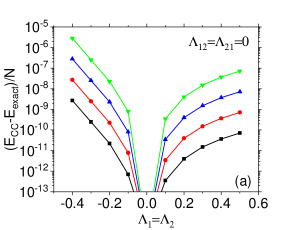
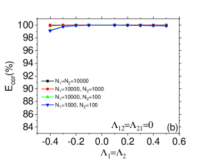
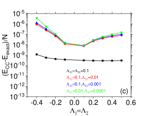
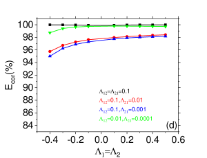
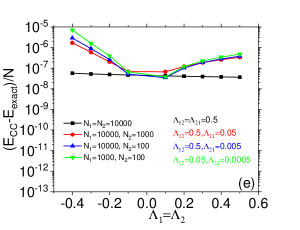
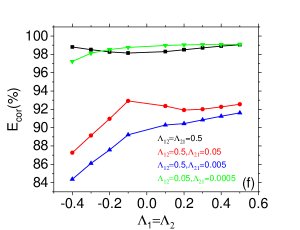
Figure 1: Variation of the difference between the coupled-cluster energy per particle and the corresponding analytical exact energy per particle, $\Delta_{\text{cc}}=\dfrac{E_{\text{cc}}-E_{\text{exact}}}{N}$, with respect to the intra-species interaction parameters $\Lambda_{1}=\Lambda_{2}$ is shown in panels (a), (c), and (e). Panels (b), (d), and (f) present $E_{\text{cor}}(\%)=\dfrac{E_{\text{MF}}-E_{\text{cc}}}{E_{\text{MF}}-E_{\text{exact}}}\times 100$ as a function of the intra-species interaction parameters. The coupled-cluster energy is calculated for the combinations of equal and unequal numbers of bosons of the two species: $N_{1}=N_{2}=10000$ (black squares), $N_{1}=10000$ and $N_{2}=1000$ (red circles), $N_{1}=10000$ and $N_{2}=100$ (blue triangles), and $N_{1}=1000$ and $N_{2}=100$ (green triangles). Captions are shown in panel (b) and (e). For panels in the first row, the two species are non-interacting to each other. Panels (a) and (b) serve for benchmarking the coupled-cluster theory for bosonic single species. In panels (c) to (f), $\Lambda_{12}$ and $\Lambda_{21}$ are demonstrated in the same color as their corresponding curves. Continuous curves are to guide the eye only. All the quantities are dimensionless.

In this work we concentrate on the energy and we examine two features, the variation of the difference between the CCSD-M energy per particle and the corresponding analytical exact energy per particle, $\Delta_{\text{cc}}=\dfrac{E_{\text{cc}}-E_{\text{exact}}}{N}$ (left column of Fig. 1) and the percentage of correlation energy, $E_{\text{cor}}(\%)=\dfrac{E_{\text{MF}}-E_{\text{cc}}}{E_{\text{MF}}-E_{\text{exact}}}\times 100$ (right column of Fig. 1) as a function of the intra-species interaction parameter. The figure presents the combinations of a balanced number of bosons of the two species $N_{1}=N_{2}=10000$, and imbalanced numbers of bosons, $N_{1}=10000$ and $N_{2}=1000$, $N_{1}=10000$ and $N_{2}=100$, and $N_{1}=1000$ and $N_{2}=100$. The inter-species interaction parameters, $\Lambda_{12}$ and $\Lambda_{21}$, are displayed in each panel. Note that the left and right columns correspond to each other with the same numbers of bosons and interaction parameters. Let us define the strength of the intra- and inter-species interactions. If $\lambda_{1}$, $\lambda_{2}$, and $\lambda_{12}$ are $<0.01$ the system is referred to as weakly interacting, in between $0.011$ and $0.05$ defines a medium strength interaction, and $>0.05$ is strong interaction. To remind the reader $\Lambda_{1}=\lambda_{1}(N_{1}-1)$, $\Lambda_{2}=\lambda_{2}(N_{2}-1)$, $\Lambda_{21}=\lambda_{12}N_{2}$, and $\Lambda_{12}=\lambda_{12}N_{1}$. Thus, the largest interaction parameter used in the examples below are: $\Lambda_{1}=10^{4}$, $\Lambda_{2}=10^{4}$, $\Lambda_{12}=50$, and $\Lambda_{21}=50$.

Before we are going to analyze the performance of the CCSD-M, let us take two species which are non-interacting to each other, $\Lambda_{12}=\Lambda_{21}=0$, and check the performance of the coupled cluster theory. For $\Lambda_{12}=\Lambda_{21}=0$, the coefficient $e_{22}=0$ and the performance of the coupled-cluster for mixtures boils down to the coupled-cluster for single species [47], see Eq. 54 for correlation energy. The benchmark presented here is very promising.

Fig. 1 (a) and (b) present $\Delta_{\text{cc}}$ and $E_{\text{cor}}(\%)$, respectively, for a basic situation when the two species are non-interacting to each other for several balanced and imbalanced combinations of boson numbers. It is found that the deviation $\Delta_{\text{cc}}$ is always less than $10^{-5}$ with, obviously, no deviation when $\Lambda_{1}=\Lambda_{2}=0$. Moreover, apart from $\Lambda_{1}=\Lambda_{2}=0$, for a fixed combination of bosons, balanced or imbalanced, the minimal $\Delta_{\text{cc}}$ occurs for the attractive inter-species interaction $\Lambda_{1}=\Lambda_{2}=+0.1$. Fig. 1 (b) shows that, for $\Lambda_{12}=\Lambda_{21}=0$, CCSD-M theory with two orbitals in each species can capture more than $99\%$ of the correlation energy, for the considered intra-species interaction parameters, which is very promising.

Now, when we switch on the inter-species interaction parameters, see Figs. 1 (c) and (d), $\Delta_{\text{cc}}$ varies approximately from $10^{-5}$ to $10^{-9}$, and the corresponding $E_{\text{cor}}(\%)$ deviates between $0.01\%$ to $5\%$ from the exact correlation energy. As we further increase of $\Lambda_{12}$ and $\Lambda_{21}$ five times for each cases, $\Delta_{\text{cc}}$ is around $10^{-5}-10^{-7}$, see Fig. 1 (e). Moreover, the coupled-cluster theory with $M_{1}=M_{2}=2$ can capture more than $84\%$ of correlation energy. Naturally, for strong inter-species interaction, one requires more orbitals to incorporate the accurate correlation energy. All in all, Fig. 1 exhibits that we require either an additional number of orbitals, or a higher order of excitations, or the combination of both to get the full correlation energy in the particle imbalanced cases with repulsive intra-species interaction parameter.

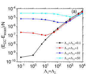
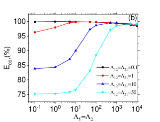
Figure 2: Variation of (a) the difference between the coupled-cluster energy per particle and the corresponding analytical exact energy per particle, $\Delta_{\text{cc}}=\dfrac{E_{\text{cc}}-E_{\text{exact}}}{N}$, and (b) $E_{\text{cor}}(\%)=\dfrac{E_{\text{MF}}-E_{\text{cc}}}{E_{\text{MF}}-E_{\text{exact}}}\times 100$ as a function of intra-species interaction parameters $\Lambda_{1}=\Lambda_{2}$. The coupled-cluster energy is calculated for the numbers of bosons $N_{1}=N_{2}=10000$. Results are presented for the inter-species interaction parameters, $\Lambda_{12}$ and $\Lambda_{21}$, 0.1, 1, 10, and 50. It is found that if we increase both intra- and inter-species interaction parameters, CCSD-M can capture higher fractions of the correlation energy. All the quantities are dimensionless.

Till now, the CCSD-M approach shows excellent success for weakly interacting bosonic mixtures. Here, we check the applicability of the CCSD-M theory for a strongly interacting system with a large number of bosons in the two species. Fig. 2 exhibits (a) $\Delta_{\text{cc}}=\dfrac{E_{\text{cc}}-E_{\text{exact}}}{N}$ and (b) $E_{\text{cor}}(\%)$ for $N_{1}=N_{2}=10000$ with various inter-species interaction parameters ranging from weak to medium, namely, 0.1, 1, 10, and 50, while the intra-species interaction parameters vary from weak $10^{-2}$ to strong $10^{4}$. For weak $\Lambda_{12}=\Lambda_{21}=0.1$, $\Delta_{\text{cc}}$ increases with the values of $\Lambda_{1}$ and $\Lambda_{2}$. Interestingly, for comparatively stronger values $\Lambda_{12}=\Lambda_{21}=1$, $10$, and $50$, we observe that $\Delta_{\text{cc}}$ decreases at the beginning and then increases with the intra-species interaction parameter. This change in nature and the crossing of $\Delta_{\text{cc}}$ curves correlates with the $E_{\text{cc}}-E_{\text{MF}}$. On the whole, we observe that $\Delta_{\text{cc}}<10^{-4}$ even for strong intra- and inter-species interaction strengths with a large number of bosons in each species which proves the remarkable success of CCSD-M theory.

Now we discuss how much of the correlation energy is captured by the CCSD-M with the number of orbitals $M_{1}=M_{2}=2$, see Fig. 2 (b). When the inter-species interaction is weak, $\Lambda_{12}=\Lambda_{21}=0.1$, the coupled-cluster theory can determine more than $98\%$ of the correlation energy for the weak to strong intra-species interaction parameters. The correlation energy deviates from the exact results as one increases the inter-species interaction. For inter-species interaction satisfying $\Lambda_{12}=\Lambda_{21}\geq 1$, it is interesting to see that, when the inter- and intra-species interactions are of the same order, the CCSD-M theory with $M_{1}=M_{2}=2$ orbitals captures more than about $85\%$ of correlation energy. Moreover, we observe that for strong values of the intra-species interactions $\Lambda_{1}=\Lambda_{2}$, two orbitals for each species can produce more than $97.5\%$ of the correlation energy, which exhibits the potential of coupled-cluster theory for mixtures.

VI Conclusions

In this work, we present the theoretical development and implementation details of the coupled-cluster theory for the bosonic mixture of binary species, with the numbers of bosons $N_{1}$ and $N_{2}$ for species-1 and species-2, respectively, in external trap potentials. In the coupled-cluster theory for mixtures, the ansatz of the many-body wavefunction is obtained when the three exponential cluster operators $e^{T^{(1)}}$, $e^{T^{(2)}}$, and $e^{T^{(12)}}$, are applied onto the ground configuration. Since $T^{(1)}$, $T^{(2)}$, and $T^{(12)}$ commute with each other, their exponents can be separated. Here, $T^{(12)}=0$ implies that there is no inter-species interaction between the two bosonic species and the theory derived here boils down to a single-species coupled-cluster ansatz for each of the species. $T^{(1)}$ and $T^{(2)}$ incorporate the single, double, triple, … excitations in each species, while $T^{(12)}$ starts from the double excitations, one for each species. As per the bosons statistics, there is no restriction in occupying a particular orbital for bosons. Our starting point for building up correlations is the standard mean-field for which $N_{1}$ bosons occupy one orbital of species-1 and $N_{2}$ bosons are sitting in another orbital of species-2. These orbitals are obtained by the solution of the coupled Gross-Pitaeveskii equations of the mixtures.

Next, we have derived the involved working equations for the unknown coefficients in the coupled-cluster theory for bosonic mixtures using an arbitrary sets of orthonormal orbitals. Also, the comparatively simplified version of the working equations are derived for the coefficients using Fock-like operators. The working equations with Fock-like operators as well as those for an arbitrary sets of orthonormal orbitals consist of $M_{1}-1$ and $M_{2}-1$ equations for single excitations in species-1 and species-2, respectively, $M_{1}(M_{1}-1)/2$ and $M_{2}(M_{2}-1)/2$ equations for double excitations in species-1 and species-2, respectively, and $(M_{1}-1)(M_{2}-1)$ equations for simultaneous excitations in the two species, and so on. Utilizing orthonormal orbitals, we find that the correlation energy for the mixture depends on the different coefficients, namely, $\{c_{s}\}$, $\{d_{l}\}$, $\{c_{rs}\}$, $\{d_{kl}\}$, and $\{e_{ls}\}$, which originate for the single and double excitations only.

Furthermore, we have implemented our developed coupled-cluster theory on the harmonic interaction model for mixtures and compared the results with this exactly solvable many-body model for the different strengths of the inter-species and intra-species interactions. The investigation serves to check the theory, implementation, and the usage of the theory, that is the truncation to CCSD-M and the inclusion of $M_{1}=M_{2}=2$, for the studied examples. We have calculated the energy for the mixture with $N_{1}$ and $N_{2}$ ranging from 100 to 10000 bosons, and in various scenarios for balanced and imbalanced numbers of bosons between the two species. To check the performance of our theory, we calculated the difference between the coupled-cluster energy per particle and the corresponding analytical exact energy per particle, $\Delta_{\text{cc}}=\dfrac{E_{\text{cc}}-E_{\text{exact}}}{N}$. We have shown how much of the exact correlation energy can be captured by the coupled-cluster theory by calculating $E_{\text{cor}}(\%)=\dfrac{E_{\text{MF}}-E_{\text{cc}}}{E_{\text{MF}}-E_{\text{exact}}}\times 100$. We found that even for rather strong intra- and inter-species interactions and relatively large numbers of bosons for each species $N_{1}=N_{2}=10^{4}$, the CCSD-M provides remarkable success.

Before ending this section, it is worthwhile to mention the computational scaling of the CCSD-M approach in comparison to the configuration interaction which employs a basis set expansion [60]. For example, the largest system we have in our work is 10000 bosons in each species which produces $10001^{2}\approx 10^{8}$ coefficients for configuration interaction with two orbitals per species. While, there are only three coefficients for CCSD-M. For more number of bosons, the number of coefficients increases for configuration interaction accordingly. This analysis is impressive in terms of saving computational resources with respect to configuration interaction and it shows the excellent applicability of CCSD-M approach. The quality of coupled-cluster theory opens the way to investigate few- to many-boson binary mixture up to fairly strong interaction strengths where several orbitals, or higher order excitations, or both of them are required to describe the physics accurately.

All in all, it is found that the coupled-cluster theory for bosonic mixtures is a promising many-body approach. As an outlook, one could be interested to investigate various properties of bosonic mixtures for other external potentials and inter-bosons interactions [28]. For instance, one can compute the reduced one-particle density matrix of each species from the CC-M wavefunction, and from them the respective eigenvalues. This will tell one how the condensate fraction of each species is modified by the inter-species and intra-species interactions. Also, it would be interesting to extract from the CC-M wavefunction the entanglement between species-1 and species-2. Examining the CC-M ansatz Eqs. 5 and 6, it is clear that the cluster operator $T^{(12)}$ alone governs the entanglement between the two species. Moreover, one can determine the expectation value of an operator, $\Omega$, using the so-called $\Lambda$-equation, $\langle\Omega\rangle=\langle\phi_{0}|(1+\Lambda)e^{-T}\Omega e^{T}|\phi_{0}\rangle$, where $\Lambda$ is the Lagrange multiplier [61]. For that, the equation of motion for $\Lambda$ would have to be derived. Based on our CCSD-M, one can anticipate the development of a time-dependent coupled-cluster theory for bosons first, and then one could expect to expand and explore the dynamics of bosonic mixtures using time-dependent coupled-cluster. This is a challenge to be undertaken in future research. We believe that fermionic time-dependent coupled-cluster theory will be helpful in this direction [62, 63].

Data Availability

The data that support the findings of this work are available from the corresponding author upon reasonable request.

Appendix

A. Relations between one-body and two-body terms

Using the eigenvalue-equations of the Fock-like operators, ${F}_{1}\varphi_{i}=\mu_{i}^{(1)}\varphi_{i}$ and ${F}_{2}\psi_{i}=\mu_{i}^{(2)}\psi_{i}$, described in the main text [Eqs. III and  III ], one can find a few relations between one-body and two-body terms which can assist in simplifying the working equations of the coupled-cluster theory for bosonic mixtures. The relations are as follows

$$h_{\bar{1}\bar{1}}^{(1)}+(N_{1}-1)V_{\bar{1}\bar{1}\bar{1}\bar{1}}^{(1)}+N_{2}V_{\bar{1}1\bar{1}1}^{(12)}=\mu_{1}^{(1)},$$

$$h_{11}^{(2)}+(N_{2}-1)V_{1111}^{(2)}+N_{1}V_{\bar{1}1\bar{1}1}^{(12)}=\mu_{1}^{(2)},$$

$$\sum_{s=2}^{M_{1}}\Big{[}h_{\bar{s}\bar{s}}^{(1)}+(N_{1}-1)V_{\bar{s}\bar{1}\bar{s}\bar{1}}^{(1)}+N_{2}V_{\bar{s}1\bar{s}1}^{(12)}\Big{]}=\mu_{s}^{(1)},$$

$$\sum_{l=2}^{M_{2}}\Big{[}h_{ll}^{(2)}+(N_{2}-1)V_{l1l1}^{(2)}+N_{1}V_{\bar{1}l\bar{1}l}^{(12)}\Big{]}=\mu_{l}^{(2)},$$

$$\sum_{s=2}^{M_{1}}\Big{[}h_{\bar{1}\bar{s}}^{(1)}+(N_{1}-1)V_{\bar{1}\bar{1}\bar{s}\bar{1}}^{(1)}+N_{2}V_{\bar{1}1\bar{s}1}^{(12)}\Big{]}=0,$$

$$\sum_{l=2}^{M_{2}}\Big{[}h_{1l}^{(2)}+(N_{2}-1)V_{11l1}^{(2)}+N_{1}V_{\bar{1}1\bar{1}l}^{(12)}\Big{]}=0,$$

$$\sum_{s=2}^{M_{1}}\Big{[}h_{\bar{s}\bar{1}}^{(1)}+(N_{1}-1)V_{\bar{s}\bar{1}\bar{1}\bar{1}}^{(1)}+N_{2}V_{\bar{s}1\bar{1}1}^{(12)}\Big{]}=0,$$

$$\sum_{l=2}^{M_{2}}\Big{[}h_{l1}^{(2)}+(N_{2}-1)V_{l111}^{(2)}+N_{1}V_{\bar{1}l\bar{1}1}^{(12)}\Big{]}=0.$$ (A.1)

The first two relations are obtained when the ground orbital is sandwiching in Eq. III the Fock operator. Similarly, the third and fourth relations are found when the same excited orbitals act on the Fock operator from the left and right sides. We get the other relations when ground and excited orbitals are sandwiching the Fock operator in Eq. III. The first four relations involve chemical potentials for the ground and virtual orbitals as the Hamiltonian is sandwiched between the same two orbitals.

B. Transformed creation and destruction operators

The derivation of the working equations of the coupled-cluster theory for bosonic mixtures demands the transformation of the creation operators of the ground orbitals, $\dot{a}_{{1}}^{\dagger}=a_{{1}}^{\dagger}-\mathcal{K}_{{1}}$ and $\dot{b}_{1}^{\dagger}=b_{1}^{\dagger}-\mathcal{L}_{1}$, and of the destruction operators of the virtual orbitals, $\dot{a}_{p}=a_{p}-\mathcal{K}_{p}$ and $\dot{b}_{i}=b_{i}-\mathcal{L}_{i}$, for both species. The explicit expansions of the first few terms of $\mathcal{K}_{{1}}$, $\mathcal{K}_{{p}}$, $\mathcal{L}_{1}$, and $\mathcal{L}_{i}$ read

$$\mathcal{K}_{{1}} = \sum_{p=2}^{M_{1}}c_{p}a_{p}^{\dagger}+2\sum_{p,q=2}^{M_{1}}c_{pq}a_{p}^{\dagger}a_{q}^{\dagger}a_{1}+3\sum_{p,q,r=2}^{M_{1}}c_{pqr}a_{p}^{\dagger}a_{q}^{\dagger}a_{r}^{\dagger}a_{1}^{2}+...$$ (B.1)

$$+ \sum_{p=2}^{M_{1}}\sum_{i=2}^{M_{2}}e_{pi}a_{p}^{\dagger}b_{i}^{\dagger}b_{1}+2\sum_{p,q=2}^{M_{1}}\sum_{i=2}^{M_{2}}e_{pqi}a_{p}^{\dagger}a_{q}^{\dagger}b_{i}^{\dagger}a_{1}b_{1}+\sum_{p=2}^{M_{1}}\sum_{i,j=2}^{M_{2}}e_{pij}a_{p}^{\dagger}b_{i}^{\dagger}b_{j}^{\dagger}b_{1}^{2}+...,$$

$$\mathcal{K}_{p} = c_{p}a_{1}+2\sum_{q=2}^{M_{1}}c_{pq}a_{q}^{\dagger}a_{1}^{2}+3\sum_{q,r=2}^{M_{1}}c_{pqr}a_{q}^{\dagger}a_{r}^{\dagger}a_{1}^{3}+...$$ (B.2)

$$+ \sum_{i=2}^{M_{2}}e_{pi}b_{i}^{\dagger}a_{1}b_{1}+2\sum_{q=2}^{M_{1}}\sum_{i=2}^{M_{2}}e_{pqi}a_{q}^{\dagger}b_{i}^{\dagger}a_{1}^{2}b_{1}+\sum_{i,j=2}^{M_{2}}e_{pij}b_{i}^{\dagger}b_{j}^{\dagger}a_{1}b_{1}^{2}+...,$$

$$\mathcal{L}_{1} = \sum_{i=2}^{M_{2}}d_{i}b_{i}^{\dagger}+2\sum_{i,j=2}^{M_{2}}d_{ij}b_{i}^{\dagger}b_{j}^{\dagger}b_{1}+3\sum_{i,j,k=2}^{M_{2}}d_{ijk}b_{i}^{\dagger}b_{j}^{\dagger}b_{k}^{\dagger}b_{1}^{2}+...$$ (B.3)

$$+ \sum_{p=2}^{M_{1}}\sum_{i=2}^{M_{2}}e_{pi}a_{p}^{\dagger}b_{i}^{\dagger}a_{1}+2\sum_{p=2}^{M_{1}}\sum_{i,j=2}^{M_{2}}e_{pij}a_{p}^{\dagger}b_{i}^{\dagger}b_{j}^{\dagger}a_{1}b_{1}+\sum_{p,q=2}^{M_{1}}\sum_{i=2}^{M_{2}}e_{pqi}a_{p}^{\dagger}a_{q}^{\dagger}b_{i}^{\dagger}a_{1}^{2}+...,$$

$$\mathcal{L}_{i} = d_{i}b_{1}+2\sum_{j=2}^{M_{2}}d_{ij}b_{j}^{\dagger}b_{1}^{2}+3\sum_{j,k=2}^{M_{2}}d_{ijk}b_{j}^{\dagger}b_{k}^{\dagger}b_{1}^{3}+...$$ (B.4)

$$+ \sum_{p=2}^{M_{1}}e_{pi}a_{p}^{\dagger}a_{1}b_{1}+2\sum_{p=2}^{M_{1}}\sum_{j=2}^{M_{2}}e_{pij}a_{p}^{\dagger}b_{j}^{\dagger}a_{1}b_{1}^{2}+\sum_{p,q=2}^{M_{1}}e_{pqi}a_{p}^{\dagger}a_{q}^{\dagger}a_{1}^{2}b_{1}+....$$

The above mentioned expansions are used to find out the unknown coefficients, $c_{p_{1}p_{2}...p_{n}}$, $d_{i_{1}i_{2}...i_{m}}$, and $e_{p_{1}...p_{n^{\prime}}i_{1}...i_{m^{\prime}}}$.

C. Transformed two-body operators

The transformed intra-species and inter-species two-body operators $\dot{V}^{(1)}$, $\dot{V}^{(2)}$, and $\dot{V}^{(12)}$ are required to solve the coupled-cluster energy, see Sec. IVB, by finding out the unknown coefficients. $\dot{V}^{(1)}$ consists of nine terms listed below when each term is a combination of the creation and destruction operators of species-1. The nine terms are as follows

$$\dot{V}^{(1)}=\sum_{w=1}^{9}\dot{V}^{(1)}(w),$$

$$\dot{V}^{(1)}(1)=\dfrac{1}{2}V_{\bar{1}\bar{1}\bar{1}\bar{1}}^{(1)}\dot{a}_{1}^{\dagger}\dot{a}_{1}^{\dagger}a_{1}a_{1},\hskip 48.36958pt\dot{V}^{(1)}(2)=\sum_{s=2}^{M_{1}}V_{\bar{1}\bar{1}\bar{1}\bar{s}}^{(1)}\dot{a}_{1}^{\dagger}\dot{a}_{1}^{\dagger}a_{1}\dot{a}_{s},$$

$$\dot{V}^{(1)}(3)=\sum_{s=2}^{M_{1}}V_{\bar{s}\bar{1}\bar{1}\bar{1}}^{(1)}a_{s}^{\dagger}\dot{a}_{1}^{\dagger}a_{1}a_{1},\hskip 41.25641pt\dot{V}^{(1)}(4)=\dfrac{1}{2}\sum_{r,s=2}^{M_{1}}V_{\bar{1}\bar{1}\bar{r}\bar{s}}^{(1)}\dot{a}_{1}^{\dagger}\dot{a}_{1}^{\dagger}\dot{a}_{r}\dot{a}_{s},$$

$$\dot{V}^{(1)}(5)=\dfrac{1}{2}\sum_{r,s=2}^{M_{1}}V_{\bar{r}\bar{s}\bar{1}\bar{1}}^{(1)}a_{r}^{\dagger}a_{s}^{\dagger}a_{1}a_{1},\hskip 28.45274pt\dot{V}^{(1)}(6)=\sum_{r,s=2}^{M_{1}}(V_{\bar{1}\bar{r}\bar{1}\bar{s}}^{(1)}+V_{\bar{1}\bar{r}\bar{s}\bar{1}}^{(1)})\dot{a}_{1}^{\dagger}a_{r}^{\dagger}a_{1}\dot{a}_{s},$$

$$\dot{V}^{(1)}(7)=\sum_{q,r,s=2}^{M_{1}}V_{\bar{1}\bar{q}\bar{r}\bar{s}}^{(1)}\dot{a}_{1}^{\dagger}a_{q}^{\dagger}\dot{a}_{r}\dot{a}_{s},\hskip 35.56593pt\dot{V}^{(1)}(8)=\sum_{q,r,s=2}^{M_{1}}V_{\bar{q}\bar{r}\bar{s}\bar{1}}^{(1)}a_{q}^{\dagger}a_{r}^{\dagger}\dot{a}_{s}a_{{1}},$$

$$\dot{V}^{(1)}(9)=\dfrac{1}{2}\sum_{p,q,r,s=2}^{M_{1}}V_{\bar{p}\bar{q}\bar{r}\bar{s}}^{(1)}a_{p}^{\dagger}a_{q}^{\dagger}\dot{a}_{r}\dot{a}_{s}.$$ (C.1)

Similarly, $\dot{V}^{(2)}$ has nine terms and each term carries the creation and destruction operators of species-2. The nine terms read

$$\dot{V}^{(2)}=\sum_{w=1}^{9}\dot{V}^{(2)}(w),$$

$$\dot{V}^{(2)}(1)=\dfrac{1}{2}V_{1111}^{(2)}\dot{b}_{1}^{\dagger}\dot{b}_{1}^{\dagger}b_{1}b_{1},\hskip 46.94687pt\dot{V}^{(2)}(2)=\sum_{l=2}^{M_{2}}V_{111l}^{(2)}\dot{b}_{1}^{\dagger}\dot{b}_{1}^{\dagger}b_{1}\dot{b}_{l},$$

$$\dot{V}^{(2)}(3)=\sum_{l=2}^{M_{2}}V_{l111}^{(2)}b_{l}^{\dagger}\dot{b}_{1}^{\dagger}b_{1}b_{1},\hskip 42.67912pt\dot{V}^{(2)}(4)=\dfrac{1}{2}\sum_{k,l=2}^{M_{2}}V_{11kl}^{(2)}\dot{b}_{1}^{\dagger}\dot{b}_{1}^{\dagger}\dot{b}_{k}\dot{b}_{l},$$

$$\dot{V}^{(2)}(5)=\dfrac{1}{2}\sum_{k,l=2}^{M_{2}}V_{kl11}^{(2)}b_{k}^{\dagger}b_{l}^{\dagger}b_{1}b_{1},\hskip 28.45274pt\dot{V}^{(2)}(6)=\sum_{k,l=2}^{M_{2}}(V_{1k1l}^{(2)}+V_{1kl1}^{(2)})\dot{b}_{1}^{\dagger}b_{k}^{\dagger}b_{1}\dot{b}_{l},$$

$$\dot{V}^{(2)}(7)=\sum_{j,k,l=2}^{M_{2}}V_{1jkl}^{(2)}\dot{b}_{1}^{\dagger}b_{j}^{\dagger}\dot{b}_{k}\dot{b}_{l},\hskip 36.98866pt\dot{V}^{(2)}(8)=\sum_{j,k,l=2}^{M_{2}}V_{jkl1}^{(2)}b_{j}^{\dagger}b_{k}^{\dagger}\dot{b}_{l}b_{1},$$

$$\dot{V}^{(2)}(9)=\dfrac{1}{2}\sum_{i,j,k,l=2}^{M_{2}}V_{ijkl}^{(2)}b_{i}^{\dagger}b_{j}^{\dagger}\dot{b}_{k}\dot{b}_{l}.$$ (C.2)

$\dot{V}^{(12)}$ is made of sixteen terms and each of the terms is a mixture of the creation and destruction operators of species-1 and species-2. All sixteen terms can be readily found as

$$\dot{V}^{(12)}=\sum_{w=1}^{16}\dot{V}^{(12)}(w),$$

$$\dot{V}^{(12)}(1)=V_{\bar{1}1\bar{1}1}^{(12)}\dot{a}_{1}^{\dagger}\dot{b}_{1}^{\dagger}a_{1}b_{1},\hskip 62.59596pt\dot{V}^{(12)}(2)=\sum_{l=2}^{M_{2}}V_{\bar{1}1\bar{1}l}^{(12)}\dot{a}_{1}^{\dagger}\dot{b}_{1}^{\dagger}a_{1}\dot{b}_{l},$$

$$\dot{V}^{(12)}(3)=\sum_{s=2}^{M_{1}}V_{\bar{1}1\bar{s}1}^{(12)}\dot{a}_{1}^{\dagger}\dot{b}_{1}^{\dagger}\dot{a}_{s}b_{1},\hskip 46.94687pt\dot{V}^{(12)}(4)=\sum_{l=2}^{M_{2}}V_{\bar{1}l\bar{1}1}^{(12)}\dot{a}_{1}^{\dagger}b_{l}^{\dagger}a_{1}b_{1},$$

$$\dot{V}^{(12)}(5)=\sum_{s=2}^{M_{1}}V_{\bar{s}1\bar{1}1}^{(12)}a_{s}^{\dagger}\dot{b}_{1}^{\dagger}a_{1}b_{1},\hskip 46.94687pt\dot{V}^{(12)}(6)=\sum_{s=2}^{M_{1}}\sum_{l=2}^{M_{2}}V_{\bar{1}1\bar{s}l}^{(12)}\dot{a}_{1}^{\dagger}\dot{b}_{1}^{\dagger}\dot{a}_{s}\dot{b}_{l},$$

$$\dot{V}^{(12)}(7)=\sum_{s=2}^{M_{1}}\sum_{l=2}^{M_{2}}V_{\bar{s}l\bar{1}1}^{(12)}a_{s}^{\dagger}b_{l}^{\dagger}a_{1}b_{1},\hskip 31.2982pt\dot{V}^{(12)}(8)=\sum_{r,s=2}^{M_{1}}V_{\bar{r}1\bar{s}1}^{(12)}a_{r}^{\dagger}\dot{b}_{1}^{\dagger}\dot{a}_{s}b_{1},$$

$$\dot{V}^{(12)}(9)=\sum_{k,l=2}^{M_{2}}V_{\bar{1}k\bar{1}l}^{(12)}\dot{a}_{1}^{\dagger}b_{k}^{\dagger}a_{1}\dot{b}_{l},\hskip 46.94687pt\dot{V}^{(12)}(10)=\sum_{s=2}^{M_{1}}\sum_{l=2}^{M_{2}}V_{\bar{s}1\bar{1}l}^{(12)}a_{s}^{\dagger}\dot{b}_{1}^{\dagger}a_{1}\dot{b}_{l},$$

$$\dot{V}^{(12)}(11)=\sum_{s=2}^{M_{1}}\sum_{l=2}^{M_{2}}V_{\bar{1}l\bar{s}1}^{(12)}\dot{a}_{1}^{\dagger}b_{l}^{\dagger}\dot{a}_{s}b_{1},\hskip 28.45274pt\dot{V}^{(12)}(12)=\sum_{s=2}^{M_{1}}\sum_{k,l=2}^{M_{2}}V_{\bar{1}k\bar{s}l}^{(12)}\dot{a}_{1}^{\dagger}b_{k}^{\dagger}\dot{a}_{s}\dot{b}_{l},$$

$$\dot{V}^{(12)}(13)=\sum_{r,s=2}^{M_{1}}\sum_{l=2}^{M_{2}}V_{\bar{r}1\bar{s}l}^{(12)}a_{r}^{\dagger}\dot{b}_{1}^{\dagger}\dot{a}_{s}\dot{b}_{l},\hskip 28.45274pt\dot{V}^{(12)}(14)=\sum_{s=2}^{M_{1}}\sum_{k,l=2}^{M_{2}}V_{\bar{s}k\bar{1}l}^{(12)}a_{s}^{\dagger}b_{k}^{\dagger}a_{1}\dot{b}_{l},$$

$$\dot{V}^{(12)}(15)=\sum_{r,s=2}^{M_{1}}\sum_{l=2}^{M_{2}}V_{\bar{r}l\bar{s}1}^{(12)}a_{r}^{\dagger}b_{l}^{\dagger}\dot{a}_{s}b_{1},\hskip 28.45274pt\dot{V}^{(12)}(16)=\sum_{r,s=2}^{M_{1}}\sum_{k,l=2}^{M_{2}}V_{\bar{r}k\bar{s}l}^{(12)}a_{r}^{\dagger}b_{k}^{\dagger}\dot{a}_{s}\dot{b}_{l}.$$ (C.3)

The working equations of the coupled-cluster theory for bosonic mixtures are developed using the transformed two-body operators along with $\dot{H}_{0}$, see Eq. 16.

D. The general working equations

Here we present the general forms of the working equations of the coupled-cluster theory for bosonic mixtures. The derivation of the coupled working equations is very lengthy and involved. We start with the single excitation in both species by solving the equations $\langle\phi_{0}|a_{1}^{\dagger}a_{\bar{i}}\dot{H}|\phi_{0}\rangle=0$ and $\langle\phi_{0}|b_{1}^{\dagger}b_{i}\dot{H}|\phi_{0}\rangle=0$ where $\bar{i}=2,3,...,M_{1}$ and $i=2,3,...,M_{2}$. The general form of the single excitation in species-1 can be readily obtained as

$$0 = -h_{\bar{1}\bar{1}}^{(1)}c_{\bar{i}}+(N_{1}-1)\sum_{s=2}^{M_{1}}h_{\bar{1}\bar{s}}^{(1)}(2c_{s\bar{i}})-\sum_{s=2}^{M_{1}}h_{\bar{1}\bar{s}}^{(1)}(c_{\bar{i}}c_{s})+h_{\bar{i}\bar{1}}^{(1)}+\sum_{s=2}^{M_{1}}h_{\bar{i}\bar{s}}^{(1)}c_{s}+N_{2}\sum_{l=2}^{M_{2}}h_{1l}^{(2)}e_{\bar{i}l}$$ (D.1)

$$-(N_{1}-1)V_{\bar{1}\bar{1}\bar{1}\bar{1}}^{(1)}c_{\bar{i}}+(N_{1}-1)(N_{1}-2)\sum_{s=2}^{M_{1}}V_{\bar{1}\bar{1}\bar{1}\bar{s}}^{(1)}(2c_{s\bar{i}})-2(N_{1}-1)\sum_{s=2}^{M_{1}}V_{\bar{1}\bar{1}\bar{1}\bar{s}}^{(1)}(c_{\bar{i}}c_{s})+(N_{1}-1)V_{\bar{i}\bar{1}\bar{1}\bar{1}}^{(1)}$$

$$+\sum_{r,s=2}^{M_{1}}V_{\bar{1}\bar{1}\bar{r}\bar{s}}^{(1)}\bar{\alpha}_{rs\bar{i}}+(N_{1}-1)\Bigg{[}\sum_{s=2}^{M_{1}}(V_{\bar{1}\bar{i}\bar{1}\bar{s}}^{(1)}+V_{\bar{1}\bar{i}\bar{s}\bar{1}}^{(1)})c_{s}\Bigg{]}+(N_{1}-1)\Bigg{[}\sum_{r,s=2}^{M_{1}}V_{\bar{1}\bar{i}\bar{r}\bar{s}}^{(1)}(2c_{rs}+c_{r}c_{s})\Bigg{]}$$

$$+N_{2}(N_{2}-1)\sum_{l=2}^{M_{2}}V_{111l}^{(2)}e_{\bar{i}l}+\dfrac{1}{2}N_{2}(N_{2}-1)\sum_{k,l=2}^{M_{2}}V_{11kl}^{(2)}(2e_{\bar{i}lk}+e_{\bar{i}k}d_{l}+e_{\bar{i}l}d_{k})$$

$$-N_{2}V_{\bar{1}1\bar{1}1}^{(12)}c_{\bar{i}}+(N_{1}-1)N_{2}\sum_{l=2}^{M_{2}}V_{\bar{1}1\bar{1}l}^{(12)}e_{\bar{i}l}-N_{2}\sum_{l=2}^{M_{2}}V_{\bar{1}1\bar{1}l}^{(12)}c_{\bar{i}}d_{l}$$

$$+N_{2}\Bigg{[}(N_{1}-1)\sum_{s=2}^{M_{1}}V_{\bar{1}1\bar{s}1}^{(12)}(2c_{s\bar{i}})-\sum_{s=2}^{M_{1}}V_{\bar{1}1\bar{s}1}^{(12)}(c_{\bar{i}}c_{s})+V_{\bar{i}1\bar{1}1}^{(12)}\Bigg{]}$$

$$+(N_{1}-1)N_{2}\sum_{s=2}^{M_{1}}\sum_{l=2}^{M_{2}}V_{\bar{1}1\bar{s}l}^{(12)}(2e_{\bar{i}sl}+c_{s}e_{\bar{i}l}+2c_{s\bar{i}}d_{l})-N_{2}\sum_{s=2}^{M_{1}}\sum_{l=2}^{M_{2}}V_{\bar{1}1\bar{s}l}^{(12)}(c_{\bar{i}}e_{sl}+c_{\bar{i}}c_{s}d_{l})$$

$$+N_{2}\Bigg{[}\sum_{s=2}^{M_{1}}V_{\bar{i}1\bar{s}1}^{(12)}c_{s}+\sum_{l=2}^{M_{2}}V_{\bar{i}1\bar{1}l}^{(12)}d_{l}+\sum_{s=2}^{M_{1}}\sum_{l=2}^{M_{2}}V_{\bar{i}1\bar{s}l}^{(12)}(e_{sl}+c_{s}d_{l})\Bigg{]}.$$

To calculate Eq. D.1, contributions from the fifth, seventh, and eighth terms of $\dot{H}_{0}$ in Eq. 16, the second, third, fifth, sixth, seventh, eighth, and ninth terms of $\dot{V}^{(2)}$ in Eq. C. Transformed two-body operators, and from the fourth, seventh, ninth, eleventh, twelfth, fourteenth, fifteenth, and sixteenth terms of $\dot{V}^{(12)}$ in Eq. C. Transformed two-body operators are zero due to the creation operators for virtual orbitals in the species-2. Also the fifth, eighth, and ninth terms of $\dot{V}^{(1)}$ in Eq. C. Transformed two-body operators do not have any contribution as they all exhibit two creation operators for virtual orbitals of species-1.

The general form of the single excitation in species-2 reads

$$0 = -h_{11}^{(2)}d_{i}+(N_{2}-1)\sum_{l=2}^{M_{2}}h_{1l}^{(2)}(2d_{li})-\sum_{l=2}^{M_{2}}h_{1l}^{(2)}(d_{i}d_{l})+h_{i1}^{(2)}+\sum_{l=2}^{M_{2}}h_{il}^{(2)}d_{l}+N_{1}\sum_{s=2}^{M_{1}}h_{\bar{1}\bar{s}}^{(1)}e_{si}$$ (D.2)

$$-(N_{2}-1)V_{1111}^{(2)}d_{i}+(N_{2}-1)(N_{2}-2)\sum_{l=2}^{M_{2}}V_{111l}^{(2)}(2d_{li})-2(N_{2}-1)\sum_{l=2}^{M_{2}}V_{111l}^{(2)}(d_{i}d_{l})+(N_{2}-1)V_{i111}^{(2)}$$

$$+\sum_{k,l=2}^{M_{2}}V_{11kl}^{(2)}\alpha_{kli}+(N_{2}-1)\Bigg{[}\sum_{l=2}^{M_{2}}(V_{1i1l}^{(2)}+V_{1il1}^{(2)})d_{l}\Bigg{]}+(N_{2}-1)\Bigg{[}\sum_{k,l=2}^{M_{2}}V_{1ikl}^{(2)}(2d_{lk}+d_{k}d_{l})\Bigg{]}$$

$$+N_{1}(N_{1}-1)\sum_{s=2}^{M_{1}}V_{\bar{1}\bar{1}\bar{1}\bar{s}}^{(1)}e_{si}+\dfrac{1}{2}N_{1}(N_{1}-1)\sum_{r,s=2}^{M_{1}}V_{\bar{1}\bar{1}\bar{r}\bar{s}}^{(1)}(2e_{sri}+e_{ri}c_{s}+e_{si}c_{r})$$

$$-N_{1}V_{\bar{1}1\bar{1}1}^{(12)}d_{i}+N_{1}(N_{2}-1)\sum_{s=2}^{M_{1}}V_{\bar{1}1\bar{s}1}^{(12)}e_{si}-N_{1}\sum_{s=2}^{M_{1}}V_{\bar{1}1\bar{s}1}^{(12)}d_{i}c_{s}$$

$$+N_{1}\Bigg{[}(N_{2}-1)\sum_{l=2}^{M_{2}}V_{\bar{1}1\bar{1}l}^{(12)}(2d_{li})-\sum_{l=2}^{M_{2}}V_{\bar{1}1\bar{1}l}^{(12)}(d_{i}d_{l})+V_{\bar{1}i\bar{1}1}^{(12)}\Bigg{]}$$

$$+N_{1}(N_{2}-1)\sum_{s=2}^{M_{1}}\sum_{l=2}^{M_{2}}V_{\bar{1}1\bar{s}l}^{(12)}(2e_{sli}+2c_{s}d_{li}+d_{l}e_{si})-N_{1}\sum_{s=2}^{M_{1}}\sum_{l=2}^{M_{2}}V_{\bar{1}1\bar{s}l}^{(12)}(d_{i}e_{sl}+d_{i}c_{s}+d_{l})$$

$$+N_{1}\Bigg{[}\sum_{s=2}^{M_{1}}V_{\bar{1}i\bar{s}1}^{(12)}c_{s}+\sum_{l=2}^{M_{2}}V_{\bar{1}i\bar{1}l}^{(12)}d_{l}+\sum_{s=2}^{M_{1}}\sum_{l=2}^{M_{2}}V_{\bar{1}i\bar{s}l}^{(12)}(e_{sl}+c_{s}d_{l})\Bigg{]}.$$

In order to determine Eq. D.2, the first, third, and fourth terms of $\dot{H}_{0}$ in Eq. 16, the second, third, fifth, sixth, seventh, eighth, and ninth terms of $\dot{V}^{(1)}$ in Eq. C. Transformed two-body operators, and the fifth, seventh, eighth, tenth, thirteenth, fourteenth, fifteenth, and sixteenth terms of $\dot{V}^{(12)}$ in Eq. C. Transformed two-body operators give rise to zero due to the creation operators for virtual orbitals in the species-1. In addition, the fifth, eighth, and ninth terms of $\dot{V}^{(2)}$ in Eq. C. Transformed two-body operators do not have any contribution due to the presence of two creation operators for virtual orbitals of species-2. Eqs. D.1 and  D.2 include coefficients $\bar{\alpha}_{rs\bar{i}}$ and $\alpha_{kli}$ which are presented in the main text, see Eq. IV.3.1. For calculation of CCSD-M, in Eqs. D.1 and  D.2, one should set the coefficients $c_{s\bar{i}r}$, $d_{lik}$, $e_{\bar{i}lk}$, $e_{\bar{i}sl}$, $e_{sri}$, and $e_{sli}$, which involve triple excitations, as zero.

To deduce the unknown coefficients of CCSD-M, it is required to solve the coupled equations resulting from $\langle\phi_{0}|(a_{1}^{\dagger})^{2}a_{\bar{i}}a_{\bar{j}}\dot{H}|\phi_{0}\rangle=0$, $\langle\phi_{0}|(b_{1}^{\dagger})^{2}b_{i}b_{j}\dot{H}|\phi_{0}\rangle=0$, and $\langle\phi_{0}|a_{1}^{\dagger}b_{1}^{\dagger}a_{\bar{i}}b_{i}\dot{H}|\phi_{0}\rangle=0$, for the double excitations in the coupled-cluster theory. Substituting $\dot{H}$ into the above mentioned coupled equations, one can find the rather lengthy general form for the coupled-cluster double excitations. The explicit form of $\langle\phi_{0}|(a_{1}^{\dagger})^{2}a_{\bar{i}}a_{\bar{j}}\dot{H}|\phi_{0}\rangle=0$ is

$$0 = -4h_{\bar{1}\bar{1}}^{(1)}(c_{\bar{i}\bar{j}})-\sum_{s=2}^{M_{1}}h_{\bar{1}\bar{s}}^{(1)}(2c_{\bar{i}}c_{s\bar{j}}+2c_{\bar{j}}c_{s\bar{i}}+4c_{s}c_{\bar{i}\bar{j}})+\sum_{s=2}^{M_{1}}\Bigg{[}2h_{\bar{i}\bar{s}}^{(1)}c_{s\bar{j}}+2h_{\bar{j}\bar{s}}^{(1)}c_{s\bar{i}}\Bigg{]}$$ (D.3)

$$-2(2N_{1}-3)V_{\bar{1}\bar{1}\bar{1}\bar{1}}^{(1)}c_{\bar{i}\bar{j}}+V_{\bar{1}\bar{1}\bar{1}\bar{1}}^{(1)}c_{\bar{i}}c_{\bar{j}}-\bigg{[}V_{\bar{i}\bar{1}\bar{1}\bar{1}}^{(1)}c_{\bar{j}}+V_{\bar{j}\bar{1}\bar{1}\bar{1}}^{(1)}c_{\bar{i}}\bigg{]}$$

$$-\sum_{s=2}^{M_{1}}V_{\bar{1}\bar{1}\bar{1}\bar{s}}^{(1)}\Bigg{[}4(N_{1}-2)(c_{\bar{i}}c_{s\bar{j}}+c_{\bar{j}}c_{s\bar{i}}+2c_{s}c_{\bar{i}\bar{j}})+(4c_{s}c_{\bar{i}\bar{j}}-2c_{\bar{i}}c_{\bar{j}}c_{k})\Bigg{]}$$

$$+\sum_{r,s=2}^{M_{1}}V_{\bar{1}\bar{1}\bar{r}\bar{s}}^{(1)}\bar{\gamma}_{rs\bar{i}\bar{j}}+\sum_{s=2}^{M_{1}}\bigg{[}V_{\bar{1}\bar{i}\bar{1}\bar{s}}^{(1)}+V_{\bar{1}\bar{i}\bar{s}\bar{1}}^{(1)}\bigg{]}[2(N_{1}-2)c_{s\bar{j}}-c_{\bar{j}}c_{s}]$$

$$+V_{\bar{i}\bar{j}\bar{1}\bar{1}}^{(1)}+\sum_{s=2}^{M_{1}}\bigg{[}V_{\bar{1}\bar{j}\bar{1}\bar{s}}^{(1)}+V_{\bar{1}\bar{j}\bar{s}\bar{1}}^{(1)}\bigg{]}[2(N_{1}-2)c_{s\bar{i}}-c_{\bar{i}}c_{s}]$$

$$+\sum_{r,s=2}^{M_{1}}V_{\bar{1}\bar{i}\bar{r}\bar{s}}^{(1)}\bigg{[}2(N_{1}-2)c_{r\bar{j}}c_{s}+2(N_{1}-2)c_{s\bar{j}}c_{r}-2c_{sr}c_{\bar{j}}-c_{\bar{j}}c_{r}c_{s}\bigg{]}$$

$$+\sum_{r,s=2}^{M_{1}}V_{\bar{1}\bar{j}\bar{r}\bar{s}}^{(1)}\bigg{[}2(N_{1}-2)c_{r\bar{i}}c_{s}+2(N_{1}-2)c_{s\bar{i}}c_{r}-2c_{sr}c_{\bar{i}}-c_{\bar{i}}c_{r}c_{s}\bigg{]}$$

$$+\sum_{s=2}^{M_{1}}V_{\bar{i}\bar{j}\bar{s}\bar{1}}^{(1)}c_{s}+\sum_{s=2}^{M_{1}}V_{\bar{j}\bar{i}\bar{s}\bar{1}}^{(1)}c_{s}+\sum_{r,s=2}^{M_{1}}V_{\bar{i}\bar{j}\bar{r}\bar{s}}^{(1)}[2c_{sr}+c_{r}c_{s}]$$

$$+\dfrac{1}{2}N_{2}(N_{2}-1)\sum_{k,l=2}^{M_{2}}V_{11kl}^{(2)}[e_{\bar{i}k}e_{\bar{j}l}+e_{\bar{j}k}e_{\bar{i}l}]-4N_{2}V_{\bar{1}1\bar{1}1}^{(12)}(c_{\bar{i}\bar{j}})$$

$$-N_{2}\sum_{s=2}^{M_{1}}V_{\bar{1}1\bar{s}1}^{(12)}(4c_{\bar{i}\bar{j}}c_{s}+2c_{s\bar{j}}c_{\bar{i}}+2c_{s\bar{i}}c_{\bar{j}})$$

$$-N_{2}\sum_{l=2}^{M_{2}}V_{\bar{1}1\bar{1}l}^{(12)}(4c_{\bar{i}\bar{j}}d_{l}+c_{\bar{i}}e_{\bar{j}l}+c_{\bar{j}}e_{\bar{i}l})+\sum_{s=2}^{M_{1}}\sum_{l=2}^{M_{2}}V_{\bar{1}1\bar{s}l}^{(12)}\bar{\delta}_{sl\bar{i}\bar{j}}$$

$$+2N_{2}\sum_{s=2}^{M_{1}}\Bigg{[}V_{\bar{i}1\bar{s}1}^{(12)}c_{s\bar{j}}+V_{\bar{j}1\bar{s}1}^{(12)}c_{s\bar{i}}\Bigg{]}+N_{2}\sum_{l=2}^{M_{2}}\Bigg{[}V_{\bar{i}1\bar{1}l}^{(12)}e_{\bar{j}l}+V_{\bar{j}1\bar{1}l}^{(12)}e_{\bar{i}l}\Bigg{]}$$

$$+N_{2}\sum_{s=2}^{M_{1}}\sum_{l=2}^{M_{2}}\Bigg{[}V_{\bar{i}1\bar{s}l}^{(12)}(2c_{s\bar{j}}d_{l}+c_{s}e_{\bar{j}l})+V_{\bar{j}1\bar{s}l}^{(12)}(2c_{s\bar{i}}d_{l}+c_{s}e_{\bar{i}l})\Bigg{]}.$$

Here, Eq. D.3 involves the first, second, and fourth terms of Eq. 16, all terms of Eq. C. Transformed two-body operators, only the fourth term of Eq. C. Transformed two-body operators, and the first, second, third, sixth, eighth, tenth, and thirteenth terms of Eq. C. Transformed two-body operators. The remaining terms do not contribute.

Now, writing down the transformed Hamiltonian in $\langle\phi_{0}|(b_{1}^{\dagger})^{2}b_{i}b_{j}\dot{H}|\phi_{0}\rangle=0$, one can find for species-2

$$0 = -4h_{11}^{(2)}d_{ij}-\sum_{l=2}^{M_{2}}h_{1l}^{(2)}(2d_{i}d_{lj}+2d_{j}d_{li}+4d_{l}d_{ij})+\sum_{l=2}^{M_{2}}\Bigg{[}2h_{il}^{(2)}d_{lj}+2h_{jl}^{(2)}d_{li}\Bigg{]}$$ (D.4)

$$-2(2N_{2}-3)V_{1111}^{(2)}d_{ij}+V_{1111}^{(2)}d_{i}d_{j}-\bigg{[}V_{i111}^{(2)}d_{j}+V_{j111}^{(2)}d_{i}\bigg{]}$$

$$-\sum_{l=2}^{M_{2}}V_{111l}^{(2)}\Bigg{[}4(N_{2}-2)(d_{i}d_{lj}+d_{j}d_{li}+2d_{l}d_{ij})+(4d_{l}d_{ij}-2d_{i}d_{j}d_{l})\Bigg{]}$$

$$+\sum_{k,l=2}^{M_{2}}V_{11kl}^{(2)}\gamma_{klij}+\sum_{l=2}^{M_{2}}\bigg{[}V_{1i1l}^{(2)}+V_{1il1}^{(2)}\bigg{]}[2(N_{2}-2)d_{lj}-d_{j}d_{l}]$$

$$+V_{ij11}^{(2)}+\sum_{l=2}^{M_{2}}\bigg{[}V_{1j1l}^{(2)}+V_{1jl1}^{(2)}\bigg{]}[2(N_{2}-2)d_{li}-d_{i}d_{l}]$$

$$+\sum_{k,l=2}^{M_{2}}V_{1ikl}^{(2)}\bigg{[}2(N_{2}-2)d_{kj}d_{l}+2(N_{2}-2)d_{lj}d_{k}-2d_{lk}d_{j}-d_{j}d_{k}d_{l}\bigg{]}$$

$$+\sum_{k,l=2}^{M_{2}}V_{1jkl}^{(2)}\bigg{[}2(N_{2}-2)d_{ki}d_{l}+2(N_{2}-2)d_{li}d_{k}-2d_{lk}d_{i}-d_{i}d_{k}d_{l}\bigg{]}$$

$$+\sum_{l=2}^{M_{2}}V_{ijl1}^{(2)}d_{l}+\sum_{l=2}^{M_{2}}V_{jil1}^{(2)}d_{l}+\sum_{k,l=2}^{M_{2}}V_{ijkl}^{(2)}[2d_{lk}+d_{k}d_{l}]$$

$$+\dfrac{1}{2}N_{1}(N_{1}-1)\sum_{r,s=2}^{M_{1}}V_{\bar{1}\bar{1}\bar{r}\bar{s}}^{(1)}[e_{ri}e_{sj}+e_{rj}e_{si}]-4N_{1}V_{\bar{1}1\bar{1}1}^{(12)}d_{ij}$$

$$-N_{1}\sum_{l=2}^{M_{2}}V_{\bar{1}1\bar{1}l}^{(12)}(4d_{ij}d_{l}+2d_{lj}d_{i}+2d_{li}d_{j})$$

$$-N_{1}\sum_{s=2}^{M_{1}}V_{\bar{1}1\bar{s}1}^{(12)}(4d_{ij}c_{s}+e_{sj}d_{i}+e_{si}d_{j})+\sum_{s=2}^{M_{1}}\sum_{l=2}^{M_{2}}V_{\bar{1}1\bar{s}l}^{(12)}\delta_{slij}$$

$$+2N_{1}\sum_{l=2}^{M_{2}}\Bigg{[}V_{\bar{1}i\bar{1}l}^{(12)}d_{lj}+V_{\bar{1}j\bar{1}l}^{(12)}d_{li}\Bigg{]}+N_{1}\sum_{s=2}^{M_{1}}\Bigg{[}V_{\bar{1}i\bar{s}1}^{(12)}e_{sj}+V_{\bar{1}j\bar{s}1}^{(12)}e_{si}\Bigg{]}$$

$$+N_{1}\sum_{s=2}^{M_{1}}\sum_{l=2}^{M_{2}}\Bigg{[}V_{\bar{1}i\bar{s}l}^{(12)}(2d_{lj}c_{s}+e_{sj}d_{l})+V_{\bar{1}j\bar{s}l}^{(12)}(2d_{li}c_{s}+e_{si}d_{l})\Bigg{]}.$$

For calculating Eq. D.4, the fifth, sixth, and eighth terms of Eq. 16, only the fourth term of Eq. C. Transformed two-body operators, all terms of Eq. C. Transformed two-body operators, and the first, second, third, sixth, ninth, eleventh, and twelfth terms of Eq. C. Transformed two-body operators contribute.

Now, the general form of $\langle\phi_{0}|a_{1}^{\dagger}b_{1}^{\dagger}a_{\bar{i}}b_{i}\dot{H}|\phi_{0}\rangle=0$ with arbitrary orbitals becomes

$$0 = -[h_{\bar{1}\bar{1}}^{(1)}+h_{11}^{(2)}]e_{\bar{i}i}-\sum_{s=2}^{M_{1}}h_{\bar{1}\bar{s}}^{(1)}(e_{\bar{i}i}c_{s}+e_{si}c_{\bar{i}})-\sum_{l=2}^{M_{2}}h_{1l}^{(2)}(e_{\bar{i}i}d_{l}+e_{\bar{i}l}d_{i})+\sum_{s=2}^{M_{1}}h_{\bar{i}\bar{s}}^{(1)}e_{si}+\sum_{l=2}^{M_{2}}h_{il}^{(2)}e_{\bar{i}l}$$ (D.5)

$$-[(N_{1}-1)V_{\bar{1}\bar{1}\bar{1}\bar{1}}^{(1)}+(N_{2}-1)V_{1111}^{(2)}]e_{\bar{i}i}+\sum_{r,s=2}^{M_{1}}V_{\bar{1}\bar{1}\bar{r}\bar{s}}^{(1)}\bar{\xi}_{rs\bar{i}i}+\sum_{k,l=2}^{M_{2}}V_{11kl}^{(2)}\xi_{kl\bar{i}i}$$

$$-(N_{1}-1)\sum_{s=2}^{M_{1}}V_{\bar{1}\bar{1}\bar{1}\bar{s}}^{(1)}(2c_{s}e{\bar{i}i}+2c_{\bar{i}}e_{si})-(N_{2}-1)\sum_{l=2}^{M_{2}}V_{111l}^{(2)}(2d_{l}e_{\bar{i}i}+2d_{i}e_{\bar{i}l})$$

$$+(N_{1}-1)\sum_{s=2}^{M_{1}}(V_{\bar{1}\bar{i}\bar{1}\bar{s}}^{(1)}+V_{\bar{1}\bar{i}\bar{s}\bar{1}}^{(1)})e_{si}+(N_{2}-1)\sum_{l=2}^{M_{2}}(V_{1i1l}^{(2)}+V_{1il1}^{(2)})e_{\bar{i}l}$$

$$+(N_{1}-1)\sum_{r,s=2}^{M_{1}}V_{\bar{1}\bar{i}\bar{r}\bar{s}}^{(1)}(c_{s}e_{ri}+c_{r}e_{si})+(N_{2}-1)\sum_{k,l=2}^{M_{2}}V_{1ikl}^{(2)}(d_{l}e_{\bar{i}k}+d_{k}e_{\bar{i}l})$$

$$-V_{\bar{1}1\bar{1}1}^{(12)}[(N_{1}+N_{2}-1)e_{\bar{i}i}-c_{\bar{i}}d_{i}]-\sum_{s=2}^{M_{1}}V_{\bar{1}1\bar{s}1}^{(12)}\bar{\chi}_{s\bar{i}i}-\sum_{l=2}^{M_{2}}V_{\bar{1}1\bar{1}l}^{(12)}\chi_{l\bar{i}i}$$

$$-V_{\bar{1}i\bar{1}1}^{(12)}c_{\bar{i}}-V_{\bar{i}1\bar{1}1}^{(12)}d_{i}+\sum_{s=2}^{M_{1}}\sum_{l=2}^{M_{2}}V_{\bar{1}1\bar{s}l}^{(12)}\zeta_{sl\bar{i}i}+\sum_{s=2}^{M_{1}}\sum_{l=2}^{M_{2}}V_{\bar{i}i\bar{s}l}^{(12)}(e_{sl}+c_{s}d_{l})$$

$$+V_{\bar{i}i\bar{1}1}^{(12)}+\sum_{s=2}^{M_{1}}V_{\bar{i}1\bar{s}1}^{(12)}[(N_{2}-1)e_{si}-c_{s}d_{i}]+\sum_{l=2}^{M_{2}}V_{\bar{1}i\bar{1}l}^{(12)}[(N_{1}-1)e_{\bar{i}l}-c_{\bar{i}}d_{l}]$$

$$+\sum_{s=2}^{M_{1}}V_{\bar{1}i\bar{s}1}^{(12)}[2(N_{1}-1)c_{s\bar{i}}-c_{\bar{i}}c_{s}]+\sum_{l=2}^{M_{2}}V_{\bar{i}1\bar{1}l}^{(12)}[2(N_{2}-1)d_{li}-d_{i}d_{l}]$$

$$+\sum_{s=2}^{M_{1}}\sum_{l=2}^{M_{2}}V_{\bar{1}i\bar{s}l}^{(12)}[(N_{1}-1)(2c_{si}d_{l}+c_{s}e_{\bar{i}l})-(c_{\bar{i}}e_{sl}+c_{\bar{i}}c_{s}d_{l})]+\sum_{s=2}^{M_{1}}V_{\bar{i}i\bar{s}1}^{(12)}c_{s}$$

$$+\sum_{s=2}^{M_{1}}\sum_{l=2}^{M_{2}}V_{\bar{i}1\bar{s}l}^{(12)}[(N_{2}-1)(2c_{s}d_{li}+d_{l}e_{si})-(d_{i}e_{sl}+c_{s}d_{i}d_{l})]+\sum_{l=2}^{M_{2}}V_{\bar{i}i\bar{1}l}^{(12)}d_{l}.$$

In order to deduce Eq. D.5, the first, second, fourth, fifth, sixth, and eighth terms of Eq. 16, the first, second, fourth, sixth, and seventh terms of Eq. C. Transformed two-body operators and of Eq. C. Transformed two-body operators, and all terms of Eq. C. Transformed two-body operators contribute. The terms $\bar{\gamma}_{rs\bar{i}\bar{j}}$ and $\bar{\delta}_{sl\bar{i}\bar{j}}$ present in Eq. D.3, $\gamma_{klij}$ and $\delta_{slij}$ in Eq. D.4, and $\bar{\xi}_{rs\bar{i}i}$, $\xi_{kl\bar{i}i}$, $\bar{\chi}_{s\bar{i}i}$, $\chi_{l\bar{i}i}$, and $\zeta_{sl\bar{i}i}$ in Eq. D.5 are displayed in the main text. Eqs. D.1 to  D.5 are determined for the arbitrary sets of orthonormal orbitals. Using the relations extracting from the Fock-like operators, see Eq. A. Relations between one-body and two-body terms, and Eqs. D.1 to  D.5, one can transform the one-body operators to two-body operators and find the working equations of the coupled-cluster theory for bosonic mixtures.

E. Finding the coefficients $c_{22}$, $d_{22}$, and $e_{22}$

Here we discuss the details of calculating the coupled-cluster coefficients, $c_{22}$, $d_{22}$, and $e_{22}$, which are required to determine the energy of the bosonic mixture for the illustrative examples employing the harmonic interaction model. This section gives us the knowledge of how we deduce the unknown coefficients. To display the coefficients, we choose a particular set, among all the results presented in the main text, where $N_{1}=N_{2}=10000$ and $\Lambda_{12}=\Lambda_{21}=0.5$, see Fig 1 (e) and (f) of the main text. The coupled equations  50 to  52 derived in the main text give us eight families of solutions for the coefficients $c_{22}$, $d_{22}$, and $e_{22}$. Among them, four families are real and the other four are complex-valued. The real and complex-valued solutions of $c_{22}$, $d_{22}$, and $e_{22}$ are presented in Fig. 3. For the complex-valued coefficients, we plot the absolute values. It is obvious that the complex-valued families of the coefficients, right column of Fig. 3, yield a complex-valued coupled-cluster energy and thereby they are discarded. Among the four real-valued families of the coefficients, three coefficients are fluctuating as a function of the intra-species interaction parameters. Therefore, they are also discarded. All in all, the blue curve with triangles in Fig. 3 (a), (c), and (e) is the true solution for the coefficients. We take only the true solutions of $c_{22}$, $d_{22}$ and $e_{22}$ and present them in Fig. 4. It can be seen from Fig. 4 (a) that $c_{22}$ and $d_{22}$ show the monotonous nature when moving from repulsive to attractive intra-species interactions and cross zero value at about $\Lambda_{1}=\Lambda_{2}=-0.05$. Since the two-species are interacting with each other having $\Lambda_{12}=\Lambda_{21}=0.5$, $c_{22}$ and $d_{22}$ cross the zero value at a finite value of intra-species interaction parameter. At the same value of $\Lambda_{1}$ and $\Lambda_{2}$, i.e., -0.05, $e_{22}$ reaches its maximal value. Therefore, it is a very careful process to determine the true solution of the unknown coefficients.

Figs. 5 (a) and (b) display $(E_{\text{MF}}-E_{\text{cc}})/N$ for all the real and complex families, respectively, of the coefficients, $c_{22}$, $d_{22}$ and $e_{22}$. As discussed before the energies are complex in Fig. 5 (b) and they are discarded. Now, $(E_{\text{MF}}-E_{\text{cc}})/N$ in Fig. 4 (a) presents that, among the four families of real energies, three families have more than one value of energy for which $(E_{\text{MF}}-E_{\text{cc}})/N$ is negative and therefore they could not be a solution for the coupled-cluster theory. Moreover, only one solution (blue color line) always gives a positive value for $(E_{\text{MF}}-E_{\text{cc}})/N$ and is closest to the zero line throughout the range of the intra-species interaction parameters. Therefore, the actual coefficients will have the following properties: (i) the coefficients $c_{22}$ and $d_{22}$ have the monotonous nature as a function of intra-species interaction parameter and (ii) the coupled-cluster energy with those coefficients are always smaller and closest to the corresponding mean-field energy.

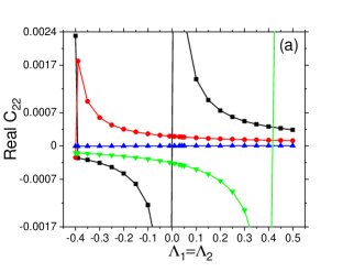
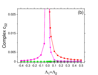
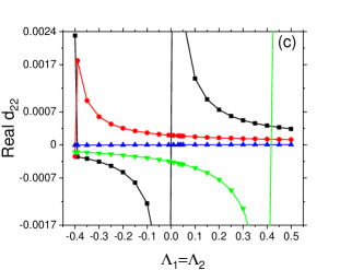
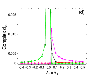
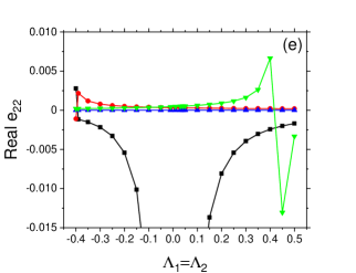
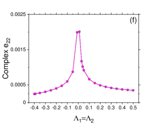
Figure 3: Variation of the coefficients, $c_{22}$, $d_{22}$, and $e_{22}$ as a function of the intra-species interaction parameters. Here, the numbers of bosons are $N_{1}=N_{2}=10000$ and the inter-species interaction parameters $\Lambda_{12}=\Lambda_{21}=0.5$. Eight solutions of coefficients $c_{22}$, $d_{22}$, and $e_{22}$ are shown. Among the eight solutions, four real and four complex-valued solutions are presented in the left and right columns, respectively. Absolute values are plotted in panels (b), (d), and (f). The blue color line in panels (a), (c), and (e) corresponds to the true values of the coefficients by which the coupled-cluster energy is calculated. The rest are discarded for lacking various properties, see the text for further discussion. All the quantities are dimensionless.

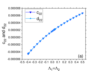
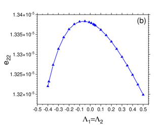
Figure 4: Variation of the true values of the coefficients $c_{22}$, $d_{22}$ and $e_{22}$ as a function of the intra-species interaction parameters. The numbers of bosons are $N_{1}=N_{2}=10000$ and the inter-species interaction parameters $\Lambda_{12}=\Lambda_{21}=0.5$. All the quantities are dimensionless.

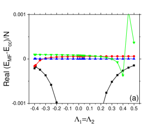
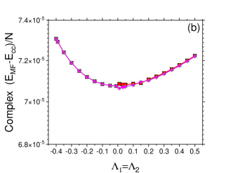
Figure 5: Variation of $(E_{\text{MF}}-E_{\text{cc}})/N$ as a function of the intra-species interaction parameters. The numbers of bosons are $N_{1}=N_{2}=10000$ and the inter-species interaction parameters $\Lambda_{12}=\Lambda_{21}=0.5$. The eight solutions of the energy are shown. The corresponding coefficients are presented in Fig. 3. Among the eight solutions, four real and four complex-valued solutions are presented in panels (a) and (b), respectively. See the text for further details of the determination of the true solutions [marked by blue triangles in panel (a)]. All the quantities are dimensionless.

References

• [1] E. Timmermans, Phase Separation of Bose-Einstein Condensates. Phys. Rev. Lett. 81, 5718 (1998).
• [2] A. R. Sakhel, J. L. DuBois, and H. R. Glyde, Condensate depletion in two-species Bose gases: A variational quantum Monte Carlo study. Phys. Rev. A 77, 043627 (2008).
• [3] S. Zöllner, H. D. Meyer, and P. Schmelcher, Composite fermionization of one-dimensional Bose-Bose mixtures. Phys. Rev. A 78, 013629 (2008).
• [4] M. D. Girardeau, Pairing, Off-Diagonal Long-Range Order, and Quantum Phase Transition in Strongly Attracting Ultracold Bose Gas Mixtures in Tight Waveguides. Phys. Rev. Lett. 102, 245303 (2009).
• [5] K. Anoshkin, Z. Wu, and E. Zaremba, Persistent currents in a bosonic mixture in the ring geometry. Phys. Rev. A 88, 013609 (2013).
• [6] D. S. Petrov, Quantum Mechanical Stabilization of a Collapsing Bose-Bose Mixture. Phys. Rev. Lett. 115, 155302 (2015).
• [7] J. Chen, J. M. Schurer, and P. Schmelcher, Entanglement induced interactions in binary mixtures. Phys. Rev. Lett. 121, 043401 (2018).
• [8] C. Ticknor, Excitations of a trapped two-component Bose-Einstein condensate. Phys. Rev. A 88, 013623 (2013).
• [9] E. Nicklas, W. Muessel, H. Strobel, P. G. Kevrekidis, and M. K. Oberthaler, Nonlinear dressed states at the miscibility-immiscibility threshold. Phys. Rev. A 92, 053614 (2015).
• [10] A. Kleine, C. Kollath, I. P. McCulloch, T. Giamarchi, and U. Schollwöck, Spin-charge separation in two-component Bose gases, Phys. Rev. A 77, 013607 (2008).
• [11] Au-Chen Lee, D. Baillie, and P. B. Blakie, Stability of a flattened dipolar binary condensate: Emergence of the spin roton. Phys. Rev. Research 4, 033153 (2022).
• [12] X. Yu and P. B. Blakie, Propagating Ferrodark Solitons in a Superfluid: Exact Solutions and Anomalous Dynamics. Phys. Rev. Lett. 128, 125301 (2022).
• [13] Joseph C. Smith, D. Baillie, and P. B. Blakie, Quantum Droplet States of a Binary Magnetic Gas. Phys. Rev. Lett. 126, 025302 (2021).
• [14] D. S. Hall, M. R. Matthews, C. E. Wieman, and E. A. Cornell, Measurements of Relative Phase in Two-Component Bose-Einstein Condensates. Phys. Rev. Lett. 81, 1543 (1998).
• [15] D. M. Stamper-Kurn, M. R. Andrews, A. P. Chikkatur, S. Inouye, H. -J. Miesner, J. Stenger, and W. Ketterle, Optical Confinement of a Bose-Einstein Condensate. Phys. Rev. Lett. 80, 2027 (1998).
• [16] S. T. Chui, V. N. Ryzhov, and E. E. Tareyeva, Vortex states in a binary mixture of Bose-Einstein condensates. Phys. Rev. A 63, 023605 (2001).
• [17] G. Thalhammer, G. Barontini, L. De Sarlo, J. Catani, F. Minardi, and M. Inguscio, Double Species Bose-Einstein Condensate with Tunable Interspecies Interactions. Phys. Rev. Lett 100, 210402 (2008).
• [18] S. Gautam and D. Angom, Rayleigh-Taylor instability in binary condensates. Phys. Rev. A 81, 053616 (2010).
• [19] D. J. McCarron, H. W. Cho, D. L. Jenkin, M. P. Köppinger, and S. L. Cornish, Dual-species Bose-Einstein condensate of 87Rb and 133Cs. Phys. Rev. A 84, 011603 (2011).
• [20] L. Wacker, N. B. Jørgensen, D. Birkmose, R. Horchani, W. Ertmer, C. Klempt, N. Winter, J. Sherson, and J. J. Arlt, Tunable dual-species Bose-Einstein condensates of 39K and 87Rb. Phys. Rev. A 92, 053602 (2015).
• [21] A. Bhowmik, P. K. Mondal, S. Majumder, and B. Deb, Density profiles of two-component Bose–Einstein condensates interacting with a Laguerre–Gaussian beam. J. Phys. B: At. Mol. Opt. Phys. 51, 135003 (2018).
• [22] A. Trautmann, P. Ilzhöfer, G. Durastante, C. Politi, M. Sohmen, M. J. Mark, and F. Ferlaino, Dipolar Quantum Mixtures of Erbium and Dysprosium Atoms. Phys. Rev. Lett. 121, 213601 (2018).
• [23] R. Bai, D. Gaur, H. Sable, S. Bandyopadhyay, K. Suthar, and D. Angom, Segregated quantum phases of dipolar bosonic mixtures in two-dimensional optical lattices. Phys. Rev. A 102, 043309 (2020).
• [24] O. E. Alon, Solvable Model of a Generic Driven Mixture of Trapped Bose–Einstein Condensates and Properties of a Many-Boson Floquet State at the Limit of an Infinite Number of Particles. Entropy 22, 1342 (2020).
• [25] R. N. Bisset, L. A. Peña Ardila, and L. Santos, Quantum Droplets of Dipolar Mixtures. Phys. Rev. Lett. 126, 025301 (2021).
• [26] O. E. Alon, Solvable model of a generic trapped mixture of interacting bosons: reduced density matrices and proof of Bose–Einstein condensation. J. Phys. A: Math. Theor. 50, 295002 (2017).
• [27] K. Dželalija, V. Cikojević, J. Boronat, and L. Vranješ Markić, Trapped Bose-Bose mixtures at finite temperature: A quantum Monte Carlo approach. Phys. Rev. A 102, 063304 (2020).
• [28] V. Cikojević, L. V. Markić and J. Boronat, Harmonically trapped Bose–Bose mixtures: a quantum Monte Carlo study. New J. Phys. 20, 085002 (2018).
• [29] M. Lewenstein, A. Sanpera, and V. Ahufinger, Ultracold Atoms in Optical Lattices: Simulating Quantum Many-Body Systems (Oxford University Press, Oxford, UK, 2012).
• [30] I. Morera, G. E. Astrakharchik, A. Polls, and B. Juliá-Díaz, Quantum droplets of bosonic mixtures in a one-dimensional optical lattice. Phys. Rev. Research 2, 022008(R) (2020).
• [31] C. Lévêque and L. B. Madsen, Multispecies time-dependent restricted-active-space self-consistent-field theory for ultracold atomic and molecular gases. J. Phys. B: At. Mol. Opt. Phys. 51 155302 (2018).
• [32] O. E. Alon, A. I. Streltsov, and L. S. Cederbaum, Multiconfigurational time-dependent Hartree method for mixtures consisting of two types of identical particles. Phys. Rev. A 76, 062501 (2007).
• [33] L. Cao, S. Krönke, O. Vendrell, and P. Schmelcher, The multi-layer multi-configuration time-dependent Hartree method for bosons: Theory, implementation, and applications. J. Chem. Phys. 139 134103 (2013).
• [34] L. Cao, V. Bolsinger, S. I. Mistakidis, G. M. Koutentakis, S. Krönke, J. M. Schurer, and P. Schmelcher, A unified ab initio approach to the correlated quantum dynamics of ultracold fermionic and bosonic mixtures. J. Chem. Phys. 147, 044106 (2017).
• [35] U. Manthe and T. Weike, On the multi-layer multi-configurational time-dependent Hartree approach for bosons and fermions. J. Chem. Phys. 146, 064117 (2017).
• [36] J. Paldus and J. Čížek, Time-Independent Diagrammatic Approach to Perturbation Theory of Fermion Systems. Adv. Quantum Chem. 9, 105 (1975).
• [37] J. Čížek, On the Correlation Problem in Atomic and Molecular Systems. Calculation of Wavefunction Components in Ursell‐Type Expansion Using Quantum‐Field Theoretical Methods. J. Chem. Phys. 45, 4256 (1966).
• [38] I. Lindgren and J. Morrison, 1985 Atomic Many-body Theory ed G. E. Lambropoulos and H. Walther (3rd edition, Berlin: Springer) 3 Theory (John Wiley & Sons, Chichester, UK, 2000)
• [39] R. J. Bartlett and M. Musiał, Coupled-Cluster Theory in Quantum Chemistry, Rev. Mod. Phys. 79, 291 (2007).
• [40] R. F. Bishop, U. Kaldor, H. Kümmel, and D. Mukherjee, The Coupled Cluster Approach to Quantum Many-particle Systems, Springer, Heidelberg, 2003.
• [41] Recent Progress in Coupled Cluster Methods: Theory and Applications, edited by P. C. Josef and P. Pittner (Springer, New York, 2010).
• [42] A. F. White and G. Kin-Lic Chan, A Time-Dependent Formulation of Coupled-Cluster Theory for Many-Fermion Systems at Finite Temperature. Journal of Chemical Theory and Computation 14, 5690 (2018).
• [43] H. S. Nataraj, B. K. Sahoo, B. P. Das, and D. Mukherjee, Intrinsic Electric Dipole Moments of Paramagnetic Atoms: Rubidium and Cesium. Phys. Rev. Lett. 101, 033002 (2008).
• [44] A. Bhowmik, N. N. Dutta, and S. Majumder, Vector polarizability of an atomic state induced by a linearly polarized vortex beam: External control of magic, tune-out wavelengths, and heteronuclear spin oscillations. Phys. Rev. A 102, 063116 (2020).
• [45] A. Chakraborty, S. K. Rithvik, and B. K. Sahoo, Relativistic normal coupled-cluster theory analysis of second- and third-order electric polarizabilities of Zn I. Phys. Rev. A 105, 062815 (2022).
• [46] A. Bhowmik, S. Roy, N. N. Dutta and S. Majumder, Study of coupled-cluster correlations on electromagnetic transitions and hyperfine structure constants of W VI. J. Phys. B: At. Mol. Opt. Phys. 50, 125005 (2017).
• [47] L. S. Cederbaum, O. E. Alon, and A. I. Streltsov, Coupled-cluster theory for systems of bosons in external traps. Phys. Rev. A 73, 043609 (2006).
• [48] A. F. White, Y. Gao, A. J. Minnich, and G. Kin-Lic Chan, A coupled cluster framework for electrons and phonons. J. Chem. Phys. 153, 224112 (2020).
• [49] U. Mordovina, C. Bungey, H. Appel, P. J. Knowles, A. Rubio, and F. R. Manby, Polaritonic coupled-cluster theory. Phys. Rev. Research 2, 023262 (2020).
• [50] T. S. Haugland, E. Ronca, E. F. Kjønstad, A. Rubio, and H. Koch, Coupled Cluster Theory for Molecular Polaritons: Changing Ground and Excited States. Phys. Rev. X 10, 041043 (2020).
• [51] B. H. Ellis, S. Aggarwal, and A. Chakraborty, Development of the Multicomponent Coupled-Cluster Theory for Investigation of Multiexcitonic Interactions. J. Chem. Theory Comput. 12, 188 (2016).
• [52] L. S. Cederbaum, A. I. Streltsov, Best mean-field for condensates. Physics Letters A 318, 564 (2003).
• [53] O. E. Alon, A. I. Streltsov, and L. S. Cederbaum, Demixing of Bosonic Mixtures in Optical Lattices from Macroscopic to Microscopic Scales. Phys. Rev. Lett. 97, 230403 (2006).
• [54] A. U. J. Lode, K. Sakmann, O. E. Alon, L. S. Cederbaum, and A. I. Streltsov, Numerically exact quantum dynamics of bosons with time-dependent interactions of harmonic type. Phys. Rev. A 86, 063606 (2012).
• [55] E. Fasshauer and A. U. J. Lode, Multiconfigurational time-dependent Hartree method for fermions: Implementation, exactness, and few-fermion tunneling to open space. Phys. Rev. A 93, 033635 (2016).
• [56] A. U. J. Lode, C. Lévêque, L. B. Madsen, A. I. Streltsov, and O. E. Alon, Colloquium: Multiconfigurational time-dependent Hartree approaches for indistinguishable particles. Rev. Mod. Phys. 92, 011001 (2020).
• [57] S. Klaiman, A. I. Streltsov, and O. E. Alon, Solvable model of a trapped mixture of Bose–Einstein condensates. Chem. Phys. 482, 362 (2017).
• [58] P. A. Bouvrie, A. P. Majtey, M. C. Tichy, J. S. Dehesa, and A. R. Plastino, Entanglement and the Born-Oppenheimer approximation in an exactly solvable quantum many-body system. Eur. Phys. J. D 68, 346 (2014).
• [59] O. E. Alon and L. S. Cederbaum, Effects Beyond Center-of-Mass Separability in a Trapped Bosonic Mixture: Exact Results. J. Phys.: Conf. Ser. 2249, 012011 (2022).
• [60] T. Haugset and H. Haugerud, Exact diagonalization of the Hamiltonian for trapped interacting bosons in lower dimensions. Phys. Rev. A 57, 3809 (1998).
• [61] D. A. Matthews, Accelerating the convergence of higher-order coupled-cluster methods II: coupled-cluster $\Lambda$ equations and dynamic damping. Molecular Physics 118, 19 (2020).
• [62] C. Huber and T. Klamroth, Explicitly time-dependent coupled cluster singles doubles calculations of laser-driven many-electron dynamics. J. Chem. Phys. 134, 054113 (2011).
• [63] B. S. Ofstad, E. Aurbakken, Ø. S. Schøyen, H. E. Kristiansen, S. Kvaal, and T. B. Pedersen, Time-dependent coupled-cluster theory. WIREs Comput. Mol. Sci., e1666 (2023).