Measurements of the neutron timelike electromagnetic form factor with the SND detector

Abstract

The results of the measurement of the $e^{+}e^{-}\to n\bar{n}$ cross section and effective neutron timelike form factor are presented. The data taking was carried out in 2020–2021 at the VEPP-2000 $e^{+}e^{-}$ collider in the center-of-mass energy range from 1891 to 2007 MeV. The general purpose nonmagnetic detector SND is used to detect neutron-antineutrons events. The selection of $n\bar{n}$ events is performed using the time-of-flight technique. The measured cross section is 0.4–0.6 nb. The neutron form factor in the energy range under study varies from 0.3 to 0.2.

Introduction

The internal structure of nucleons is described by electromagnetic formfactors. In the timelike region they are measured using the process of $e^{+}e^{-}$ annihilation to nucleon-antinucleon pairs. The $e^{+}e^{-}\to n\bar{n}$ cross section depends on two formfactors - electric $G_{E}$ and magnetic $G_{M}$ :

$$\frac{d\sigma}{d\Omega} = \frac{\alpha^{2}\beta}{4s}\bigg{[}|G_{M}(s)|^{2}(1+\cos^{2}\theta)$$ (1)

$$+ \frac{1}{\gamma^{2}}|G_{E}(s)|^{2}\sin^{2}\theta\bigg{]}$$

where $\alpha$ is the fine structure constant, $s=4E_{b}^{2}=E^{2}$, where $E_{b}$ is the beam energy and $E$ is the center-of-mass (c.m.) energy, $\beta=\sqrt{1-4m_{n}^{2}/s}$, $\gamma=E_{b}/m_{n}$, $m_{n}$ is the neutron mass and $\theta$ is the antineutron production polar angle. The total cross section has the following form:

$$\sigma(s)=\frac{4\pi\alpha^{2}\beta}{3s}(1+\frac{1}{2\gamma^{2}})|F(s)|^{2},$$ (2)

where the effective form factor $F(s)$ is introduced:

$$|F(s)|^{2}=\frac{2\gamma^{2}|G_{M}(s)|^{2}+|G_{E}(s)|^{2}}{2\gamma^{2}+1}.$$ (3)

The $|G_{E}/G_{M}|$ ratio can be extracted from the analysis of the measured $\cos\theta$ distribution in Eq. (1). At the threshold $|G_{E}|=|G_{M}|$.

The latest results on the neutron form factor near the threshold were obtained in experiments at the VEPP-2000 $e^{+}e^{-}$ collider with the SND detector  SNND . The same work provides a list of previous measurements. At the energy above 2 GeV new data have been obtained by the BESIII  BES . In this work the recent SND results on the $e^{+}e^{-}\to n\bar{n}$ cross section and the neutron timelike formfactor with 4 times higher integrated luminosity than in previous measurement  SNND , are presented.

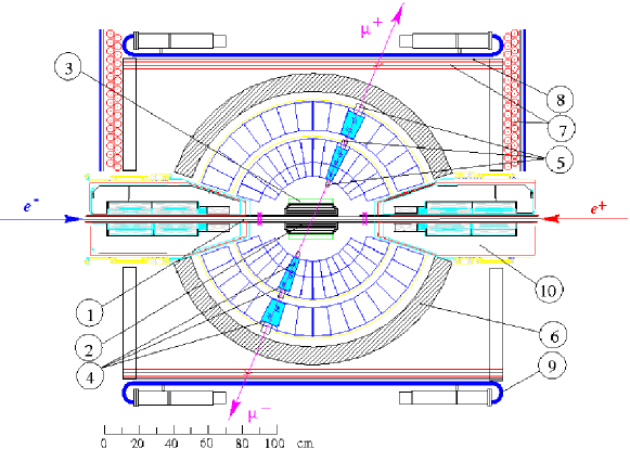
Figure 1: SND detector, section along the beams: (1) beam pipe, (2) tracking system, (3) aerogel Cherenkov counters, (4) NaI (Tl) crystals, (5) vacuum phototriodes, (6) iron absorber, (7) proportional tubes, (8) iron absorber, (9) scintillation counters, (10) VEPP-2000 focusing solenoids.

I Collider, detector, experiment

VEPP-2000 is $e^{+}e^{-}$ collider VEPP2k operating in the energy range from the hadron threshold ($E$=280 MeV) up to 2 GeV. The collider luminosity above the nucleon threshold at 1.87 GeV is of order of $5\times 10^{31}$ cm^-2s^-1. There are two collider detectors at VEPP-2000: SND and CMD-3.

SND (Spherical Neutral Detector)  SNDet1 is a non-magnetic detector, including a tracking system, a spherical NaI(Tl) electromagnetic calorimeter (EMC) and a muon detector (Fig.1). The EMC is the main part of the SND used in the $n\bar{n}$ analysis. The thickness of EMC is 34.7 cm (13.4 radiation length). The antineutron annihilation length in NaI(Tl) varies with energy from several cm close to the $n\bar{n}$ threshold to $\sim$15 cm at the maximum available energy  Annih , so nearly all produced antineutrons are absorbed in the detector.

The EMC is used to measure the event arrival time. Starting from 2019 a system of flash ADC modules  Timr , measuring the signal waveform, is installed on each of the 1640 EMC counters. When fitting the flash ADC output waveform, the time and amplitude of the signal in the counters are calculated. The event time is calculated as the energy weighted average time. The time resolution obtained with $e^{+}e^{-}\to\gamma\gamma$ events is about 0.8 ns.

This article presents the analysis results of data with the integrated luminosity of $80$ pb^-1, collected in the energy range $1.89$ - $2.0$ GeV in 8 energy points.

II Selection of $n\bar{n}$ events

Antineutron from the $n\bar{n}$ pair in most cases annihilates, producing pions, nucleons, photons and other particles, which deposit up to 2 GeV in EMC. The neutron from the $n\bar{n}$ pair release a small signal in EMC, which poorly visible against the background of a strong $\bar{n}$ annihilation signal, so it is not taken into account. The $n\bar{n}$ events are reconsructed as multiphoton events.

Main features of $n\bar{n}$ events are absence of charged tracks and photons from the collision region and a strong imbalance in the event momentum. To create the $n\bar{n}$ selection conditions we consider the sources of the background including the cosmic background, the background from $e^{+}e^{-}$ annihilation processes and from the electron and positron beams in the collider.

Based on these specific features of the $e^{+}e^{-}\to n\bar{n}$ process, selection conditions were divided into three groups.

In the first group the conditions are collected that suppress the background from the $e^{+}e^{-}$ annihilation events. These include the condition of no charged tracks in an event, the limit on the total event momentum (p/2$E_{b}>$0.4), and a limitation on the transverse shower profile in EMC  xi2gam , which must be wider than that from the photons from the collision region.

In the second group the selection conditions should suppress the cosmic background. Here the veto of muon system is included and special conditions, analyzing the energy deposition shape in EMC and removing cosmic events passing through the muon veto  SNND . Basically, these are cosmic showers in EMC.

The third group of selection cuts contains the restriction on the total energy deposition in EMC — $E_{dep}>E_{b}$. Such a restriction almost completely suppresses the beam background, although the detection efficiency also decreases by about 20%.

The listed selection conditions are similar to those described in our recent work  SNND . The only difference is that there is no limitation on the energy in the EMC third layer. This slightly increased the detection efficiency, although it did increase the cosmic background. After imposing the described selection conditions, we have about 400 events/$pb$ left for further analysis.

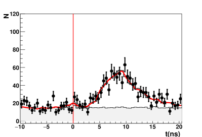
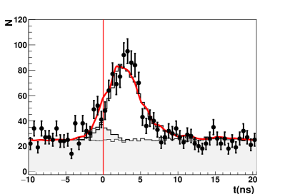
Figure 2: The time distribution of selected data events (points with error bars) at $E_{b}=945$ MeV (left panel) and at $E_{b}=980$ MeV (right panel). The position $t=0$ corresponds to the moment of beams collision. The wide peak to the right is the contribution of $n\bar{n}$ events. The light-shaded histogram shows the cosmic background (uniform in time) and beam background (peak at $t=0$). The solid line is the result of the fit.

III Getting the number of $n\bar{n}$ events

The time spectra for selected data events are shown in Fig. 2. Zero time corresponds to events in the moment of beam collision. Three main components are distinguished in the time spectrum in the figures shown: a beam background at t=0, a cosmic background uniform in time, and a delayed signal from $n\bar{n}$ events, wide in time. Respectively, the measured time spectra are fitted by the sum of these three components in the following form :

$$F(t)=N_{n\bar{n}}H_{n\bar{n}}(t)+N_{\rm csm}H_{\rm csm}(t)+N_{\rm bkg}H_{\rm bkg}(t),$$ (4)

where $H_{n\bar{n}}$, $H_{\rm csm}$ and $H_{\rm bkg}$ are normalized histograms, describing time spectra for the $n\bar{n}$ signal, cosmic and beam + physical background, respectively. $N_{n\bar{n}}$, $N_{\rm csm}$, and $N_{\rm bkg}$ are the corresponding event numbers, obtained from the fit. The shape of the beam+physical background time spectrum $H_{\rm bkg}$ is measured at the energies below the $n\bar{n}$ threshold. The cosmic time spectrum $H_{\rm csm}$ is measured with the lower EMC threshold $0.9\cdot E_{b}$ in coincidence with the muon system signal. The $H_{n\bar{n}}$ spectrum is calculated by the MC simulation the $e^{+}e^{-}\to n\bar{n}$ process.

Comparison of time spectra in data and MC gives a wider data time distribution for both $e^{+}e^{-}\to\gamma\gamma$ and $e^{+}e^{-}\to n\bar{n}$ events. For the $e^{+}e^{-}\to\gamma\gamma$ this is due to the finite time resolution of our timing system  Timr , which is not adequately simulated. So we convolve the MC time spectrum with a Gaussian with $\sigma_{\gamma\gamma}=$ 0.8 ns. For $e^{+}e^{-}\to n\bar{n}$ events the covolution is done with $\sigma_{nn}=1.5$–2 ns depending on the energy.

Moreover, in addition to the above, we correct the MC ${n\bar{n}}$ time spectrum, since the shape of MC time spectrum $H_{n\bar{n}}$ does not describe data well. This discrepancy is explained by the incorrect relationship between the processes of antineutron annihilation and scattering in MC, as well as by the incorrect description of the annihilation products. To modify the MC time spectrum, separate MC time spectra were plotted for the cases of the first $\bar{n}$ interaction of scattering ($H_{n\bar{n}}^{s}$) and annihilation ($H_{n\bar{n}}^{a}$). The share of annihilation events in MC was about 33%. The annihilation gives the time spectrum close to the exponential while the scattering has delayed and more wide time spectrum with the non exponential shape. The $H_{n\bar{n}}$ spectrum (Eq.4) was taken in fit as a linear sum of two spectra described above: $H_{n\bar{n}}=\alpha H_{n\bar{n}}^{a}+(1-\alpha)H_{n\bar{n}}^{s}$ . The value $\alpha$ (the share of annihilation events) was the fit parameter. As a result of the fit this parameter turned out to be greater than in MC – $\simeq$60% and accordingly the proportion of scattering fell to $\simeq$40%. As can be seen in Fig.2, the modified MC time spectrum describes the data well.

The visible cross section $\sigma_{bg}$ of the beam+physical background, obtained during fitting, is about 7 pb and does not significantly depend on the beam energy. The main contribution into $\sigma_{bg}$ comes from the processes with neutral kaons in the final state: $e^{+}e^{-}\to K_{S}K_{L}\pi^{0}$, $K_{S}K_{L}\eta$ and similar other. The measured residual cosmic background rate has the intensity $\sim$0.01 Hz, which corresponds to the suppression of the number of cosmic events, that have pass the hardware selection in the detector electronics, approximately by $2\times 10^{4}$ times.

Table 1: The beam energy ($E_{b}$), integrated luminosity ($L$), number of selected $n\bar{n}$ events ($N_{n\bar{n}}$), the factor taking into account radiative corrections and energy spread ($1+\delta$), corrected detection efficiency ($\varepsilon$), measured $e^{+}e^{-}\to n\bar{n}$ cross section $\sigma$, and neutron effective form factor ($F_{n}$). The quoted errors for $N$, $\sigma$ are statistical and systematic. For the detection efficiency, the systematic uncertainty is quoted. For $F_{n}$, the combined statistical and systematic uncertainty is listed.

N	$E_{b}$(MeV)	$L$(pb)	$N_{n\bar{n}}$	$1+\delta$	$\varepsilon$	$\sigma$(nb)	$F_{n}$
1	945.5	8.54	$676\pm 37$	0.746	$0.253\pm 0.021$	$0.420\pm 0.023\pm 0.036$	$0.322\pm 0.016$
2	950.3	8.86	$834\pm 37$	0.787	$0.246\pm 0.015$	$0.485\pm 0.022\pm 0.031$	$0.301\pm 0.012$
3	960.3	8.33	$767\pm 35$	0.840	$0.217\pm 0.013$	$0.506\pm 0.023\pm 0.032$	$0.266\pm 0.010$
4	970.8	8.07	$718\pm 34$	0.870	$0.229\pm 0.017$	$0.447\pm 0.021\pm 0.034$	$0.230\pm 0.011$
5	968.8	5.51	$524\pm 34$	0.870	$0.186\pm 0.020$	$0.589\pm 0.039\pm 0.065$	$0.267\pm 0.017$
6	980.3	7.70	$654\pm 37$	0.900	$0.216\pm 0.018$	$0.436\pm 0.025\pm 0.038$	$0.216\pm 0.011$
7	990.4	8.77	$624\pm 38$	0.920	$0.183\pm 0.019$	$0.422\pm 0.026\pm 0.045$	$0.204\pm 0.013$
8	1003.5	20.06	$1075\pm 50$	0.947	$0.151\pm 0.014$	$0.374\pm 0.018\pm 0.035$	$0.186\pm 0.010$

The numbers of found $n\bar{n}$ events are listed in the Table 1 with the total number close to 6000. The Table shows only statistical errors of the fitting. A source of systematic error in the $n\bar{n}$ event number can be uncertainties in the magnitide and shape of the time spectrum of the beam and cosmic background. The error introduced by these sources is 15 events at $E_{b}$=1000 MeV and less than 8 events at lower energies. These values are much lower than statitistical errors in the Table 1 and are not taken into account in what follows.

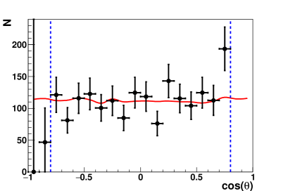
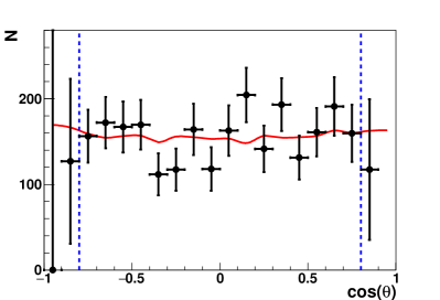
Figure 3: The antineutron $\cos\theta_{a}$ distribution for data (points with error bars) and MC (horizontal line) at $E_{b}=970$ MeV (left panel) and $E_{b}=1000$ MeV (right panel). Dotted vertical lines correspond to the polar angle cutoff.

Figure 4: The corrected detection efficiency versus energy.

Figure 5: The MC detection efficiency as a function of antineutron $\cos{\theta}$ at $E_{b}$=960 MeV. Dotted vertical lines correspond to the polar angle cutoff.

IV Antineutron angular distribution

The antineutron production angle $\theta_{n}$ is determined by the direction of the event momentum with an accuracy of about 5 degrees. Distribution over $\cos\theta_{n}$ for data and MC events is shown in Fig. 3. The MC simulation was done using Eq. (1) with the assumption $G_{E}=G_{M}$. The detection efficiency in the selection interval $36^{\circ}<\theta_{n}<144^{\circ}$ is 80%. It is seen from the Fig. 3 that the data and MC distributions agree well with each other, which confirms the MC angular model. It is also worth noting that the previous measurements of the $|G_{E}/G_{M}|$ value SNND also do not contradict the hypothesis $G_{E}=G_{M}$.

V Detection efficiency

The detection efficiency $\varepsilon$ versus energy under accepted selection conditions (Section II) is shown in Fig. 5. When calculating $\varepsilon$ we used the MC simulation of the $e^{+}e^{-}\to n\bar{n}$ process with the GEANT4 toolkit GEANT4 , version 10.5. In addition, the simulation included the beam energy spread $\sim~{}1$ MeV and the emission of photons by initial electrons and positrons. The simulation also took into account non-operating detector channels as well as overlaps of the beam background with recorded events. To do this, during the experiment, with a pulse generator, synchronized with the moment of beam collision, special superposition events were recorded, which were subsequently superimposed on MC events. The detection efficiency $\varepsilon$ in Fig. 5 is corrected for the difference between the data and MC. This correction is discussed later. Numerical values of the efficiency are given in the Table 1. A decrease of $\varepsilon$ with energy can be explained by the energy dependence of the selection parameters, as well as by an increase in the energy that goes beyond the calorimeter. In Fig. 5 the angular detection efficiency is shown at the beam energy $E_{b}=960$ MeV.

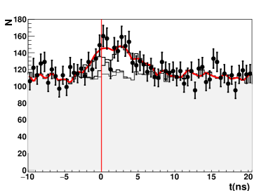
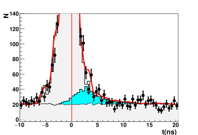
Figure 6: The event time spectra with inverted selection conditions. Left panel — inverted 2-nd group cut at $E_{b}=970$ MeV, Right panel — inverted 3-d group cut with $0.7E_{b}<E_{\rm cal}<E_{b}$ at $E_{b}=960$ MeV. Light shaded histogram shows the background distribution. Dark shaded histogram in the right plot is $n\bar{n}$ contribution.

The detection efficiency in our measurement is of order of 20%. It is important to find out how correctly the proportion of events outside the selection condition is simulated. Corrections were calculated fot three groups of selection conditions described in chapter II. To do this, we invert the selection conditions for each selection group and then calculate the corresponding corrections $\delta$ for detection efficiency in each of 8 energy points as follows:

$$\delta=\frac{n_{0}}{n_{0}+n_{1}}\frac{m_{0}+m_{1}}{m_{0}},$$ (5)

where $n_{0}$ ($n_{1}$) is the number of $n\bar{n}$ events determined with standard (inverted) selection cuts. These numbers were calculated during the time spectra fitting with the Eq.4, as it is described in the chapter III. The values $m_{0}$ and $m_{1}$ refer respectively to the MC simulation event numbers. Examples of the time spectra obtained with inverted conditions are shown in Fig. 6.

Table 2: The beam energy ($E_{b}$), the correction to the detection efficiency $\delta_{1}$ from SND internal system, the correction $\delta_{2}$ from SND external system, the correction $\delta_{3}$ from the EMC thresholds, the correction $\delta_{E}$ from the lost EMC energy, the correction $\delta_{t}$ is the total correction.

	$E_{b}$ (MeV)	$\delta_{1}$	$\delta_{2}$	$\delta_{3}$	$\delta_{E}$	$\delta_{t}$
1	945.5	$0.991\pm 0.022$	$1.292\pm 0.092$	$0.971\pm 0.038$	$1.005\pm 0.005$	$1.249\pm 0.102$
2	950.3	$0.977\pm 0.018$	$1.214\pm 0.062$	$0.985\pm 0.030$	$1.009\pm 0.009$	$1.179\pm 0.072$
3	960.3	$9.966\pm 0.019$	$1.077\pm 0.050$	$0.992\pm 0.028$	$1.012\pm 0.012$	$1.044\pm 0.062$
4	970.8	$0.949\pm 0.021$	$1.198\pm 0.061$	$0.980\pm 0.050$	$1.018\pm 0.018$	$1.134\pm 0.084$
5	968.8	$0.958\pm 0.027$	$1.031\pm 0.080$	$0.896\pm 0.044$	$1.018\pm 0.018$	$0.901\pm 0.097$
6	980.3	$0.997\pm 0.031$	$1.102\pm 0.073$	$0.986\pm 0.043$	$1.021\pm 0.021$	$1.106\pm 0.093$
7	990.4	$0.925\pm 0.033$	$1.131\pm 0.080$	$0.889\pm 0.041$	$1.024\pm 0.024$	$0.952\pm 0.099$
8	1003.5	$0.915\pm 0.024$	$1.065\pm 0.056$	$0.796\pm 0.028$	$1.028\pm 0.028$	$0.797\pm 0.073$

The first group of selection conditions includes the requirement of no charged tracks in an event. When studying inverse selections we assume the presence of central charged tracks with $D_{xy}>0.5$ cm, where $D_{xy}$ is the distance between the track and the axis of the beams. A possible background from the related process $e^{+}e^{-}\to p\bar{p}$ should be discussed here. In the energy region $E_{b}>960$ MeV protons and antiproptons give central collinear tracks and rejected by the requirement $D_{xy}>0.5$ cm, as well as events of other processes of $e^{+}e^{-}$ annihilation with charged tracks. However at $E_{b}<960$ MeV the protons and antiproptons are slow and stop at the collider vacuum pipe. In this case the antiproton annihilates with the production of charged tracks, wchich can be with $D_{xy}>0.5$ cm. But here, too, the $e^{+}e^{-}\to p\bar{p}$ background is suppressed by the fitting of time spectrum, since the annihilation delay time does not exceed 1 ns. For the second group the inverted selection conditions were used without changes. For the third group of selection conditions, a partial inversion was used, that is, the condition $0.7E_{b}<E_{\rm cal}<E_{b}$ was applied.

An additional correction arises from the events, in which the antineutrons pass the calorimeter without interaction, and from the events with a small calorimeter energy $E_{\rm cal}<0.7E_{b}$. These events are not taken into analysis due to the large background and therefore not available for correction with the procedure described above. Their share in MC varies from 1.9% at the energy $E_{b}$=945 MeV to 8.5% at $E_{b}$=1000 MeV. It was previously noted in chapter  III, that to desribe the shape of data time spectrum the contribution of the process of antineutron scattering in MC should be reduced by a factor of 1.5. With such a change, the proportion of events with $E_{\rm cal}<0.7E_{b}$ in MC reduces to 1.4% at $E_{b}$=945 to 5.7% at $E_{b}$=1000 MeV. The difference between these values is taken into account as an additional correction $\delta_{E}$ to the detection efficiency with the 100% of uncertainty.

The measured by selection groups corrections $\delta_{1},\delta_{2},\delta_{3}$, as well as $\delta_{E}$, are multiplied $\delta_{t}=\delta_{1}\delta_{2}\delta_{3}\delta_{E}$ and all are given in the Table 2. It can be seen, that the total efficiency correction $\delta_{t}$ changes in limits 0.8—1.25 with energy, what is explained by the strong energy dependence of the antineutron absobtion length.

The corrected detection efficiency is obtained from the MC efficiency by multiplying by the total correction $\delta_{t}$. The values of the corrected efficiency are given along with systematic errors in the Table 1. Here, unlke our previous measurement SNND , the corrections in different energy points are not correlated.

VI The measured $e^{+}e^{-}\to n\bar{n}$ cross section

Figure 7: The $e^{+}e^{-}\to n\bar{n}$ cross section measured in this work in comparison with previous SND measurement SNND and BESIII BES data. The solid curve is the fit result. Only new SND and BESIII data were used in the fit.

Figure 8: The measured neutron timelike formfactor (solid black points) compared with BESIII BES (red stars) and BABAR Babar proton formfactor (blue empty squares) The solid line is the polinomial fit, described in the text.

Using the number of $n\bar{n}$ events $N_{n\bar{n}}$ , luminosity $L$ and detection efficiency $\varepsilon$ (Table 1), the visible cross section $\sigma_{vis}(E)=N_{n\bar{n}}/L\varepsilon$ can be calculated. The Born cross section $\sigma(E)$ we need is related to the visible cross $\sigma_{vis}(E)$ in the following form :

$$\sigma_{vis}(E) = \sigma(E)(1+\delta(E))$$ (6)

$$= \int_{-\infty}^{+\infty}G(E^{\prime},E)dE^{\prime}$$

$$\int_{0}^{x_{max}}W(s,x)\sigma(s(1-x))dx,$$

where $W(s,x)$ is the radiator function Radcor describing emission of photons with energy $xE_{b}$ by initial electrons and positrons, $G(E^{\prime},E)$ is a Gaussian function describing the c.m. energy spread. In function $W(s,x)$ the contribution of the vacuum polarization is not taken into account, so our Born cross section is a “dressed” cross section. The factor $(1+\delta(E))$ takes into account both the radiative corrections and beam energy spread. This factor is calculated in each of 8 energy points using the Born cross section, obtained by the fitting of the visible cross section using Eq. 6. The energy dependence of the Born cross section is described by Eq.2, in which the neutron effective formfactor has a form of a second order polinomial function, as shown in more detail in the next chapter.

The measured Born cross section is shown in the Fig. 8 and listed in the Table 1. The dominant contribution into systematic error is made by the detection efficiency correction error, given in the Table 2. Uncertainties in the value of luminosity (1%) and radiative correction (2%) are also taken into account. In Fig. 8 the total statistical and systematic error is shown. In comparison with our preceding work  SNND , the measured cross section has 2 times lower statistical error and 1.5 times lower systematic error. At the maximum energy $E=2$ GeV our cross section is in good agreement with the last BESIII measurement BES .

VII The neutron effective timelike formfactor

The effective neutron form factor calculated from the measured cross section using Eq. (2) is listed in the Table 1 and shown in Fig. 8 as a function of the antineutron momentum together with the BESIII data BES and the proton effective form factor measured by the BABAR experiment Babar . The curve in Fig. 8, approximating the form factor, is a second order polinimial $|F_{n}|=a_{0}+a_{1}p_{n}+a_{2}p_{n}^{2}$, in which the parameters $a_{i}$ are obtained during fitting and $p_{n}$ is the antineutron momentum. The following parameters values are obtained: $a_{0}=0.398\pm 0.022$, $a_{1}=-0.713\pm 0.126$, $a_{2}=0.268\pm 0.166$. When the fitting curve continues to zero momentum, the expected value of the neutron formfactor at the threshold will be $a_{0}\simeq$0.4. One can see from the Fig. 8, that the proton formfactor noticably larger that the neutron one and their ratio near the threshold could be close to $3/2$.

VIII Summary

The experiment to measure the $e^{+}e^{-}\to n\bar{n}$ cross section and the neutron timelike form factor has been carried out with the SND detector at the VEPP-2000 $e^{+}e^{-}$ collider in the energy region from 1891 to 2007 MeV. The measured $e^{+}e^{-}\to n\bar{n}$ cross varies with energy within 0.4$\div$0.6 nb and agrees with recent SND measurement SND SNND , however has 2 times better statistical accuracy. At the maximum energy our cross section is in agreement with the last BESIII measurement BES . The neutron effective timelike form factor is extracted from the measured cross section using Eq.2. Form factor decreases with energy from 0.3 to 0.2. In the value, the neutron form factor turns out to be noticeably less than the proton one.

ACKNOWLEDGMENTS. This work was carried out on the RSF fund grant No. 23-22-00011.

References

- (1) M. N. Achasov et al. (SND Collaboration), Eur. Phys. J. C (2022:82:761). http://doi.org/10.1140/epjc/s10052-022-10696-0
- (2) M. Ablikim et al. (BESIII Collaboration), Nat. Phys. 17, 1200 (2021). https://doi.org/10.1038/s41567-021-01345-6
- (3) P. Yu. Shatunov et al., Part. Nucl. Lett. 13, 995 (2016). http://dx.doi.org/10.1134/S154747711607044X
- (4) M. N. Achasov et al. (SND Collaboration), Nucl. Instrum. Meth. A 449, 125 (2000). http://dx.doi.org/10.1016/S0168-9002(99)01302-9
- (5) M. Astrua et al., Nucl. Phys. A 697, 209 (2002). http://dx.doi.org/10.1016/S0375-9474(01)01252-0
- (6) M. N. Achasov et al., JINST 10, T06002 (2015). http://dx.doi.org/10.1088/1748-0221/10/06/T06002
- (7) A. V. Bozhenok et al., Nucl. Instr. Meth. A 379, 507 (1996). http://dx.doi.org/10.1016/0168-9002(96)00548-7
- (8) J. Allison et al. (GEANT Collaboration), Nucl. Instr. Meth. A 835, 186 (2016). https://doi.org/10.1016/j.nima.2016.06.125, https://geant4-data.web.cern.ch/ReleaseNotes/ReleaseNotes4.10.5.html
- (9) E. A. Kuraev and V. S. Fadin, Sov. J. Nucl. Phys. 41, 466 (1985).
- (10) J. P. Lees et al. (BABAR Collaboration), Phys. Rev. D 87, 092005 (2013). Phys. Rev. D 88, 072009 (2013). http://dx.doi.org/10.1103/PhysRevD.87.092005 http://dx.doi.org/10.1103/PhysRevD.88.072009