HAT: Hybrid Attention Transformer for
Image Restoration

Abstract

Transformer-based methods have shown impressive performance in image restoration tasks, such as image super-resolution and denoising. However, we find that these networks can only utilize a limited spatial range of input information through attribution analysis. This implies that the potential of Transformer is still not fully exploited in existing networks. In order to activate more input pixels for better restoration, we propose a new Hybrid Attention Transformer (HAT). It combines both channel attention and window-based self-attention schemes, thus making use of their complementary advantages. Moreover, to better aggregate the cross-window information, we introduce an overlapping cross-attention module to enhance the interaction between neighboring window features. In the training stage, we additionally adopt a same-task pre-training strategy to further exploit the potential of the model for further improvement. Extensive experiments have demonstrated the effectiveness of the proposed modules. We further scale up the model to show that the performance of the SR task can be greatly improved. Besides, we extend HAT to more image restoration applications, including real-world image super-resolution, Gaussian image denoising and image compression artifacts reduction. Experiments on benchmark and real-world datasets demonstrate that our HAT achieves state-of-the-art performance both quantitatively and qualitatively. Codes and models are publicly available at https://github.com/XPixelGroup/HAT.

1 Introduction

Image restoration (IR) is a classic problem in computer vision. It aims to reconstruct a high-quality (HQ) image from a given low-quality (LQ) input. Classic IR tasks encompass image super-resolution, image denoising, compression artifacts reduction, and etc. Image restoration plays an important role in computer vision and has widespread application in areas such as AI photography [1], surveillance imaging [2], medical imaging [3], and image generation [4]. Since deep learning has been successfully applied to IR tasks [5, 6, 7], numerous methods based on the convolutional neural network (CNN) have been proposed [8, 9, 10, 11, 12, 13] and almost dominate this field in the past few years. Recently, due to the success in natural language processing, Transformer [14] has attracted increasing attention in the computer vision community. After making rapid progress on high-level vision tasks [15, 16, 17], Transformer-based methods are also developed for low-level vision tasks [18, 19, 20, 21, 22]. A sucessful example is SwinIR [22], which obtains a breakthrough improvement on various IR tasks.

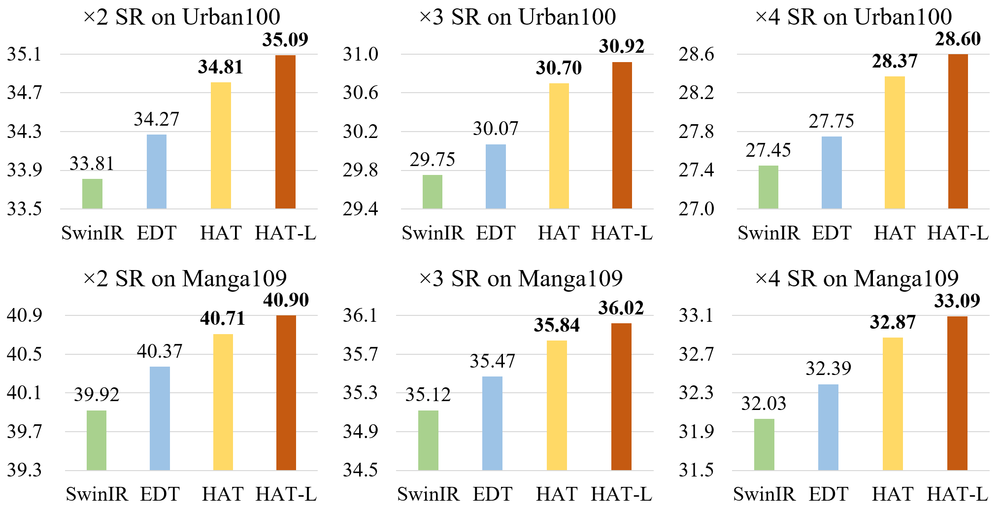
Figure 1: Performance comparison of the proposed HAT with the state-of-the-art methods SwinIR [22] and EDT [21] on image SR. HAT-L represents a larger variant of HAT. Our approach can surpass the state-of-the-art methods by 0.3dB$\sim$1.2dB.

Despite the success, “why Transformer is better than CNN” remains a mystery. An intuitive explanation is that this kind of network can benefit from the self-attention mechanism and utilize long-range information. Thus, we take image super-resolution (SR) as the example and employ the attribution analysis method - Local Attribution Map (LAM) [23] to examine the involved range of utilized information in SwinIR. Interestingly, we find that SwinIR does NOT exploit more input pixels than CNN-based methods (e.g., RCAN [10]). Additionally, although SwinIR obtains higher quantitative performance on average, it produces inferior results to RCAN in some samples, due to the limited range of utilized information. These phenomena illustrate that Transformer has a stronger ability to model local information, but the range of its utilized information needs to be expanded. In addition, we also find that blocking artifacts would appear in the intermediate features of SwinIR. It demonstrates that the shift window mechanism cannot perfectly realize cross-window information interaction.

To address the above-mentioned limitations and further develop the potential of Transformer for IR, we propose a Hybrid Attention Transformer, namely HAT. Our HAT combines channel attention and self-attention schemes, in order to take advantage of the former’s capability in using global information and the powerful representative ability of the latter. Besides, we introduce an overlapping cross-attention module to achieve more direct interaction of adjacent window features. Benefiting from these designs, our model can activate more pixels for reconstruction and thus obtains significant performance improvement.

Since Transformers do not have an inductive bias like CNNs, large-scale data pre-training is important to unlock the potential of such models. In this paper, we provide an effective same-task pre-training strategy. Different from IPT [18] using multiple restoration tasks for pre-training and EDT [21] utilizing multiple degradation levels of a specific task for pre-training, we directly perform pre-training using large-scale dataset on the same task. We believe that large-scale data is what really matters for pre-training. Experimental results show the superiority of our strategy. Equipped with the above designs, HAT can surpass the state-of-the-art methods by a large margin (0.3dB$\sim$1.2dB) on the SR task, as shown in Fig. 1.

Overall, our main contributions are four-fold:

• We design a new Hybrid Attention Transformer (HAT) that combines self-attention, channel attention and a new overlapping cross-attention to activate more pixels for high-quality image restoration.

• We propose an effective same-task pre-training strategy to further exploit the potential of SR Transformer and show the importance of large-scale data pre-training for the SR task.

• Our method significantly outperforms existing state-of-the-art methods on the SR task. By further scaling up HAT to build a big model, we greatly extend the performance upper bound of the SR task.

• Our method also achieves state-of-the-art performance on image denoising and compression artifacts reduction, showing the superiority of our approach on various image restoration tasks.

A preliminary version of this work was presented at CVPR2023 [24]. The present work expands upon the initial version in several significant ways. Firstly, we provide a theoretic illustration of LAM, which can facilitate readers’ understanding of the motivation behind our method and the rationality of its design. Secondly, we investigate a flexible structure of HAT for application to different IR tasks, allowing us to further explore the potential breadth of HAT. Thirdly, we extend our method to real-world image super-resolution based on a high-order degradation model. The promising results demonstrate the potential of HAT for real-world applications. Additionally, we further extend HAT for image denoising and compression artifacts reduction. Extensive experiments show that our method achieves state-of-the-art performance on several IR tasks.

2 Related Work

2.1 Image Super-Resolution

Since SRCNN [5] first introduces deep convolution neural networks (CNNs) to the image SR task and obtains superior performance over conventional SR methods, numerous deep networks [25, 8, 26, 27, 28, 29, 10, 30, 31, 32, 22, 21] have been proposed for SR to further improve the reconstruction quality. For instance, many methods apply more elaborate convolution module designs, such as residual block [33, 28] and dense block [12, 29], to enhance the model representation ability. Several works explore more different frameworks like recursive neural network [34, 35] and graph neural network [36]. To improve perceptual quality, [33, 12, 37, 38] introduce adversarial learning to generate more realistic results. By using attention mechanism, [10, 30, 11, 39, 31, 32] achieve further improvement in terms of reconstruction fidelity. Recently, a series of Transformer-based networks [18, 22, 21] are proposed and constantly refresh the state-of-the-art of SR task, showing the powerful representation ability of Transformer.

To better understand the working mechanisms of SR networks, several works [23, 40, 41, 42, 43] are proposed to analyze and interpret the SR networks. LAM [23] adopts the integral gradient method to explore which input pixels contribute most to the final performance. DDR [40] reveals the deep semantic representations in SR networks based on deep feature dimensionality reduction and visualization. FAIG [41] is proposed to find discriminative filters for specific degradations in blind SR. [42] introduces channel saliency map to demonstrate that Dropout can help prevent co-adapting for real SR networks. SRGA [43] aims to evaluate the generalization ability of SR methods. In this work, we exploit LAM [23] to analyse and understand the behavior of SR networks.

2.2 Vision Transformer

Recently, Transformer [14] has attracted the attention of computer vision community due to its success in the field of natural language processing. A series of Transformer-based methods [15, 44, 45, 17, 16, 46, 47, 48, 49, 50, 51, 52] have been developed for high-level vision tasks, including image classification [16, 15, 44, 53, 54], object detection [55, 56, 16, 57, 48], segmentation [58, 17, 59, 60], etc. Although vision Transformer has shown its superiority on modeling long-range dependency [15, 61], there are still many works demonstrating that the convolution can help Transformer achieve better visual representation [45, 62, 63, 50, 51]. Due to the impressive performance, Transformer has also been introduced for low-level vision tasks [18, 19, 22, 64, 65, 20, 66, 21]. Specifically, IPT [18] develops a ViT-style network and introduces multi-task pre-training for image processing. SwinIR [22] proposes an image restoration Transformer based on [16]. VRT[66] introduces Transformer-based networks to video restoration. EDT[21] adopts self-attention mechanism and multi-related-task pre-training strategy to further refresh the state-of-the-art of SR. However, existing works still cannot fully exploit the potential of Transformer, while our method can activate more input pixels for better reconstruction.

2.3 Deep Networks for Image Restoration

Image restoration aims to generate a high-quality image from a degraded image. Since deep learning was successfully applied to various image restoration tasks such as image super-resolution [25], image denoising [7], and compression artifacts reduction [6], a large number of deep networks have been proposed for image restoration [9, 67, 68, 69, 70, 71, 19, 20, 65, 22, 21, 72]. Before Transformer is applied to low-level vision tasks and demonstrates impressive performance, CNN-based networks dominates this field. For instance, ARCNN [6] stacks several convolution layers to build a deep network for JPEG compression artifacts reduction. DnCNN [7] uses convolution combined with batch normalization to construct an image denoising deep network. RDN [68] introduces a residual dense CNN network for various image restoration tasks. In  [73], dozens of CNN methods for image super-resolution are investigated. As Transformer is widely used in computer vision tasks, Transformer-based image restoration methods are gradually developed. SwinIR [22] is based on Swin Transformer [16] and shows impressive performance on image super-resolution, image denoising and JPEG compression artifacts reduction. Uformer [19] designs a U-style Transformer networks for various image restoration tasks. Restormer [20] constructs a U-style Transformer based on the transposed self-attention and achieves state-of-the-art performance on multiple image restoration tasks. Transformer-based networks have demonstrated superior performance compared to previous CNN-based methods. Moreover, our method introduces hybrid attention mechanism and further improves the performance of image restoration Transformer.

3 Motivation

Swin Transformer [16] has already presented excellent performance on the image SR task [22]. Then we are eager to know what makes it work better than CNN-based methods and what problems it still has. To reveal its working mechanism, we resort to a diagnostic tool - LAM [23], and feature visualization analysis. In this section, we first provide an overview of LAM. Then we conduct LAM and feature visualization analysis for the SR Transformer.

3.1 An overview of LAM

Local Attribution Map (LAM) [23] is an attribution approach based on integrated gradients [74]. Integrated gradients represent the contribution of each pixel in the input image on the final output result. Formally, let $F:\mathbb{R}^{n}\mapsto[0,1]$ be a deep classification network. Let $I\in\mathbb{R}^{n}$ be the input and $I^{\prime}\in\mathbb{R}^{n}$ be the baseline input (e.g. a black image). The integrated gradient along the $i^{th}$ dimension is defined as

$$\mathsf{IntegratedGrads}_{i}(I):=(I_{i}-I^{\prime}_{i})\times\int_{\theta=0}^{1}\tfrac{\partial F(I^{\prime}_{i}+\theta\times(x-I^{\prime}_{i})))}{\partial I_{i}}~{}d\theta.$$ (1)

Let $\lambda(\theta):[0,1]\mapsto\mathbb{R}^{h\times w}$ be a smooth function specifying a path from the baseline $I^{\prime}$ to the input $I$ (i.e., $\lambda(0)=I^{\prime}$ and $\lambda(1)=I$), path integrated gradients along the $i^{th}$ dimension for an input $I$ is defined as

$$\mathsf{PathIntegratedGrads}^{\lambda}_{i}(I):=\int_{0}^{1}\frac{\partial F(\lambda(\theta))}{\partial\lambda_{i}(\theta)}\times\frac{\partial\lambda_{i}(\theta)}{\partial\theta}d\theta,$$ (2)

where $\frac{\partial F(I)}{\partial I_{i}}$ is the gradient along the $i^{th}$ dimension at $I$.

LAM calculates the path integrated gradients map by designing the baseline input $I^{\prime}$ and path function $\lambda$ according to the characteristic of the SR task. Since the SR task focuses more on the reconstruction of textures and edges, LAM selects the blurred version of the LR image as the baseline input, denoted as

$$I^{\prime}=\omega(\sigma)\otimes I,$$ (3)

where $\otimes$ represents convolution operation and $\omega(\sigma)$ is the Gaussian blur kernel parameterized by the kernel width $\sigma$. Besides, the path function of LAM is the progressive blurring path function, denoted as $\lambda_{\mathrm{pb}}$, which achieves a smooth transformation from $I^{\prime}$ to $I$ through progressively changing the blur kernel:

$$\lambda_{\mathrm{pb}}(\theta)=\omega(\sigma-\theta\sigma)\otimes I,$$ (4)

where $\lambda_{\mathrm{pb}}(0)=I^{\prime}$ and $\lambda_{\mathrm{pb}}(1)=I$.

Let $F:\mathbb{R}^{h\times w}\mapsto\mathbb{R}^{sh\times sw}$ be an SR network with the upscaling factor $s$. LAM interprets $F$ by using a gradient detector $D_{xy}$ to quantify the existence of edges and textures in a specific feature within an $l\times l$ patch located at $(x,y)$. $D_{xy}$ is the gradient detector that can extract edges and textures:

$$D_{xy}(I)=\sum_{m\in[x,x+l],n\in[y,y+l]}\nabla_{mn}I,$$ (5)

where the subscript $m,n$ represents the location coordinates.

With the path function $\lambda_{\mathrm{pb}}$, the LAM in the $i^{th}$ dimension can be defined as:

$$\mathsf{LAM}_{F,D}(\lambda_{\mathrm{pb}})_{i}:=\int_{0}^{1}\frac{\partial D(F(\lambda_{\mathrm{pb}}(\theta))}{\partial\lambda_{\mathrm{pb}}(\theta)_{i}}\times\frac{\partial\lambda_{\mathrm{pb}}(\theta)_{i}}{\partial\theta}d\theta.$$ (6)

According to Eq. 6, LAM actually calculates the contribution of information from different input areas to the reconstructed information of various deep SR networks. Therefore, LAM visualization can qualitatively reflect the influence of the input pixels on the reconstruction results. Involving more pixels in LAM demonstrates that the SR network utilizes information from more pixels.

To quantitatively measure the range of involved pixels in the reconstruction, LAM provides a quantitative indicator - Diffusion Index (DI). It is based on the Gini coefficient [75] that is calculated as

$$G=\frac{\sum_{i=1}^{n}\sum_{j=1}^{n}|g_{i}-g_{j}|}{2n^{2}\bar{g}},$$ (7)

where $g_{i}$ represents the absolute value of the $i_{th}$ dimension of the attribution map, $\bar{g}$ is the mean value and $G\in[0,1]$. The inequality of pixels’ contribution to the attribution result reflects the range of involved pixels. If a few pixels contribute a large proportion in the total attribution result, the Gini coefficient is relatively high. Conversely, a low Gini coefficient indicates the attribution result involves more pixels. DI is computed as

$$\mathrm{DI}=(1-G)\times 100.$$ (8)

A larger DI indicates more pixels are involved in the reconstruction process.

3.2 LAM analysis and feature visualization

With LAM, we could tell which input pixels contribute most to the selected region. As shown in Fig. 2, the red marked points are informative pixels that contribute to the reconstruction. Intuitively, the more information is utilized, the better performance can be obtained. This is true for CNN-based methods, as comparing RCAN [10] and EDSR [28]. However, for the Transformer-based method – SwinIR, its LAM does not show a larger range than RCAN. This is in contradiction with our common sense that Transformer models long-range dependency, but could also provide us with additional insights. First, it implies that SwinIR has a much stronger mapping ability than CNN, and thus could use less information to achieve better performance. Second, SwinIR may restore wrong textures due to the limited range of utilized pixels, and we think it can be further improved if it could exploit more input pixels. Therefore, we aim to design a network that can take advantage of similar self-attention while activating more pixels for reconstruction. As depicted in Fig. 2, our HAT can see pixels almost all over the image and restore correct and clear textures.

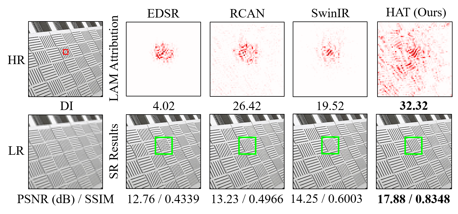
Figure 2: LAM [23] results for different networks. The results indicate that SwinIR utilizes less information compared to RCAN, while HAT uses the most pixels for reconstruction.

Besides, we can observe obvious blocking artifacts in the intermediate features of SwinIR, as shown in Fig. 3. These artifacts are caused by the window partition mechanism, which suggests that the shifted window mechanism is inefficient to build the cross-window connection. This may also be the reason why SwinIR do not utilize more pixels for the reconstruction in Fig. 2. Some works for high-level vision tasks [47, 46, 49, 52] also point out that enhancing the connection among windows can improve the window-based self-attention methods. Thus, we strengthen cross-window information interactions when designing our approach, and the blocking artifacts in the intermediate features obtained by HAT are significantly alleviated.

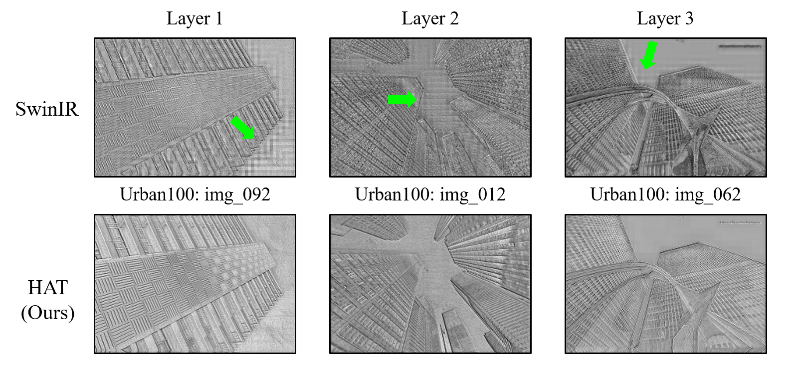
Figure 3: Intermediate features visualization of SwinIR [22] and HAT.“Layer N” represents the intermediate features after the $N_{th}$ layer (i.e., RSTB in SwinIR and RHAG in HAT.)

4 Methodology

4.1 Network Structure of HAT

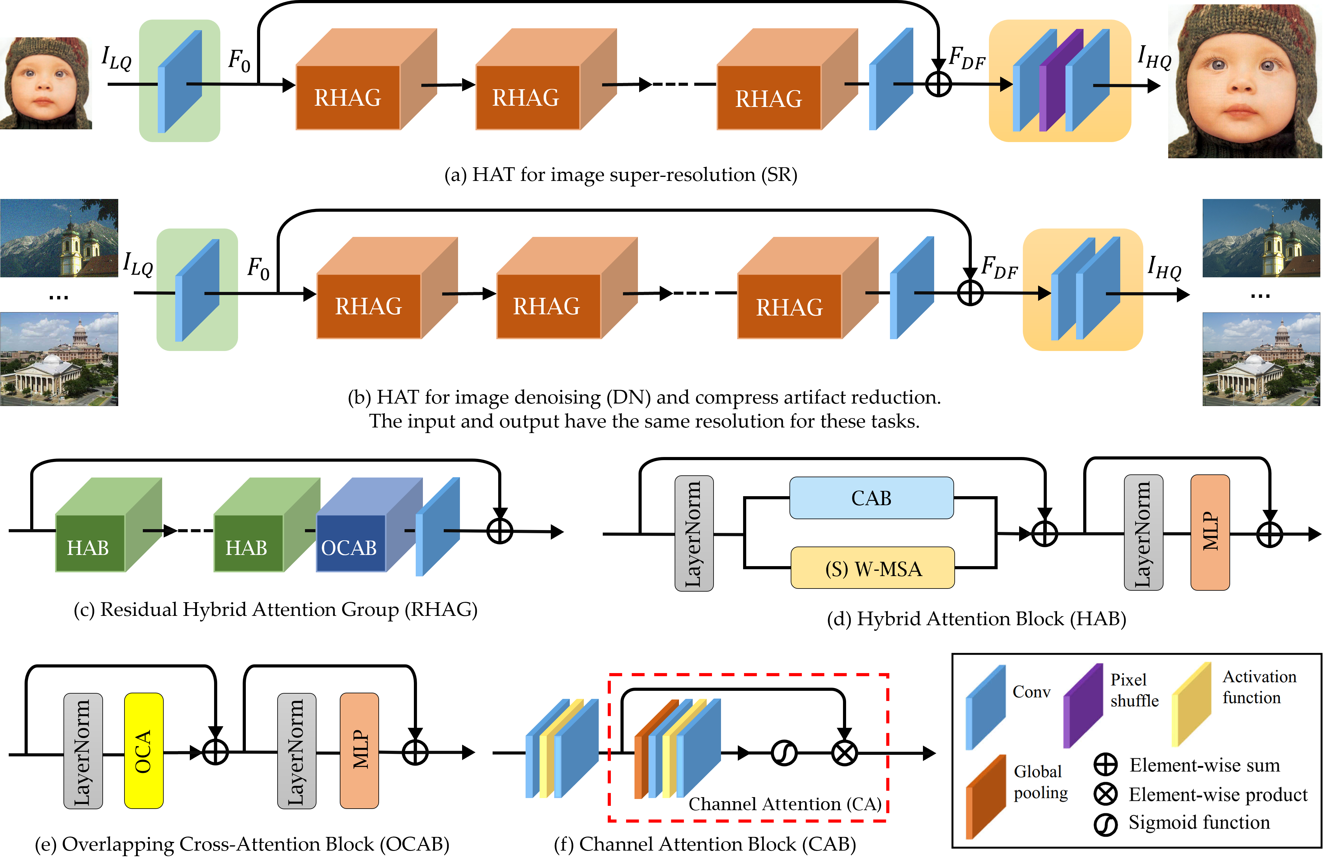
Figure 4: The overall architecture of HAT and the structure of RHAG and HAB.

The overall network structure of HAT follows the classic Residual in Residual (RIR) architecture similar to [10, 22]. As shown in Fig. 4, our HAT consists of three parts, including shallow feature extraction, deep feature extraction and image reconstruction. Concretely, for a given low-quality (LQ) input image $I_{LQ}\in\mathbb{R}^{H\times W\times C_{in}}$, we first use one $3\times 3$ convolution layer $H_{Conv}(\cdot)$ to extract the shallow feature $F_{0}\in\mathbb{R}^{H\times W\times C}$ as

$$F_{0}=H_{SF}(I_{LQ}),$$ (9)

where $C_{in}$ and $C$ denote the channel number of the input and the intermediate feature, respectively. The shallow feature extraction can simply map the input from low-dimensional space to high-dimensional space, while achieving the high-dimensional embedding for each pixel token. Moreover, the early convolution layer can help learn better visual representation [51] and lead to stable optimization [62]. We then perform deep feature extraction $H_{DF}(\cdot)$ to further obtain the deep feature $F_{DF}\in\mathbb{R}^{H\times W\times C}$ as

$$F_{DF}=H_{DF}(F_{0}),$$ (10)

where $H_{DF}(\cdot)$ consists of $N_{1}$ residual hybrid attention groups (RHAG) and one $3\times 3$ convolution layer $H_{Conv}(\cdot)$. These RHAGs progressively process the intermediate features as

$$F_{i}=H_{RHAG_{i}}(F_{i-1}),i=1,2,...,N,$$

$$F_{DF}=H_{Conv}(F_{N}),$$ (11)

where $H_{RHAG_{i}}(\cdot)$ represents the $i$-th RHAG. Following [22], we also introduce a convolution layer at the tail of this part to better aggregate information of deep features. After that, we add a global residual connection to fuse shallow features and deep features, and then reconstruct the high-quality (HQ) result via a reconstruction module as

$$I_{HQ}=H_{Rec}(F_{0}+F_{DF}),$$ (12)

where $H_{Rec}(\cdot)$ denotes the reconstruction module. We adopt the pixel-shuffle method [26] to up-sample the fused feature for the SR task shown in Fig. 4(a), and use two convolutions for the tasks where have the input and output have the same resolution shown in Fig. 4(b). The key component RHAG consists of $N_{2}$ hybrid attention blocks (HAB), one overlapping cross-attention block (OCAB), one $3\times 3$ convolution layer, with a residual connection, as presented in Fig. 4(c).

4.2 Hybrid Attention Block

We present details about our proposed hybrid attention block (HAB) shown in Fig. 4(d). We adopt similar structure of standard Swin Transformer block and preserve the window-based self-attention mechanism to build the HAB, but enhance the representative ability of the self-attention and introduce the channel attention block into it.

As discussed in Sec. 3.2, we aim to activate more input pixels for Transformer to obtain stronger reconstruction capability. Unlike convolution that expands the receptive field by stacking layers, self-attention has a global receptive field within its scope of action. Therefore, an intuitive way to expand the scope of utilized information for window-based self-attention is to enlarge the window size. Previous work [22] limits the window size for the calculation of self-attention to a small range (i.e., 7 or 8), relying on the shifted window mechanism to gradually expand the receptive field. This approach saves computational cost, but sacrifices the ability of self-attention. As discussed in Sec. 5.1, we find that window size is a crucial factor affecting the ability of window-based Self-attention to exploit information, and appropriately increasing the window size can significantly improve the performance of Transformer. Therefore, we adopt a large window size (i.e., 16) in our HAB.

In addition, more pixels are activated when channel attention is adopted, as global information is involved to calculate the channel attention weights. We think that the global information may help for cases where many similar textures exist, such as the examples given in Fig. 2. Besides, several works [20, 71] have demonstrated that the channel-wise dynamic mapping is beneficial for low-level vision tasks. Therefore, we want to introduce the channel attention mechanism to our network. Since many works have shown that convolution can help Transformer get better visual representation or achieve easier optimization [45, 62, 50, 51, 76], we incorporate a channel attention-based convolution block, i.e., the channel attention block (CAB) in Fig. 4(f), into the standard Transformer block to build our HAB.

To avoid the possible conflict of CAB and MSA on optimization and visual representation, we combine them in parallel and set a small constant $\alpha$ to control the weight of the CAB output. Overall, for a given input feature $X$, the whole process of HAB is computed as

$$X_{N}={\rm LN}(X),$$

$$X_{M}={\rm\text{(S)W-MSA}}(X_{N})+\alpha{\rm CAB}(X_{N})+X,$$ (13)

$$Y={\rm MLP}({\rm LN}(X_{M}))+X_{M},$$

where $X_{N}$ and $X_{M}$ denote the intermediate features. $Y$ represents the output of HAB. LN represents the layer normalization operation and MLP denotes a multi-layer perceptron. (S)W-MSA means the standard and shifted window multihead self-attention modules. Especially, we treat each pixel as a token for embedding (i.e., set patch size as 1 for patch embedding following [22]). For calculation of the self-attention module, given an input feature of size $H\times W\times C$, it is first partitioned into $\frac{HW}{M^{2}}$ local windows of size $M\times M$, then self-attention is calculated inside each window. For a local window feature $X_{W}\in\mathbb{R}^{M^{2}\times C}$, the query, key and value matrices are computed by linear mappings as $Q$, $K$ and $V$. Then the window-based self-attention is formulated as

$${\rm Attention}(Q,K,V)={\rm SoftMax}(QK^{T}/\sqrt{d}+B)V,$$ (14)

where $d$ represents the dimension of query/key. $B$ denotes the relative position encoding and is calculated as [14]. Besides, to build the connections between neighboring non-overlapping windows, we also utilize the shifted window partitioning approach [16] and set the shift size to half of the window size.

A CAB consists of two standard convolution layers with a GELU activation [77] and a channel attention (CA) module, as shown in Fig. 4(f). Since the Transformer-based structure often requires a large number of channels for token embedding, directly using convolutions with constant width incurs a large computation cost. Thus, we compress the channel numbers of the two convolution layers by a constant $\beta$. For an input feature with $C$ channels, the channel number of the output feature after the first convolution layer is squeezed to $\frac{C}{\beta}$, then the feature is expanded to $C$ channels through the second layer. Next, a standard CA module  [10] is exploited to adaptively rescale channel-wise features.

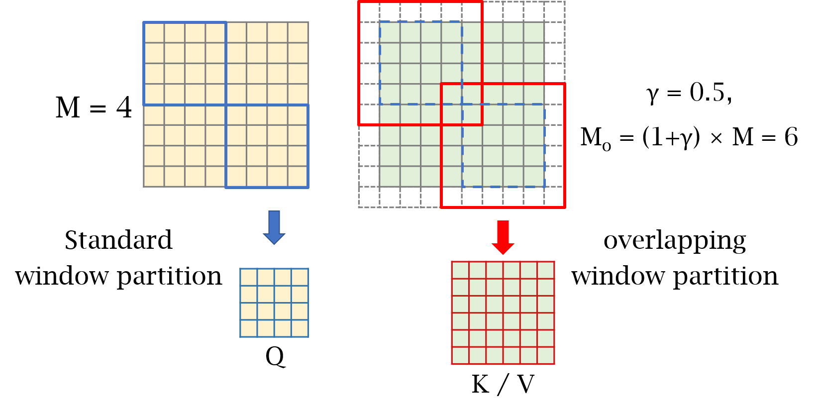
Figure 5: The overlapping window partition for OCA.

4.3 Overlapping Cross-Attention Block (OCAB)

We introduce OCAB to directly establish cross-window connections and enhance the representative ability for the window self-attention. Our OCAB consists of an overlapping cross-attention (OCA) layer and an MLP layer similar to the standard Swin Transformer block [16]. But for OCA, as depicted in Fig. 5, we use different window sizes to partition the projected features. Specifically, for the $X_{Q},X_{K},X_{V}\in\mathbb{R}^{H\times W\times C}$ of the input feature $X$, $X_{Q}$ is partitioned into $\frac{HW}{M^{2}}$ non-overlapping windows of size ${M}\times{M}$, while $X_{K},X_{V}$ are unfolded to $\frac{HW}{M^{2}}$ overlapping windows of size ${M_{o}}\times{M_{o}}$. It is calculated as

$$M_{o}=(1+\gamma)\times M,$$ (15)

where $\gamma$ is a constant to control the overlapping size. To better understand this operation, the standard window partition can be considered as a sliding partition with the kernel size and the stride both equal to the window size $M$. In contrast, the overlapping window partition can be viewed as a sliding partition with the kernel size equal to $M_{o}$, while the stride is equal to $M$. Zero-padding with size $\frac{\gamma M}{2}$ is used to ensure the size consistency of overlapping windows. The attention matrix is calculated as Eq. (14), and the relative position bias $B\in\mathbb{R}^{M\times M_{o}}$ is also adopted. Unlike WSA whose query, key and value are calculated from the same window feature, OCA computes key/value from a larger field where more useful information can be utilized for the query. Note that although Multi-resolution Overlapped Attention (MOA) module in [52] performs similar overlapping window partition, our OCA is fundamentally different from MOA. MOA calculates global attention using window features as tokens, while OCA computes cross-attention inside each window feature using pixel tokens.

4.4 The Same-task Pre-training

Pre-training is proven effective on many high-level vision tasks [15, 78, 79]. Recent works [18, 21] also demonstrate that pre-training is beneficial to low-level vision tasks. IPT [18] emphasizes the use of various low-level tasks, such as denoising, deraining, super-resolution and etc., while EDT [21] utilizes different degradation levels of a specific task to do pre-training. These works focus on investigating the effect of multi-task pre-training for a target task. In contrast, we directly perform pre-training on a larger-scale dataset (i.e., ImageNet [80]) based on the same task, showing that the effectiveness of pre-training depends more on the scale and diversity of data. For example, when we want to train a model for $\times 4$ SR, we first train a $\times 4$ SR model on ImageNet, then fine-tune it on the specific dataset, such as DF2K. The proposed strategy, namely same-task pre-training, is simpler while bringing more performance improvements. It is worth mentioning that sufficient training iterations for pre-training and an appropriate small learning rate for fine-tuning are very important for the effectiveness of the pre-training strategy. We think that it is because Transformer requires more data and iterations to learn general knowledge for the task, but needs a small learning rate for fine-tuning to avoid overfitting to the specific dataset.

4.5 Discussions

In this part, we analyze the distinctions of our HAT and several relevant works, including SwinIR [22], IPT [18], EDT [21] and HaloNet [54]

Difference to SwinIR. SwinIR [22] is the first work to successfully use Swin Transformer [16] for low-level vision tasks. It builds an image restoration network by using the original Swin Transformer block. The design of our HAT is inspired by SwinIR and retains the core design of window-based self-attention in SwinIR. However, we address the problem of limited range of utilized information in SwinIR by enlarging the window size and introducing channel attention. At the same time, we introduce a newly designed OCA to further enhance the ability of SwinIR to implement cross-window information interaction. Our HAT is a more powerful backbone for low-level vision tasks.

Difference to IPT. IPT [18] is an image processing Transformer based on the similar design of ViT [15]. It uses the patch token and calculates the global self-attention of features. The computational complexity of IPT grows quadratically with the input size. In contrast, our HAT adopts the pixel token and computes self-attention in the windows of fixed size. Therefore, in HAT, the computational complexity of Self-attention grows linearly with the input size. IPT also uses a pre-training strategy. Its multi-task pre-training strategy aims to utilize the correlation between multiple tasks. However, our pre-training is only performed on a single task to maximize the capability of the model on the specific task.

Difference to EDT. EDT [21] builds an image restoration Transformer based on the shifted crossed local attention, which also calculates self-attention in the windows of fixed size. For a given feature map, it splits the feature into two parts and performs self-attention in an either horizontal or vertical rectangle window. In contrast, our HAT adopts the vanilla window-based self-attention and shifted window mechanism similar to Swin Transformer [16]. EDT also studies the pre-training strategy and emphasizes the advantages of multi-related-task pre-training (i.e., performing pre-training on a specific task with multiple degradation levels). However, our HAT shows that training on the same task but using a large-scale dataset is the key factor in the effectiveness of pre-training.

Difference to HaloNet. HaloNet [54] incorporates a similar window partition mechanism to our OCA, enabling the calculation of self-attention within overlapping window features. HaloNet employs this overlapping self-attention as the fundamental module to build the network, inevitably leading to a large computational cost. This design could impose a substantial computational burden and is not friendly to image restoration tasks. On the contrary, our HAT leverages only a limited number of OCA modules to augment the interaction between adjacent windows. This approach can effectively enhance the image restoration Transformer without incurring excessive computational costs.

TABLE I: Quantitative results on PSNR(dB) for different window sizes.

Size	Set5	Set14	BSD100	Urban100	Manga109
(8,8)	32.88	29.09	27.92	27.45	32.03
(16,16)	32.97	29.12	27.95	27.81	32.15

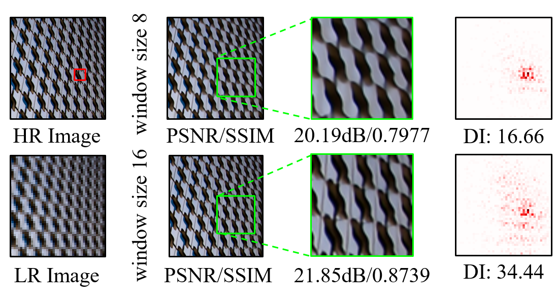
Figure 6: Qualitative comparison of different window sizes.

4.6 Implementation Details

For the structure of HAT, both the RHAG number and HAB number are set to 6. The channel number of the whole network is set to 180. The attention head number and window size are set to 6 and 16 for both (S)W-MSA and OCA. For the specific hyper-parameters of the proposed modules, we set the weighting factor of CAB output ($\alpha$), the squeeze factor between two convolution layers in CAB ($\beta$), and the overlapping ratio of OCA ($\gamma$) as 0.01, 3 and 0.5, respectively. For the large variant HAT-L, we double the depth of HAT by increasing the RHAG number from 6 to 12. We also provide a small version HAT-S with fewer parameters and similar computation to SwinIR. For HAT-S, we set the channel number to 144 and set $\beta$ to 24 in CAB. When implementing the pre-training strategy, we adopt ImageNet [80] as the pre-training dataset following [18, 21]. We conduct the main experiments and ablation study on image SR. Therefore, we use the DF2K dataset (DIV2K [81]+Flicker2K [82]) as the training dataset, following [22, 83]. PSNR/SSIM calculated on the Y channel is reported for the quantitative metrics.

TABLE II: Ablation study on the proposed OCAB and CAB.

	Baseline
OCAB	X	✓	X	✓
CAB	X	X	✓	✓
Set5	32.99dB	33.02dB	33.00dB	33.04dB
Set14	29.13dB	29.19dB	29.16dB	29.23dB
Urban100	27.81dB	27.91dB	27.91dB	27.97dB

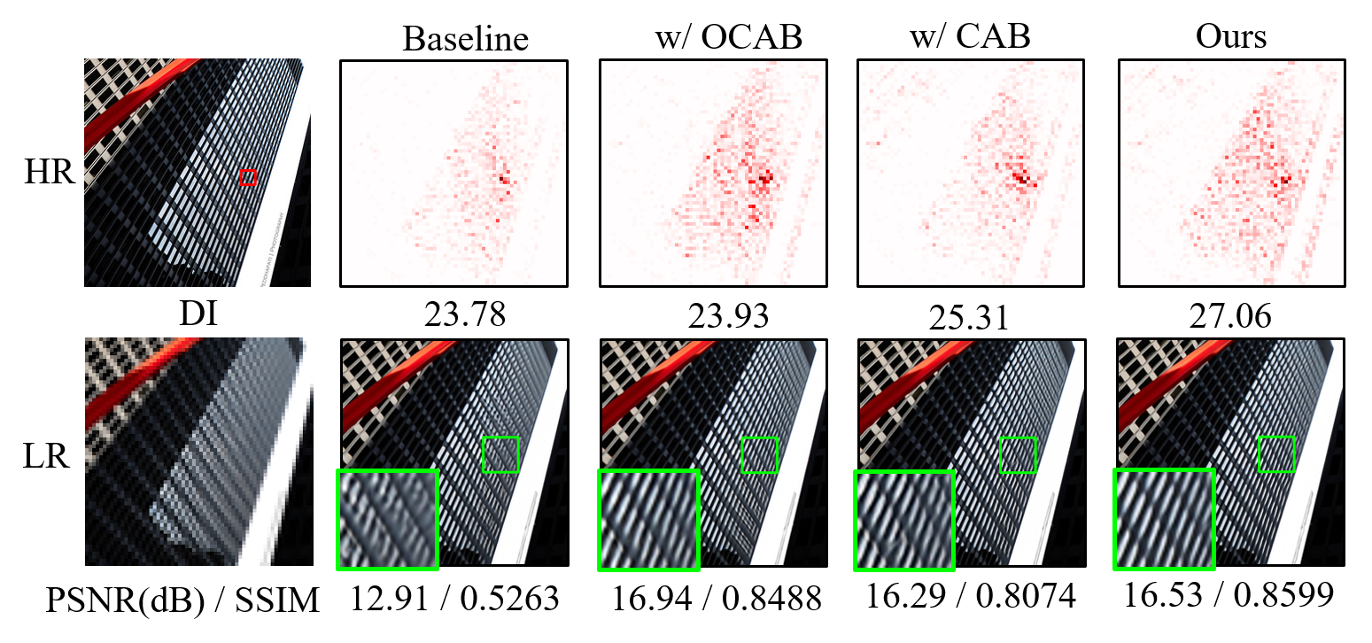
Figure 7: Ablation study on the proposed OCAB and CAB.

5 Network Investigation

5.1 Effects of different window sizes

As discussed in Sec. 3.2, activating more input pixels for the restoration tends to achieve better performance. Enlarging window size for the window-based self-attention is an intuitive way to realize the goal. In this section, we explore how the window size of self-attention influences the performance of Transformer on image SR. To eliminate the influence of our newly-introduced blocks, we conduct the following experiments directly on the preliminary version of SwinIR. As shown in Tab. I, the model with a large window size of 16$\times$16 obtains better performance, especially on Urban100. We also provide the qualitative comparison in Fig. 6. The result produced by the model with a larger window size has much clearer textures. As for the LAM results, the model with window size of 16 utilizes much more input pixels than the model with window size of 8. There experiments demonstrate that enlarging the window size can effectively improve the performance of SR Transformer.

5.2 Ablation Study

Effectiveness of OCAB and CAB. We conduct experiments to demonstrate the effectiveness of the proposed CAB and OCAB. The quantitative performance reported on three benchmark datasets for $\times 4$ SR is shown in Tab. II. On Urban100, compared with the baseline results, both OCAB and CAB bring the performance gain of 0.1dB. Benefiting from the two modules, the model obtains a further performance gain of 0.16dB. On Set5 and Set14, the proposed OCAB and CAB can also bring considerable performance improvement. We think that the performance improvement comes from two aspects. On the one hand, improving the window interaction by OCAB and utilizing the global statistics by CAB both help the model better deal with the long-term patters (e.g., self-similarity of repeated textures). On the other hand, the two modules enrich and enhance the model ability by introducing cross-attention and convolution blocks. We also provide qualitative comparison to further illustrate the influence of OCAB and CAB, as presented in Fig. 7. We can observe that the model with OCAB has a larger scope of the utilized pixels and generate better-reconstructed results. When CAB is adopted, the used pixels even expand to almost the full image. Moreover, the result of our method with OCAB and CAB obtains the highest DI[23], which means our method utilizes the most input pixels.

TABLE III: Effects of the channel attention (CA) module in CAB.

Structure	w/o CA	w/ CA
PSNR / SSIM	27.92dB / 0.8362	27.97dB / 0.8367

TABLE IV: Effects of the weighting factor $\alpha$ in CAB.

$\alpha$	0	1	0.1	0.01
PSNR	27.81dB	27.86dB	27.90dB	27.97dB

TABLE V: Ablation study on the overlapping ratio of OCAB.

$\gamma$	0	0.25	0.5	0.75
PSNR	27.85dB	27.81dB	27.91dB	27.86dB

Effects of different designs of CAB. We conduct experiments to explore the effects of different designs of CAB. First, we investigate the influence of channel attention. As shown in Tab. III, the model using CA achieves a performance gain of 0.05dB compared to the model without CA. It demonstrates the effectiveness of the channel attention in our network. We also conduct experiments to explore the effects of the weighting factor $\alpha$ of CAB. As presented in Sec. 4.2, $\alpha$ is used to control the weight of CAB features for feature fusion. A larger $\alpha$ means a larger weight of features extracted by CAB and $\alpha=0$ represents CAB is not used. As shown in Tab. IV, the model with $\alpha$ of 0.01 obtains the best performance. It indicates that CAB and self-attention may have potential issue in optimization, while a small weighting factor for the CAB branch can suppress this issue for the better combination.

Effects of the overlapping ratio. In OCAB, we set a constant $\gamma$ to control the overlapping size for the overlapping cross-attention, as illustrated in Sec 4.3. To explore the effects of different overlapping ratios, we set a group of $\gamma$ from 0 to 0.75 to examine the performance change, as shown in Tab. V. Note that $\gamma=0$ means a standard Transformer block. It can be found that the model with $\gamma=0.5$ performs best. In contrast, when $\gamma$ is set to 0.25 or 0.75, the model has no obvious performance gain or even has a performance drop. It illustrates that inappropriate overlapping size cannot benefit the interaction of neighboring windows.

TABLE VI: Model complexity for different window sizes.

window size	$\#$Params.	$\#$Multi-Adds.	PSNR
(8, 8)	11.9M	53.6G	27.45dB
(16, 16)	12.1M	63.8G	27.81dB

TABLE VII: Model complexity for OCAB and CAB.

Method	$\#$Params.	$\#$Multi-Adds.	PSNR
Baseline	12.1M	63.8G	27.81dB
w/ OCAB	13.7M	74.7G	27.91dB
w/ CAB	19.2M	92.8G	27.91dB
Ours	20.8M	103.7G	27.97dB

TABLE VIII: Model complexity for different CAB sizes.

$\beta$ in CAB	$\#$Params.	$\#$Multi-Adds.	PSNR
1	33.2M	150.1G	27.97dB
2	22.7M	107.1G	27.92dB
3 (default)	19.2M	92.8G	27.91dB
6	15.7M	78.5G	27.88dB
w/o CAB	12.1M	63.8G	27.81dB

TABLE IX: Model complexity comparison of SwinIR and HAT.

Method	$\#$Params.	$\#$Multi-Adds.	PSNR
SwinIR	11.9M	53.6G	27.45dB
HAT-S (ours)	9.6M	54.9G	27.80dB
SwinIR-L1	24.0M	104.4G	27.53dB
SwinIR-L2	23.1M	102.4G	27.58dB
HAT (ours)	20.8M	103.7G	27.97dB

5.3 Analysis of Model Complexity

We first conduct experiments to analyze the computational complexity of our method from three aspects: window size for the calculation of self-attention, ablation of OCAB and CAB, and the different designs of CAB. We evaluate the performance based on the results of $\times$4 SR on Urban100 and the number of Multiply-Add operations is counted at the input size of 64 $\times$ 64. Note that pre-training is Not used for all models in this section, and all methods are fairly compared under the same training settings.

First, we use the standard Swin Transformer block [22] as the backbone to explore the influence on different window sizes. As shown in Tab. VI, enlarging window size can bring a large performance gain (+0.36dB) with a little increase in parameters and $\sim$$\%19$ increase in Multi-Adds.

Then, we investigate the computational complexity of OCAB and CAB. As illustrated in Tab. VII, our OCAB obtains a performance gain with a limited increase of parameters and Multi-Adds. It demonstrates that the effectiveness and efficiency of the proposed OCAB. Adding CAB to the baseline model will increase the computational complexity, but it can achieves considerable performance improvement.

Since CAB seems to be computationally expensive, we further explore the influence on CAB sizes by modulating the squeeze factor $\beta$ (mentioned in Sec 4.2). As shown in Tab. VIII, adding a small CAB whose $\beta$ equals 6 can bring considerable performance improvement. When we continuously reduce $\beta$, the performance increases but with larger model sizes. To balance the performance and computations, we set $\beta$ to 3 as the default setting.

Furthermore, we compare HAT and SwinIR with the similar numbers of parameters and Multi-Adds in two settings, as presented in Tab. IX. First, we compare HAT-S with the original version of SwinIR. With less parameters and comparable computations, HAT-S significantly outperforms SwinIR. Second, we enlarge SwinIR by increasing the width and depth to achieve similar computations to HAT, denoted as SwinIR-L1 and SwinIR-L2. HAT achieves the best performance at the lowest computational cost. This demonstrates that HAT outperforms SwinIR not only in performance but also in computational efficiency.

Overall, we find that enlarging the window size for the calculation of self-attention is a very cost-effective way to improve the Transformer model. Moreover, the proposed OCAB can bring an obvious performance gain with limited increase of computations. Although CAB is not as efficient as above two schemes, it can also bring stable and considerable performance improvement. Benefiting from the three designs, HAT can substantially outperforms the state-of-the-art method SwinIR with comparable computations.

TABLE X: Quantitative results on PSNR(dB) of HAT using two kinds of pre-training strategies on $\times$4 SR under the same training setting.

Strategy	Stage	Set5	Set14	Urban100
Multi-related-task	pre-training	32.94	29.17	28.05
pre-training	fine-tuning	33.06	29.33	28.21
Same-task	pre-training	33.02	29.20	28.11
pre-training(ours)	fine-tuning	33.07	29.34	28.28

5.4 Study on the pre-training strategy

From Tab. XI, we can see that HAT can benefit greatly from the pre-training strategy, by comparing the performance of HAT and HAT^†. To show the superiority of the proposed same-task pre-training, we also apply the multi-related-task pre-training [21] to HAT for comparison using full ImageNet, under the same training settings as  [21]. As depicted as Tab. X, the same-task pre-training performs better, not only in the pre-training stage but also in the fine-tuning process. From this perspective, multi-task pre-training probably impairs the restoration performance of the network on a specific degradation, while the same-task pre-training can maximize the performance gain brought by large-scale data. To further investigate the influences of our pre-training strategy for different networks, we apply our pre-training to four networks: SRResNet (1.5M), RRDBNet (16.7M), SwinIR (11.9M) and HAT (20.8M), as shown in Fig. 8. First, we can see that all four networks can benefit from pre-training, showing the effectiveness of the proposed same-task pre-training strategy. Second, for the same type of network (i.e., CNN or Transformer), the larger the network capacity, the more performance gain from pre-training. Third, although with less parameters, SwinIR obtains greater performance improvement from the pre-training compared to RRDBNet. It suggests that Transformer needs more data to exploit the potential of the model. HAT obtains the largest gain from pre-training, indicating the necessity of the pre-training strategy for such large models. Equipped with big models and large-scale data, we show that the performance upper bound of this task can be significantly extended.

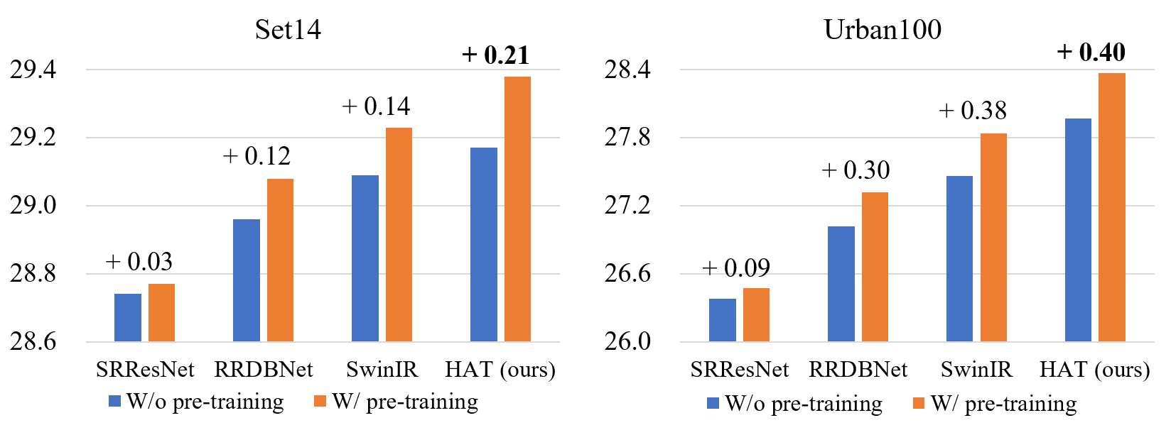
Figure 8: Quantitative comparison on PSNR(dB) of four different networks without and with the same-task pre-training on $\times$4 SR.

6 Experimental Results

6.1 Training Settings

For classic image super-resolution, we use DF2K (DIV2K + Flicker2K) with 3450 images as the training dataset when training from scratch. The low-resolution images are generated from the ground truth images by the “bicubic” down-sampling in MATLAB. We set the input patch size to $64\times 64$ and use random rotation and horizontally flipping for data augmentation. The mini-batch size is set to 32 and total training iterations are set to 500K. The learning rate is initialized as 2e-4 and reduced by half at [250K,400K,450K,475K]. For $\times$4 SR, we initialize the model with pre-trained $\times$2 SR weights and halve the iterations for each learning rate decay as well as total iterations. We adopt Adam optimizer with $\beta_{1}=0.9$ and $\beta_{2}=0.99$ to train the model. When using the same-task pre-training, we exploit the full ImageNet dataset with 1.28 million images to pre-train the model for 800K iterations. The initial learning rate is also set to 2e-4 but reduced by half at [300K,500K,650K,700K,750k]. Then, we adopt DF2K dataset to fine-tune the pre-trained model. For fine-tuning, we set the initial learning rate to 1e-5 and halve it at [125K,200K,230K,240K] for total 250K iterations.

TABLE XI: Quantitative comparison with state-of-the-art methods for classic image super-resolution on benchmark datasets. The best, second best and third best results are marked in red, blue and green. “$\dagger$” indicates that methods adopt pre-training strategy on ImageNet.

Method	Scale	Training Dataset	Set5 [84]		Set14 [85]		BSD100 [86]		Urban100 [87]		Manga109 [88]
			PSNR	SSIM	PSNR	SSIM	PSNR	SSIM	PSNR	SSIM	PSNR	SSIM
EDSR [28]	$\times$2	DIV2K	38.11	0.9602	33.92	0.9195	32.32	0.9013	32.93	0.9351	39.10	0.9773
RCAN [10]	$\times$2	DIV2K	38.27	0.9614	34.12	0.9216	32.41	0.9027	33.34	0.9384	39.44	0.9786
SAN [30]	$\times$2	DIV2K	38.31	0.9620	34.07	0.9213	32.42	0.9028	33.10	0.9370	39.32	0.9792
IGNN [36]	$\times$2	DIV2K	38.24	0.9613	34.07	0.9217	32.41	0.9025	33.23	0.9383	39.35	0.9786
HAN [31]	$\times$2	DIV2K	38.27	0.9614	34.16	0.9217	32.41	0.9027	33.35	0.9385	39.46	0.9785
NLSN [32]	$\times$2	DIV2K	38.34	0.9618	34.08	0.9231	32.43	0.9027	33.42	0.9394	39.59	0.9789
RCAN-it [83]	$\times$2	DF2K	38.37	0.9620	34.49	0.9250	32.48	0.9034	33.62	0.9410	39.88	0.9799
SwinIR [22]	$\times$2	DF2K	38.42	0.9623	34.46	0.9250	32.53	0.9041	33.81	0.9427	39.92	0.9797
EDT [21]	$\times$2	DF2K	38.45	0.9624	34.57	0.9258	32.52	0.9041	33.80	0.9425	39.93	0.9800
HAT-S (ours)	$\times$2	DF2K	38.58	0.9628	34.70	0.9261	32.59	0.9050	34.31	0.9459	40.14	0.9805
HAT (ours)	$\times$2	DF2K	38.63	0.9630	34.86	0.9274	32.62	0.9053	34.45	0.9466	40.26	0.9809
IPT† [18]	$\times$2	ImageNet	38.37	-	34.43	-	32.48	-	33.76	-	-	-
EDT† [21]	$\times$2	DF2K	38.63	0.9632	34.80	0.9273	32.62	0.9052	34.27	0.9456	40.37	0.9811
HAT† (ours)	$\times$2	DF2K	38.73	0.9637	35.13	0.9282	32.69	0.9060	34.81	0.9489	40.71	0.9819
HAT-L† (ours)	$\times$2	DF2K	38.91	0.9646	35.29	0.9293	32.74	0.9066	35.09	0.9505	41.01	0.9831
EDSR [28]	$\times$3	DIV2K	34.65	0.9280	30.52	0.8462	29.25	0.8093	28.80	0.8653	34.17	0.9476
RCAN [10]	$\times$3	DIV2K	34.74	0.9299	30.65	0.8482	29.32	0.8111	29.09	0.8702	34.44	0.9499
SAN [30]	$\times$3	DIV2K	34.75	0.9300	30.59	0.8476	29.33	0.8112	28.93	0.8671	34.30	0.9494
IGNN [36]	$\times$3	DIV2K	34.72	0.9298	30.66	0.8484	29.31	0.8105	29.03	0.8696	34.39	0.9496
HAN [31]	$\times$3	DIV2K	34.75	0.9299	30.67	0.8483	29.32	0.8110	29.10	0.8705	34.48	0.9500
NLSN [32]	$\times$3	DIV2K	34.85	0.9306	30.70	0.8485	29.34	0.8117	29.25	0.8726	34.57	0.9508
RCAN-it [83]	$\times$3	DF2K	34.86	0.9308	30.76	0.8505	29.39	0.8125	29.38	0.8755	34.92	0.9520
SwinIR [22]	$\times$3	DF2K	34.97	0.9318	30.93	0.8534	29.46	0.8145	29.75	0.8826	35.12	0.9537
EDT [21]	$\times$3	DF2K	34.97	0.9316	30.89	0.8527	29.44	0.8142	29.72	0.8814	35.13	0.9534
HAT-S (ours)	$\times$3	DF2K	35.01	0.9325	31.05	0.8550	29.50	0.8158	30.15	0.8879	35.40	0.9547
HAT (ours)	$\times$3	DF2K	35.07	0.9329	31.08	0.8555	29.54	0.8167	30.23	0.8896	35.53	0.9552
IPT† [18]	$\times$3	ImageNet	34.81	-	30.85	-	29.38	-	29.49	-	-	-
EDT† [21]	$\times$3	DF2K	35.13	0.9328	31.09	0.8553	29.53	0.8165	30.07	0.8863	35.47	0.9550
HAT† (ours)	$\times$3	DF2K	35.16	0.9335	31.33	0.8576	29.59	0.8177	30.70	0.8949	35.84	0.9567
HAT-L† (ours)	$\times$3	DF2K	35.28	0.9345	31.47	0.8584	29.63	0.8191	30.92	0.8981	36.02	0.9576
EDSR [28]	$\times$4	DIV2K	32.46	0.8968	28.80	0.7876	27.71	0.7420	26.64	0.8033	31.02	0.9148
RCAN [10]	$\times$4	DIV2K	32.63	0.9002	28.87	0.7889	27.77	0.7436	26.82	0.8087	31.22	0.9173
SAN [30]	$\times$4	DIV2K	32.64	0.9003	28.92	0.7888	27.78	0.7436	26.79	0.8068	31.18	0.9169
IGNN [36]	$\times$4	DIV2K	32.57	0.8998	28.85	0.7891	27.77	0.7434	26.84	0.8090	31.28	0.9182
HAN [31]	$\times$4	DIV2K	32.64	0.9002	28.90	0.7890	27.80	0.7442	26.85	0.8094	31.42	0.9177
NLSN [32]	$\times$4	DIV2K	32.59	0.9000	28.87	0.7891	27.78	0.7444	26.96	0.8109	31.27	0.9184
RRDB [12]	$\times$4	DF2K	32.73	0.9011	28.99	0.7917	27.85	0.7455	27.03	0.8153	31.66	0.9196
RCAN-it [83]	$\times$4	DF2K	32.69	0.9007	28.99	0.7922	27.87	0.7459	27.16	0.8168	31.78	0.9217
SwinIR [22]	$\times$4	DF2K	32.92	0.9044	29.09	0.7950	27.92	0.7489	27.45	0.8254	32.03	0.9260
EDT [21]	$\times$4	DF2K	32.82	0.9031	29.09	0.7939	27.91	0.7483	27.46	0.8246	32.05	0.9254
HAT-S (ours)	$\times$4	DF2K	32.92	0.9047	29.15	0.7958	27.97	0.7505	27.87	0.8346	32.35	0.9283
HAT (ours)	$\times$4	DF2K	33.04	0.9056	29.23	0.7973	28.00	0.7517	27.97	0.8368	32.48	0.9292
IPT† [18]	$\times$4	ImageNet	32.64	-	29.01	-	27.82	-	27.26	-	-	-
EDT† [21]	$\times$4	DF2K	33.06	0.9055	29.23	0.7971	27.99	0.7510	27.75	0.8317	32.39	0.9283
HAT† (ours)	$\times$4	DF2K	33.18	0.9073	29.38	0.8001	28.05	0.7534	28.37	0.8447	32.87	0.9319
HAT-L† (ours)	$\times$4	DF2K	33.30	0.9083	29.47	0.8015	28.09	0.7551	28.60	0.8498	33.09	0.9335

For real-world image super-resolution, we use the pre-trained MSE-based model and then adopt DIV2k, Flick2K and OST [89] datasets for training, following [12, 38]. The LR-HR pairs are generated by the high-order degradation model [38]. The total batch size is set to 32 and the input patch size is set to $64\times 64$. The network structure is the same as the basic version of HAT for classic image super-resolution. Follwing Real-ESRGAN [38], we first train the MSE-based model and introduce the generative adversarial training to fine-tune the GAN-based model. More training and degradation details can refer to [38].

For image denoising and JPEG compression artifacts reduction, we directly use the combination of 800 DIV2K images, 2650 Flickr2K, 400 BSD500 images [86] and 4744 WED images [90] to train the models, following [68, 13, 22]. The network is the same as the basic version for classic image super-resolution without up-sampling. Noisy images are generated by adding additive white Gaussian noises with noise level $\sigma$ and compressed images are obtained by the MATLAB JPEG encoder with JPEG level $q$. To speed up the training, we first train models with the batch size of 32 and the patch size of $64\times 64$ for 800 iterations. We then proceed to fine-tune models with the batch size of 8 and the patch size of $128\times 128$ for 500 iterations.

6.2 Classic Image Super-Resolution

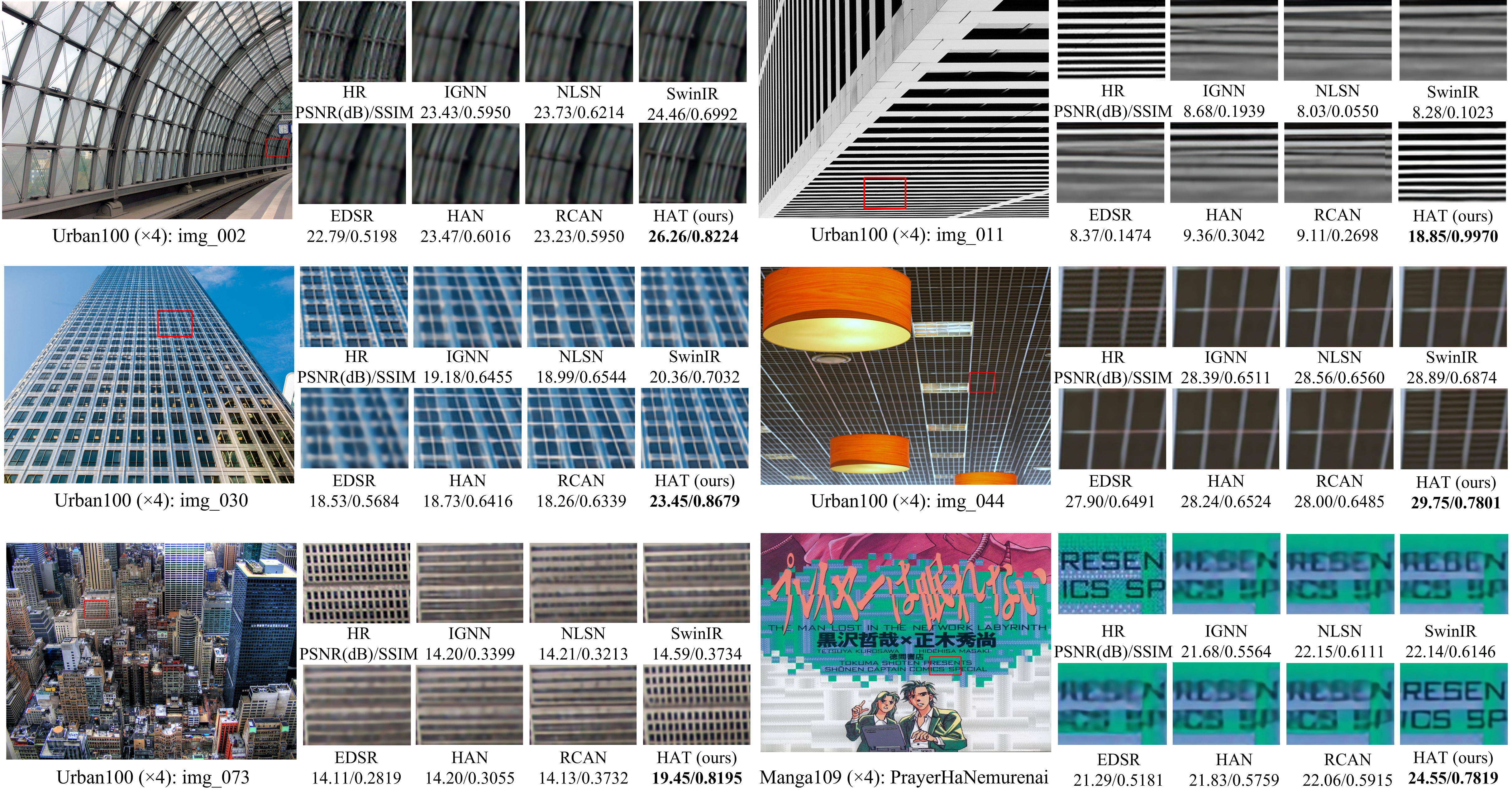
Figure 9: Visual comparison for $\times$4 SR. The patches for comparison are marked with red boxes in the original images. PSNR/SSIM is calculated based on the patches to better reflect the performance difference.

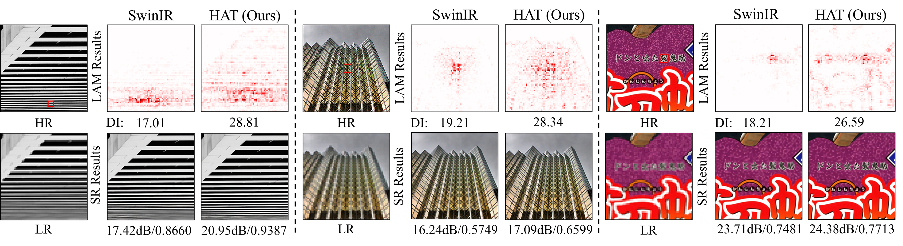
Figure 10: Comparison of LAM results between SwinIR and HAT.

Quantitative results. Tab. XI shows the quantitative comparison of our approach with the state-of-the-art methods: EDSR [28], RCAN [10], SAN [30], IGNN [36], HAN [31], NLSN [32], RCAN-it [83], as well as approaches using ImageNet pre-training, i.e., IPT [18] and EDT [21]. We can see that our method significantly outperforms the other methods on all five benchmark datasets. Concretely, with the same depth and width, HAT surpasses SwinIR by 0.48dB$\sim$0.64dB on Urban100 and 0.34dB$\sim$0.45dB on Manga109. When compared with the approaches using pre-training, HAT^† also has large performance gains of more than 0.5dB against EDT on Urban100 for all three scales. Besides, HAT equipped with pre-training outperforms SwinIR by a huge margin of up to 1dB on Urban100 for $\times$2 SR. Moreover, the large model HAT-L can even bring further improvement and greatly expands the performance upper bound of this task. HAT-S with fewer parameters and similar computation can also significantly outperforms the state-of-the-art method SwinIR. (Detailed computational complexity comparison can be found in Sec. 5.3.) Note that the performance gaps are much larger on Urban100, as it contains more structured and self-repeated patterns that can provide more useful pixels for reconstruction when the utilized range of information is enlarged. All these results show the effectiveness of our method.

Visual comparison. We provide the visual comparison as shown in Fig. 9. For the images “img 002”, “img 011”, “img 030”, “img 044” and “img 073” in the Urban100 dataset, HAT successfully recovers the clear lattice content. In contrast, the other approaches cannot restore correct textures or suffer from severe blurry effects. We can also observe similar behaviors on “PrayerHaNemurenai” in the Manga109 dataset. When recovering the characters in the image, HAT obtains much clearer textures than the other methods. The visual results also demonstrate the superiority of our approach on classic image super-resolution.

LAM comparison. We provide more visual results with LAM to compare the state-of-the method SwinIR and our HAT. As shown in Fig. 10, the utilized pixels for reconstruction of HAT expands to the almost full image, while that of SwinIR only gathers in a limited range. For the quantitative metric, HAT also obtains a much higher DI value than SwinIR. These results demonstrate that our method can activate more pixels to reconstruct the low-resolution input image. As a result, SR results generated by our method have higher PSNR/SSIM and better visual quality. We can observe that HAT restores much clearer textures and edges than SwinIR.

TABLE XII: Quantitative comparison with state-of-the-art methods for real-world image super-resolution on benchmark datasets. The best and second best results are marked in red and blue.

Method	RealSR-cano [91]		RealSR-Nikon [91]		AIM2019-val [92]		DIV2K-SysReal
	PSNR ($\uparrow$)	LPIPS ($\downarrow$)	PSNR ($\uparrow$)	LPIPS ($\downarrow$)	PSNR ($\uparrow$)	LPIPS ($\downarrow$)	PSNR ($\uparrow$)	LPIPS ($\downarrow$)
ESRGAN [12]	27.67	0.412	27.46	0.425	23.16	0.550	23.48	0.627
BSRGAN [93]	26.91	0.371	25.56	0.391	24.20	0.400	23.83	0.469
Real-ESRGAN [38]	26.14	0.378	25.49	0.388	23.89	0.396	23.58	0.446
SwinIR [22]	26.64	0.357	25.76	0.364	23.89	0.387	23.31	0.449
DASR [94]	27.40	0.393	26.35	0.401	23.76	0.421	23.78	0.473
HAT (ours)	26.68	0.342	25.85	0.358	24.19	0.370	23.98	0.423

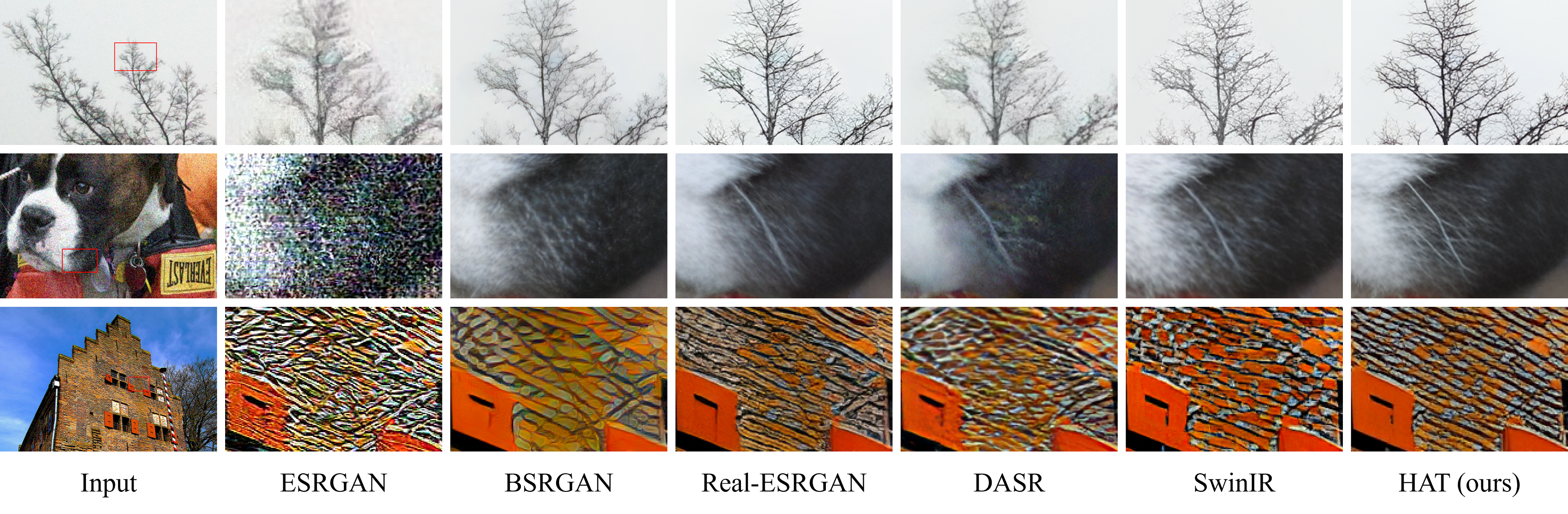
Figure 11: Real-world image super-resolution results on SR $\times 4$.

6.3 Real-world Image Super-Resolution

Quantitative results. Tab. XII shows the quantitative comparison on real-world image super-resolution of our method with the state-of-the-art approaches: ESRGAN [12], BSRGAN [93], Real-ESRGAN [38], DASR [94] and SwinIR [22]. Note that all these models are GAN-based models. Except for ESRGAN using Bicubic degradation, the others models are all trained based on real-world degradation models.

We use the officially released models for the compared methods and evaluate all the approaches on four datasets. Real-SR-cano [91] and Real-Nikon [91] consist of real-world data pairs captured by specific cameras. AIM2019-val, provided by the AIM2019 real-world image SR challenge [92], is a synthetic dataset that employs realistic and unknown degradations. Additionally, we construct a synthetic dataset based on 100 DIV2K valid [81] images using the high-order degradation model [38], following DASR [94]. For measurement, we adopt PSNR and LPIPS [95] as metrics, with PSNR reflecting the fidelity of the reconstruction, and LPIPS reflects the perceptual quality of results.

Since all of the methods are GAN-based, the PSNR performance of different models on various datasets is not consistent. Nevertheless, similar PSNR values indicate that the performance of the various methods in terms of fidelity is comparable. For LPIPS, HAT achieves the best performance on all four datasets, demonstrating that our method generates the results with the best perceptual quality.

Visual comparison. We present the visual results generated by different methods on real-world low-resolution images in Fig. 11. In the first and second rows of visual comparisons, our HAT generates clearer branches and whiskers than other methods. In the third row, the wall texture produced by HAT appears the most natural. Overall, our method is capable of producing visually pleasing results with clear and sharp edges. This demonstrates the great potential of our method for application in real-world scenarios.

6.4 Image Denoising

TABLE XIII: Quantitative comparison (average PSNR) with state-of-the-art methods for grayscale image denoising on benchmark datasets. The best, second best and third results are marked in red, blue and green,respectively.

Dataset	$\sigma$	BM3D [96]	DnCNN [7]	IRCNN [9]	FFDNet [67]	NLRN [39]	RNAN [11]	MWCNN [97]	DRUNet [13]	SwinIR [22]	Restormer [20]	HAT (ours)
Set12 [7]	15	32.37	32.86	32.76	32.75	33.16	-	33.15	33.25	33.36	33.42	33.43
	25	29.97	30.44	30.37	30.43	30.80	-	30.79	30.94	31.01	31.08	31.07
	50	26.72	27.18	27.12	27.32	27.64	27.70	27.74	27.90	27.91	28.00	27.97
BSD68 [86]	15	31.08	31.73	31.63	31.63	31.88	-	31.86	31.91	31.97	31.96	31.97
	25	28.57	29.23	29.15	29.19	29.41	-	29.41	29.48	29.50	29.52	29.51
	50	25.60	26.23	26.19	26.29	26.47	26.48	26.53	26.59	26.58	26.62	26.57
Urban100 [87]	15	32.35	32.64	32.46	32.40	33.45	-	33.17	33.44	33.70	33.79	33.90
	25	29.70	29.95	29.80	29.90	30.94	-	30.66	31.11	31.30	31.46	31.56
	50	25.95	26.26	26.22	26.50	27.49	27.65	27.42	27.96	27.98	28.29	28.28

TABLE XIV: Quantitative comparison (average PSNR) with state-of-the-art methods for color image denoising on benchmark datasets. The best, second best and third best results are marked in red, blue and green, respectively.

Dataset	$\sigma$	BM3D [96]	DnCNN [7]	IRCNN [9]	FFDNet [67]	RNAN [11]	RDN [29]	IPT [18]	DRUNet [13]	SwinIR [22]	Restormer [20]	HAT (ours)
CBSD68 [86]	15	33.52	33.90	33.86	33.87	-	-	-	34.30	34.42	34.40	34.42
	25	30.71	31.24	31.16	31.21	-	-	-	31.69	31.78	31.79	31.79
	50	27.38	27.95	27.86	27.96	28.27	28.31	28.39	28.51	28.56	28.60	28.58
Kodak24 [98]	15	34.28	34.60	34.69	34.63	-	-	-	35.31	35.34	35.47	35.50
	25	32.15	32.14	32.18	32.13	-	-	-	32.89	32.89	33.04	33.08
	50	28.46	28.95	28.93	28.98	29.58	29.66	29.64	29.86	29.79	30.01	30.02
McMaster [99]	15	34.06	33.45	34.58	34.66	-	-	-	35.40	35.61	35.61	35.64
	25	31.66	31.52	32.18	32.35	-	-	-	33.14	33.20	33.34	33.37
	50	28.51	28.62	28.91	29.18	29.72	-	29.98	30.08	30.22	30.30	30.26
Urban100 [87]	15	33.93	32.98	33.78	33.83	-	-	-	34.81	35.13	35.13	35.37
	25	31.36	30.81	31.20	31.40	-	-	-	32.60	32.90	32.96	33.14
	50	27.93	27.59	27.70	28.05	29.08	29.38	29.71	29.61	29.82	30.02	30.20

TABLE XV: Quantitative comparison (average PSNR/SSIM) with state-of-the-art methods for JPEG compression artifacts reduction on benchmark datasets. The best and second best results are marked in red and blue colors, respectively.

Dataset	$q$	ARCNN [6]	DnCNN [7]	RNAN [11]	RDN [29]	DRUNet [13]	SwinIR [22]	HAT (ours)
Classic5 [100]	10	29.03/0.7929	29.40/0.8026	29.96/0.8178	30.00/0.8188	30.16/0.8234	30.27/0.8249	30.27/0.8246
	20	31.15/0.8517	31.63/0.8610	32.11/0.8693	32.15/0.8699	32.39/0.8734	32.52/0.8748	32.54/0.8749
	30	32.51/0.8806	32.91/0.8861	33.38/0.8924	33.43/0.8930	33.59/0.8949	33.73/0.8961	33.72/0.8958
	40	33.32/0.8953	33.77/0.9003	34.27/0.9061	34.27/0.9061	34.41/0.9075	34.52/0.9082	34.58/0.9086
LIVE1 [101]	10	28.96/0.8076	29.19/0.8123	29.63/0.8239	29.67/0.8247	29.79/0.8278	29.86/0.8287	29.84/0.8283
	20	31.29/0.8733	31.59/0.8802	32.03/0.8877	32.07/0.8882	32.17/0.8899	32.25/0.8909	32.26/0.8907
	30	32.67/0.9043	32.98/0.9090	33.45/0.9149	33.51/0.9153	33.59/0.9166	33.69/0.9174	33.66/0.9170
	40	33.63/0.9198	33.96/0.9247	34.47/0.9299	34.51/0.9302	34.58/0.9312	34.67/0.9317	34.69/0.9317
Urban100 [87]	10	-	28.54/0.8487	29.76/0.8723	-	30.05/0.8872	30.55/0.8842	30.60/0.8845
	20	-	31.01/0.9022	32.33/0.9179	-	32.66/0.9216	33.12/0.9254	33.22/0.9260
	30	-	32.47/0.9248	33.83/0.9365	-	34.13/0.9392	34.58/0.9417	34.58/0.9419
	40	-	33.49/0.9376	34.95/0.9476	-	35.11/0.9491	35.50/0.9509	35.68/0.9517

6.4.1 Grayscale image denoising

Quantitative results. Tab. XIII shows the quantitative comparison on grayscale image denoising of our approach with the state-of-the-art method: BM3D [96], DnCNN [7], IRCNN [9], FFDNet [67], NLRN [39], MWCNN [97], DRUNet [13], SwinIR [22] and Restormer [20]. Compared to Restormer [20], our method achieves comparable performance and obtains performance gains of about 0.1dB on Urban100 with noise level $\sigma=15,25$. Compared to SwinIR [22], HAT achieves better performance on almost all three datasets with three noise levels. On Urban100, HAT achieves the most performance improvement, by up to 0.3dB for noise level $\sigma=50$.

Visual comparison. We provide the visual results of different methods in Fig. 12. For “09” in Set12, our HAT restores clear lines while other approaches suffers from severe blurs. For “test021” in BSD68 and “img 061” in Urban100, HAT reconstructs much sharper edges than other methods. For “img 076” in Urban100, the results produced by HAT have the clearest textures. Overall, our HAT obtains the best visual quality among all comparison methods.

6.4.2 Color image denoising

Quantitative results. Tab. XIV shows the quantitative comparison results on color image denoising of our approach with the state-of-the-art methods: BM3D [96], DnCNN [7], IRCNN [9], FFDNet [67], RNAN [11], RDN [68], IPT [18], DRUNet [13], SwinIR [22] and Restormer [20]. We can observe that HAT achieves the best performance on almost all four benchmark datasets. Specifically, HAT outperforms SwinIR by a margin of 0.24dB to 0.38dB and surpasses Restormer by a margin of 0.18dB to 0.24dB on Urban100.

Visual comparison. We present the visual results of different methods in Fig. 13. For images “img 039”, “img 042” and “img 074” on Urban100, HAT reconstructs complete and clear edges, whereas other methods cannot produce complete lines or suffer from severe blurring effects. For the image “img 085” on Urban100, our method successfully restores the correct shape and clear texture, while other methods all fail. All these results demonstrate the superiority of the proposed HAT on image denoising.

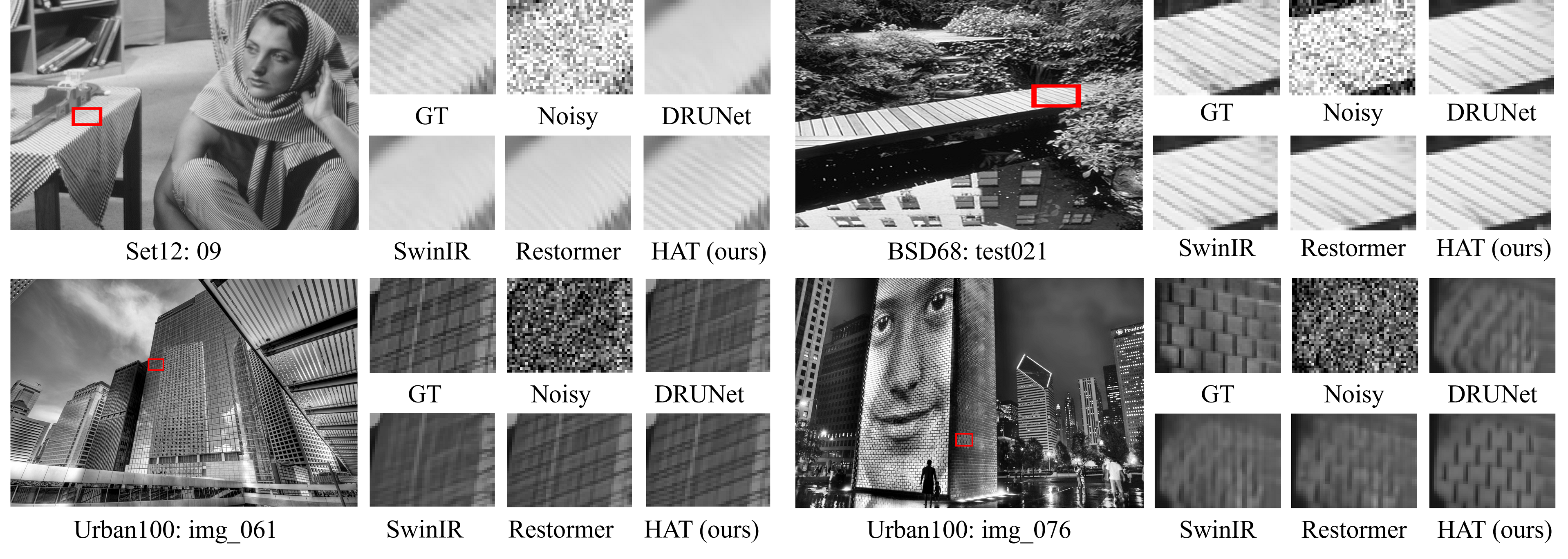
Figure 12: Grayscale image denoising results with noise level $\sigma=50$.

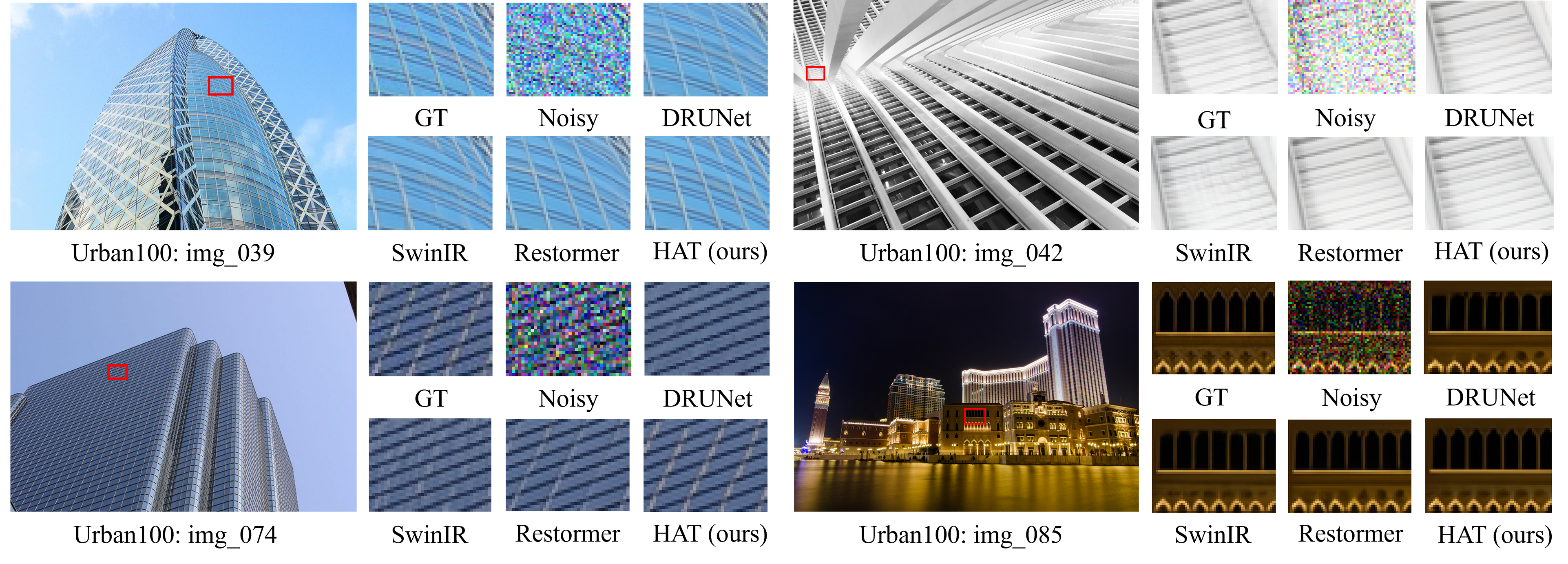
Figure 13: Color image denoising results with noise level $\sigma=50$.

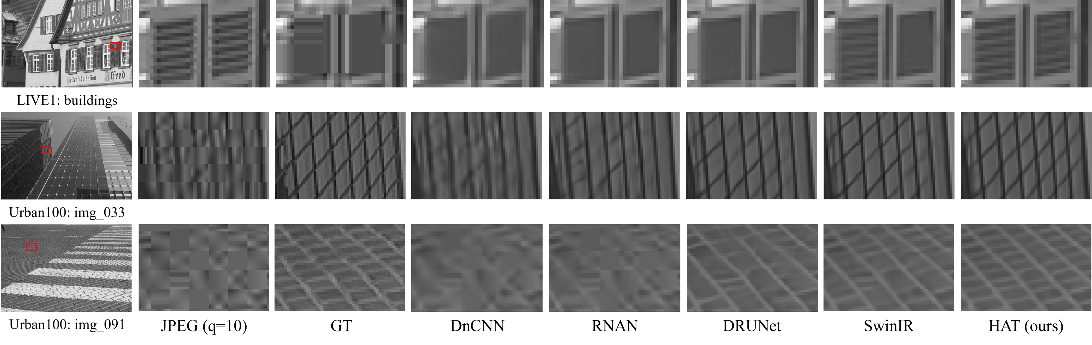
Figure 14: Image compression artifacts reduction results with JPEG quality $q=10$.

6.5 JPEG compression artifacts Reduction

Quantitative results. Tab. XV shows the quantitative comparison results on JPEG compression artifacts reduction of our approach with the state-of-the-art methods: ARCNN [6], DnCNN [7], RNAN [11], RDN [68], DRUNet [13], SwinIR [22]. On Classic5 and LIVE1, HAT only achieves comparable performance to SwinIR. We believe this is because the demand for the model fitting ability of this task has approached saturation, particularly for low-resolution images. We further provide the performance comparison on Urban100. Then we can see that HAT achieves considerable performance gains over SwinIR, up to 0.18dB for JPEG quality $q=40$. This can be attributed to the presence of a large number of regular textures and repeating patterns in the images of the Urban100 dataset. The proposed HAT is capable of activating more pixels for restoration. With a larger receptive field, HAT can reconstruct sharper edges and textures.

Visual comparison. We also provide the visual results of different approaches in Fig. 14. For the image “buildings” in LIVE1, HAT obtains much clearer textures than other methods, including SwinIR. For the self-repeated textures that appear in the images “img 033” and ‘img 091” of Urban100, our HAT successfully restores the correct results. All the quantitative and visual results demonstrate the superiority of our method on compression artifacts reduction.

7 Conclusion

In this work, we propose a new Hybrid Attention Transformer, HAT, for image restoration. Our model combines channel attention and self-attention to activate more pixels for high-resolution reconstruction. Besides, we propose an overlapping cross-attention module to enhance the interaction of cross-window information. Moreover, we introduce a same-task pre-training strategy for image super-resolution. Extensive benchmark and real-world evaluations demonstrate that our HAT outperforms the state-of-the-art methods for several image restoration tasks.

References

- [1] N. Fatima, “Ai in photography: Scrutinizing implementation of super-resolution techniques in photo-editors,” in 2020 35th International Conference on Image and Vision Computing New Zealand (IVCNZ). IEEE, 2020, pp. 1–6.
- [2] W. W. Zou and P. C. Yuen, “Very low resolution face recognition problem,” IEEE Transactions on image processing, vol. 21, no. 1, pp. 327–340, 2011.
- [3] W. Shi, J. Caballero, C. Ledig, X. Zhuang, W. Bai, K. Bhatia, A. M. S. M. de Marvao, T. Dawes, D. O’Regan, and D. Rueckert, “Cardiac image super-resolution with global correspondence using multi-atlas patchmatch,” in Medical Image Computing and Computer-Assisted Intervention–MICCAI 2013: 16th International Conference, Nagoya, Japan, September 22-26, 2013, Proceedings, Part III 16. Springer, 2013, pp. 9–16.
- [4] T. Karras, T. Aila, S. Laine, and J. Lehtinen, “Progressive growing of gans for improved quality, stability, and variation,” arXiv preprint arXiv:1710.10196, 2017.
- [5] C. Dong, C. C. Loy, K. He, and X. Tang, “Learning a deep convolutional network for image super-resolution,” in European conference on computer vision. Springer, 2014, pp. 184–199.
- [6] C. Dong, Y. Deng, C. C. Loy, and X. Tang, “Compression artifacts reduction by a deep convolutional network,” in Proceedings of the IEEE international conference on computer vision, 2015, pp. 576–584.
- [7] K. Zhang, W. Zuo, Y. Chen, D. Meng, and L. Zhang, “Beyond a gaussian denoiser: Residual learning of deep cnn for image denoising,” IEEE transactions on image processing, vol. 26, no. 7, pp. 3142–3155, 2017.
- [8] C. Dong, C. C. Loy, and X. Tang, “Accelerating the super-resolution convolutional neural network,” in European conference on computer vision. Springer, 2016, pp. 391–407.
- [9] K. Zhang, W. Zuo, S. Gu, and L. Zhang, “Learning deep cnn denoiser prior for image restoration,” in Proceedings of the IEEE conference on computer vision and pattern recognition, 2017, pp. 3929–3938.
- [10] Y. Zhang, K. Li, K. Li, L. Wang, B. Zhong, and Y. Fu, “Image super-resolution using very deep residual channel attention networks,” in Proceedings of the European conference on computer vision (ECCV), 2018, pp. 286–301.
- [11] Y. Zhang, K. Li, K. Li, B. Zhong, and Y. Fu, “Residual non-local attention networks for image restoration,” in International Conference on Learning Representations, 2018.
- [12] X. Wang, K. Yu, S. Wu, J. Gu, Y. Liu, C. Dong, Y. Qiao, and C. Change Loy, “Esrgan: Enhanced super-resolution generative adversarial networks,” in Proceedings of the European conference on computer vision (ECCV) workshops, 2018, pp. 0–0.
- [13] K. Zhang, Y. Li, W. Zuo, L. Zhang, L. Van Gool, and R. Timofte, “Plug-and-play image restoration with deep denoiser prior,” IEEE Transactions on Pattern Analysis and Machine Intelligence, vol. 44, no. 10, pp. 6360–6376, 2021.
- [14] A. Vaswani, N. Shazeer, N. Parmar, J. Uszkoreit, L. Jones, A. N. Gomez, Ł. Kaiser, and I. Polosukhin, “Attention is all you need,” Advances in neural information processing systems, vol. 30, 2017.
- [15] A. Dosovitskiy, L. Beyer, A. Kolesnikov, D. Weissenborn, X. Zhai, T. Unterthiner, M. Dehghani, M. Minderer, G. Heigold, S. Gelly et al., “An image is worth 16x16 words: Transformers for image recognition at scale,” in International Conference on Learning Representations, 2020.
- [16] Z. Liu, Y. Lin, Y. Cao, H. Hu, Y. Wei, Z. Zhang, S. Lin, and B. Guo, “Swin transformer: Hierarchical vision transformer using shifted windows,” in Proceedings of the IEEE/CVF International Conference on Computer Vision, 2021, pp. 10 012–10 022.
- [17] W. Wang, E. Xie, X. Li, D.-P. Fan, K. Song, D. Liang, T. Lu, P. Luo, and L. Shao, “Pyramid vision transformer: A versatile backbone for dense prediction without convolutions,” in Proceedings of the IEEE/CVF International Conference on Computer Vision, 2021, pp. 568–578.
- [18] H. Chen, Y. Wang, T. Guo, C. Xu, Y. Deng, Z. Liu, S. Ma, C. Xu, C. Xu, and W. Gao, “Pre-trained image processing transformer,” in Proceedings of the IEEE/CVF Conference on Computer Vision and Pattern Recognition, 2021, pp. 12 299–12 310.
- [19] Z. Wang, X. Cun, J. Bao, W. Zhou, J. Liu, and H. Li, “Uformer: A general u-shaped transformer for image restoration,” in Proceedings of the IEEE/CVF Conference on Computer Vision and Pattern Recognition, 2022, pp. 17 683–17 693.
- [20] S. W. Zamir, A. Arora, S. Khan, M. Hayat, F. S. Khan, and M.-H. Yang, “Restormer: Efficient transformer for high-resolution image restoration,” in Proceedings of the IEEE/CVF Conference on Computer Vision and Pattern Recognition, 2022, pp. 5728–5739.
- [21] W. Li, X. Lu, J. Lu, X. Zhang, and J. Jia, “On efficient transformer and image pre-training for low-level vision,” 2021.
- [22] J. Liang, J. Cao, G. Sun, K. Zhang, L. Van Gool, and R. Timofte, “Swinir: Image restoration using swin transformer,” in Proceedings of the IEEE/CVF International Conference on Computer Vision, 2021, pp. 1833–1844.
- [23] J. Gu and C. Dong, “Interpreting super-resolution networks with local attribution maps,” in Proceedings of the IEEE/CVF Conference on Computer Vision and Pattern Recognition, 2021, pp. 9199–9208.
- [24] X. Chen, X. Wang, J. Zhou, Y. Qiao, and C. Dong, “Activating more pixels in image super-resolution transformer,” in Proceedings of the IEEE/CVF Conference on Computer Vision and Pattern Recognition, 2023, pp. 22 367–22 377.
- [25] C. Dong, C. C. Loy, K. He, and X. Tang, “Image super-resolution using deep convolutional networks,” IEEE transactions on pattern analysis and machine intelligence, vol. 38, no. 2, pp. 295–307, 2015.
- [26] W. Shi, J. Caballero, F. Huszár, J. Totz, A. P. Aitken, R. Bishop, D. Rueckert, and Z. Wang, “Real-time single image and video super-resolution using an efficient sub-pixel convolutional neural network,” in Proceedings of the IEEE conference on computer vision and pattern recognition, 2016, pp. 1874–1883.
- [27] J. Kim, J. K. Lee, and K. M. Lee, “Accurate image super-resolution using very deep convolutional networks,” in Proceedings of the IEEE conference on computer vision and pattern recognition, 2016, pp. 1646–1654.
- [28] B. Lim, S. Son, H. Kim, S. Nah, and K. Mu Lee, “Enhanced deep residual networks for single image super-resolution,” in Proceedings of the IEEE conference on computer vision and pattern recognition workshops, 2017, pp. 136–144.
- [29] Y. Zhang, Y. Tian, Y. Kong, B. Zhong, and Y. Fu, “Residual dense network for image super-resolution,” in Proceedings of the IEEE conference on computer vision and pattern recognition, 2018, pp. 2472–2481.
- [30] T. Dai, J. Cai, Y. Zhang, S.-T. Xia, and L. Zhang, “Second-order attention network for single image super-resolution,” in Proceedings of the IEEE/CVF conference on computer vision and pattern recognition, 2019, pp. 11 065–11 074.
- [31] B. Niu, W. Wen, W. Ren, X. Zhang, L. Yang, S. Wang, K. Zhang, X. Cao, and H. Shen, “Single image super-resolution via a holistic attention network,” in European conference on computer vision. Springer, 2020, pp. 191–207.
- [32] Y. Mei, Y. Fan, and Y. Zhou, “Image super-resolution with non-local sparse attention,” in Proceedings of the IEEE/CVF Conference on Computer Vision and Pattern Recognition, 2021, pp. 3517–3526.
- [33] C. Ledig, L. Theis, F. Huszár, J. Caballero, A. Cunningham, A. Acosta, A. Aitken, A. Tejani, J. Totz, Z. Wang et al., “Photo-realistic single image super-resolution using a generative adversarial network,” in Proceedings of the IEEE conference on computer vision and pattern recognition, 2017, pp. 4681–4690.
- [34] J. Kim, J. K. Lee, and K. M. Lee, “Deeply-recursive convolutional network for image super-resolution,” in Proceedings of the IEEE conference on computer vision and pattern recognition, 2016, pp. 1637–1645.
- [35] Y. Tai, J. Yang, and X. Liu, “Image super-resolution via deep recursive residual network,” in Proceedings of the IEEE conference on computer vision and pattern recognition, 2017, pp. 3147–3155.
- [36] S. Zhou, J. Zhang, W. Zuo, and C. C. Loy, “Cross-scale internal graph neural network for image super-resolution,” Advances in neural information processing systems, vol. 33, pp. 3499–3509, 2020.
- [37] W. Zhang, Y. Liu, C. Dong, and Y. Qiao, “Ranksrgan: Generative adversarial networks with ranker for image super-resolution,” in Proceedings of the IEEE/CVF International Conference on Computer Vision, 2019, pp. 3096–3105.
- [38] X. Wang, L. Xie, C. Dong, and Y. Shan, “Real-esrgan: Training real-world blind super-resolution with pure synthetic data,” in Proceedings of the IEEE/CVF International Conference on Computer Vision, 2021, pp. 1905–1914.
- [39] D. Liu, B. Wen, Y. Fan, C. C. Loy, and T. S. Huang, “Non-local recurrent network for image restoration,” Advances in neural information processing systems, vol. 31, 2018.
- [40] Y. Liu, A. Liu, J. Gu, Z. Zhang, W. Wu, Y. Qiao, and C. Dong, “Discovering” semantics” in super-resolution networks,” 2021.
- [41] L. Xie, X. Wang, C. Dong, Z. Qi, and Y. Shan, “Finding discriminative filters for specific degradations in blind super-resolution,” Advances in Neural Information Processing Systems, vol. 34, 2021.
- [42] X. Kong, X. Liu, J. Gu, Y. Qiao, and C. Dong, “Reflash dropout in image super-resolution,” in Proceedings of the IEEE/CVF Conference on Computer Vision and Pattern Recognition, 2022, pp. 6002–6012.
- [43] Y. Liu, H. Zhao, J. Gu, Y. Qiao, and C. Dong, “Evaluating the generalization ability of super-resolution networks,” IEEE Transactions on Pattern Analysis and Machine Intelligence, 2023.
- [44] Y. Li, K. Zhang, J. Cao, R. Timofte, and L. Van Gool, “Localvit: Bringing locality to vision transformers,” 2021.
- [45] H. Wu, B. Xiao, N. Codella, M. Liu, X. Dai, L. Yuan, and L. Zhang, “Cvt: Introducing convolutions to vision transformers,” in Proceedings of the IEEE/CVF International Conference on Computer Vision, 2021, pp. 22–31.
- [46] Z. Huang, Y. Ben, G. Luo, P. Cheng, G. Yu, and B. Fu, “Shuffle transformer: Rethinking spatial shuffle for vision transformer,” 2021.
- [47] X. Dong, J. Bao, D. Chen, W. Zhang, N. Yu, L. Yuan, D. Chen, and B. Guo, “Cswin transformer: A general vision transformer backbone with cross-shaped windows,” in Proceedings of the IEEE/CVF Conference on Computer Vision and Pattern Recognition, 2022, pp. 12 124–12 134.
- [48] X. Chu, Z. Tian, Y. Wang, B. Zhang, H. Ren, X. Wei, H. Xia, and C. Shen, “Twins: Revisiting the design of spatial attention in vision transformers,” Advances in Neural Information Processing Systems, vol. 34, 2021.
- [49] S. Wu, T. Wu, H. Tan, and G. Guo, “Pale transformer: A general vision transformer backbone with pale-shaped attention,” in Proceedings of the AAAI Conference on Artificial Intelligence, vol. 36, no. 3, 2022, pp. 2731–2739.
- [50] K. Yuan, S. Guo, Z. Liu, A. Zhou, F. Yu, and W. Wu, “Incorporating convolution designs into visual transformers,” in Proceedings of the IEEE/CVF International Conference on Computer Vision, 2021, pp. 579–588.
- [51] K. Li, Y. Wang, J. Zhang, P. Gao, G. Song, Y. Liu, H. Li, and Y. Qiao, “Uniformer: Unifying convolution and self-attention for visual recognition,” IEEE Transactions on Pattern Analysis and Machine Intelligence, 2023.
- [52] K. Patel, A. M. Bur, F. Li, and G. Wang, “Aggregating global features into local vision transformer,” 2022.
- [53] P. Ramachandran, N. Parmar, A. Vaswani, I. Bello, A. Levskaya, and J. Shlens, “Stand-alone self-attention in vision models,” Advances in neural information processing systems, vol. 32, 2019.
- [54] A. Vaswani, P. Ramachandran, A. Srinivas, N. Parmar, B. Hechtman, and J. Shlens, “Scaling local self-attention for parameter efficient visual backbones,” in Proceedings of the IEEE/CVF Conference on Computer Vision and Pattern Recognition, 2021, pp. 12 894–12 904.
- [55] L. Liu, W. Ouyang, X. Wang, P. Fieguth, J. Chen, X. Liu, and M. Pietikäinen, “Deep learning for generic object detection: A survey,” International journal of computer vision, vol. 128, no. 2, pp. 261–318, 2020.
- [56] H. Touvron, M. Cord, M. Douze, F. Massa, A. Sablayrolles, and H. Jégou, “Training data-efficient image transformers & distillation through attention,” in International Conference on Machine Learning. PMLR, 2021, pp. 10 347–10 357.
- [57] N. Carion, F. Massa, G. Synnaeve, N. Usunier, A. Kirillov, and S. Zagoruyko, “End-to-end object detection with transformers,” in European conference on computer vision. Springer, 2020, pp. 213–229.
- [58] B. Wu, C. Xu, X. Dai, A. Wan, P. Zhang, Z. Yan, M. Tomizuka, J. Gonzalez, K. Keutzer, and P. Vajda, “Visual transformers: Token-based image representation and processing for computer vision,” arXiv preprint arXiv:2006.03677, 2020.
- [59] G. Huang, Y. Wang, K. Lv, H. Jiang, W. Huang, P. Qi, and S. Song, “Glance and focus networks for dynamic visual recognition,” IEEE Transactions on Pattern Analysis and Machine Intelligence, vol. 45, no. 4, pp. 4605–4621, 2022.
- [60] H. Cao, Y. Wang, J. Chen, D. Jiang, X. Zhang, Q. Tian, and M. Wang, “Swin-unet: Unet-like pure transformer for medical image segmentation,” in European conference on computer vision. Springer, 2022, pp. 205–218.
- [61] M. Raghu, T. Unterthiner, S. Kornblith, C. Zhang, and A. Dosovitskiy, “Do vision transformers see like convolutional neural networks?” Advances in Neural Information Processing Systems, vol. 34, 2021.
- [62] T. Xiao, P. Dollar, M. Singh, E. Mintun, T. Darrell, and R. Girshick, “Early convolutions help transformers see better,” Advances in Neural Information Processing Systems, vol. 34, 2021.
- [63] Y. Yuan, R. Fu, L. Huang, W. Lin, C. Zhang, X. Chen, and J. Wang, “Hrformer: High-resolution vision transformer for dense predict,” Advances in Neural Information Processing Systems, vol. 34, pp. 7281–7293, 2021.
- [64] J. Cao, Y. Li, K. Zhang, J. Liang, and L. Van Gool, “Video super-resolution transformer,” arXiv preprint arXiv:2106.06847, 2021.
- [65] Z. Tu, H. Talebi, H. Zhang, F. Yang, P. Milanfar, A. Bovik, and Y. Li, “Maxim: Multi-axis mlp for image processing,” in Proceedings of the IEEE/CVF Conference on Computer Vision and Pattern Recognition, 2022, pp. 5769–5780.
- [66] J. Liang, J. Cao, Y. Fan, K. Zhang, R. Ranjan, Y. Li, R. Timofte, and L. Van Gool, “Vrt: A video restoration transformer,” arXiv preprint arXiv:2201.12288, 2022.
- [67] K. Zhang, W. Zuo, and L. Zhang, “Ffdnet: Toward a fast and flexible solution for cnn-based image denoising,” IEEE Transactions on Image Processing, vol. 27, no. 9, pp. 4608–4622, 2018.
- [68] Y. Zhang, Y. Tian, Y. Kong, B. Zhong, and Y. Fu, “Residual dense network for image restoration,” IEEE transactions on pattern analysis and machine intelligence, vol. 43, no. 7, pp. 2480–2495, 2020.
- [69] S. Nah, T. Hyun Kim, and K. Mu Lee, “Deep multi-scale convolutional neural network for dynamic scene deblurring,” in Proceedings of the IEEE conference on computer vision and pattern recognition, 2017, pp. 3883–3891.
- [70] S. W. Zamir, A. Arora, S. Khan, M. Hayat, F. S. Khan, M.-H. Yang, and L. Shao, “Multi-stage progressive image restoration,” in Proceedings of the IEEE/CVF conference on computer vision and pattern recognition, 2021, pp. 14 821–14 831.
- [71] L. Chen, X. Chu, X. Zhang, and J. Sun, “Simple baselines for image restoration,” in European Conference on Computer Vision. Springer, 2022, pp. 17–33.
- [72] L. Liu, L. Xie, X. Zhang, S. Yuan, X. Chen, W. Zhou, H. Li, and Q. Tian, “Tape: Task-agnostic prior embedding for image restoration,” in European Conference on Computer Vision. Springer, 2022, pp. 447–464.
- [73] S. Anwar, S. Khan, and N. Barnes, “A deep journey into super-resolution: A survey,” ACM Computing Surveys (CSUR), vol. 53, no. 3, pp. 1–34, 2020.
- [74] M. Sundararajan, A. Taly, and Q. Yan, “Axiomatic attribution for deep networks,” in International Conference on Machine Learning, 2017, pp. 3319–3328.
- [75] S. Yitzhaki, “Relative deprivation and the gini coefficient,” The quarterly journal of economics, pp. 321–324, 1979.
- [76] Y. Zhao, G. Wang, C. Tang, C. Luo, W. Zeng, and Z.-J. Zha, “A battle of network structures: An empirical study of cnn, transformer, and mlp,” arXiv preprint arXiv:2108.13002, 2021.
- [77] D. Hendrycks and K. Gimpel, “Gaussian error linear units (gelus),” arXiv preprint arXiv:1606.08415, 2016.
- [78] H. Bao, L. Dong, S. Piao, and F. Wei, “Beit: Bert pre-training of image transformers,” in International Conference on Learning Representations, 2021.
- [79] K. He, X. Chen, S. Xie, Y. Li, P. Dollár, and R. Girshick, “Masked autoencoders are scalable vision learners,” in Proceedings of the IEEE/CVF Conference on Computer Vision and Pattern Recognition, 2022, pp. 16 000–16 009.
- [80] J. Deng, W. Dong, R. Socher, L.-J. Li, K. Li, and L. Fei-Fei, “Imagenet: A large-scale hierarchical image database,” in 2009 IEEE conference on computer vision and pattern recognition, 2009, pp. 248–255.
- [81] B. Lim, S. Son, H. Kim, S. Nah, and K. Mu Lee, “Enhanced deep residual networks for single image super-resolution,” in Proceedings of the IEEE conference on computer vision and pattern recognition workshops, 2017, pp. 136–144.
- [82] R. Timofte, E. Agustsson, L. Van Gool, M.-H. Yang, and L. Zhang, “Ntire 2017 challenge on single image super-resolution: Methods and results,” in Proceedings of the IEEE conference on computer vision and pattern recognition workshops, 2017, pp. 114–125.
- [83] Z. Lin, P. Garg, A. Banerjee, S. A. Magid, D. Sun, Y. Zhang, L. Van Gool, D. Wei, and H. Pfister, “Revisiting rcan: Improved training for image super-resolution,” arXiv preprint arXiv:2201.11279, 2022.
- [84] M. Bevilacqua, A. Roumy, C. Guillemot, and M.-L. A. Morel, “Low-complexity single-image super-resolution based on nonnegative neighbor embedding,” in British Machine Vision Conference (BMVC), 2012.
- [85] R. Zeyde, M. Elad, and M. Protter, “On single image scale-up using sparse-representations,” in International conference on curves and surfaces. Springer, 2010, pp. 711–730.
- [86] D. Martin, C. Fowlkes, D. Tal, and J. Malik, “A database of human segmented natural images and its application to evaluating segmentation algorithms and measuring ecological statistics,” in Proceedings Eighth IEEE International Conference on Computer Vision. ICCV 2001, vol. 2. IEEE, 2001, pp. 416–423.
- [87] J.-B. Huang, A. Singh, and N. Ahuja, “Single image super-resolution from transformed self-exemplars,” in Proceedings of the IEEE conference on computer vision and pattern recognition, 2015, pp. 5197–5206.
- [88] Y. Matsui, K. Ito, Y. Aramaki, A. Fujimoto, T. Ogawa, T. Yamasaki, and K. Aizawa, “Sketch-based manga retrieval using manga109 dataset,” Multimedia Tools and Applications, vol. 76, no. 20, pp. 21 811–21 838, 2017.
- [89] X. Wang, K. Yu, C. Dong, and C. C. Loy, “Recovering realistic texture in image super-resolution by deep spatial feature transform,” in Proceedings of the IEEE conference on computer vision and pattern recognition, 2018, pp. 606–615.
- [90] K. Ma, Z. Duanmu, Q. Wu, Z. Wang, H. Yong, H. Li, and L. Zhang, “Waterloo exploration database: New challenges for image quality assessment models,” IEEE Transactions on Image Processing, vol. 26, no. 2, pp. 1004–1016, 2016.
- [91] J. Cai, H. Zeng, H. Yong, Z. Cao, and L. Zhang, “Toward real-world single image super-resolution: A new benchmark and a new model,” in Proceedings of the IEEE/CVF International Conference on Computer Vision, 2019, pp. 3086–3095.
- [92] A. Lugmayr, M. Danelljan, R. Timofte, M. Fritsche, S. Gu, K. Purohit, P. Kandula, M. Suin, A. Rajagoapalan, N. H. Joon et al., “Aim 2019 challenge on real-world image super-resolution: Methods and results,” in 2019 IEEE/CVF International Conference on Computer Vision Workshop (ICCVW). IEEE, 2019, pp. 3575–3583.
- [93] K. Zhang, J. Liang, L. Van Gool, and R. Timofte, “Designing a practical degradation model for deep blind image super-resolution,” in Proceedings of the IEEE/CVF International Conference on Computer Vision, 2021, pp. 4791–4800.
- [94] J. Liang, H. Zeng, and L. Zhang, “Efficient and degradation-adaptive network for real-world image super-resolution,” in European Conference on Computer Vision. Springer, 2022, pp. 574–591.
- [95] R. Zhang, P. Isola, A. A. Efros, E. Shechtman, and O. Wang, “The unreasonable effectiveness of deep features as a perceptual metric,” in Proceedings of the IEEE conference on computer vision and pattern recognition, 2018, pp. 586–595.
- [96] K. Dabov, A. Foi, V. Katkovnik, and K. Egiazarian, “Image denoising by sparse 3-d transform-domain collaborative filtering,” IEEE Transactions on image processing, vol. 16, no. 8, pp. 2080–2095, 2007.
- [97] P. Liu, H. Zhang, K. Zhang, L. Lin, and W. Zuo, “Multi-level wavelet-cnn for image restoration,” in Proceedings of the IEEE conference on computer vision and pattern recognition workshops, 2018, pp. 773–782.
- [98] R. Franzen, “Kodak lossless true color image suite,” source: http://r0k. us/graphics/kodak, vol. 4, no. 2, 1999.
- [99] L. Zhang, X. Wu, A. Buades, and X. Li, “Color demosaicking by local directional interpolation and nonlocal adaptive thresholding,” Journal of Electronic imaging, vol. 20, no. 2, pp. 023 016–023 016, 2011.
- [100] A. Foi, V. Katkovnik, and K. Egiazarian, “Pointwise shape-adaptive dct for high-quality denoising and deblocking of grayscale and color images,” IEEE Transactions on Image Processing, vol. 16, no. 5, pp. 1395–1411, 2007.
- [101] H. Sheikh, “Live image quality assessment database release 2,” http://live. ece. utexas. edu/research/quality, 2005.