Topological Dark Matter in LIGO Data

Abstract

In the efforts of searching for dark matter, gravitational wave interferometers have been recently proposed as a promising probe. These highly sensitive instruments are potentially be able to detect the interactions of dark matter with the detectors. In this work, we explored the possibilities of discovering topological dark matter with LIGO detectors. We analyzed domain walls consisting of axion-like dark matter passing through Earth, leaving traces in multiple detectors simultaneously. Considering dark matter interactions with the light in the interferometer and with the beamsplitter, we performed the first analysis of the topological dark matter with the gravitational-wave strain data. We examined whether astrophysically unexpected triggers could be explained by domain wall passages. We found that all of the binary black hole mergers we analyzed favored the binary black hole merger hypothesis rather than the domain wall hypothesis, with the closest being GW190521. Moreover we found that some of topological dark matter signals can be caught by binary black hole searches. Finally, we found that glitches in the data can inevitably limit the dark matter searches for certain parameters. These results are expected to guide the future searches and analyses.

I Introduction

Dark matter (DM) and dark energy (DE) comprise most of the universe’s energy content. Yet, both are poorly understood and an elucidation of their nature remains one of the most tantalizing problems in modern physics. While DE is mostly assumed to be a cosmological constant, the nature of DM is investigated using a wide range of theories [1, 2, 3, 4]. Despite the evidence for DM originating from its gravitational interactions, deciphering its nature necessarily relies on non-gravitational interactions between DM and the constituents of the standard model of particle physics. However, detecting low-mass DM via particle-like interactions is practically impossible due to the particles’ comparably small momenta. Instead one commonly assumes that the large occupation number of low-mass DM particles must result in wavelike and other coherent signatures. This picture has driven the development of novel experiments borrowing techniques from precision measurements in atomic and optical physics to which the DM field is susceptible [5, 6, 7]. In particular, it has been proposed to use ground-based gravitational wave (GW) interferometers such as LIGO [8], Virgo [9] or KAGRA [10] as precision measurements for effects of DM coupled to the gauge sector of the standard model [11, 12, 13, 14, 15]. Originally constructed for the sole purpose of detecting gravitational waves, these cutting-edge interferometers operate at a level of precision that is able to measure even very low-mass DM effects when an accumulation of such is placed within the pathway of the detector beam. The ensemble of non-trivial field values induces local, temporal variations of fundamental physical “constants” such as the fine-structure $\alpha$, the speed of light and fermion masses via non-gravitational interaction with the standard sector. The time-dependent fluctuations of those constants will impact the phase differences of the detector arms if the distribution of DM is split unequally between them. An instance for such an ensemble of DM is, for instance, a domain wall (DW). A DW consisting of the DM field passing through the detector with a normal vector tilted towards one of the arms would cause the effects mentioned before.

While potential signatures of DM placed inside an interferometer have been studied recently [11, 14, 15] and searches on different kinds of DM have been done using GW data [15, 16, 17, 18]; there has been no data analysis for topological DM using GW data. Current constrains come from different experiments [19, 20, 21, 22, 23, 24]. In this work, we do the first investigation with data and build a pathway towards searching for topological DM within the data of GW detectors. To do so, we resume the proposal that DM fields can form stable topological defects (monopoles, cosmological strings, or domain walls) [25, 26] built from an axion-like field, and that those contribute significantly to the overall energy density comprised by DM. We focus primarily on DM matter forming domain wall (DW) solutions [27, 28] to which we will refer to as topological DM (TDM) in the remainder. DWs arise naturally in theories where a discrete symmetry is broken. Those symmetries occur frequently in beyond the Standard Model settings in particle physics. Simple $\mathbb{Z}_{2}$ symmetries are widely used in the context of two Higgs doublet models and hence apply well for DW candidates. Many other discrete symmetries arise in different areas of physics such as flavour physics and potentially result in DWs as well. In this article, the DW consists of an axion-like scalar (spinless, even-parity) field $\phi$ [14] with weak nonlinear-in-$\phi$ interactions to the Standard Model particles. The free Lagrangian of such a simple TDM model can be written as

$$\mathcal{L}_{\textsc{DW}}=\frac{1}{2}(\partial\phi)^{2}-\frac{2m_{\text{dark}}^{2}f^{2}}{N_{\phi}^{2}}\sin^{2}\left(\frac{N_{\phi}\phi}{2f}\right)$$ (1)

which has DW solutions,

$$\phi_{\textsc{TDW}}(x)=\frac{4f}{N_{\phi}}\arctan(e^{m_{\text{dark}}\cdot x})$$ (2)

For simplicity, the latter statement is adapted to the $1$-dimensional case. We will discuss a realistic $3+1$-dimensional setup below. Here, $f$ is the scale of the vacuum energy, $N_{\phi}$ is an integer model parameter and $m_{\text{dark}}$ the mass of a small excitation of $\phi_{\textsc{TDW}}$ around any minimum of the potential. The thickness $d$ of the DW is determined by the mass: $d\sim 2/m_{\text{dark}}$.

As mentioned before, DWs of thickness $d$ passing through the detector leaves a traceable imprint that can be observed by using the current instruments. Specifically, here we condider LIGO as a potential detection tool. The frequency of occurrence of a DWs traversing Earth can be constrained via the DM energy density within the neighborhood of the Solar System, $\rho_{\text{DM}}\simeq 0.4\text{ GeV/}\text{cm}^{3}$ [29]. Assuming that TDM forms a fractional part of $\rho_{\text{DM}}$, one finds that

$$\rho_{\text{TDM}}\sim\sigma/L\leq\rho_{\text{DM}}.$$ (3)

In this cosmological setting we neglect the width of the DW and define $\sigma$ as the mass per unit area, i.e.

$$\sigma=\int\mathrm{d}x\left|\frac{\mathrm{d}\phi_{TDW}}{dx}\right|^{2}\;.$$ (4)

Then, $D_{\rm DW}$ is an additional distance parameter describing the average separation of DWs. Using (2), and putting the previously ignored squared factors of the reduced Planck’s constant $\hbar$ and speed of light $c$, the average separation can be constrained to

$$D_{\rm DW}\geq\frac{8f^{2}m_{\text{dark}}}{\hbar^{2}c^{2}N^{2}_{\phi}\cdot 0.4\text{GeV/}\text{cm}^{3}}\;.$$ (5)

Choosing a vacuum scale similar to the Higgs sector, i.e. $250\text{ GeV}$, $m_{\rm dark}$ around $10^{-12}$ eV, and $N_{\phi}$ as unity, the resulting lower bound on the average separation scale for TDM is $D_{\rm DW}\gtrsim 3\times 10^{10}$m. Assuming a DW speed of $\sim 10^{-3}c$, this corresponds to $\lesssim 1$ DW crossing per day. Additionally, we can estimate a number density for the DWs based on the lower bound for $D_{\rm DW}$. Given the volume of the solar systems neighborhood being estimated conservatively to roughly $10^{30}\text{ km}^{3}$ we find that, given the above constraints, there will be at most $\mathcal{O}(10^{7})$ DW per solar system or, in other words, $n_{\text{DW}}\leq 10^{18}\text{ pc}^{-3}$. As this upper bound does not violate any particle physics constrains, and the occurrence of a DW crossing is possible to produce multiple events within the span of the LIGO detector runs, hence the search for TDM in GW detector data is well motivated. In this article, we want to promote the hunt for DM in gravitational wave interferometer data by showing that existing events and frequently reoccurring types of glitches match the signatures resulting from TDM passing through Earth.

This work is structured as follows: In section II we present the interaction types under consideration and how they impact the phase signals in the gravitational wave interferometers. We specifically discuss ground-based interferometers with Fabry-Pérot cavities such as LIGO, Virgo and KAGRA detectors. In section III we provide concrete evidence for TDM-like signatures occurring regularly in LIGO data in form of either identified as massive binary black hole (BBH) signals or glitches. We conclude this article with a discussion and remarks for future works in section IV.

II Dark Matter Modeling

We start by outlining the types of interactions considered later in the analysis section III. As mentioned above, we solely consider axion-like scalar field DM $\phi$ coupling to arbitrary standard model fields.

In general, there is a variety of possible interactions one could add to the Lagrangian (1) only limited by current observational constraints. However, here we wish to consider only three representatives of a wider range of interaction types (collecting the results of [13, 11, 14]). First, we consider a coupling to the canonical photon kinetic term

$$\mathcal{L}_{int}\supset\frac{1}{4}g_{\text{DW}}\left(\frac{\phi}{f}\right)^{2}F_{\mu\nu}F^{\mu\nu}-\sum_{\Psi_{i}}\lambda_{\text{DW},i}\left(\frac{\phi}{f}\right)^{2}m_{\Psi_{i}}\Psi_{i}\bar{\Psi}_{i}$$ (6)

which was complemented by a fermionic mass coupling in the latter term. In the former, $F^{\mu\nu}$ represents the field strength tensor of the electromagnetic sector while $\Psi_{i}$ is a placeholder for an arbitrary fermion species with mass $m_{\Psi_{i}}$. We introduced here two fiducial coupling constants $g_{\text{DW}},\lambda_{\text{DW},i}$ where each fermion species $i$ receives an unique coupling. Note also that the linear couplings vanish in case of an underlying $\mathbb{Z}_{2}$ symmetry (invariance under $\phi\rightarrow-\phi$). Hence, we directly impose a quadratic coupling. Choosing $f$ to be large we see that higher order interactions in $\phi/f$ become irrelevant automatically. One can easily show that (6) results in

$$\alpha\rightarrow\frac{\alpha}{1-g_{\textsc{DW}}\frac{\phi^{2}}{f^{2}}},\ m_{\Psi}\rightarrow\frac{m_{\Psi}}{1-\lambda_{\textsc{DW}}\frac{\phi^{2}}{f^{2}}}\;.$$ (7)

Alterations of the fine structure constant ($\alpha$) and/or the fermion mass induce a change in the optical path length of each interferometer arm via perturbing the Bohr radius and refraction index of the mirrors and the beam splitter in an interferometer (see a sketch in Figure 1). In general, a time-dependent $\alpha$ and fermion mass lead to time modulations of the size of solid objects including also the test masses of an interferometer. As the Bohr radius depends on both $\alpha$ and $m_{\Psi}$, a solid body’s size change in the adiabatic limit yields

$$\frac{\delta L}{L}\approx-\frac{\delta\alpha}{\alpha}-\frac{\delta m_{e}}{m_{e}}\;.$$ (8)

Dual-recycled Fabry-Pérot-Michelson type of interferometers (e.g., LIGO, Virgo, KAGRA, see Fig 1) have additional mirrors increasing the strain sensitivity of the detector with respect to gravitational waves. However, the gain from cavities are not useful for the DM effects on the beam splitter. Therefore, with respect to the strain sensitivity including the cavity effects, we gain a suppression factor of $N_{\text{eff}}$ in the optical path length, which is the gain from cavities, such as [12]

$$\delta(L_{x}-L_{y})\approx\frac{1}{N_{\text{eff}}}\sqrt{2}nl\left(-\frac{\delta\alpha}{\alpha}-\frac{\delta m_{e}}{m_{e}}\right)\;,$$ (9)

where $n$ is the refraction index and $l$ is the thickness of the beam splitter. We emphasize here that this naturally holds only for the beam splitter. The mirrors are not affected by the suppression factor as the laser beam reflects of them for every of the $N$ to-and-back passages. The factor of $\sqrt{2}$ in Eq. (9) results from geometric considerations (see [12] and references therein). In general, Eq. (9) does not include effects on the mirrors. They will only be influenced in width and the impact on effective optical pathway is given by the difference between the mirror changes. This is relevant as the TDM field effects are highly local. For an interaction like (6) the complete effect on the optical pathway yields

$$\delta(L_{x}-L_{y})\approx\sqrt{2}\frac{g_{\textsc{DW}}}{N_{\text{eff}}}nl\left.\frac{\phi^{2}}{f^{2}}\right|_{\text{beam-splitter}}\\ +wg_{\textsc{DW}}\left(\left.\frac{\phi^{2}}{f^{2}}\right|_{\text{y-mirror}}-\left.\frac{\phi^{2}}{f^{2}}\right|_{\text{x-mirror}}\right)\;.$$ (10)

The width of the mirrors in a $\phi$-free vacuum is given by $w$. The effects of Eq. (10) result merely from a change in the fine structure constant. We do not include fermionic interaction, although it is clear that they will add terms analogous to those displayed in (10) but proportional to $\lambda_{\text{DW}}$ instead of $g_{\text{DW}}$. Either way, the latter equation for the change of optical path length exhibits clear separation of effects sourced by the mirrors and beam splitter. That means that for a reference time $t_{0}$ where the domain wall encloses only one mirror or one mirror and beam splitter, we can account for this transition using (10). Let us point out here again that in the latter equation $L_{x,y}$ are the physical arm lengths without the multiplication factor resulting from the Fabry-Pérot cavities. This notation may vary throughout literature and therein the suppression factor might be omitted.

With Eq. (10) at hand, we can now determine the phase difference, i.e. the physical quantity that is measured by a gravitational wave interferometer such as the LIGO detector. The phase shift $\Delta\phi$ is approximated by

$$\Delta L=\frac{\lambda}{2\pi}\Delta\varphi\;,$$ (11)

where the left-hand-side can be replaced by (10). Thus we find

$$\Delta\varphi\approx\frac{2\pi}{\lambda}\left[\sqrt{2}nl\left.\frac{g_{\textsc{DW}}}{N_{\text{eff}}}\frac{\phi^{2}}{f^{2}}\right|_{\text{beam-splitter}}\right.\\ \left.+w\frac{g_{\textsc{DW}}}{N_{\text{eff}}}\left(\left.\frac{\phi^{2}}{f^{2}}\right|_{\text{y-mirror}}-\left.\frac{\phi^{2}}{f^{2}}\right|_{\text{x-mirror}}\right)\right]\;,$$ (12)

where the wavelength $\lambda$ is laser wavelength of the interferometer.

The type of interaction outlined in (6) introduces a temporal phase difference of the detector arms solely by modifying the size and refraction index of beam splitter and mirrors. However, Eq. (6) and other interactions also affect the propagation of the laser beams within the interferometer arms via a modified dispersion relation. In this scenario TDM must be present inside the cavity. By the same argument as above, the signal induced by $\phi_{\text{TDM}}$ would then be multiplied by the number of to-and-back passages inside the cavities instead of suppressed.

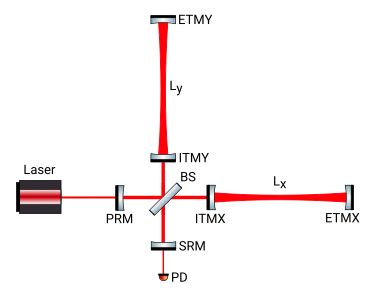
Figure 1: Schematic sketch of a general dual-recycled Fabry-Pérot-Michelson type interferometer from [30]. The assembly displayed here in depicts core features inherent to advanced LIGO [8], Virgo [9] and KAGRA [10].

To demonstrate the effects resulting from a DM-modification of the dispersion relation and to cover a larger part of the theory space, we introduce a second and third interaction types with a coupling to a photon field in QED. Concentrating on photon operators of dimension $\leq 4$ we can build an effective photon mass-term coupling via

$$\mathcal{L}_{int}\supset\frac{1}{2}m_{0}^{2}\sin^{2}\left(\frac{N_{A}\phi}{f}\right)A_{\mu}A^{\mu}$$ (13)

and an axion-like coupling,

$$\mathcal{L}_{int}\supset\frac{1}{4}\tilde{g}_{\textsc{DW}}(\phi/f)F_{\mu\nu}\tilde{F}^{\mu\nu}\;.$$ (14)

These three interactions are most commonly used in existing literature and will modify the dispersion relation of photons when applied to the QED sector. While (14) affects the fine structure constant similarly to (6), the interaction (13) does not.

We emphazise at this point that the interaction terms with impact on the fine structure constant naturally have to satisfy current experimental bounds (see [31] for the latest test). Hence, caution is necessary as for $\phi/f$ of $\mathcal{O}(1)$ this would result in a drastic change of $\alpha$ for each domain wall passing if the couplings are not fine-tuned such that the change in $\alpha$ due to a domain wall passing is within its measurement uncertainties. Alternatively, one can find an interaction for which the modification of the fine structure constant vanishes far away from the domain wall. An interaction meeting such criteria would be for instance [13]

$$\mathcal{L}_{int}\supset\frac{1}{4}g_{\textsc{DW}}\sin^{2}\left(\frac{N_{A}\phi}{f}\right)F_{\mu\nu}F^{\mu\nu}\;,$$ (15)

where using Eq. (2), the effects vanish far away from the DW as long as $N_{A}/N_{\phi}$ is integer or half integer.

Let us now consider modifications of the dispersion relation caused by interactions (6), (13) and (14). First, let us treat Eq. (13) to provide exemplary equations, and we find

$$\omega^{2}=k^{2}+m_{0}^{2}\sin^{2}\left(\frac{N_{A}\phi}{f}\right)\;,$$ (16)

such that an altered phase velocity $v_{p}=\frac{\omega}{k}$ is caused, reading

$$v_{p}=1+\frac{m_{0}^{2}}{2k^{2}}\sin^{2}\left(\frac{N_{A}\phi}{f}\right)\;,$$ (17)

and which is measurable by the interferometer. Note that (13) corresponds to an effective mass term $m_{\gamma}^{2}=m_{0}^{2}\sin^{2}\left(\frac{N_{A}\phi}{f}\right)$. It is easy to see that Eqs. (6) and (17) yield similar modifications, namely

$$\omega^{2}-k^{2}=\pm\frac{\tilde{g}_{\textsc{DW}}}{f}(\omega\partial_{t}\phi+\vec{k}\vec{\nabla}\phi)$$ (18a)

$$\omega^{2}-k^{2}=i\frac{g_{\textsc{DW}}}{f}(\omega\partial_{t}\phi^{2}+\vec{k}\vec{\nabla}\phi^{2})$$ (18b)

Note that in case of a $A_{\mu}$ being the $U(1)$ gauge potential the imaginary factor in the latter leads to an exponential power in the plane electromagnetic wave. This can be suppressed by choosing a small $g_{\textsc{DW}}$.

Starting from Eq. (17) we can now integrate over both sides such that we have

$$2L=t-t_{0}+\frac{m_{0}^{2}}{2\omega^{2}}\int_{t_{0}}^{t}\mathrm{d}t\sin^{2}\left(\frac{N_{A}\phi}{f}\right)\;,$$ (19)

where we set $c=1$. Note that we replaced $k^{2}$ with $\omega^{2}$ with respect to (17) as we expand in zeroth order in $m_{0}$ in the denominator. Note also that this formula holds for both arms equivalently. The dynamic information of the DW is solely encoded in the TDM solution $\phi$. Hence, we replace $\phi$ with $\phi\equiv\phi_{\text{TDM}}(\mathbf{x})$ where $\mathbf{x}$ contains information about the trajectory and $\phi_{\textsc{TDM}}(\mathbf{x})$ describes the extension of the DW. Outside of the DW the integrand vanishes.

Depending on its thickness and angle of impact with respect to the plane defined by the interferometer arms, the signatures of the resulting phase shift in $x$ and $y$ direction can be very distinct (we adapt the same labeling as in Figure 1). Further, we want to take into account a complete signal, i.e. we want to obtain a numerical solution for the time interval starting from $t_{0}$, where the DW does not intersect with the detector, to $t_{1}$, where the DW has passed through it.

For the general analysis we assume the spatial extent of the DW is determined by width which in turn is governed by the mass as explained above. We set the coordinate origin in our consideration to the center of our detector. For the remainder of this article we name this coordinate system the detector system (DS). Hence, the arms align with the $x$- and $y$-axis respectively. We define a vector $\mathbf{n}$ as the unit normal vector of the domain wall which characterizes the direction of motion. Typically, one assumes a velocity around $v\sim 3\cdot 10^{-3}c$. In our analysis we treat the speed as well as all other model-specific parameters as free. To determine the shape, duration and frequency of the signal produced by a modified dispersion relation, we can project the normal vector $\mathbf{n}$ onto the detector plane such the direct distance can be inserted into solution (2), i.e.

$$\tilde{\mathbf{x}}(t):=\mathbf{x}\cdot\mathbf{n}^{\textsc{DP}}-d_{0}+vt\;.$$ (20)

Here, $d_{0}$ denotes the initial distance of the DW to the detector measured normal to the plane. In turn, $\mathbf{n}_{x,y}^{\textsc{DP}}$ is the projection of the normal vector onto the detector plane which can be easily written in spherical coordinates $\mathbf{n}_{\textsc{DP}}=(\sin\theta\cos\phi,\sin\theta\sin\phi)$. See Figure 2 for a schematic sketch. The angles are given in the DS. The vector $\mathbf{x}$ labels a point in space. All in all Eq. (20) labels the distance to the domain wall of an arbitrary point $\mathbf{x}$ at time $t$. Eq. (20) can be directly inserted into (2). For our consideration we assume an infinite extension of the planar dimensions of the DW.

Let us now look at the shape of the signal. Assume we have a modification of the phase velocity by some function of the dark scalar $\phi_{\text{TDM}}$ and the photon wave vector $\mathbf{k}$, i.e.

$$v_{p}=\frac{\omega}{k}=1+\gamma(\phi_{\text{TDM}}[\tilde{\mathbf{x}}(t)],\mathbf{k})\approx 1+\gamma(\phi_{\text{TDM}}[\tilde{\mathbf{x}}(t)],\mathbf{\omega})$$ (21)

where in the last step we replaced $\mathbf{k}$ with $\omega$. The $\mathbf{k}=\omega$ approximation holds in zeroth order in $m_{0}\ll 1$. We can integrate both sides of the latter equation to find

$$N_{\text{eff}}L=t-t_{0}+\int_{t_{0}}^{t}\mathrm{d}t^{\prime}\gamma(\phi_{\text{TDM}}[\tilde{\mathbf{x}}(t^{\prime})],\mathbf{\omega})\;,$$ (22)

where $t_{0}$ is the time for which a photon emitted from the laser leaves the beam splitter for the first time and $t$ is the time when it returns from the Fabry-Pérot cavity and meets the beam splitter again. Depending on the construction of the instrument it will pass through the cavity with arm lengths $L$ roughly $N_{\text{eff}}$ - times. Hence, the factor on the left-hand-side. Based on a plane-wave representation of the photons inside the cavity we can then deduce that the phase difference in each arm is given by

$$\Delta\varphi_{x_{i}}(t)=\omega\int_{t-N_{\textsc{eff}}L}^{t}\mathrm{d}t^{\prime}\gamma(\phi_{\text{TDM}}[\tilde{x}_{x_{i}}(t^{\prime})],\mathbf{\omega})\;.$$ (23)

Note that since we aligned our coordinate system with the detector arms we can split $\tilde{\mathbf{x}}$ into its $x$ and $y$ components and completely separate Eq. (22). This results from the chosen alignment: In the reference frame $DS$, the domain wall travels with the velocity $v\ll c$ in the direction $\mathbf{n}$. Projected onto the detector plane, only the $x,y$ components of the normal vector of the domain wall are relevant, i.e. $\mathbf{n}_{\textsc{DP}}=(\sin\theta\cos\phi,\sin\theta\sin\phi)$. For an arbitrary point in space, $\mathbf{x}$, the field strengh of the TDM is given by $\phi_{\text{TDM}}(\mathbf{x}\cdot\mathbf{n}_{\textsc{DP}}-d_{0}+vt)$. In our consideration, the only relevant points in spacetime are along the detector arms which are by definition of DS aligned with the coordinate axis. Thus, calculating $\Delta\varphi$ along the $x$-axis, the $y$ component of the scalar product $\mathbf{x}\cdot\mathbf{n}^{\text{DP}}$ vanishes, and so $\tilde{x}_{x_{i}}(t^{\prime})=x_{i}n_{i}^{\text{DP}}-d_{0}+vt$.

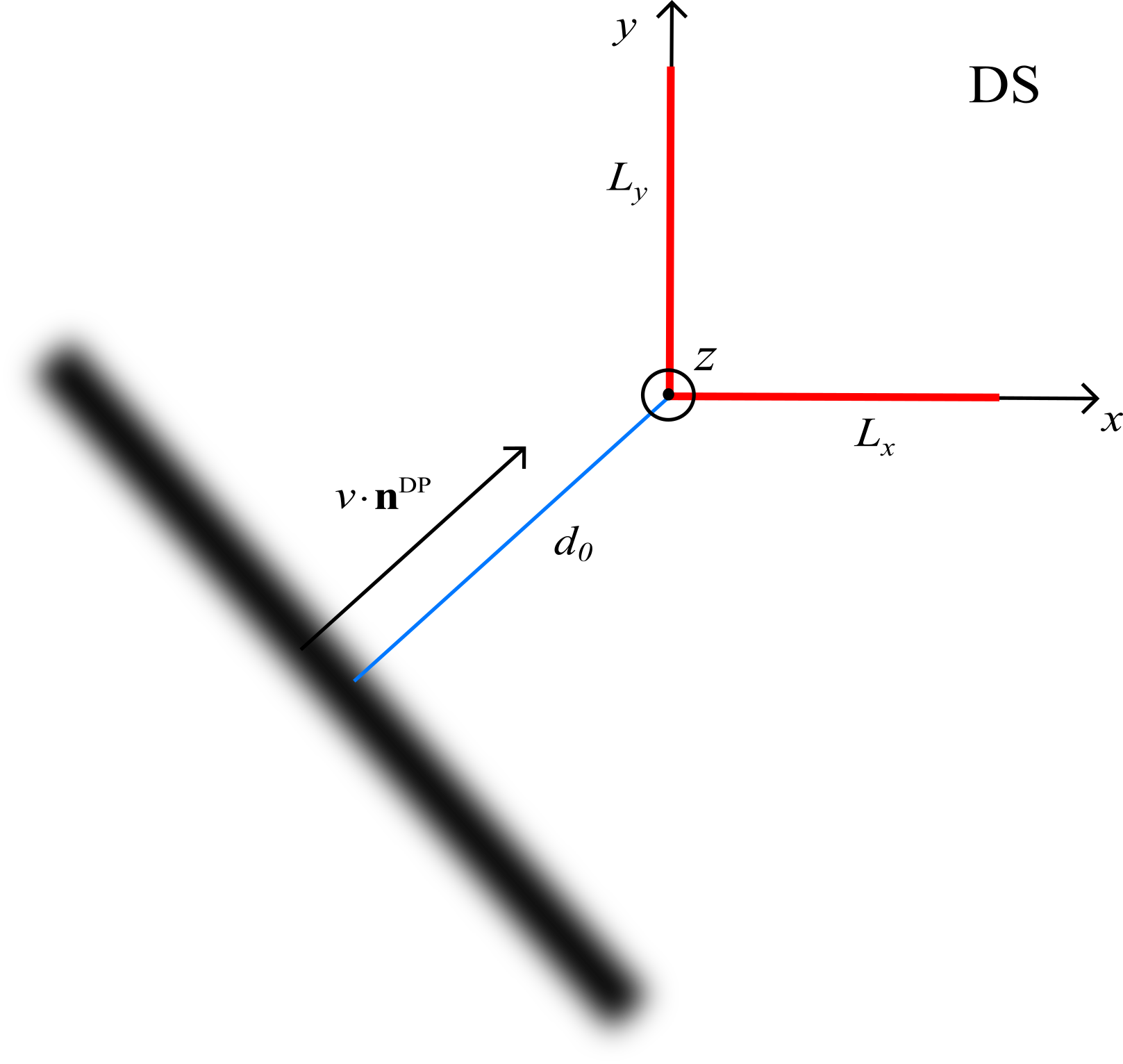
Figure 2: Two dimensional sketch of a domain wall passing through a gravitational wave interferometer. The plane resembles the detector plane with its arms aligned with the $x,y$-axis. Initial distance and velocity are given by $d_{0}$ and $v$ respectively. The vector $\mathbf{n}^{\text{DP}}$ represents the projection of the DW-normal onto the detector plane.

As mentioned before, desire to compute the phase difference between the arm since this quantity is measured in actual data. Hence, we compute

$$\Delta\varphi(t)=\Delta\varphi_{x}(t)-\Delta\varphi_{y}(t)$$ (24)

and find

$$\Delta\varphi(t)=\omega N_{\text{eff}}\left(\int_{L_{x}}\mathrm{d}x\,\gamma(\phi_{\text{TDM}}[x\sin\theta\cos\phi-d_{0}-vt])\right.\\ \left.-\int_{L_{y}}\mathrm{d}y\,\gamma(\phi_{\text{TDM}}[y\sin\theta\sin\phi-d_{0}-vt])\right)$$ (25)

As an example, consider interaction (13) where the corresponding $\gamma=\frac{m_{0}^{2}}{2\omega^{2}}\sin^{2}\left(\frac{N_{A}\phi}{f}\right)$ and upon inserting $\phi_{\textsc{TDW}}$ one finds that the phase difference measured by the interferometer is

$$\Delta\varphi(t)=\frac{m_{0}^{2}N_{\text{eff}}}{2\omega}\\ \times\left[\int_{L_{x}}\mathrm{d}x\,\sin^{2}\left(4\frac{N_{A}}{N_{\phi}}\arctan(e^{m(x\sin\theta\cos\phi-d_{0}-vt)})\right)\right.\\ -\left.\int_{L_{y}}\mathrm{d}y\,\sin^{2}\left(4\frac{N_{A}}{N_{\phi}}\arctan(e^{m(y\sin\theta\sin\phi-d_{0}-vt)})\right)\right]\;.$$ (26)

For completeness and experimental relevance let us mention that the information in frequency space can be simply extracted by Fourier transforming the latter.

To make our analysis more robust, we include a second detector. Together both detectors resemble the LIGO interferometers located in Livingston and Hanford. A DW of “infinite” planar spatial extend will inevitable introduce a phase shift $\Delta\varphi$ in both detectors. In principle, the orientation and distance of the two interferometers determines the correlation time and the shapes of the signals exactly, based on the knowledge of $\mathbf{n}$ and the DWs velocity: We lay out our coordinate system $S$ by defining a detector $A$ which we place in the origin of the coordinate grid such that the arms are aligned with the $x,y$-axis. In this frame, let $D$ be the direct distance to another coordinate system $S^{\prime}$ in whose origin the second detector $B$ is placed such that the arms again are aligned with the $x,y$-axis. Also, let $\mathbf{d}$ denote the vector connecting the origins, i.e. $\mathbf{d}=\mathbf{0}^{\prime}-\mathbf{0}$. Due to Earth’s curvature we find the two systems to be not related by translations but also rotated with respect to each other, where we define $\mathbf{R}$ to be the rotation matrix. While the signal in detector $A$ is determined by the projection of $\mathbf{n}$ onto the detector plane, i.e. the $x,y$-plane in $S$, the signal in $B$ is determined by the projection of $\mathbf{R}\mathbf{n}$ to the $x,y$-plane in $S^{\prime}$. The time in between the signals appearing in $A$ and then in $B$ or vise-versa, depends on the orientation of $\mathbf{n}$ with respect to the translation $\mathbf{d}$ connecting $S$ and $S^{\prime}$. If they are $\mathbf{d}\perp\mathbf{n}$, the signals appear in both detectors simultaneously. On the other hand if $\mathbf{d}\parallel\mathbf{n}$, the signals are correlated over a $D/v$ time interval. In between these two thresholds we expect a non-uniform random distribution of correlation times $t_{\text{corr}}\in[0,D/v]$ . Fig. 3 illustrates the positions of the two detectors.

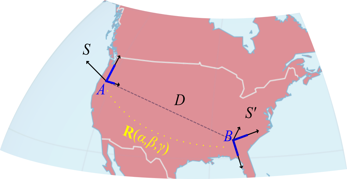
Figure 3: Sketch of the experimental setup outlined in this section. The two detectors $A,B$ are chosen to resemble the LIGO detectors on Hanford and Livingston. Note that this sketch does not respect scaling or alignment.

Let us now summarize the configuration described in this section which we use throughout the following analysis: We consider TDM in form of a DW (2) passing through Earth. Its direction and speed are given by $\mathbf{n}$ and $v$ respectively. The spatial extent of the DW perpendicular to $\mathbf{n}$ is assumed to be infinite. By passing through Earth, the DW leaves a trace in two detectors being placed on its surface at a direct distance $D$. Since the detectors arms are not aligned, the phase shifts induced by the passing DW will be of different shape and frequency, and the signals will be delayed with respect to one another. In general, the TDM within the detector yield two types of effects, a modification of the dispersion relation and a change of the optical pathway to do modified sizes of beam splitter and mirrors of the interferometer. The exact of the phase shift induced depends on the type of interaction and hence on the underlying theory.

In the following section the interaction in (15) and the resulting effects on hardware and laser propagation are analyzed numerically and compared to massive BBH events and glitches. For the remainder we stick closely to the here outlined configuration where the two detectors are assumed to be the LIGO detectors in Hanford and Livingston. Note that we do not include a third detector, i.e. Virgo [9], into our investigation as we found that for most applied cases the signal-to-noise ratio is too low to carry relevance for a potential detection of TDM, i.e. it will not affect the fitting procedure.

II.1 Sensitivity

Before moving on to the data analysis, we estimate the potential sensitivity of a search. For this we calculate the so-called 90% sensitivities for the couplings $m_{0}$ and $g_{\rm DW}$ which is a value for them that would create a signal more significant than the median of the background 90% of the time. They can also be interpreted as 90% upper limits that can be set after a search which resulted in a $p$-value of 0.5. We computed the sensitivities as a function of the scalar mass $m_{\rm dark}$ and for two example cases of $N_{\rm ratio}=N_{A}/N_{\phi}=\{2,5\}$, assuming a DW speed of $0.01c$ and considering the couplings separately. The detection statistic for significance was assumed to be the network SNR from two LIGO detectors. For each scalar mass and $N_{\rm ratio}$, we assumed a matched filtering search for that specific parameters, while searching for 400 uniformly distributed and equally separated directions in the sky. For the background, we only assumed gaussian noise at O3 sensitivity of LIGO detectors. Presence of glitches in the data may increase this sensitivity although the median of a population is generally robust against outliers therefore their effect may be minuscule. The obtained sensitivities are shown in Fig. 4. The boundaries of the scalar mass were determined by the sensitive frequency band of LIGO and the sampling rate. Lower masses would produce signals with much less frequencies going out of the band of LIGO due to the sharply increasing seismic noise below 10 Hz, where as higher masses would result in high-frequency signals which would require higher than $\gtrsim 10~{}$kHz sampling. The sensitivities for different DW speeds ($v_{\rm DW}$) can be obtained by rescaling of the parameters which satisfy the equalities

$$m_{\rm dark}v_{\rm DW}={\rm constant}_{1}$$ (27a)

$$m_{\rm dark}m_{0}^{2}={\rm constant}_{2}\ {\rm or}\ m_{\rm dark}g_{\rm DW}={\rm constant}_{2}\;.$$ (27b)

Parameters satisfying these equations would produce the same signal. We found that the sensitivities range from $\sim 10^{-9}-10^{-12}$ eV for $m_{0}$ and from $\sim 10^{-29}-10^{-16}$ for $g_{\rm DW}$ in the $m_{\rm dark}$ mass range $10^{-12}-10^{-10}$ eV for $v_{\rm DW}=0.01c$.

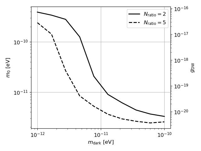
Figure 4: 90% sensitivities of the couplings as a function of the scalar mass and the $N_{\rm ratio}$ parameter for $v_{\rm DW}=0.01c$

III Analysis

Here with numerical examples we investigate the presence of TDM in GW data. First we question whether some of the detected BBH mergers could also be explained by TDM. We specifically concentrate to the events which were estimated to have high detector frame black hole masses; since their signal durations are short within the sensitive frequency band of the detectors. Hence, they do not clearly show the complete inspiral-merger-ringdown waveform of a merging binary. We investigate whether their observed signals which can be explained by the last moments of a compact binary coalescence (CBC) can also be explained by a passing TDM. However, this analysis inevitably has a negative selection bias for testing the TDM scenario, as these events were found by template based searches which uses BBH waveforms. Therefore they are expected to be similar to BBH waveforms beforehand. However, we do this study as the first analysis testing presence of TDM signals in the data. A proper search for it would require a specifically designed pipeline which is discussed in Sec. IV. Second, we examine the similarity between the TDM signals and the noise artifacts in the data known as glitches. This second part serves as an exploratory analysis for a TDM search within the GW data, as TDM waveforms similar to glitches could be easily discarded, making their discovery harder.

III.1 TDM as BBH events

There are two types of searches that may detect BBH mergers: template based searches and unmodelled burst searches. Template based searches assume a compact binary coalescence (CBC) scenario and performs a matched filtering search using the gravitational waveforms for CBCs. On the other hand, in general, burst searches do not assume an astrophysical scenario and searches for a coherent excess power between different GW detectors. At the end of three observing runs of Advanced LIGO and Advanced Virgo detectors there have been about 90 confident mergers detected. All of these were found by the template based pipelines, meaning they are all interpreted as CBC mergers. Some of them were also found by the burst searches.

Although the signals of these detections could be explained by CBC waveforms, the parameters of some of them were astrophysically unexpected and they challenged our astrophysical stellar evolution models. One of the first and most drastic example of such an event was GW190521 [32]. Being a confident detection found by both the CBC and burst pipelines, both of its component BHs were estimated to be most likely to be above 50 M_⊙, lying in the so-called upper mass gap or the pair-instability mass gap where no compact object is expected from stellar evolution due to the pair-instability supernova phenomenon. Alternative explanations for its origin or properties have been proposed; such as hierarchical mergers [33, 34, 35], eccentric merger [36, 37, 38] or components with exotic matter [39, 40]. One scenario eliminated in the original analysis was a GW signal from cosmic strings instead of a BBH merger [41].

One reason of having such many possible explanations is the short signal duration observed. Being a heavy mass BBH merger, only the last few cycles of the merger were observable in the sensitive frequency range of LIGO and Virgo. This property also motivates this part of our study. Interaction of TDM with the GW detectors can also generate similar signals to the ones observed. A similarity can be expected when a chirp-like evolution is not very clear as TDM signals are symmetric in time unlike chirps; their frequency increases and then decreases in time. This trial of an alternative explanation is substantially different than slightly modified merger scenarios such as an eccentric merger or merger of Proca stars. We used 8 parameters ($\bm{\theta}$) in our model. These are the 3-D velocity vector of the TDM, a reference time for the signal (equivalent to the distance to the TDM at a reference time) and the 4 parameters that enter the interaction Lagrangian which we introduced earlier: $m_{\rm dark}$, $m_{0}$, $N_{\rm ratio}$, $g_{\rm DW}$. We parametrized the 3-D velocity vector with its speed magnitude, cosine of its zenith angle with respect to the Hanford detector and its azimuth angle with respect to the X-arm of the Hanford detector. The CBC signals were paramterized with the 15 parameters: the total detector frame mass of BHs, their mass ratio, their dimensionless 3-D spin vectors with respect to the orbital momentum, cosine of the inclination of the orbital plane with the line of sight, coalescence phase, cosine of declination, right ascension, luminosity distance to source, detection time and the polarization angle of the GW vector.

We have chosen 4 confident detections to analyze which have estimated high masses and do not show a clear chirp in their time-frequency plots to human eye, as expected from CBCs: GW190426_190642, GW190521, GW191109_010717 and GW200220_061928. We further analyzed the marginal intermediate mass black hole triggers 200114_020818 and 200214_224526. We used the 32 s long data segments from LIGO Hanford and LIGO Livingston detectors around the events sampled at 4096 Hz from the Gravitational Wave Open Science Center (https://gwosc.org) [42]. We did not use the data from Virgo even when it is available due to its lesser sensitivity which would not change our results qualitatively. To reduce the computing expense of these events with low-frequency ”signals”, we down-sampled the data to 409.6 Hz after filtering with an ideal low-pass filter at the half sampling frequency. We whitened the data by obtaining the noise power spectral density via Welch’s average periodogram method with segment lengths of 512, using the matplotlib python package’s matplotlib.pyplot.psd function [43]. We performed parameter estimations for the TDM scenario using our model and the BBH scenario using the NRSur7dq4 waveforms [44] via the gwsurrogate package [45]. For sampling, we used the dynesty sampler [46] under the Bilby framework [47, 48]. We note that our sampling is probably not optimal for finding global fits and can be stuck at locally good parts of the parameter space.

For comparing hypotheses ($H$), we rely on the Bayesian evidence ($\mathcal{B}$) or the marginal likelihood

$$\mathcal{B}(H)=\int\mathcal{L}(\bm{\theta}|H)P(\bm{\theta}|H)d\bm{\theta}\;,$$ (28)

where $P(\bm{\theta})$ is the prior distribution of the parameters and the likelihood $\mathcal{L}$ is calculated with the residual signal after the model ($h$) is subtracted from the data ($d$) by assuming a Gaussian noise. We used uniform prior distributions for our parameters, which have been parameterized appropriately for corresponding to isotropic orientations and distributions in space, except the distance prior which we take proportional to distance squared. For whitened data, up to a constant, the logarithm of the likelihood is

$$\ln\mathcal{L}=-\frac{1}{2}\langle d-h(\bm{\theta})|d-h(\bm{\theta})\rangle\;,$$ (29)

where the brackets denote the inner product of vectors. The joint likelihood from two detectors is simply the product of individual likelihoods.

Analysis on all the CBC events favored the BBH scenario over the TDM scenario. Here we only elaborate on the event which produced the best fits: GW190521. We consider the signal around 200214_224526 in the next subsection as an example of a glitch trigger. The closest case was of GW190521 with an log-evidence difference of $\Delta\ln\mathcal{B}\approx 18$ favoring the BBH scenario. In Fig. 5 we show the best fitting BBH and TDM templates to the data of Hanford and Livingston. The log-likelihood difference for these two cases is about $\Delta\ln\mathcal{L}\approx 25$ favoring the BBH fit. The TDM fits were first done without the $g_{\rm DW}$ term for this event. We observed that the addition of it to the modelling does not improve the fit meaningfully. Hence we show the results without it for GW190521. The parameter estimations for the TDM and BBH scenarios are shown in Figs. 6 and 7 respectively. Although Fig. 5 shows similar fits for both hypotheses, there is a small phase evolution difference between them which makes the BBH fit better. In Fig. 6, the TDM fits have very precise estimation for the orientation of the DW. This is due to the 2-3 orders of magnitude smaller speed of the DW than GWs. Therefore the time delay of the signals between the detectors can be achieved only within a small parameter volume, which could be more easily achieved with a propagation at the speed of light. As the second best one, for comparison, we only show the fits for the event GW191109_010717 in Fig. 8.

Finally, due to the good fits we got with the TDM model to the BBH mergers we fit BBH templates to the best fitting TDM template for GW190521. This was done to understand whether BBH searches can detect TDM signals. We found that the signal-to-noise ratio (SNR) of the best fitting BBH template to the TDM signal is about $\sim$90% of the actual SNR of the TDM signal which means that the template based BBH searches can catch some of TDM signals.

Figure 5: Whitened best fitting TDM and BBH signals on the data of GW190521

Figure 6: Parameter estimation of the TDM scenario for the GW190521. $m_{\rm dark}$ and $m_{0}$ in units of $10^{-12}$ eV, $v_{\rm DW}$ in units of $c$, det-t in seconds and phi-LHO in radians. The estimated $N_{\rm ratio}$ is 3.

Figure 7: Parameter estimation of the BBH scenario for the GW190521. Parameters respectively are total mass in detector frame [$M_{\odot}$], mass ratio$\geq 1$, magnitudes and angular orientations of the dimensionless spins, cosine of the orbital inclination, coalescence phase, right ascension, cosine of declination, luminosity distance [Mpc], reference detection time [s] and polarization angle. Angular quantities are in radians and definitions of the spin orientations are according to the assumed coordinate system of the gwsurrogate package [45].

Figure 8: Whitened best fitting TDM and BBH signals on the data of GW191109_010717

III.2 TDM as Glitches

The LIGO detectors are frequently plagued by glitches, that are reoccurring signatures in the data which cannot be assigned to astrophysical sources. Despite their failure to match merger events, glitches play an important role in the data analysis challenges creating false alarms. By today more than twenty distinct glitch types have been classified and large efforts are brought up to investigate their origin. While the sources of some of them have been identified, some are still not fully understood. Here, we investigate whether glitches can limit TDM searches in the GW detector data. We consider two cases: first we examine the possible effects of the ”blip” glitches, second we analyze a fast scattering glitch around the 200214_224526 trigger.

III.2.1 Blip glitches

Here we focus on one particular family of glitches, the so called “blips”, identified by their characteristic shape in the time-frequency plane. TDM signals can be very similar to blips if the DWs traverses an interferometer arm perpendicularly, creating a very short signal. In Fig. 9 we display a blip and a similarly looking signal from TDM to motivate our choice of glitch we aim to match to TDM. The top panel shows a piece of actual data of the Hanford detector in which a blip appears, where as the bottom displays the spectrogram for a TDM within some noisy background with sufficiently high signal-to-noise ratio. Despite there being many more glitches that have not yet been assigned to a particular phenomenology, we find the blip-type glitches to be the only ones exhibiting adequate similarities.

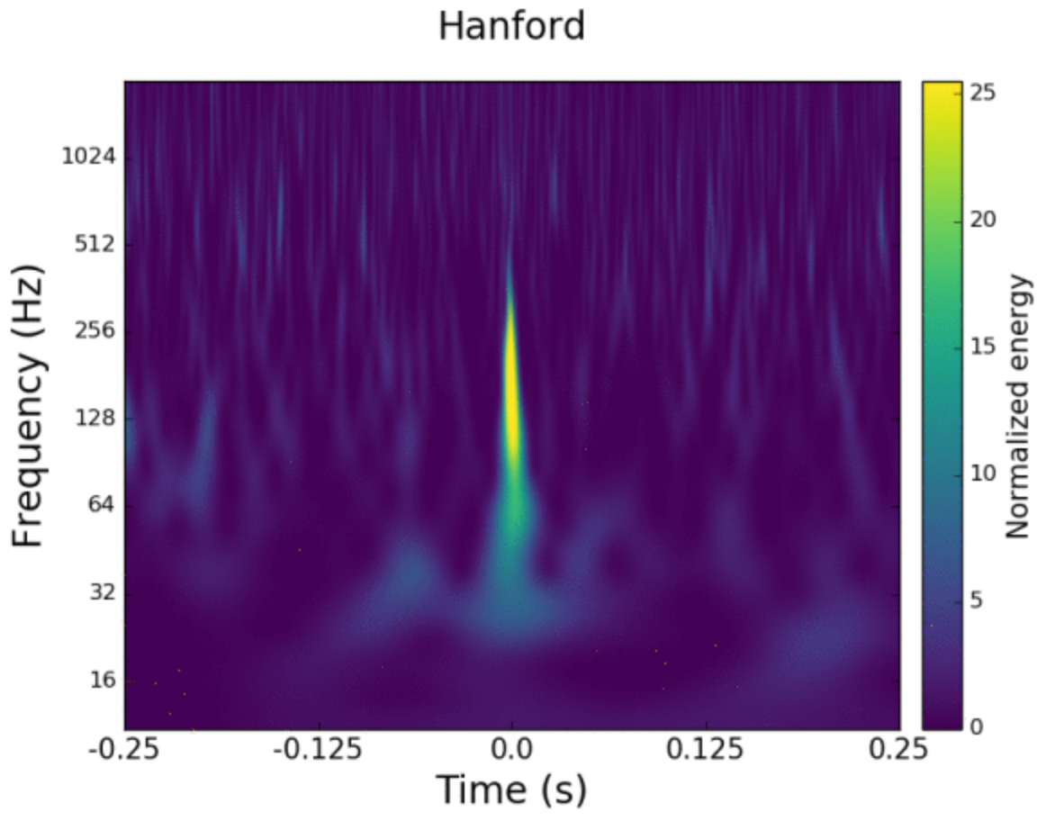
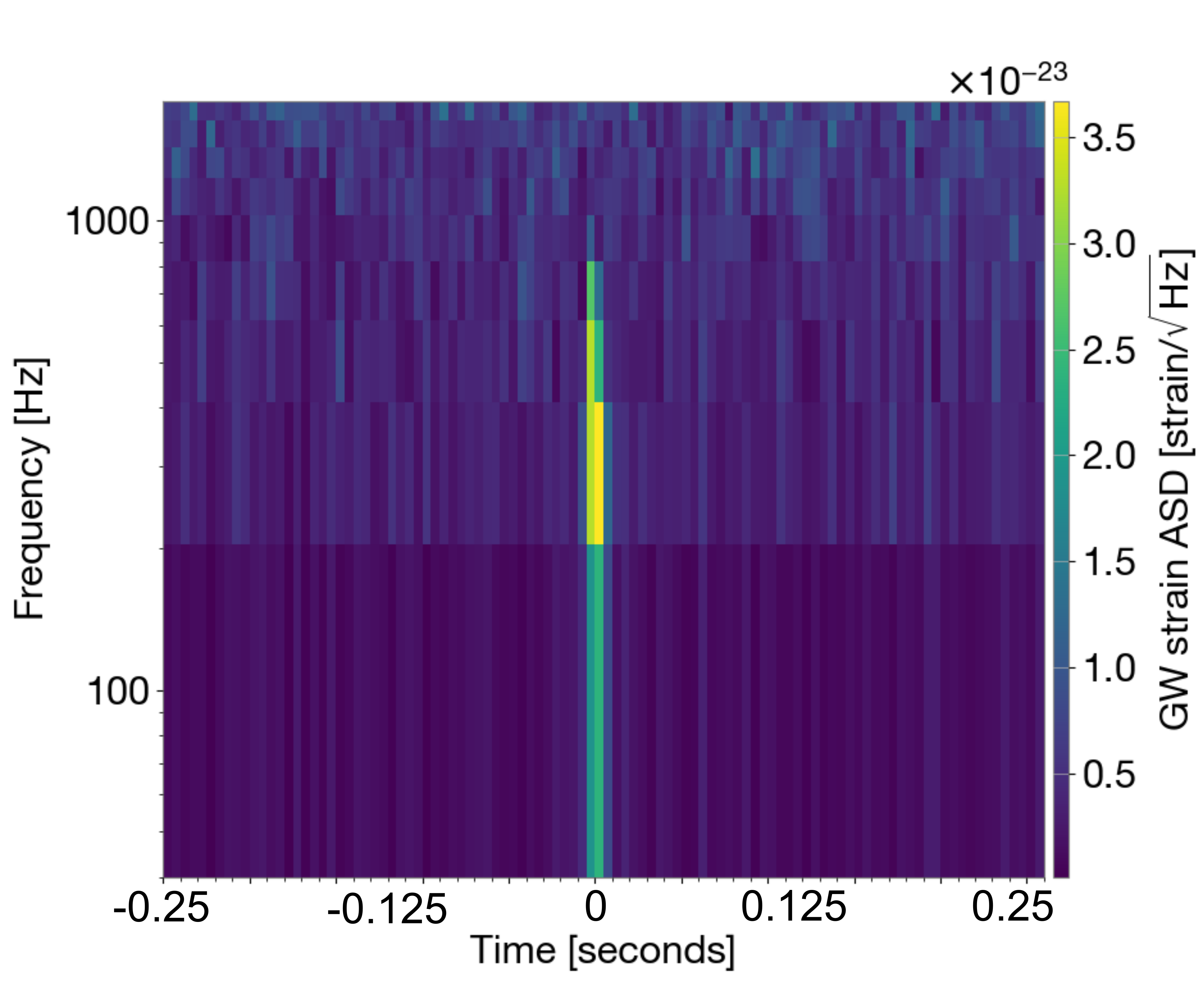
Figure 9: Spectograms of (top) an exemplary blip glitch recorded in the Hanford detector (from GravitySpy collection [49, 50]) and (bottom) a TDM signal simulated with some background noise.

Blips appear in LIGO detectors’ data of a rate about a few per hour [51], allowing the cases where they can appear in both LIGO detectors with only a few fractions of a second delay during the year-long observing runs. Hence, they embody a suitable systematic effect for TDM searches. This is more severe than the GW searches as the allowed time delay between the detectors can be 2-3 orders of magnitude larger than the GW searches due to slower expected propagation speeds of DWs. To investigate the possible effect of blips to TDM searches, we compared multiple realizations of blips with the signatures produced by TDM in a realistic setup. To have variety of blip signals, and not to search them in real data, we used the glitch generator empowered with machine learning [52].

As in the previous subsection, we adapted the setup outlined in Sec. II to our needs, i.e. we placed the glitch in the detector data at a given $t_{0}$. We then simulated the DW of TDM passing through the detector such that the signal appears at $t_{0}$ as well. Again, we applied a similar sampling scheme to find the best fit for the model parameters $m_{\text{dark}},m_{0},v,N_{A}/N_{\phi},\theta,\phi$ where the latter angles parameterize the projection of the DWs unit normal vector $\mathbf{n}$ onto the detector plane. Prior to the evaluation of the likelihood, glitch and TDM signals were whitened. We did not perform a joint analysis between the detectors and considered the fits to individual glitches. The effects on beam splitter and mirrors, in Eq. (12), are subdominant in the glitch analysis and hence irrelevant for our proof of principle. We display two exemplary fits in Figure 10. The simulations displayed here are resulting from multiple runs of the sampling scheme where after each run we adapt the priors to narrow down the desired domain for each parameter ultimately resulting in a better fit. We found that the glitches resemble TDM signals with specific parameters. Concretely, we find that $m_{\text{dark}}\sim 2\cdot 10^{-12}$ eV, $m_{0}\sim 10^{-11}$ eV, $N_{A}/N_{\phi}=2$, $v\sim 10^{-2}\cdot c$ consistently for all fits. We note that these parameter values are astrophysically relevant as they satisfy the regularity conditions calculated in Sec. I regarding the DW crossings per unit time. However, due to the uncorrelated nature of glitches between detectors, they cannot be explained by TDM. In the signals, $m_{0}$ mainly influences the amplitude of the phase difference induced by the DW, $m_{\text{dark}},v$ result in squeezing and stretching along the $x$-axis. The fraction $N_{A}/N_{\phi}$ roughly monitors the number of peaks. It is the most susceptible to the glitch realization.

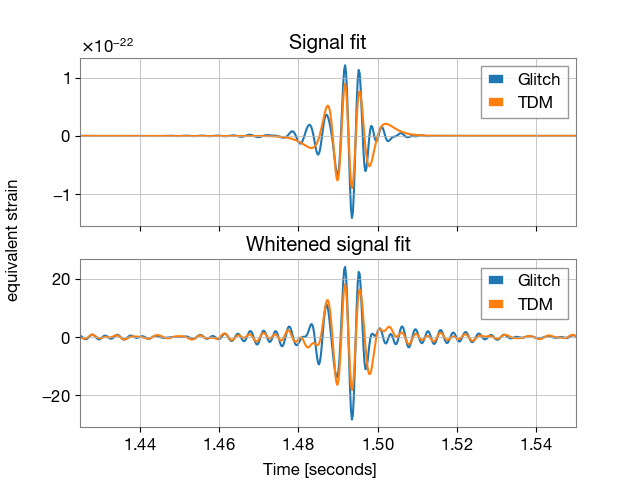
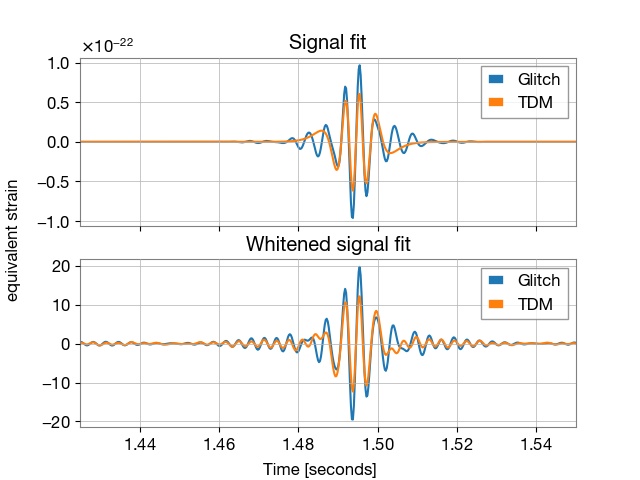
Figure 10: Fits for simulated TDM signatures inside Livingston onto blip-glitches generated by the GlitchGen AI tool [52].

Note that while we show only blips fitted to DW signals, we investigated for other glitch types as well. After a pre-selection based on their shape in frequency space we narrowed the suitable types down to blips and tomtes (the latter displayed in Figure 11). While there are similarities regarding the general shape of the signal, the power in the lower frequency regime is spread out significantly more than what is achievable with TDM. Hence, we discard tomtes as potential systematics caused by TDM passing through Earth gravitational wave detectors.

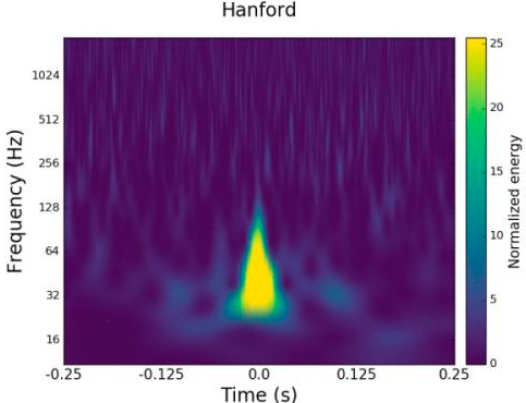
Figure 11: Example of a Tomte-type glitch (from GravitySpy collection [49, 50])

In conclusion, in this chapter we gather more evidence that DW of TDM can be probed with gravitational interferometers. Additionally to the previously in Sec. III.1 outlined analysis regarding the match of TDM signatures to pre-selected BBH events, we show that there are reappearing glitches within the actual LIGO data matching the time-frequency profile of TDM for a limited part of the parameter space. The fits are robust against noise and expected to appear frequent enough to test for correlations amongst both LIGO detectors. The latter is left to future work on actual data.

III.2.2 Fast scattering glitch

While analyzing the BBH events, we also analyzed the marginal intermediate mass black hole triggers. Among them we noticed that the fast scattering glitch in Livingston which causes the 200214_224526 trigger can also be fitted by the TDM signal. The fast scattering glitch has the characteristic of repeated bursts. In this trigger, we analyzed the most powerful two bursts. We applied the same analysis with the BBH analysis in Sec. III.1, analyzing both detectors jointly. In Fig. 12 we show the data of the detectors and the fitting TDM templates.

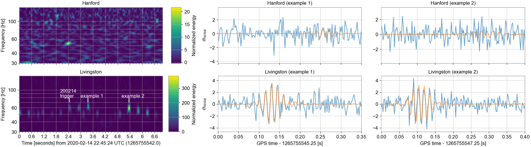
Figure 12: (Left) Q-transforms of the (top row) Hanford and (botom row) Livingston data around the 200214_224526 trigger. (Middle and Right) the detector data in blue and the TDM signal fit in orange for the most powerful bursts of the glitch (pointed in the left bottom)

IV Discussion

In this article, we investigated the detectability of TDM with the gravitational wave interferometers and conducted a partial analysis on the data of LIGO searching for TDM signals. First of all, our findings showed that although having a very different physical motivation and having much less parameters in the modelling compared to CBC sources (8 vs. 15), TDM signals can look like BBH mergers. Specifically, we found that the GW190521 event can also be explainable with the TDM hypothesis although it is not favored against the BBH explanation. Furthermore we found that CBC searches can catch TDM signals. In our example, a BBH template was able to produce $\sim$90% of the actual SNR of the best fitting TDM template to GW190521. Since this is just one example, the detectability of TDM signals with different parameters can be more or less feasible than this.

Second, we also found that the TDM signals and glitches in the data can have similarities. We found that the blip glitches look like a TDM signal with particular parameters ($m_{\text{dark}}\sim 2\cdot 10^{-12}$ eV, $m_{0}\sim 10^{-11}$ eV, $N_{A}/N_{\phi}=2$, $v\sim 10^{-2}\cdot c$) meaning identification of a TDM signal with these parameters could be obscured by the presence of blip glitches. We also found that different kinds of glitches can also be problematic. The TDM model was able to fit a fast scattering glitch. These results point out possible systematic issues for TDM searches in the GW data.

Now, we discuss the modifications that needs to be done to the GW searches in order to search for TDM signals. The most straightforward change is the expansion of the detection delay time window between detectors due to the slow speeds of DWs. The expected speeds of them could be as low as $10^{-3}c$ which requires much longer time windows to be used. This will inevitably result in a less powerful search due to the increased number of expected noise triggers in the time window. The second modification that needs to be done is elimination of assumptions about GW polarizations in the pipelines. Both the CBC and unmodelled burst pipelines assumes a transformation of the signal between the detectors based on the polarization of the GWs. This transformation should be abandoned or modified according to the two possible and independent effects of the TDM (i) on the phase velocity of light, e.g., Eq. (26) (ii) on the fine structure constant, e.g., Eq. (12). Moreover, the antenna patterns of the detectors should be modified (i) due to the narrow physical thickness of the DW compared to the GW wavelength which cannot be assumed to be in the long ”wavelength” limit (ii) and also due to the different way of producing a signal in the interferometer with the changing fine structure constant (the changing phase velocity of light and the effect of GWs on distances are equivalent to each other in different reference frames).

References

- Feng [2010] J. L. Feng, Annual Review of Astronomy and Astrophysics 48, 495 (2010), https://doi.org/10.1146/annurev-astro-082708-101659 .
- Arbey and Mahmoudi [2021] A. Arbey and F. Mahmoudi, Progress in Particle and Nuclear Physics 119, 103865 (2021).
- Khoury [2015] J. Khoury, A dark matter superfluid (2015), arXiv:1507.03013 [astro-ph.CO] .
- Adams et al. [2023] C. B. Adams, N. Aggarwal, A. Agrawal, R. Balafendiev, C. Bartram, M. Baryakhtar, H. Bekker, P. Belov, K. K. Berggren, A. Berlin, et al., Axion dark matter (2023), arXiv:2203.14923 [hep-ex] .
- Flambaum and Stadnik [2023] V. Flambaum and Y. Stadnik, in Springer Handbook of Atomic, Molecular, and Optical Physics (Springer International Publishing, 2023) pp. 461–469.
- Safronova et al. [2018] M. S. Safronova, D. Budker, D. DeMille, D. F. J. Kimball, A. Derevianko, and C. W. Clark, Rev. Mod. Phys. 90, 025008 (2018).
- Derevianko and Pospelov [2014] A. Derevianko and M. Pospelov, Nature Physics 10, 933 (2014).
- Aasi et al. [2015] J. Aasi, B. P. Abbott, R. Abbott, T. Abbott, M. R. Abernathy, K. Ackley, C. Adams, T. Adams, P. Addesso, R. X. Adhikari, et al., Classical and Quantum Gravity 32, 074001 (2015).
- Acernese et al. [2015] F. Acernese, M. Agathos, K. Agatsuma, D. Aisa, N. Allemandou, A. Allocca, J. Amarni, P. Astone, G. Balestri, G. Ballardin, et al., Classical and Quantum Gravity 32, 024001 (2015), arXiv:1408.3978 [gr-qc] .
- Akutsu et al. [2020] T. Akutsu, M. Ando, K. Arai, Y. Arai, S. Araki, A. Araya, N. Aritomi, Y. Aso, S. Bae, Y. Bae, L. Baiotti, R. Bajpai, M. A. Barton, et al., Progress of Theoretical and Experimental Physics 2021, 05A101 (2020), https://academic.oup.com/ptep/article-pdf/2021/5/05A101/37974994/ptaa125.pdf .
- Jaeckel et al. [2016] J. Jaeckel, V. V. Khoze, and M. Spannowsky, Physical Review D 94, 10.1103/physrevd.94.103519 (2016).
- Grote and Stadnik [2019a] H. Grote and Y. V. Stadnik, Phys. Rev. Res. 1, 033187 (2019a).
- Khoze and Milne [2022] V. V. Khoze and D. L. Milne, Physics Letters B 829, 137044 (2022).
- Pospelov et al. [2013] M. Pospelov, S. Pustelny, M. P. Ledbetter, D. F. J. Kimball, W. Gawlik, and D. Budker, Phys. Rev. Lett. 110, 021803 (2013).
- Vermeulen et al. [2021] S. M. Vermeulen, P. Relton, H. Grote, V. Raymond, C. Affeldt, F. Bergamin, A. Bisht, M. Brinkmann, K. Danzmann, S. Doravari, V. Kringel, J. Lough, H. Lück, M. Mehmet, N. Mukund, S. Nadji, E. Schreiber, B. Sorazu, K. A. Strain, H. Vahlbruch, M. Weinert, B. Willke, and H. Wittel, Nature 600, 424 (2021).
- Pierce et al. [2018] A. Pierce, K. Riles, and Y. Zhao, Physical Review Letters 121, 10.1103/physrevlett.121.061102 (2018).
- Guo et al. [2019] H.-K. Guo, K. Riles, F.-W. Yang, and Y. Zhao, Communications Physics 2, 10.1038/s42005-019-0255-0 (2019).
- Abbott et al. [2022] R. Abbott, T. Abbott, F. Acernese, K. Ackley, C. Adams, N. Adhikari, R. Adhikari, V. Adya, C. Affeldt, D. Agarwal, M. Agathos, et al., Physical Review D 105, 10.1103/physrevd.105.063030 (2022).
- Afach et al. [2021] S. Afach, B. C. Buchler, D. Budker, C. Dailey, A. Derevianko, et al., Nature Physics 17, 1396 (2021).
- Wcisło et al. [2018] P. Wcisło, P. Ablewski, K. Beloy, S. Bilicki, M. Bober, et al., Science Advances 4, eaau4869 (2018), https://www.science.org/doi/pdf/10.1126/sciadv.aau4869 .
- Roberts et al. [2017] B. M. Roberts, G. Blewitt, C. Dailey, M. Murphy, M. Pospelov, A. Rollings, J. Sherman, W. Williams, and A. Derevianko, Nature Communications 8, 10.1038/s41467-017-01440-4 (2017).
- Stadnik [2020] Y. V. Stadnik, Phys. Rev. D 102, 115016 (2020).
- Yang et al. [2021] Y. Yang, T. Wu, J. Zhang, and H. Guo, Chinese Physics B 30, 050704 (2021).
- Roberts et al. [2020] B. M. Roberts, P. Delva, A. Al-Masoudi, A. Amy-Klein, C. Bærentsen, C. F. A. Baynham, E. Benkler, S. Bilicki, S. Bize, W. Bowden, et al., New Journal of Physics 22, 093010 (2020).
- Sikivie [1982] P. Sikivie, Phys. Rev. Lett. 48, 1156 (1982).
- Kawasaki et al. [2015] M. Kawasaki, K. Saikawa, and T. Sekiguchi, Physical Review D 91, 10.1103/physrevd.91.065014 (2015).
- Avelino et al. [2008] P. P. Avelino, C. J. A. P. Martins, J. Menezes, R. Menezes, and J. C. R. E. Oliveira, Phys. Rev. D 78, 103508 (2008).
- Friedland et al. [2003] A. Friedland, H. Murayama, and M. Perelstein, Phys. Rev. D 67, 043519 (2003).
- Tanabashi et al. [2018] M. Tanabashi, K. Hagiwara, K. Hikasa, K. Nakamura, Y. Sumino, F. Takahashi, J. Tanaka, K. Agashe, G. Aielli, C. Amsler, et al. (Particle Data Group), Phys. Rev. D 98, 030001 (2018).
- Grote and Stadnik [2019b] H. Grote and Y. V. Stadnik, Physical Review Research 1, 10.1103/physrevresearch.1.033187 (2019b).
- Shuvaev et al. [2022] A. Shuvaev, L. Pan, L. Tai, P. Zhang, K. L. Wang, and A. Pimenov, Applied Physics Letters 121, 193101 (2022), https://pubs.aip.org/aip/apl/article-pdf/doi/10.1063/5.0105159/16487755/193101_1_online.pdf .
- Abbott et al. [2020a] R. Abbott, T. D. Abbott, S. Abraham, F. Acernese, K. Ackley, C. Adams, R. X. Adhikari, et al. (LIGO Scientific Collaboration and Virgo Collaboration), Phys. Rev. Lett. 125, 101102 (2020a).
- Veske et al. [2021] D. Veske, A. G. Sullivan, Z. Márka, I. Bartos, K. R. Corley, J. Samsing, R. Buscicchio, and S. Márka, The Astrophysical Journal 907, L48 (2021).
- Kimball et al. [2021] C. Kimball, C. Talbot, C. P. L. Berry, M. Zevin, E. Thrane, V. Kalogera, R. Buscicchio, M. Carney, T. Dent, H. Middleton, E. Payne, J. Veitch, and D. Williams, The Astrophysical Journal 915, L35 (2021).
- Tagawa et al. [2021] H. Tagawa, B. Kocsis, Z. Haiman, I. Bartos, K. Omukai, and J. Samsing, The Astrophysical Journal 908, 194 (2021).
- Romero-Shaw et al. [2020] I. Romero-Shaw, P. D. Lasky, E. Thrane, and J. C. Bustillo, The Astrophysical Journal 903, L5 (2020).
- Gamba et al. [2023] R. Gamba, M. Breschi, G. Carullo, S. Albanesi, P. Rettegno, S. Bernuzzi, and A. Nagar, Nature Astronomy 7, 11 (2023).
- Gayathri et al. [2022] V. Gayathri, J. Healy, J. Lange, B. O’Brien, M. Szczepańczyk, I. Bartos, M. Campanelli, S. Klimenko, C. Lousto, and R. O’Shaughnessy, Nature Astronomy 6, 344 (2022).
- Bustillo et al. [2021] J. C. Bustillo, N. Sanchis-Gual, A. Torres-Forné, J. A. Font, A. Vajpeyi, R. Smith, C. Herdeiro, E. Radu, and S. H. W. Leong, Phys. Rev. Lett. 126, 081101 (2021).
- Bustillo et al. [2022] J. C. Bustillo, N. Sanchis-Gual, S. H. W. Leong, K. Chandra, A. Torres-Forne, J. A. Font, C. Herdeiro, E. Radu, I. C. F. Wong, and T. G. F. Li, Searching for vector boson-star mergers within ligo-virgo intermediate-mass black-hole merger candidates (2022), arXiv:2206.02551 [gr-qc] .
- Abbott et al. [2020b] R. Abbott, T. D. Abbott, S. Abraham, F. Acernese, K. Ackley, C. Adams, R. X. Adhikari, et al., The Astrophysical Journal Letters 900, L13 (2020b).
- Abbott et al. [2023] R. Abbott, H. Abe, F. Acernese, K. Ackley, S. Adhicary, N. Adhikari, R. X. Adhikari, V. K. Adkins, V. B. Adya, C. Affeldt, D. Agarwal, M. Agathos, O. D. Aguiar, et al., The Astrophysical Journal Supplement Series 267, 29 (2023).
- Hunter [2007] J. D. Hunter, Computing in Science and Engineering 9, 90 (2007).
- Varma et al. [2019] V. Varma, S. E. Field, M. A. Scheel, J. Blackman, D. Gerosa, L. C. Stein, L. E. Kidder, and H. P. Pfeiffer, Physical Review Research 1, 10.1103/physrevresearch.1.033015 (2019).
- Field et al. [2014] S. E. Field, C. R. Galley, J. S. Hesthaven, J. Kaye, and M. Tiglio, Physical Review X 4, 031006 (2014), arXiv:1308.3565 [gr-qc] .
- Speagle [2020] J. S. Speagle, Monthly Notices of the Royal Astronomical Society 493, 3132 (2020).
- Ashton et al. [2019] G. Ashton, M. Hübner, P. D. Lasky, C. Talbot, K. Ackley, S. Biscoveanu, Q. Chu, A. Divakarla, P. J. Easter, B. Goncharov, et al., The Astrophysical Journal Supplement Series 241, 27 (2019), arXiv:1811.02042 [astro-ph.IM] .
- Romero-Shaw et al. [2020] I. M. Romero-Shaw, C. Talbot, S. Biscoveanu, V. D’Emilio, G. Ashton, C. P. L. Berry, S. Coughlin, S. Galaudage, C. Hoy, M. Hübner, et al., Monthly Notices of Royal Astronomical Society 499, 3295 (2020), arXiv:2006.00714 [astro-ph.IM] .
- [49] Gravityspy webpage, https://www.zooniverse.org/projects/zooniverse/gravity-spy.
- Zevin et al. [2017] M. Zevin, S. Coughlin, S. Bahaadini, E. Besler, N. Rohani, S. Allen, M. Cabero, K. Crowston, A. K. Katsaggelos, S. L. Larson, et al., Classical and Quantum Gravity 34, 064003 (2017).
- Cabero et al. [2019] M. Cabero, A. Lundgren, A. H. Nitz, T. Dent, D. Barker, E. Goetz, J. S. Kissel, L. K. Nuttall, P. Schale, R. Schofield, and D. Davis, Classical and Quantum Gravity 36, 155010 (2019).
- Powell et al. [2023] J. Powell, L. Sun, K. Gereb, P. D. Lasky, and M. Dollmann, Classical and Quantum Gravity 40, 035006 (2023).