RCCZ4: A Reference Metric Approach to Z4

Abstract

The hyperbolic formulations of numerical relativity due to Baumgarte, Shapiro, Shibata & Nakamura (BSSN) and Nagy Ortiz & Reula (NOR), among others, achieve stability through the effective embedding of general relativity within the larger Z4 system. In doing so, various elliptic constraints are promoted to dynamical degrees of freedom, permitting the advection of constraint violating modes. Here we demonstrate that it is possible to achieve equivalent performance through a modification of fully covariant and conformal Z4 (FCCZ4) wherein constraint violations are coupled to a reference metric completely independently of the physical metric. We show that this approach works in the presence of black holes and holds up robustly in a variety of spherically symmetric simulations including the critical collapse of a scalar field. We then demonstrate that our formulation is strongly hyperbolic through the use of a pseudodifferential first order reduction and compare its hyperbolicity properties to those of FCCZ4 and generalized BSSN (GBSSN).

Our present approach makes use of a static Lorentzian reference metric and does not appear to provide significant advantages over FCCZ4. However, we speculate that dynamical specification of the reference metric may provide a means of exerting greater control over constraint violations than what is provided by current BSSN-type formulations.

I Introduction

The formulations of numerical relativity based on the Baumgarte, Shapiro, Shibata & Nakamura (BSSN) decomposition effectively achieve strong hyperbolicity and stability by performing a partial embedding of general relativity (GR) within the larger Z4 system [1, 2, 3]. In this paper we demonstrate that the Z4 system is not uniquely suitable for this purpose and present an alternative formulation of GR that is also well suited for numerical relativity. This formulation is based on an alternative embedding of GR and holds up well in a variety of simulations in spherical symmetry including those of black holes with puncture initial data as well as in the critical collapse of the massless scalar field. Additionally, we show that our new formulation is strongly hyperbolic and, in fact, has the same principal symbol as fully covariant and conformal Z4 (FCCZ4).

The Z4 formulation takes its name from the introduction of a four vector, $Z_{\mu}$, to the Einstein equations,

$$R_{\mu\nu}+2\nabla_{(\mu}Z_{\nu)}-8\pi\left(T_{\mu\nu}-\frac{1}{2}g_{\mu\nu}T\right) =0.$$ (1)

In the context of general relativity, the evolution of this system acts to advect and/or damp violations of the Hamiltonian and momentum constraints. In the limit $Z_{\mu}\rightarrow 0$ we recover GR [4].

If we examine formulations such as NOR [5] and generalized BSSN (GBSSN) [6] in detail, we find that they are essentially minor variations of Z4-derivable formulations in which the temporal component of $Z_{\mu}$ is not evolved and substitutions or additions of the Hamiltonian and momentum constraints have been made [1, 2, 7, 3, 8, 9]. The case could also be made that the equations of motion of Z4 formalisms arise naturally while those of NOR and GBSSN come from experimentation to achieve stability and strong hyperbolicity.

In that same spirit of experimentation, we note that if we assume the Einstein equations are very nearly satisfied, such that their violation is contained in a tensor, $E_{\mu\nu}$:

$$\epsilon E_{\mu\nu} =8\pi\left(T_{\mu\nu}-\frac{1}{2}g_{\mu\nu}T\right)-R_{\mu\nu},$$ (2)

where $\epsilon\ll 1$, then the Z4 equations (1) may be written as

$$\nabla_{\mu}Z_{\nu}+\nabla_{\nu}Z_{\mu} =\epsilon E_{\mu\nu},$$ (3)

with trace given by

$$\nabla_{\mu}Z^{\mu} =\frac{1}{2}\epsilon E_{\mu}\vphantom{}^{\mu}.$$ (4)

Taking the divergence of (3) and using the commutator of covariant derivatives, we find

$$\Box Z^{\nu} =-\nabla_{\mu}\nabla^{\nu}Z^{\mu}+\nabla_{\mu}\epsilon E^{\mu\nu},$$ (5)

$$=-\nabla^{\nu}\nabla_{\mu}Z^{\mu}+R^{\mu}\vphantom{}_{\alpha}\vphantom{}{}^{\nu}\vphantom{}_{\mu}Z^{\alpha}+\epsilon\nabla_{\mu}E^{\mu\nu},$$

$$=\epsilon\left(-\frac{1}{2}\nabla^{\nu}{E_{\mu}}^{\mu}+\nabla_{\mu}E^{\mu\nu}\right)-R_{\mu}\vphantom{}^{\nu}Z^{\mu}.$$

Heuristically, $Z_{\mu}$ evolves according to some complicated wave equation on $g_{\mu\nu}$, which is sourced by the deviation from the Einstein equations. This is desirable since it means that $Z_{\mu}$ has characteristics with magnitude $\sim 1$ on $g_{\mu\nu}$ when $\epsilon$ is small and $g_{\mu\nu}$ is not too curved. In the presence of significant curvature, however, the picture is less clear and we note that we have completely ignored the backreaction of $Z_{\mu}$ on $E_{\mu\nu}$.

If we modify the Z4 formulation such that $Z_{\mu}$ is no longer directly coupled to the physical metric, and is instead coupled to some other metric $\accentset{\circ}{g}_{\mu\nu}$ with associated connection $\accentset{\circ}{\nabla}_{\mu}$:

$$\accentset{\circ}{\nabla}_{\mu}Z_{\nu}+\accentset{\circ}{\nabla}_{\nu}Z_{\mu} =8\pi\left(T_{\mu\nu}-\frac{1}{2}g_{\mu\nu}T\right)-R_{\mu\nu},$$ (6)

we find,

$$\accentset{\circ}{\nabla}_{\mu}Z_{\nu}+\accentset{\circ}{\nabla}_{\nu}Z_{\mu} =\epsilon{E}_{\mu\nu},$$ (7)

with trace:

$$\accentset{\circ}{\nabla}_{\mu}\accentset{\circ}{Z}^{\mu} =\frac{1}{2}\epsilon\accentset{\circ}{E}_{\mu}\vphantom{}^{\mu}.$$ (8)

Here, variables accented with “$\circ$” have had a covariant tensorial index raised with $\accentset{\circ}{g}^{\mu\nu}$. Taking the divergence of (7), we find:

$$\accentset{\circ}{\Box}\accentset{\circ}{Z}^{\nu} =-\accentset{\circ}{\nabla}_{\mu}\accentset{\circ}{\nabla}^{\nu}\accentset{\circ}{Z}^{\mu}+\accentset{\circ}{\nabla}_{\mu}\epsilon\accentset{\circ}{E}^{\mu\nu},$$ (9)

$$=-\accentset{\circ}{\nabla}^{\nu}\accentset{\circ}{\nabla}_{\mu}\accentset{\circ}{Z}^{\mu}+\accentset{\circ}{R}^{\mu}\vphantom{}_{\alpha}\vphantom{}{}^{\nu}\vphantom{}_{\mu}Z^{\alpha}+\epsilon\accentset{\circ}{\nabla}_{\mu}\accentset{\circ}{E}^{\mu\nu},$$

$$=\epsilon\left(-\frac{1}{2}\accentset{\circ}{\nabla}^{\nu}{\accentset{\circ}{E}_{\mu}}^{\mu}+\accentset{\circ}{\nabla}_{\mu}\accentset{\circ}{E}^{\mu\nu}\right)-\accentset{\circ}{R}_{\mu}\vphantom{}^{\nu}\accentset{\circ}{Z}^{\mu}.$$

As such, if we choose $\accentset{\circ}{g}_{\mu\nu}$ so that $\accentset{\circ}{R}_{\mu\nu}$ vanishes, we might expect $\accentset{\circ}{Z}^{\mu}$ to propagate with speed $\sim 1$ on $\accentset{\circ}{g}_{\mu\nu}$ when $\epsilon$ is small, regardless of the curvature of $g_{\mu\nu}$. Although Sec. V demonstrates that this intuition does not hold in practice, it served to motivate the original investigation and the core concept bears some resemblance to the modified harmonic gauges of Kovacs and Reall in which an auxiliary metric is used to control the speed of propagation of constraint violating modes [10, 11]. In what follows, we expand upon this idea and present a formulation of the Einstein equations based on a flat, time-invariant reference metric which yields a system which performs very similarly to the standard GBSSN [6, 1] and FCCZ4 [2] formulations. Further work with dynamical specification of the reference metric may allow for more fine-grained control over constraint damping and stability properties.

In Sec. II we give a brief derivation of our formulation; a more detailed derivation may be found in Appendices A and B. Section III introduces the equations of motion for the GBSSN and FCCZ4 formulations of numerical relativity which we make use of in our various comparative analyses. In Sec. IV we compare the performance of our formulation with FCCZ4 and GBSSN in a variety of numerical tests including strong field convergence testing, simulation of black holes and the critical collapse of the scalar field in spherical symmetry. After demonstrating that the method works in spherical symmetry, we shift gears and analyse the hyperbolicity of our approach: Sec. V sees us derive the conditions under which our method is strongly hyperbolic and examine how it compares to both GBSSN and FCCZ4. Finally, in Sec. VI we present our conclusions and suggestions for future research into related formulations of numerical relativity.

II Derivation of RCCZ4

We begin with the Z4 equations coupled to a reference metric as in (6), which we refer to as reference metric Z4 (RZ4), with the aim of developing an ADM decomposition equivalent of the system. Once we have this initial value formulation, we perform a decomposition similar to GBSSN or FCCZ4 in terms of a conformal metric and conformal trace-free extrinsic curvature, arriving at reference metric covariant and conformal Z4 (RCCZ4). Again, more details are provided in Appendices A and B.

Using standard notation in which $n^{\mu}$ is the unit normal to the foliation in a 3+1 decomposition, $\alpha$ is the lapse, $\beta^{i}$ is the shift and $\gamma_{ij}$ is the induced 3-metric on the foliation, the RZ4 equations (with damping parameters $\kappa_{1}$ and $\kappa_{2}$) may be written in canonical form as:

$$R_{\mu\nu}-\frac{1}{2}g_{\mu\nu}R+2\accentset{\circ}{\nabla}_{(\mu}Z_{\nu)}-g_{\mu\nu}\accentset{\circ}{\nabla}_{(\alpha}Z_{\beta)}g^{\alpha\beta}$$ (10)

$$\hphantom{=}-\kappa_{1}\left[\frac{}{}2n_{(\mu}Z_{\nu)}+\kappa_{2}g_{\mu\nu}n_{\sigma}Z^{\sigma}\right]-8\pi T_{\mu\nu}=0.$$

Equivalently, the trace reversed form is:

$$R_{\mu\nu}+2\accentset{\circ}{\nabla}_{(\mu}Z_{\nu)}-8\pi\left(T_{\mu\nu}-\frac{1}{2}g_{\mu\nu}T\right)$$ (11)

$$\hphantom{=}-\kappa_{1}\left[\frac{}{}2n_{(\mu}Z_{\nu)}-\left(1+\kappa_{2}\right)g_{\mu\nu}n_{\sigma}Z^{\sigma}\right]=0.$$

Taking the trace (with respect to $g^{\mu\nu}$) of (11) yields:

$$R+2\accentset{\circ}{\nabla}_{(\mu}Z_{\nu)}g^{\mu\nu}+\kappa_{1}\left(2+4\kappa_{2}\right)n_{\mu}Z^{\mu}$$ (12)

$$\hphantom{=}+8\pi T=0.$$

From here we roughly follow the ADM derivations of [12, 13] and take projections of (10)–(12) onto and orthogonal to the spatial hypersurfaces which foliate four dimensional spacetime in a standard 3+1 decomposition (see Appendix A). As the focus of this paper is the exploration of the feasibility of alternative embeddings of general relativity, we have made the choice to simplify our investigation and forgo all forms of scale dependent damping. In what follows, we set $\kappa_{1}=\kappa_{2}=0$ in (10)–(12) yielding the simpler set of equations:

$$R_{\mu\nu}-\frac{1}{2}g_{\mu\nu}R+2\accentset{\circ}{\nabla}_{(\mu}Z_{\nu)}-g_{\mu\nu}\accentset{\circ}{\nabla}_{(\alpha}Z_{\beta)}g^{\alpha\beta}$$ (13)

$$-8\pi T_{\mu\nu}=0,$$

$$R_{\mu\nu}+2\accentset{\circ}{\nabla}_{(\mu}Z_{\nu)}-8\pi\left(T_{\mu\nu}-\frac{1}{2}g_{\mu\nu}T\right)=0,$$ (14)

$$R+2\accentset{\circ}{\nabla}_{(\mu}Z_{\nu)}g^{\mu\nu}+8\pi T=0.$$ (15)

We have considered only the simplest case where $\accentset{\circ}{g}_{\mu\nu}$ is a time-invariant, curvature-free Lorentzian metric with $\accentset{\circ}{g}_{tt}=-1,\accentset{\circ}{g}_{tj}=0$. With these restrictions, projection of (13)–(15) yields the ADM equivalent of the RZ4 equations:

$$\mathcal{L}_{m}\gamma_{ij} =-2\alpha K_{ij},$$ (16)

$$\mathcal{L}_{m}K_{ij} =-D_{i}D_{j}\alpha+\alpha\left(R_{ij}+KK_{ij}-2K_{ik}K^{k}\vphantom{}_{j}\right)$$ (17)

$$\hphantom{=}+4\pi\alpha\left(\left[S-\rho\right]\gamma_{ij}-2S_{ij}\right)+2\alpha\accentset{\circ}{D}_{(i}\bar{Z}_{j)},$$

$$\mathcal{L}_{m}\Theta =\frac{\alpha}{2}\left(R+K^{2}-K_{ij}K^{ij}-16\pi\rho\right)$$ (18)

$$\hphantom{=}+\alpha\gamma^{ij}\accentset{\circ}{D}_{i}\bar{Z}_{j}-\frac{\Theta}{\alpha}\mathcal{L}_{m}\alpha$$

$$\hphantom{=}+\frac{\bar{Z}_{i}}{\alpha}\left(\mathcal{L}_{m}\beta^{i}-\beta^{j}\accentset{\circ}{D}_{j}\beta^{i}\right),$$

$$\mathcal{L}_{m}\bar{Z}_{i} =\alpha\left(D_{j}K^{j}\vphantom{}_{i}-D_{i}K-8\pi j_{i}\right)-2\bar{Z}_{j}\accentset{\circ}{D}_{i}\beta^{j}$$ (19)

$$\hphantom{=}+\Theta\accentset{\circ}{D}_{i}\alpha+\alpha\accentset{\circ}{D}_{i}\Theta,$$

where $\mathcal{L}_{m}=\partial_{t}-\mathcal{L}_{\beta}$ and the quantities $\Theta$ and $\bar{Z}_{i}$ are defined as,

$$\Theta =-n_{\mu}Z^{\mu},$$ (20)

$$\bar{Z}_{i} =\gamma^{\mu}\vphantom{}_{i}Z_{\mu},$$ (21)

$$\bar{Z}^{i} =\gamma^{ij}\bar{Z}_{j}.$$ (22)

Once again, we direct readers to Appendix A for a more detailed derivation.

In order to cast (16)–(19) in a form better suited to evolving generic spacetimes, we perform the same covariant and conformal decomposition that we would for GBSSN and FCCZ4. We rewrite the 3-metric, $\gamma_{ij}$, and extrinsic curvature, $K_{ij}$, in terms of the conformal factor, $\chi$, the conformal metric, $\accentset{\hphantom{i}\sim}{\gamma}_{ij}$, the trace of the extrinsic curvature, $K$, and the trace-free extrinsic curvature $\accentset{\sim}{A}_{ij}$:

$$\gamma_{ij} =e^{4\chi}\accentset{\hphantom{i}\sim}{\gamma}_{ij},$$ (23)

$$K_{ij} =e^{4\chi}\left(\accentset{\sim}{A}_{ij}-\frac{1}{3}\accentset{\hphantom{i}\sim}{\gamma}_{ij}K\right).$$ (24)

We also define the quantities ${\accentset{\sim}{\Delta}^{i}}_{jk}$ and $\accentset{\sim}{\Delta}^{i}$ in terms of the difference between the Christoffel symbols of $\accentset{\hphantom{i}\sim}{\gamma}_{ij}$ and those of a flat background 3-metric $\accentset{\hphantom{i}\circ}{\gamma}_{ij}$: the latter is chosen to coincide with the spatial portion of $\accentset{\hphantom{i}\circ}{\gamma}_{\mu\nu}$:

$$\accentset{\sim}{\Gamma}^{i} =\accentset{\sim}{\Gamma}^{i}\vphantom{}_{jk}\accentset{\hphantom{i}\sim}{\gamma}^{jk},$$ (25)

$${\accentset{\sim}{\Delta}^{i}}_{jk} ={\accentset{\sim}{\Gamma}^{i}}_{jk}-{\accentset{\circ}{\Gamma}^{i}_{jk}},$$ (26)

$$\accentset{\sim}{\Delta}^{i} =\accentset{\sim}{\Gamma}^{i}-\accentset{\circ}{\Gamma}^{i}\vphantom{}_{jk}\accentset{\hphantom{i}\sim}{\gamma}^{jk}.$$ (27)

Additionally, we define the quantity $\accentset{\sim}{\Lambda}^{i}$ which plays the same role as the conformal connection functions in BSSN [1] and FCCZ4 [2]:

$$\accentset{\sim}{\Lambda}^{i} =\accentset{\sim}{\Delta}^{i}+2\accentset{\hphantom{i}\sim}{\gamma}^{ij}\bar{Z}_{j},$$ (28)

$$\bar{Z}^{i} =\frac{1}{2}\left(\accentset{\sim}{\Lambda}^{i}-\accentset{\sim}{\Delta}^{i}\right)e^{-4\chi}.$$ (29)

Finally, adopting the Lagrangian choice for the evolution of the determinant of the conformal metric:

$$\partial_{t}\accentset{\hphantom{i}\sim}{\gamma} =0,$$ (30)

and defining the quantity $\accentset{\sim}{\Theta}$ in terms of $\Theta$, $\alpha$, $\bar{Z}_{i}$ and $\beta^{i}$:

$$\accentset{\sim}{\Theta} =\alpha\Theta-\beta^{i}\bar{Z}_{i},$$ (31)

we find the RCCZ4 equations of motion:

$$\mathcal{L}_{m}\chi =-\frac{1}{6}\alpha K+\frac{1}{6}\accentset{\sim}{D}_{m}\beta^{m},$$ (32)

$$\mathcal{L}_{m}K =-D^{2}\alpha+\alpha\left(R+K^{2}+2\gamma^{ij}\accentset{\circ}{D}_{(i}\bar{Z}_{j)}\right.$$ (33)

$$\mathopen{}\left.\vphantom{\frac{}{}}\hphantom{=}+4\pi\left(S-3\rho\right)\right),$$

$$\mathcal{L}_{m}\accentset{\sim}{\Theta} =\frac{\alpha^{2}}{2}\left(R-\accentset{\sim}{A}_{ij}\accentset{\sim}{A}^{ij}+\frac{2}{3}K^{2}-16\pi\rho\right.$$ (34)

$$\mathopen{}\left.\vphantom{\frac{}{}}\hphantom{=}+2\gamma^{ij}\accentset{\circ}{D}_{i}\bar{Z}_{j}\right)-\beta^{j}\left(\beta^{l}\accentset{\circ}{D}_{j}\bar{Z}_{l}+\accentset{\circ}{D}_{j}\accentset{\sim}{\Theta}\right)$$

$$\hphantom{=}-\alpha\beta^{j}\left(D_{l}{\accentset{\sim}{A}^{l}}_{j}-\frac{2}{3}\accentset{\sim}{D}_{j}K-8\pi j_{j}\right),$$

$$\mathcal{L}_{m}\accentset{\hphantom{i}\sim}{\gamma}_{ij} =-2\alpha\accentset{\sim}{A}_{ij}-\frac{2}{3}\accentset{\hphantom{i}\sim}{\gamma}_{ij}\accentset{\sim}{D}_{m}\beta^{m},$$ (35)

$$\mathcal{L}_{m}\accentset{\sim}{A}_{ij} =e^{-4\chi}\left[-D_{i}D_{j}\alpha+\alpha R_{ij}-8\pi\alpha S_{ij}\right.$$ (36)

$$\mathopen{}\left.\hphantom{=}+2\alpha\accentset{\circ}{D}_{(i}\bar{Z}_{j)}\right]^{\mathrm{TF}}+\alpha\left(K\accentset{\sim}{A}_{ij}-2\accentset{\sim}{A}_{ik}{\accentset{\sim}{A}^{k}}_{j}\right)$$

$$\hphantom{=}-\frac{2}{3}\accentset{\sim}{A}_{ij}\accentset{\sim}{D}_{l}\beta^{l},$$

$$\mathcal{L}_{m}\accentset{\sim}{\Lambda}^{i} =\accentset{\hphantom{i}\sim}{\gamma}^{mn}\accentset{\circ}{D}_{m}\accentset{\circ}{D}_{n}\beta^{i}-2\accentset{\sim}{A}^{im}\accentset{\sim}{D}_{m}\alpha$$ (37)

$$\hphantom{=}+2\alpha\accentset{\sim}{A}^{mn}\accentset{\sim}{\Delta}^{i}\vphantom{}_{mn}+\frac{1}{3}\accentset{\sim}{D}^{i}\accentset{\sim}{D}_{n}\beta^{n}+\frac{2}{3}\accentset{\sim}{\Lambda}^{i}\accentset{\sim}{D}_{n}\beta^{n}$$

$$\hphantom{=}+4\alpha\left(\bar{Z}_{j}\accentset{\sim}{A}^{ij}+3\accentset{\sim}{A}^{li}\accentset{\sim}{D}_{l}\chi-\frac{1}{3}\accentset{\sim}{D}^{i}K-4\pi\accentset{\sim}{j}^{i}\right)$$

$$\hphantom{=}+2\accentset{\sim}{D}^{i}\accentset{\sim}{\Theta}+2\accentset{\hphantom{i}\sim}{\gamma}^{ij}\left(\beta^{l}\ \accentset{\circ}{D}_{j}\bar{Z}_{l}-\bar{Z}_{l}\accentset{\circ}{D}_{j}\beta^{l}\right),$$

$$\mathcal{L}_{m}\bar{Z}_{i} =\alpha\left[D_{l}{\accentset{\sim}{A}^{l}}_{i}-\frac{2}{3}\accentset{\sim}{D}_{i}K-8\pi j_{i}\right]-\bar{Z}_{l}\accentset{\circ}{D}_{i}\beta^{l}$$ (38)

$$\hphantom{=}+\beta^{l}\accentset{\circ}{D}_{i}\bar{Z}_{l}+\accentset{\circ}{D}_{i}\accentset{\sim}{\Theta}\,.$$

Here, either $\bar{Z}_{i}$ or $\accentset{\sim}{\Lambda}^{i}$ may be viewed as the dynamical quantity associated with the momentum constraint violations and all quantities denoted by a tilde are raised and lowered with the conformal metric. “$\mathrm{TF}$” denotes trace free with respect to the 3-metric $\gamma_{ij}$ and the Ricci tensor may be split into scale-factor and conformal parts as

$$R_{ij} =\accentset{\sim}{R}_{ij}+R^{\chi}_{ij},$$ (39)

with

$$\accentset{\sim}{R}_{ij} =-\frac{1}{2}\accentset{\hphantom{i}\sim}{\gamma}^{mn}\accentset{\circ}{D}_{m}\accentset{\circ}{D}_{n}\accentset{\hphantom{i}\sim}{\gamma}_{ij}+\accentset{\hphantom{i}\sim}{\gamma}_{m(i}\accentset{\circ}{D}_{j)}\accentset{\sim}{\Delta}^{m}$$ (40)

$$\hphantom{=}+\accentset{\sim}{\Delta}^{m}\accentset{\sim}{\Delta}_{(ij)m}+2\accentset{\sim}{\Delta}^{mn}\vphantom{}_{(i}\accentset{\sim}{\Delta}_{j)mn}+\accentset{\sim}{\Delta}^{mn}\vphantom{}_{i}\accentset{\sim}{\Delta}_{mnj},$$

$$R^{\chi}_{ij} =-2\accentset{\sim}{D}_{i}\accentset{\sim}{D}_{j}\chi-2\accentset{\hphantom{i}\sim}{\gamma}_{ij}\accentset{\sim}{D}^{k}\accentset{\sim}{D}_{k}\chi+4\accentset{\sim}{D}_{i}\chi\accentset{\sim}{D}_{j}\chi$$ (41)

$$\hphantom{=}-4\accentset{\hphantom{i}\sim}{\gamma}_{ij}\accentset{\sim}{D}^{k}\chi\accentset{\sim}{D}_{k}\chi.$$

Note that the equations of motion for $\accentset{\sim}{\Theta}$, (34), and $\bar{Z}_{i}$, (38), are essentially sourced by violations of the Hamiltonian and momentum constraints respectively. In terms of the conformal decomposition these constraints then take the form

$$H =\frac{1}{2}\left(R+\frac{2}{3}K^{2}-\accentset{\sim}{A}_{ij}\accentset{\sim}{A}^{ij}\right)-8\pi\rho,$$ (42)

$$M^{i} =e^{-4\chi}\left(\accentset{\sim}{D}_{j}\accentset{\sim}{A}^{ij}-\frac{2}{3}\accentset{\hphantom{i}\sim}{\gamma}^{ij}\accentset{\sim}{D}_{j}K+6\accentset{\sim}{A}^{ij}\accentset{\sim}{D}_{j}\chi\right.$$ (43)

$$\mathopen{}\left.\hphantom{=}-8\pi\accentset{\sim}{j}^{i}\right).$$

III FCCZ4 and GBSSN Equations of Motion

In testing the viability of RCCZ4 as a formulation for numerical relativity, we make use of the formulation of FCCZ4 due to Sanchis-Gual et al. [2] along with the formulation of GBSSN by Brown [14] as presented by Alcubierre and Mendaz [1]. In our notation, the equations of motion for FCCZ4 are:

$$\mathcal{L}_{m}\chi =-\frac{1}{6}\alpha K+\frac{1}{6}\accentset{\sim}{D}_{m}\beta^{m},$$ (44)

$$\mathcal{L}_{m}K =-D^{2}\alpha+\alpha R+\alpha\left(K^{2}-2\Theta K\right)$$ (45)

$$\hphantom{=}+2\alpha D_{i}\bar{Z}^{i}+4\pi\alpha\left(S-3\rho\right),$$

$$\mathcal{L}_{m}\Theta =\frac{\alpha}{2}\left(R-\accentset{\sim}{A}_{ij}\accentset{\sim}{A}^{ij}+\frac{2}{3}K^{2}-2\Theta K+2D_{i}\bar{Z}^{i}\right.$$ (46)

$$\mathopen{}\left.\hphantom{=}-2\bar{Z}^{i}D_{i}\ln{\alpha}-16\pi\rho\right),$$

$$\mathcal{L}_{m}\accentset{\hphantom{i}\sim}{\gamma}_{ij} =-2\alpha\accentset{\sim}{A}_{ij}-\frac{2}{3}\accentset{\hphantom{i}\sim}{\gamma}_{ij}\accentset{\sim}{D}_{m}\beta^{m},$$ (47)

$$\mathcal{L}_{m}\accentset{\sim}{A}_{ij} =-\frac{2}{3}\accentset{\sim}{A}_{ij}\accentset{\sim}{D}_{m}\beta^{m}+\alpha\accentset{\sim}{A}_{ij}\left(K-2\Theta\right)$$ (48)

$$\hphantom{=}+e^{-4\chi}\left[-D_{i}D_{j}\alpha+\alpha\left(R_{ij}+2D_{(i}\bar{Z}_{j)}\vphantom{\frac{}{}}\right.\right.$$

$$\mathopen{}\left.\mathopen{}\left.\vphantom{\frac{}{}}\hphantom{=}-8\pi S_{ij}\right)\right]^{\mathrm{TF}}-2\alpha\accentset{\sim}{A}_{ik}\accentset{\sim}{A}^{k}\vphantom{}_{j},$$

$$\mathcal{L}_{m}\accentset{\sim}{\Lambda}^{i} =\accentset{\hphantom{i}\sim}{\gamma}^{mn}\accentset{\circ}{D}_{m}\accentset{\circ}{D}_{n}\beta^{i}+\frac{2}{3}\accentset{\sim}{\Lambda}^{i}\accentset{\sim}{D}_{n}\beta^{n}+\frac{1}{3}\accentset{\sim}{D}^{i}\accentset{\sim}{D}_{n}\beta^{n}$$ (49)

$$\hphantom{=}-2\accentset{\sim}{A}^{ik}\left(\accentset{\sim}{D}_{k}\alpha-6\alpha\accentset{\sim}{D}_{k}\chi\right)+2\alpha\accentset{\sim}{A}^{jk}\accentset{\sim}{\Delta}^{i}\vphantom{}_{jk}$$

$$\hphantom{=}-\frac{4}{3}\alpha\accentset{\sim}{D}^{i}K+2\accentset{\hphantom{i}\sim}{\gamma}^{ik}\left(\alpha\accentset{\sim}{D}_{k}\Theta-\Theta\accentset{\sim}{D}_{k}\alpha\right.$$

$$\mathopen{}\left.\hphantom{=}-\frac{2}{3}\alpha K\bar{Z}_{k}\right)-16\pi\alpha\accentset{\hphantom{i}\sim}{\gamma}^{ij}j_{j},$$

$$\mathcal{L}_{m}\bar{Z}_{i} =\alpha\left(D_{j}{\accentset{\sim}{A}^{j}}_{i}-\frac{2}{3}D_{i}K+D_{i}\Theta-\Theta D_{i}\ln\alpha\right.$$ (50)

$$\mathopen{}\left.\hphantom{=}-2\bar{Z}_{j}{\accentset{\sim}{A}^{j}}_{i}-\frac{2}{3}\bar{Z}_{i}K-8\pi j_{i}\right),$$

where, as with RCCZ4, either $\bar{Z}_{i}$ or $\accentset{\sim}{\Lambda}^{i}$ may be viewed as the fundamental dynamical quantity and the two are related via

$$\accentset{\sim}{\Lambda}^{i}=\accentset{\sim}{\Delta}^{i}+2\accentset{\hphantom{i}\sim}{\gamma}^{ij}\bar{Z}_{j}.$$ (51)

The equations of motion for GBSSN, meanwhile, are:

$$\mathcal{L}_{m}\chi =-\frac{1}{6}\alpha K+\frac{1}{6}\accentset{\sim}{D}_{m}\beta^{m},$$ (52)

$$\mathcal{L}_{m}K =-D^{2}\alpha+\alpha\left(\accentset{\sim}{A}_{ij}\accentset{\sim}{A}^{ij}+\frac{1}{3}K^{2}\right)$$ (53)

$$\hphantom{=}+4\pi\alpha\left(\rho+S\right),$$

$$\mathcal{L}_{m}\accentset{\hphantom{i}\sim}{\gamma}_{ij} =-2\alpha\accentset{\sim}{A}_{ij}-\frac{2}{3}\accentset{\hphantom{i}\sim}{\gamma}_{ij}\accentset{\sim}{D}_{m}\beta^{m},$$ (54)

$$\mathcal{L}_{m}\accentset{\sim}{A}_{ij} =e^{-4\chi}\left[-D_{i}D_{j}\alpha+\alpha R_{ij}-8\pi\alpha S_{ij}\right]^{\mathrm{TF}}$$ (55)

$$\hphantom{=}-\frac{2}{3}\accentset{\sim}{A}_{ij}\accentset{\sim}{D}_{m}\beta^{m}+\alpha\left(K\accentset{\sim}{A}_{ij}-2\accentset{\sim}{A}_{ik}\accentset{\sim}{A}^{k}\vphantom{}_{j}\right),$$

$$\mathcal{L}_{m}\accentset{\sim}{\Lambda}^{i} =\accentset{\hphantom{i}\sim}{\gamma}^{mn}\accentset{\circ}{D}_{m}\accentset{\circ}{D}_{n}\beta^{i}-2\accentset{\sim}{A}^{im}\accentset{\sim}{D}_{m}\alpha$$ (56)

$$\hphantom{=}+2\alpha\left(6\accentset{\sim}{A}^{ij}\accentset{\sim}{D}_{j}\chi-\frac{2}{3}\accentset{\hphantom{i}\sim}{\gamma}^{ij}\accentset{\sim}{D}_{j}K-8\pi\accentset{\sim}{j}^{i}\right)$$

$$\hphantom{=}+\frac{1}{3}\left[\accentset{\sim}{D}^{i}\left(\accentset{\sim}{D}_{n}\beta^{n}\right)+2\accentset{\sim}{\Lambda}^{i}\accentset{\sim}{D}_{n}\beta^{n}\right]$$

$$\hphantom{=}+2\alpha\accentset{\sim}{A}^{mn}\accentset{\sim}{\Delta}^{i}\vphantom{}_{mn},$$

where we note that we have replaced the usual variable $\accentset{\sim}{\Delta}^{i}$ with $\accentset{\sim}{\Lambda}^{i}$ for notational consistency when comparing to FCCZ4 and RCCZ4. Note that in the evaluation of GBSSN dynamical quantities $\accentset{\sim}{\Lambda}^{i}$ is substituted for $\accentset{\sim}{\Delta}^{i}$, such that (40) becomes

$$\accentset{\sim}{R}_{ij} =-\frac{1}{2}\accentset{\hphantom{i}\sim}{\gamma}^{mn}\accentset{\circ}{D}_{m}\accentset{\circ}{D}_{n}\accentset{\hphantom{i}\sim}{\gamma}_{ij}+\accentset{\hphantom{i}\sim}{\gamma}_{m(i}\accentset{\circ}{D}_{j)}\accentset{\sim}{\Lambda}^{m}$$ (57)

$$\hphantom{=}+\accentset{\sim}{\Lambda}^{m}\accentset{\sim}{\Delta}_{(ij)m}+2\accentset{\sim}{\Delta}^{mn}\vphantom{}_{(i}\accentset{\sim}{\Delta}_{j)mn}+\accentset{\sim}{\Delta}^{mn}\vphantom{}_{i}\accentset{\sim}{\Delta}_{mnj}.$$

IV Comparison of GBSSN, FCCZ4 and RCCZ4

This section presents the results of three strong field tests that compare RCCZ4 to FCCZ4 and GBSSN in spherical symmetry using a massless scalar field matter source. In Sec. IV.1 we investigate the convergence of each formalism for subcritical initial data on uniform grids. Sec. IV.2 then studies the relative performance of each method in simulating black hole spacetimes with puncture initial data [15, 12]. Finally, Sec. IV.3 investigates the performance of each formalism in the context of critical collapse, where we tune to the threshold of black hole formation using adaptive mesh refinement (AMR).

For all investigations, we work in spherical symmetry with conformal spatial metric, $\accentset{\hphantom{i}\sim}{\gamma}_{ij}$,

$$\accentset{\hphantom{i}\sim}{\gamma}_{ij} =\begin{bmatrix}g_{a}(t,r)&0&0\\ 0&r^{2}g_{b}(t,r)&0\\ 0&0&r^{2}\sin^{2}\theta g_{b}(t,r)\end{bmatrix},$$ (58)

unit normal, $n^{\mu}$, to the foliation,

$$n^{\mu} =\frac{1}{\alpha(t,r)}\begin{bmatrix}1&-r\beta_{a}(t,r)&0&0\end{bmatrix},$$ (59)

trace-free extrinsic curvature, ${\accentset{\sim}{A}^{i}}_{j}$,

$${\accentset{\sim}{A}^{i}}_{j} =\begin{bmatrix}A_{a}(t,r)&0&0\\ 0&A_{b}(t,r)&0\\ 0&0&A_{b}(t,r)\end{bmatrix},$$ (60)

stress tensor, ${S^{i}}_{j}$,

$${S^{i}}_{j} =\begin{bmatrix}S_{a}(t,r)&0&0\\ 0&S_{b}(t,r)&0\\ 0&0&S_{b}(t,r)\end{bmatrix},$$ (61)

momentum density, $j^{i}$,

$$j^{i} =\begin{bmatrix}rj_{a}(t,r)&0&0\end{bmatrix},$$ (62)

conformal connection functions $\accentset{\sim}{\Delta}^{i}$ and $\accentset{\sim}{\Lambda}^{i}$,

$$\accentset{\sim}{\Delta}^{i} =\begin{bmatrix}r\accentset{\sim}{\Delta}_{a}(t,r)&0&0\end{bmatrix},$$ (63)

$$\accentset{\sim}{\Lambda}^{i} =\begin{bmatrix}r\accentset{\sim}{\Lambda}_{a}(t,r)&0&0\end{bmatrix},$$ (64)

and spatial projections of $Z_{\mu}$,

$$\bar{Z}_{i} =\begin{bmatrix}r\bar{Z}_{a}(t,r)&0&0\end{bmatrix}.$$ (65)

We take a massless scalar field, $\psi(t,r)$, with stress-energy tensor,

$$T_{\mu\nu}=\nabla_{\mu}\psi\nabla_{\nu}\psi-\frac{1}{2}g_{\mu\nu}\nabla_{\sigma}\psi\nabla^{\sigma}\psi,$$ (66)

as our matter model.

The equations of motion are found through application of the results of Secs. II and III. In order to regularize the equation of motion in the vicinity of black hole punctures, we evolve the regular quantity $X=e^{-2\chi}$ in place of $\chi$. As defined above, all of $\alpha$, $\beta_{a}$, $g_{a}$, $g_{b}$, $X$, $\accentset{\sim}{A}_{a}$, $\accentset{\sim}{A}_{b}$, $K$, $\accentset{\sim}{\Delta}_{a}$, $\accentset{\sim}{\Lambda}_{a}$, $\Theta$, $\bar{Z}_{a}$, $\rho$, $\accentset{\sim}{j}_{a}$, $S$, $S_{a}$ and $S_{b}$ are even functions of $r$ as $r\rightarrow 0$ and the following identities hold:

$$g_{a} =\frac{1}{g_{b}^{2}},$$ (67)

$$A_{a} =-2A_{b}.$$ (68)

IV.1 Convergence and Independent Residual Tests

We validate our evolution schemes and code through the use of independent residual convergence and by monitoring the convergence of various constraints. All tests are performed for marginally subcritical initial data so that slightly stronger initial data would result in black hole formation.

Our code is implemented as a simple second order in space and time Crank-Nicolson solver using a uniform grid in $r$ and $t$ with fourth order Kreiss-Oliger dissipation [16] applied at the current and advanced time levels. The code is built on PAMR [17] and AMRD [18] and supports AMR in space and time using the Berger-Oliger approach [19]. Grid function values at refinement boundaries are set via third order temporal interpolation.

Our independent residual evaluators take the form of alternative discretizations of the ADM equations applied to our computed solutions. The application of these alternative discretizations helps to ensure that our evolution scheme is free of subtle flaws while our use of the ADM equations (as opposed to GBSSN, FCCZ4 or RCCZ4), aids in demonstrating convergence to GR rather than some other differential system.

Returning to the specific calculations performed in this subsection, the initial data is taken to be time symmetric with the massless scalar field, $\psi$, set according to:

$$\psi(0,r) =ae^{-\left(r-r_{0}\right)^{2}/\sigma^{2}},$$ (69)

$$\partial_{t}\psi(0,r) =0.$$ (70)

Specifically, for our testing we have taken $a=0.035$, $\sigma=2$ and $r_{0}=12$ so that, as mentioned above, we are in the subcritical regime but relatively close to the critical point of $a\approx 0.0362$. The dynamics are therefore non-linear, span several orders of magnitude, and are far from trivial. Initial data for the conformal factor, $X=e^{-2\chi}$, is determined by solving the Hamiltonian constraint on a finite grid where $X$ is assumed to behave as $1+a/r$ at the outer boundary. This grid is sized so that errors at the outer boundary are unable to propagate into the region of interest during the course of the convergence testing.

Our simulations are run with generalized 1+log lapses and a Lambda driver shift given by

$$\partial_{t}\alpha =-2\alpha K,$$ (71)

$$\partial_{t}\alpha =-2\alpha\left(K-2\Theta\right),$$ (72)

$$\partial_{t}\alpha =-2\alpha\left(K-2\accentset{\sim}{\Theta}\right),$$ (73)

$$\partial_{tt}\beta^{i} =\frac{3}{4}\partial_{t}\Lambda^{i}-2\partial_{t}\beta^{i},$$ (74)

where (71), (72) and (73) are the slicing conditions used for GBSSN, FCCZ4 and RCCZ4, respectively.

Figures 1–3 demonstrate convergence of the Hamiltonian and momentum constraints for each of GBSSN, FCCZ4 and RCCZ4. In each figure, the dashed lines show norms evaluated on a $r=[0,64]$ grid at fixed resolutions of 1025, 2049 and 4097 points, respectively. AMR calculations with a per-step error tolerance of $10^{-4}$ are shown with solid lines and demonstrate that with an appropriate choice of parameters, the adaptive computations remain within the convergent regime. For each simulation, and prior to the evaluation of their norm, the constraints are interpolated to a uniform grid of fixed resolution. This enables direct comparison of the convergence rates among the simulations. In these figures, a factor of 4 difference in the independent residuals or constraint maintenance between runs which differ by a factor of 2 in grid spacing indicates second order convergence.

Figure 1: $l_{2}$ norms of the Hamiltonian and momentum constraint violations for the GBSSN formulation. Simulations are shown for fixed resolutions (dashed lines) of 1025, 2049 and 4097 points. Results from an AMR simulation with a relative local error tolerance of $10^{-4}$ are shown as the solid colored lines. The AMR simulations are well within the convergent regime.

Figure 2: $l_{2}$ norms of the Hamiltonian and momentum constraint violations for the FCCZ4 formulation. Simulations are shown for fixed resolutions (dashed lines) of 1025, 2049 and 4097 points. Results from an AMR simulation with a relative local error tolerance of $10^{-4}$ are shown as the solid colored lines. The AMR simulations are observed to be well within the convergent regime.

Figure 3: $l_{2}$ norms of the Hamiltonian and momentum constraint violations for the RCCZ4 formulation. Simulations are shown for fixed resolutions (dashed lines) of 1025, 2049 and 4097 points. Results from an AMR simulation with a relative local error tolerance of $10^{-4}$ are shown as the solid colored lines. The AMR simulations are well within the convergent regime.

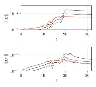
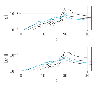
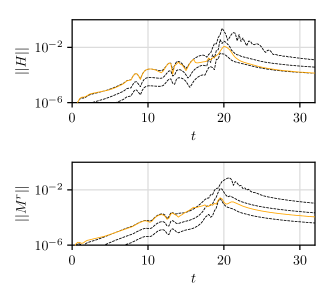
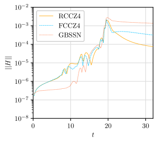
Figs. 4–7 show the performance of each formalism relative to one another. The simulations are run at a resolution of 4097 grid points on a grid which extends to $r=64$ (corresponding to the most refined unigrid run of Figs. 1–3). We choose the domain on which the norms are evaluated such that signals have not had sufficient time to propagate from the outer boundary (which is set assuming $X=1+a/r$ for some value $a$) into the domain of interest. It should be stressed that for all of the norms plotted in Figs. 4–7, the solutions are well resolved. The significant, and previously studied, improvements of the FCCZ4 method over GBSSN [7] in maintaining the Hamiltonian constraint and independent residuals is a real effect which is present even at high resolutions.

Figure 4: $l_{2}$ norm of the Hamiltonian constraint violation for the case of strong field initial data for each of GBSSN, FCCZ4 and RCCZ4. The difference between RCCZ4 and FCCZ4 is largely due to a more pronounced outgoing pulse of constraint violation (which leaves nearly flat space in its wake) while the large static constraint violation of GBSSN is concentrated at the origin and leaves behind a metric that does not appear to be a valid solution to the Einstein-scalar equations.

Figure 5: $l_{2}$ norm of the momentum constraint violation for the case of strong field initial data for each of GBSSN, FCCZ4 and RCCZ4. Not surprisingly, the performance of the three methods is largely equivalent as they are all designed to advect away the momentum constraint violation.

Figure 6: $l_{2}$ norm of $\bar{Z}_{r}=g_{a}(\accentset{\sim}{\Lambda}^{r}-\accentset{\sim}{\Delta}^{r})/2$ for the case of strong field initial data for each of GBSSN, FCCZ4 and RCCZ4. As in the case of the Hamiltonian constraint, the GBSSN errors are concentrated at the origin where the curvature takes on its largest values. This error remains essentially static save for the mitigating factor of dissipation. At this resolution, FCCZ4 preserves the constraint about 100 times better than GBSSN while RCCZ4 improves upon this by a further factor of $\sim 3$ or so at late times.

Figure 7: $l_{2}$ norm of the independent residual evaluator for $K_{b}$. At late times, as the solution should be approaching flat space, RCCZ4 has better performance than either FCCZ4 or GBSSN.

IV.2 Evolution of Black Hole Spacetimes

In order for RCCZ4 (or a to-be-developed formalism based upon similar principles) to be competitive with GBSSN or FCCZ4 in the domain of strong field numerical simulations (which frequently involve singularities), it first needs to be capable of stably evolving black holes. Here, we show that with minor modifications to the standard 1+log and Delta driver gauges, RCCZ4 in spherical symmetry is at least as capable as FCCZ4 for the evolution of black hole space times.

We start with standard time symmetric, black hole puncture initial data [12, 13] given by:

$$X =\left(1+\frac{M}{2r}\right)^{-2},$$ (75)

$$\alpha =\left(1+\frac{M}{2r}\right)^{-2},$$ (76)

$$\beta_{a} =K=A_{a}=A_{b}=0,$$ (77)

$$g_{a} =g_{b}=1.$$ (78)

The simulations are performed on large grids ($r=[0,128M]$ with $M=4$) which are further refined via fixed mesh refinement (FMR) . The sizes of the fixed refinement regions were determined by first evolving the initial data with adaptive mesh refinement. At the conclusion of this AMR run, each level of refinement had a maximum extent and that maximum extent then defined the limits of the corresponding level of refinement for the FMR calculations. In the simulations, the use of mesh refinement serves several purposes. First, it reduces the computational load for high resolution simulations. Second, it allows us to verify the compatibility of our implementation of the GBSSN, FCCZ4 and RCCZ4 formalisms with AMR. Third, by using fixed (as opposed to adaptive) mesh refinement, we eliminate complications caused by each formulation employing slightly different regridding procedures. This, in turn, facilitates the analysis of convergence properties. Table 1 shows the extent and refinement ratio of each grid used for the black hole simulations.

We note that the quantities $\bar{Z}_{i}$ and $\Theta$ are effectively error terms which serve to propagate violations of the momentum and Hamiltonian constraints and that they tend to grow in the vicinity of refinement boundaries. As such, we find that is is best to either evolve $\accentset{\sim}{\Lambda}^{i}$ (rather than $\bar{Z}_{i}$) or to omit $\Theta$ and $\bar{Z}_{i}$ from the truncation error calculation used to determine the placement of refined regions.

Level	$r_{\rm min}$	$r_{\rm max}$	$h^{0}_{r}$	$h^{1}_{r}$	$h^{2}_{r}$	$h^{3}_{r}$
1	0	512	8	4	2	1
2	0	512	4	2	1	$2^{-1}$
3	0	256	2	1	$2^{-1}$	$2^{-2}$
4	0	256	1	$2^{-1}$	$2^{-2}$	$2^{-3}$
5	0	128	$2^{-1}$	$2^{-2}$	$2^{-3}$	$2^{-4}$
6	0	64	$2^{-2}$	$2^{-3}$	$2^{-4}$	$2^{-5}$
7	0	32	$2^{-3}$	$2^{-4}$	$2^{-5}$	$2^{-6}$

Table 1: Parameters for the meshes in fixed mesh refinement convergence simulations. The fixed mesh refinement simulations use a total of 7 refinement levels as labeled in the first column. The extent of each mesh is displayed in columns 2 and 3 ($r_{\rm min}$ and $r_{\rm max}$). The grid spacings for the lowest resolution simulation are shown in the fourth column ($h^{0}_{r}$). Each of the final three columns ($h^{1}_{r}$, $h^{2}_{r}$ and $h^{3}_{r}$) give grid spacings for progressively higher resolution simulations. As an example, the $6^{\mathrm{th}}$ refinement level (Level 6) has a spatial extent of $r=[0,64]$. For the most resolved simulation ($h^{3}_{r}$), the grid spacing on that level is $2^{-5}$.

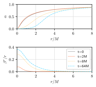
Figures 8–9 show the evolutions of $\alpha$, $\beta^{r}$ and $X$ as well as the coordinate location of the apparent horizon. determined by a zero of the quantity $\Xi$:

$$\Xi =\frac{rX\partial_{r}g_{b}}{2}-rg_{b}\partial_{r}X+g_{b}X-\frac{r\left(K+3A_{b}\right)}{3}.$$ (79)

As is well known [21, 15, 14, 22, 23, 1], puncture type initial data evolves towards a trumpet like spacetime and performs a form of automatic excision in the vicinity of the puncture. In this region, the evolved and constrained quantities do not converge.

Figure 8: Evolution of $\alpha$ and $\beta^{r}$ from $t=0$ to $t=64M=256$. The initial puncture type initial data quickly evolves towards trumpet type data with $\alpha$ going as $r$ as opposed to $r^{2}$ at the puncture.

Figure 9: Evolution of $X$ and $\Xi$ from $t=0$ to $t=64M=256$. The initial puncture type initial data quickly evolves towards trumpet type initial data with $X$ going as $r$ as opposed to $r^{2}$ at the puncture. As can be seen in the graph of $\Xi$, the coordinate location of the apparent horizon (where $\Xi=0$) increases slowly with coordinate time.

The convergence of the $l_{2}$ norms of the various constraints in the region external to the apparent horizon ($r=[r_{\mathrm{AH}},8M]$) and for each formalism are shown in Figs. 10–12. The dashed lines show simulations with $h_{r}=h^{0}_{r}$, $h_{r}=h^{1}_{r}$ and $h_{r}=h^{2}_{r}$ while the solid color denotes the most resolved $h_{r}=h^{3}_{r}$ simulation. Fig. 13 compiles the highest resolution runs of Figs. 10–12 and permits a direct comparison of the implementations. Independent residuals behave similarly and so have not been plotted.

Figure 10: $l_{2}$ norms of the Hamiltonian and momentum constraint violations for the GBSSN formulation. Each successive line denotes a factor of 2 grid refinement. The solid line denotes the most refined simulation.

Figure 11: $l_{2}$ norms of the Hamiltonian and momentum constraint violations for the FCCZ4 formulation. The errors in the momentum constraint appear to be dominated by artifacts that arise at the mesh refinement boundaries. Our GBSSN and RCCZ4 simulations used identical parameters and neither experienced the same sort of issues arising at the mesh refinement boundaries. Rather than attempting to find more optimal parameters which could resolve these issues at the cost of preventing direct comparison with GBSSN and RCCZ4, the simulation is left as-is and we note that it would almost certainly be possible to find better parameters for FCCZ4 which would mitigate these issues.

Figure 12: $l_{2}$ norms of the Hamiltonian and momentum constraint violations for the RCCZ4 formulation. Each successive line denotes a factor of 2 grid refinement. The solid line denotes the most refined simulation.

Figure 13: $l_{2}$ norms of the Hamiltonian constraint and momentum constraint violation for the $h_{r}=h^{3}_{r}$ run of each of the RCCZ4, FCCZ4 and GBSSN formulations. Here we can observe key differences in the constraint violating behaviours of each formulation. As the GBSSN simulation does not couple the Hamiltonian constraint to a propagating degree of freedom, errors within the horizon and at refinement boundaries are unable to propagate. Due to the fact that the black hole is not moving and the simulation quickly approaches a nearly stationary state, this lack of time dependence is advantageous. As shown in Section IV.1, the opposite is true when the simulation is highly dynamic. In those cases, both RCCZ4 and FCCZ4 provide orders of magnitude better constraint conservation.

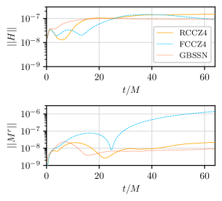
Examining Fig. 13, we see that for a stationary black hole, GBSSN is favoured over either FCCZ4 or RCCZ4. For a simulation where we are concerned with computing the constraint violation external to the apparent horizon, this makes intuitive sense: the formulation which does not propagate Hamiltonian constraint violations away from punctures or grid refinement boundaries should produce superior results when the fields are nearly stationary. However, as shown in [3], for more dynamical situations we should not expect superior performance from BSSN-type simulations even when constraint damping is employed.

As noted in Fig. 11, the errors in the momentum constraint (and $\bar{Z}_{r}$) for FCCZ4 appear to be dominated by the development of artifacts at the mesh refinement boundaries. Doubtless, these issues could be mitigated with proper attention. The relatively poor performance of FCCZ4 in comparison to GBSSN and RCCZ4 in these simulations should therefore not be seen as a shortcoming of the method, but as an issue arising from our demand that the methods be compared via runs with identical parameters. Taking this into account, we see that at early times (before the errors become dominated by issues arising from grid refinement boundaries), the performance of each method is roughly equivalent.

IV.3 Critical Collapse

Critical collapse represents the extreme strong field regime of general relativity and is therefore an excellent test case to determine the capabilities of a numerical formulation. Here we compare the RCCZ4, FCCZ4 and GBSSN formalisms, without constraint damping, in a test that studies each formalism’s capacity to resolve the threshold of black hole formation using gauges which are natural extensions of the 1+log slicing, (71–73), with zero shift. For additional information concerning critical collapse, see [24] for the original study concerning the massless scalar field in spherical symmetry and [25, 26] for more general reviews.

For each of GBSSN, FCCZ4 and RCCZ4, we perform AMR simulations of massless scalar field collapse with a relative, per-step truncation error tolerance of $10^{-4}$. We tune the amplitude of our initial data to the threshold of black hole formation with a relative tolerance of $\sim 10^{-12}$.

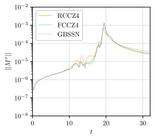
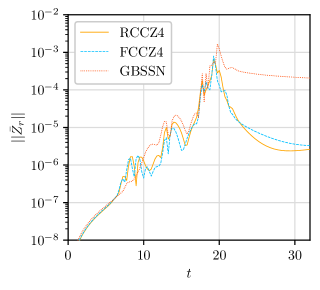
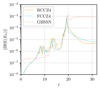
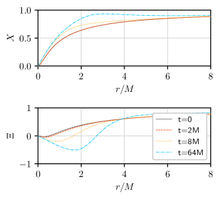
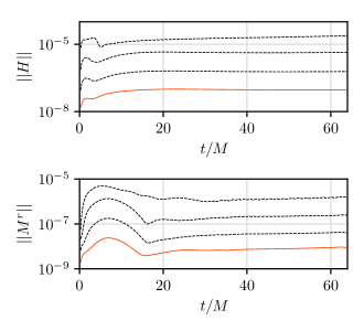
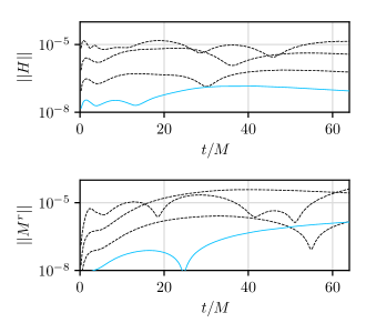
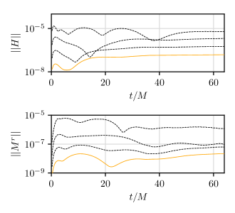
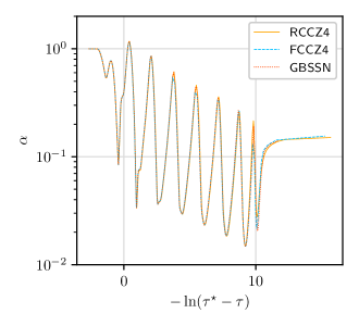
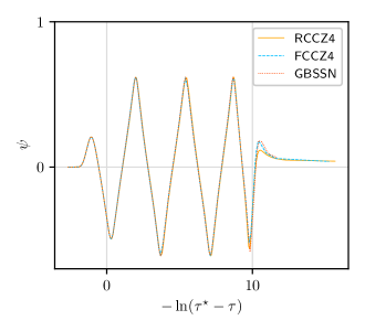
Figures 14–15 plot the central value of the lapse and the scalar field, respectively, against proper time at the approximate accumulation point (the spacetime point at which a naked singularity would form in the limit of infinite tuning) for the subcritical simulation closest to criticality in each formalism. Figures. 16–18 plot the magnitudes of constraint violations from these calculations. For these simulations we expect all dimensionful quantities to grow exponentially in $-\ln{(\tau^{\star}-\tau)}$ due to the discretely self-similar nature of the critical solution. To facilitate analysis of the overall growth rate of constraint violations, we plot the cumulative maximum, $\mathrm{cummax}(f(t),t)$, of each quantity. This function returns the largest magnitude encountered on the domain of the simulation up until that point in time (e.g. $\mathrm{cummax}(R,t_{0})$ would return the largest value of $R$ encountered during the simulation for $t=[0,t_{0}]$).

Figure 14: Lapse, $\alpha$, at the accumulation point as a function of $-\ln(\tau^{\star}-\tau)$ with $\tau^{\star}$ an approximate accumulation time which is different for each set of simulations. Each of GBSSN, FCCZ4 and RCCZ4 are well suited to performing the critical evolutions. The observed discrepancies in $\alpha$ are primarily due to our output of data with insufficient frequency to resolve the peaks adequately. As expected, we are able to resolve approximately 3 echos at a relative search tolerance of $10^{-12}$.

Figure 15: Scalar field, $\psi$, at the accumulation point as a function of $-\ln(\tau^{\star}-\tau)$. The discrete self similarity (DSS) is evident. Tuning the amplitude of our initial data to the threshold of black hole formation with a relative tolerance of $\sim 10^{-12}$ allows us to resolve approximately three echos.

Figure 16: Cumulative maximal values of $R$, $\bar{Z}_{r}$, the Hamiltonian constraint and momentum constraint violations for critical collapse of the scalar field in the GBSSN formulation. For clarity, we have not shown the behaviour of the Hamiltonian constraint post-dispersal, where it is dominated by a large non propagating remnant similar to that seen in Fig. 1.

Figure 17: Cumulative maximal values of $R$, $\bar{Z}_{r}$, the Hamiltonian constraint and momentum constraint violations for critical collapse of the scalar field in the FCCZ4 formulation. For subcritical simulations close to criticality, the post dispersal constraint violating remnant is much smaller than that of GBSSN but is still too large to continue the simulation for long periods of time.

Figure 18: Cumulative maximal values of $R$, $\bar{Z}_{r}$, the Hamiltonian constraint and momentum constraint violations for critical collapse of the scalar field in the RCCZ4 formulation. For subcritical simulations close to criticality, the post dispersal constraint violating remnant is much smaller than that of GBSSN but is still too large to continue the simulation for long periods of time. Close to criticality, the constraint violations grow noticeably faster than either GBSSN or FCCZ4 (while still providing adequate resolution to investigate criticality).

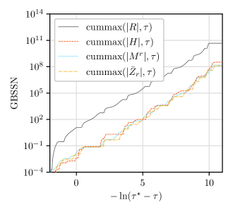
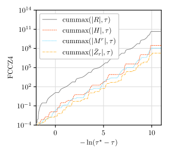
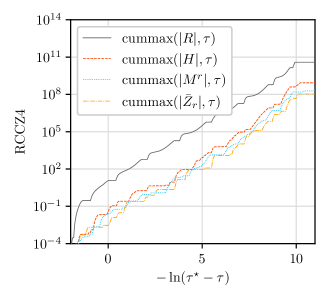
As seen in Figs. 16–18, when evolved using identical error tolerances and parameters, we find that GBSSN does the best at maintaining a constant level of relative constraint violation throughout the simulation. We find that with a per-step error tolerance of $10^{-4}$, GBSSN maintains a constant error ratio of about $10^{-3}$ relative to the magnitude of the Ricci scalar. For FCCZ4, this is reduced to $10^{-2}$ while RCCZ4 performs similarly to FCCZ4 for the first echo or so and then gradually accumulates more error, performing worse than either GBSSN or FCCZ4 at late times.

At this point, the cause of this dip in performance for RCCZ4 is unclear to us. However, it is entirely possible that it is due to a suboptimal regridding strategy. Alternatively, it could very well be that the variant of the 1+log slicing condition used, Eqn. (73), is not ideal for controlling the Hamiltonian constraint. We tried several variations of the form $\partial_{t}\alpha=-2\alpha(K-2f(\alpha)\accentset{\sim}{\Theta})$, which, for the most part, resulted in similar performance and stability properties.

The superior performance of GBSSN in the approach to criticality contrasts with its poor performance post dispersal. As in Sec. IV.1, after a simulation achieves its closest approach to criticality, the scalar field disperses to infinity and would ideally leave flat space in its wake. Both FCCZ4 and RCCZ4 perform better than GBSSN in this regime although this is not evident when plotting cumulative maxima as in Figs. 16–18.

V Hyperbolicity of RCCZ4

We now turn to an analysis of the hyperbolicity of RCCZ4. We demonstrate that, relative to GBSSN, RCCZ4 has one fewer zero-velocity modes, which roughly corresponds to the fact that in Z4 derived formulations the equivalent of the Hamiltonian constraint is dynamical [3, 7, 27]. As outlined in [28, 29, 30], and in the context of numerical relativity, these zero-velocity modes often correspond to constraint violations and are thought to contribute to instabilities. Consequently, formulations that minimize these modes are generally favoured.

Here we derive the conditions under which RCCZ4 is hyperbolic, performing a pseudodifferential reduction [31, 5] following the procedure of Cao and Wu [28] who have previously applied the method to a study of the hyperbolicity of BSSN in $f(R)$ gravity. We consider the RCCZ4 equations of motion (32)–(38) in the vacuum and choose a generalization of the Bona-Masso family of lapses [32, 12] together with generalized Lambda drivers for the shift. Specifically, defining

$$\partial_{0} =\partial_{t}-\beta^{i}\partial_{i}$$ (80)

the equation for the lapse is

$$\partial_{0}\alpha =-\alpha^{2}h\left(\alpha,\chi\right)\left(\frac{}{}K-K_{0}-\frac{m\left(\alpha,\chi\right)}{\alpha}\accentset{\sim}{\Theta}\right).$$ (81)

Our generalized Lambda driver takes the form

$$\partial_{0}\beta^{i} =\alpha^{2}G\left(\alpha,\chi\right)B^{i},$$ (82)

where the auxiliary vector $B^{i}$ satisfies

$$\partial_{0}B^{i} =e^{-4\chi}H\left(\alpha,\chi\right)\partial_{0}\accentset{\sim}{\Lambda}^{i}-\eta\left(B^{i},\alpha\right),$$ (83)

and $G$ and $H$ are some specified functions.

We wish to determine the conditions under which the RCCZ4 system is strongly hyperbolic. This essentially amounts to verifying that the system admits a well defined Cauchy problem; i.e. that there exist no high frequency modes with growth rates which cannot be bounded by some exponential function of time [5]. We can thus study strong hyperbolicity by linearizing the equations about some generic solution and examining the resulting perturbed system in the high frequency regime where it takes the form

$$\partial_{0}u=\mathbf{M}^{i}\partial_{i}u+\mathbf{S}u.$$ (84)

Here, $u$ is a vector of $n$ perturbation fields, $\mathbf{M}^{i}$ are $n$-by-$n$ characteristic matrices and $\mathbf{S}u$ is a source vector that may depend on the fundamental variables $u$ but not on their derivatives. Fourier transforming the perturbation $u$ via

$$\hat{u}\left(\omega\right)=\int{e^{i(\omega_{k}x^{k})}u\left(x\right)\mathrm{d}^{3}x},$$ (85)

we can write (84) as

$$\partial_{0}\hat{u}=i\omega_{i}\mathbf{M}^{i}\hat{u}+\mathbf{S}\hat{u}.$$ (86)

From this, we define the principal symbol of the system as $\mathbf{P}_{1}=i\left|\omega\right|\mathbf{P}=i\omega_{i}\mathbf{M}^{i}$. The hyperbolicity of the system can then be discerned from the properties of $\mathbf{P}$:

• If $\mathbf{P}$ has imaginary eigenvalues, the system is not hyperbolic and cannot be formulated as a well-posed Cauchy problem.

• If $\mathbf{P}$ has only real eigenvalues but does not possess a complete set of eigenvectors, the system is weakly hyperbolic and may have issues with ill-posedness.

• If $\mathbf{P}$ has both real eigenvalues and a complete set of eigenvectors, the system is strongly hyperbolic and the Cauchy problem is well-posed.

Returning to the specific case of the RCCZ4 formulation in vacuum, we linearize (32)–(38) about some generic solution and consider perturbations in the high frequency regime. In such a regime, the length scale associated with the unperturbed solution will be large relative to the perturbations and we may safely freeze the coefficients in the perturbed equations. Upon decomposing the resulting linear constant coefficient into Fourier modes, we obtain:

$$\partial_{0}\hat{\chi} =-\frac{1}{6}\alpha\hat{K}+\frac{1}{6}\left(i\omega_{k}\right)\hat{\beta}^{k},$$ (87)

$$\partial_{0}\hat{K} =\alpha\hat{R}+\omega_{l}\omega_{m}\gamma^{lm}\hat{\alpha}+2\alpha\gamma^{lm}\left(i\omega_{l}\hat{Z}_{m}\right),$$ (88)

$$\partial_{0}\hat{\accentset{\sim}{\Theta}} =\frac{1}{2}\alpha^{2}\left(\hat{R}+2\left(i\omega_{i}\right)\hat{Z}_{j}\gamma^{ij}\right),$$ (89)

$$\partial_{0}\hat{\accentset{\sim}{\gamma}}_{ij} =-2\alpha\hat{\accentset{\sim}{A}}_{ij}-\frac{2}{3}\accentset{\hphantom{i}\sim}{\gamma}_{ij}\left(i\omega_{m}\right)\hat{\beta}^{m}$$ (90)

$$\hphantom{=}+\accentset{\hphantom{i}\sim}{\gamma}_{im}\left(i\omega_{j}\right)\hat{\beta}^{m}+\accentset{\hphantom{i}\sim}{\gamma}_{mj}\left(i\omega_{i}\right)\hat{\beta}^{m},$$

$$\partial_{0}\hat{\accentset{\sim}{A}}_{ij} =e^{-4\chi}\left[\omega_{i}\omega_{j}\gamma^{ij}\hat{\alpha}+\alpha\hat{R}_{ij}\right.$$ (91)

$$\mathopen{}\left.\vphantom{\frac{}{}}\hphantom{=}+2\alpha\left(i\omega_{(i}\hat{Z}_{j)}\right)\right]^{\mathrm{TF}},$$

$$\partial_{0}\hat{\accentset{\sim}{\Lambda}}^{i} =\accentset{\hphantom{i}\sim}{\gamma}^{mn}\left(-\omega_{m}\omega_{n}\right)\hat{\beta}^{i}+\frac{1}{3}\accentset{\hphantom{i}\sim}{\gamma}^{ik}\left(-\omega_{k}\omega_{n}\right)\hat{\beta}^{n}$$ (92)

$$\hphantom{=}-\frac{4}{3}\alpha\accentset{\hphantom{i}\sim}{\gamma}^{ij}\left(i\omega_{j}\right)\hat{K}+2\accentset{\hphantom{i}\sim}{\gamma}^{ik}\left(i\omega_{k}\right)\hat{\accentset{\sim}{\Theta}},$$

$$\partial_{0}\hat{Z}_{i} =\alpha\left[\left(i\omega_{j}\right)\hat{\accentset{\sim}{A}}_{ki}\accentset{\hphantom{i}\sim}{\gamma}^{jk}-\frac{2}{3}\left(i\omega_{i}\right)\hat{K}\right]+\left(i\omega_{j}\right)\hat{\accentset{\sim}{\Theta}},$$ (93)

$$\partial_{0}\hat{\alpha} =-\alpha^{2}h\hat{K}+\alpha{h}{m}\hat{\accentset{\sim}{\Theta}},$$ (94)

$$\partial_{0}\hat{\beta}^{i} =\alpha^{2}G\hat{B}^{i},$$ (95)

$$\partial_{0}\hat{B}^{i} =2H\gamma^{im}\partial_{0}\hat{Z}_{m}+H\left(i\omega^{n}\right)\accentset{\hphantom{i}\sim}{\gamma}^{mi}\partial_{0}\hat{\accentset{\sim}{\gamma}}_{mn}.$$ (96)

Here, since we are interested in the high frequency regime, we have kept only the leading order derivative terms. In these equations, $\hat{R}_{ij}$ may either be considered as a function of $\scalebox{1.0}{$\accentset{\sim}{\Lambda}$}\vphantom{}^{i}$ (as would be the case for GBSSN):

$$\hat{R}_{ij} =\frac{1}{2}\accentset{\hphantom{i}\sim}{\gamma}^{lm}\left(\omega_{l}\omega_{m}\right)\hat{\accentset{\sim}{\gamma}}_{ij}+\frac{1}{2}\accentset{\hphantom{i}\sim}{\gamma}_{mi}\left(i\omega_{j}\right)\hat{\accentset{\sim}{\Lambda}}^{m}$$ (97)

$$\hphantom{=}+\frac{1}{2}\accentset{\hphantom{i}\sim}{\gamma}_{mj}\left(i\omega_{i}\right)\hat{\accentset{\sim}{\Lambda}}^{m}+2\left(\omega_{i}\omega_{j}\right)\hat{\chi}$$

$$\hphantom{=}+2\gamma_{ij}\gamma^{lm}\left(\omega_{l}\omega_{m}\right)\hat{\chi},$$

or as a function of $\scalebox{1.0}{$\accentset{\sim}{\Delta}$}\vphantom{}^{i}$ (as derived in Sec. II):

$$\hat{R}_{ij} =\frac{1}{2}\accentset{\hphantom{i}\sim}{\gamma}^{lm}\left(\omega_{l}\omega_{m}\right)\hat{\accentset{\sim}{\gamma}}_{ij}+\frac{1}{2}\accentset{\hphantom{i}\sim}{\gamma}_{mi}\left(i\omega_{j}\right)\hat{\accentset{\sim}{\Delta}}^{m}$$ (98)

$$\hphantom{=}+\frac{1}{2}\accentset{\hphantom{i}\sim}{\gamma}_{mj}\left(i\omega_{i}\right)\hat{\accentset{\sim}{\Delta}}^{m}+2\left(\omega_{i}\omega_{j}\right)\hat{\chi}$$

$$\hphantom{=}+2\gamma_{ij}\gamma^{lm}\left(\omega_{l}\omega_{m}\right)\hat{\chi}.$$

In what follows, $\epsilon=1$ corresponds to the use of $\scalebox{1.0}{$\accentset{\sim}{\Delta}$}\vphantom{}^{i}$ while $\epsilon=2$ corresponds to the definition in terms of $\scalebox{1.0}{$\accentset{\sim}{\Lambda}$}\vphantom{}^{i}$. Roughly following [28], we introduce the variables:

$$\omega_{i} =\left|\omega\right|\accentset{\sim}{\omega}_{i},$$ (99)

$$\left|\omega\right|^{2} =\gamma^{ij}\omega_{i}\omega_{j},$$ (100)

$$\hat{\alpha} =\frac{-i\alpha}{\left|\omega\right|}\hat{a},$$ (101)

$$\hat{\chi} =\frac{-i}{\left|\omega\right|}\hat{X},$$ (102)

$$\hat{\accentset{\sim}{\Theta}} =\alpha\hat{\Omega},$$ (103)

$$\hat{\accentset{\sim}{\Lambda}}^{i} =\accentset{\hphantom{i}\sim}{\gamma}^{ij}\hat{\accentset{\sim}{\Lambda}}_{j},$$ (104)

$$\hat{\beta}^{i} =\frac{-i\alpha}{\left|\omega\right|}\gamma^{ij}\hat{b}_{j},$$ (105)

$$\hat{B}^{i} =\gamma^{ij}\hat{B}_{j},$$ (106)

$$\hat{\accentset{\sim}{\gamma}}_{ij} =\frac{-ie^{-4\chi}}{\left|\omega\right|}\hat{l}_{ij},$$ (107)

$$\hat{\accentset{\sim}{A}}_{ij} =e^{-4\chi}\hat{L}_{ij},$$ (108)

which permits us to write (87)–(96) as a first order pseudodifferential system of the form

$$\partial_{0}\hat{u} =i\left|\omega\right|\alpha\mathbf{P}\hat{u},$$ (109)

where

$$\hat{u} =\begin{bmatrix}\hat{a}&\hat{\chi}&\hat{\Omega}&\hat{K}&\hat{b}_{i}&\hat{B}_{i}&\hat{\accentset{\sim}{\Lambda}}_{i}&\hat{l}_{ij}&\hat{L}_{ij}\end{bmatrix}^{\mathrm{T}}.$$ (110)

Provided that $\mathbf{P}$ is diagonalizable with purely real eigenvalues, the system will be strongly hyperbolic [5, 28, 30]. Then, following the methodology of Nagy et al. [5, 28], we decompose the eigenvalue equation

$$\mathbf{P}\hat{u}=\lambda\hat{u},$$ (111)

by projecting $\hat{u}$ into longitudinal and transverse components with respect to $\accentset{\sim}{\omega}_{i}$ via application of the projection operator

$$q_{ij} =\gamma_{ij}-\accentset{\sim}{\omega}_{i}\accentset{\sim}{\omega}_{j}.$$ (112)

Explicitly, we split all rank-1 and 2 covariant tensors into their components in and orthogonal to $q_{ij}$. In such a decomposition, symmetric rank-2 tensors on the 3D hypersurface with metric $\gamma_{ij}$ may be represented as:

$$\hat{X}_{ij} =\accentset{\sim}{\omega}_{i}\accentset{\sim}{\omega}_{j}\hat{X}+\frac{1}{2}q_{ij}\hat{X}^{{}^{\prime}}+2\accentset{\sim}{\omega}_{(i}\hat{X}^{{}^{\prime}}_{j)}+\hat{X}^{{}^{\prime}}_{\langle ij\rangle},$$ (113)

with

$$\hat{X} =\accentset{\sim}{\omega}^{i}\accentset{\sim}{\omega}^{j}\hat{X}_{ij},$$ (114)

$$\hat{X}^{{}^{\prime}} =q^{ij}\hat{X}_{ij},$$ (115)

$$\hat{X}^{{}^{\prime}}_{i} ={q_{i}}^{j}\accentset{\sim}{\omega}^{k}\hat{X}_{jk},$$ (116)

$$\hat{X}^{{}^{\prime}}_{\langle ij\rangle} ={q_{i}}^{l}{q_{j}}^{m}\left(\hat{X}_{lm}-\frac{1}{2}\hat{X}^{{}^{\prime}}q_{lm}\right),$$ (117)

and where angle brackets denote a tensorial quantity which is trace free with respect to $q_{ij}$. Similarly, covectors may be split according to

$$\hat{Y}_{i} =\omega_{i}\hat{Y}+\hat{Y}^{{}^{\prime}}_{i},$$ (118)

with

$$\hat{Y} =\accentset{\sim}{\omega}^{i}\hat{Y}_{i},$$ (119)

$$\hat{Y}^{{}^{\prime}}_{i} ={q_{i}}^{j}\hat{Y}_{j}.$$ (120)

Upon application of these tensor and vector decompositions to (109), we find that $\mathbf{P}$ can be written in block diagonal form:

$$\mathbf{P} =\begin{bmatrix}\mathbf{P}^{\mathrm{S}}&0&0\\ 0&\mathbf{P}^{\mathrm{V}}&0\\ 0&0&\mathbf{P}^{\mathrm{T}}\end{bmatrix},$$ (121)

with $\mathbf{P}^{\mathrm{S}}$ , $\mathbf{P}^{\mathrm{V}}$ and $\mathbf{P}^{\mathrm{T}}$ denoting scalar, vector and tensor components. Following a lengthy calculation, we find the following results for (1) the scalar components:

$$\partial_{0}\hat{a} =i\left|\omega\right|\alpha\left[-h\hat{K}+{h}{m}\hat{\Omega}\right],$$ (122)

$$\partial_{0}\hat{b} =i\left|\omega\right|\alpha\left[G\hat{B}\right],$$ (123)

$$\partial_{0}\hat{B} =i\left|\omega\right|\alpha\left[\frac{4H}{3}\hat{b}-\frac{4H}{3}\hat{K}+2H\hat{\Omega}\right],$$ (124)

$$\partial_{0}\hat{X} =i\left|\omega\right|\alpha\left[\frac{1}{6}\hat{b}-\frac{1}{6}\hat{K}\right],$$ (125)

$$\partial_{0}\hat{l} =i\left|\omega\right|\alpha\left[\frac{4}{3}\hat{b}-2\hat{L}\right],$$ (126)

$$\partial_{0}\hat{l}^{{}^{\prime}} =i\left|\omega\right|\alpha\left[-\frac{4}{3}\hat{b}+2\hat{L}\right],$$ (127)

$$\partial_{0}\hat{K} =i\left|\omega\right|\alpha\left[-\hat{a}-8\hat{X}+\frac{1}{2}\hat{l}-\frac{1}{2}\hat{l}^{{}^{\prime}}+2\epsilon\hat{Z}\right],$$ (128)

$$\partial_{0}\hat{\Omega} =i\left|\omega\right|\alpha\left[-4\hat{X}+\frac{1}{4}\hat{l}-\frac{1}{4}\hat{l}^{{}^{\prime}}+\epsilon\hat{Z}\right],$$ (129)

$$\partial_{0}\hat{L} =i\left|\omega\right|\alpha\left[-\frac{2}{3}\hat{a}-\frac{4}{3}\hat{X}+\frac{1}{3}\hat{l}+\frac{1}{6}\hat{l}^{{}^{\prime}}+\frac{4\epsilon}{3}\hat{Z}\right],$$ (130)

$$\partial_{0}\hat{Z} =i\left|\omega\right|\alpha\left[\hat{L}-\frac{2}{3}\hat{K}+\hat{\Omega}\right],$$ (131)

(2) the vector components:

$$\partial_{0}\hat{b}^{{}^{\prime}}_{i} =i\left|\omega\right|\alpha\left[G\hat{B}^{{}^{\prime}}_{i}\right],$$ (132)

$$\partial_{0}\hat{B}^{{}^{\prime}}_{i} =i\left|\omega\right|\alpha\left[H\hat{b}^{{}^{\prime}}_{i}\right],$$ (133)

$$\partial_{0}\hat{l}^{{}^{\prime}}_{i} =i\left|\omega\right|\alpha\left[\hat{b}^{{}^{\prime}}_{i}-2\hat{L}^{{}^{\prime}}_{i}\right],$$ (134)

$$\partial_{0}\hat{L}^{{}^{\prime}}_{i} =i\left|\omega\right|\alpha\left[\epsilon\hat{Z}^{{}^{\prime}}_{i}\right],$$ (135)

$$\partial_{0}\hat{Z}^{{}^{\prime}}_{i} =i\left|\omega\right|\alpha\left[\hat{L}^{{}^{\prime}}_{i}\right],$$ (136)

and (3) tensor components:

$$\partial_{0}\hat{l}^{{}^{\prime}}_{\langle ij\rangle} =i\left|\omega\right|\alpha\left[-2\hat{L}^{{}^{\prime}}_{\langle ij\rangle}\right],$$ (137)

$$\partial_{0}\hat{L}^{{}^{\prime}}_{\langle ij\rangle} =i\left|\omega\right|\alpha\left[-\frac{1}{2}\hat{l}^{{}^{\prime}}_{\langle ij\rangle}\right].$$ (138)

Note that since $\hat{A}_{ij}$ is trace-free we have $\hat{L}^{{}^{\prime}}=-\hat{L}$, which is why no evolution equation for $\hat{L}^{{}^{\prime}}$ appears. Expressing these systems of equations as matrix equations of the form (111) and (121), the eigenvalues of $\mathbf{P}^{\mathrm{S}}$ are:

$$\lambda =0,\,0,\,\pm 1,\,\pm\sqrt{\epsilon},\,\pm\sqrt{h},\,\pm\sqrt{\frac{4}{3}GH}.$$ (139)

Comparing with the results of [27, 28] (which consider various BSSN-type systems), we observe that RCCZ4 has one fewer zero velocity eigenvalue than GBSSN. It is this eigenvalue which corresponds to the Hamiltonian constraint advection and it is largely responsible for the superior performance of FCCZ4 relative to GBSSN [7, 27, 3]. Treating $\accentset{\sim}{R}_{ij}$ as a function of $\accentset{\sim}{\Lambda}^{i}$ versus $\accentset{\sim}{\Delta}^{i}$ ($\epsilon=2$ versus $\epsilon=1$) has the effect of increasing the speed of propagation of several modes, but otherwise has no effect on hyperbolicity. In fact, we see that RCCZ4 appears to be well defined for a fairly wide range of $\epsilon$ which roughly corresponds to modified equations of motion in which the Ricci tensor is supplemented by additional terms of the form $\accentset{\sim}{D}_{(i}\bar{Z}_{j)}$.

In the case of the vector components, the eigenvalues of the matrix $\mathbf{P}^{\mathrm{V}}$ each have multiplicity 2 (rather than 3) due to the projection constraints of the form $\accentset{\sim}{\omega}^{i}\hat{X}_{i}=0$. The eigenvalues are:

$$\lambda =0,\,\pm\sqrt{\epsilon},\,\pm\sqrt{GH}.$$ (140)

Finally, for the tensor components, the eigenvalues of $\mathbf{P}^{\mathrm{T}}$ have multiplicity 2 (rather than 6) due to the three projection constraints of the form $\accentset{\sim}{\omega}^{i}\hat{X}^{{}^{\prime}}_{ij}=0$ and the trace-free condition $\hat{X}^{{}^{\prime}}_{\langle ij\rangle}\gamma^{ij}=0$. The eigenvalues are the same as we would find for BSSN and ADM [28, 5, 27]:

$$\lambda =\pm 1.$$ (141)

In order to guarantee weak hyperbolicity, all of these eigenvalues must be real, so we must have

$$GH>0,\;h>0,\;\epsilon>0.$$ (142)

Strong hyperbolicity additionally requires that each of $\mathbf{P}^{S}$, $\mathbf{P}^{V}$ and $\mathbf{P}^{T}$ are diagonalizable. For this to be the case, all of the following conditions must hold:

$$h\neq\epsilon,\;HG\neq\frac{3}{4},\;HG\neq\frac{3}{4}h,\;HG\neq\frac{3}{4}\epsilon,$$ (143)

so that $\mathbf{P}$ has a complete set of eigenvectors. Here, $\epsilon\notin\{1,2\}$ would occur if we were to substitute some other combination of $\accentset{\sim}{\Delta}^{i}$ and $\accentset{\hphantom{i}\sim}{\gamma}^{ij}\bar{Z}_{j}$ in the definition of $\accentset{\sim}{R}_{ij}$. Note that as $h$, $G$ and $H$ are generically functions of $\alpha$ and $\chi$, we cannot guarantee that our equations of motion will be everywhere strongly hyperbolic. However, if we perform the same sort of pseudodifferential decomposition for FCCZ4 (using a slightly modified gauge), we find that RCCZ4 and FCCZ4 share the same principal part and we thus conclude that the two methods have identical stability characteristics in the high frequency limit.

VI Summary and Conclusions

In this paper, we have introduced our novel RCCZ4 formulation of numerical relativity. We have demonstrated that it is possible to achieve roughly equivalent performance to GBSSN and FCCZ4 through a modification of Z4 wherein constraint violations are coupled to a reference metric completely independent of the physical metric. We have shown that this approach works in the presence of black holes and holds up robustly in a variety of 1D simulations including the critical collapse of a scalar field. In addition to stably evolving spherically symmetric simulations in the strong field, we have demonstrated that our formulation is strongly hyperbolic through the use of a pseudodifferential first order reduction.

Our formulation of RCCZ4 chose the simplest possible reference metric, but we can easily imagine formulations in which the components of $\accentset{\circ}{g}_{\mu\nu}$ are chosen or evolved in such a way so as to provide additional beneficial properties aside from the vanishing of the Ricci tensor. We suspect that it will be in modifications to the choice of $\accentset{\circ}{g}_{\mu\nu}$ in which the full utility of RCCZ4-like formulations is realized.

The core idea behind RCCZ4—coupling the constraint equations to a metric different from the physical metric—could potentially be used to derive methods with greater stability and superior error characteristics than either GBSSN or FCCZ4. In our opinion, the main takeaway should not be that RCCZ4, as it stands, is a complete formulation with performance approaching or exceeding FCCZ4 and GBSSN. Rather, the main lesson should be that the Z4 formulation of general relativity can be modified such that the constraints are coupled to a metric other then the physical one, and that such a modification may be useful in tailoring the properties of the system as they pertain to constraint advection and damping.

Appendix A 3+1 Form of RZ4

The RZ4 equations in canonical and trace-reversed form with damping are given by (10) and (11). As we have been predominantly interested in investigating scale invariant problems, we set the damping parameters $\kappa_{1}$ and $\kappa_{2}$ to zero, yielding the simpler set of equations:

$$R_{\mu\nu}-\frac{1}{2}g_{\mu\nu}R+2\accentset{\circ}{\nabla}_{(\mu}Z_{\nu)}-g_{\mu\nu}\accentset{\circ}{\nabla}_{(\alpha}Z_{\beta)}g^{\alpha\beta}$$ (144)

$$\hphantom{=}-8\pi T_{\mu\nu}=0,$$

$$R_{\mu\nu}+2\accentset{\circ}{\nabla}_{(\mu}Z_{\nu)}-8\pi\left(T_{\mu\nu}-\frac{1}{2}g_{\mu\nu}T\right)=0,$$ (145)

$$R+2\accentset{\circ}{\nabla}_{(\mu}Z_{\nu)}g^{\mu\nu}+8\pi T=0.$$ (146)

Here, (144) is RZ4 written in canonical form, (145) is written in trace-reversed form and (146) is the trace of (145) taken with respect to the physical metric $g^{\mu\nu}$.

To derive the ADM equivalent of the RZ4 equations we roughly follow the ADM derivations of [12, 13] and take projections of (144)–(146) onto and orthogonal to the spatial hypersurfaces which foliate four dimensional spacetime in a standard 3+1 decomposition. In what follows, we consider only the simplest case where $\accentset{\circ}{g}_{\mu\nu}$ is a time-invariant, curvature-free, Lorentzian metric with $\accentset{\circ}{g}_{tt}=-1,\accentset{\circ}{g}_{tj}=0$.

A.1 Spatial projection

We begin by finding the evolution equation for the extrinsic curvature by projecting both indices of (145) onto $\Sigma$. The terms present in the Einstein equations follow the ordinary ADM derivation so we concentrate on the terms containing $Z^{\mu}$:

$$\gamma^{\mu}\vphantom{}_{\lambda}\gamma^{\nu}\vphantom{}_{\sigma}\accentset{\circ}{\nabla}_{\mu}Z_{\nu} =\gamma^{\mu}\vphantom{}_{\lambda}\gamma^{\nu}\vphantom{}_{\sigma}\left(\vphantom{\frac{}{}}\partial_{\mu}{\bar{Z}}_{\nu}+\Theta\partial_{\mu}n_{\nu}\right.$$ (147)

$$\mathopen{}\left.\hphantom{=}-\accentset{\circ}{\Gamma}^{\rho}\vphantom{}_{\mu\nu}\left({\bar{Z}}_{\rho}+n_{\rho}\Theta\right)\right).$$

We now note that, since $n_{i}=0$, when restricting to spatial indices we have:

$$\gamma^{\mu}\vphantom{}_{l}\gamma^{\nu}\vphantom{}_{m}\partial_{\mu}n_{\nu} =\left({\delta^{\mu}}_{l}+n^{\mu}n_{l}\right)\left({\delta^{\nu}}_{m}+n^{\nu}n_{m}\right)\partial_{\mu}n_{\nu},$$ (148)

$$=\left({\delta^{\mu}}_{l}{\delta^{\nu}}_{m}+{\delta^{\mu}}_{l}n^{\nu}n_{m}+{\delta^{\nu}}_{m}n^{\mu}n_{l}\right.$$

$$\mathopen{}\left.\hphantom{=}+n^{\mu}n_{l}n^{\nu}n_{m}\right)\partial_{\mu}n_{\nu},$$

$$=\left(\partial_{l}n_{m}+n^{\nu}n_{m}\partial_{l}n_{\nu}+n^{\mu}n_{l}\partial_{\mu}n_{m}\right.$$

$$\mathopen{}\left.\hphantom{=}+n^{\mu}n_{l}n^{\nu}n_{m}\partial_{\mu}n_{\nu}\right),$$

$$=0,$$

and therefore

$$2\gamma^{\mu}\vphantom{}_{i}\gamma^{\nu}\vphantom{}_{j}\accentset{\circ}{\nabla}_{(\mu}Z_{\nu)} =2\gamma^{\mu}\vphantom{}_{i}\gamma^{\nu}\vphantom{}_{j}\left(\partial_{(\mu}{\bar{Z}}_{\nu)}+\Theta\partial_{(\mu}n_{\nu)}\right.$$ (149)

$$\mathopen{}\left.\hphantom{=}-\accentset{\circ}{\Gamma}^{\rho}\vphantom{}_{\mu\nu}\left({\bar{Z}}_{\rho}+n_{\rho}\Theta\right)\right),$$

$$=2\gamma^{\mu}\vphantom{}_{i}\gamma^{\nu}\vphantom{}_{j}\left(\partial_{(\mu}{\bar{Z}}_{\nu)}-\accentset{\circ}{\Gamma}^{\rho}\vphantom{}_{\mu\nu}\left({\bar{Z}}_{\rho}+n_{\rho}\Theta\right)\vphantom{\frac{}{}}\right).$$

Assuming $\accentset{\circ}{g}_{\mu\nu}=\delta_{tt}+\accentset{\hphantom{i}\circ}{\gamma}_{ij}$ with $\accentset{\circ}{R}_{ij}={\accentset{\circ}{\Gamma}^{t}}_{ij}=0$ (e.g. we take the simplest possible flat background 3-metric), this simplifies further to,

$$2\gamma^{\mu}\vphantom{}_{i}\gamma^{\nu}\vphantom{}_{j}\accentset{\circ}{\nabla}_{(\mu}Z_{\nu)}= 2\gamma^{\mu}\vphantom{}_{i}\gamma^{\nu}\vphantom{}_{j}\left(\partial_{(\mu}{\bar{Z}}_{\nu)}-\accentset{\circ}{\Gamma}^{k}\vphantom{}_{\mu\nu}{\bar{Z}}_{k}\right),$$ (150)

$$= 2\left(\delta^{\mu}\vphantom{}_{i}\delta^{\nu}\vphantom{}_{j}+\delta^{\mu}\vphantom{}_{i}n^{\nu}n_{j}+\delta^{\nu}\vphantom{}_{j}n^{\nu}n_{i}\right.$$

$$\mathopen{}\left.+n^{\mu}n_{i}n^{\nu}n_{j}\right)\left(\partial_{(\mu}{\bar{Z}}_{\nu)}-\accentset{\circ}{\Gamma}^{k}\vphantom{}_{\mu\nu}{\bar{Z}}_{k}\right),$$

$$= 2\partial_{(i}{\bar{Z}}_{j)}-2\accentset{\circ}{\Gamma}^{k}\vphantom{}_{ij}{\bar{Z}}_{k},$$

$$= 2\accentset{\circ}{D}_{(i}{\bar{Z}}_{j)}\,.$$

Here, we have made use of the fact that, with the connection given above, the Christoffel symbols for the spatial component of the background metric are identical to those of its four dimensional counterpart. Adding (150) to the evolution equation for the extrinsic curvature,

$$\mathcal{L}_{m}K_{ij} =-D_{i}D_{j}\alpha+\alpha\left(R_{ij}+KK_{ij}-2K_{ik}K^{k}\vphantom{}_{j}\right)$$ (151)

$$\hphantom{=}+4\pi\alpha\left(\gamma_{ij}\left(S-\rho\right)-2S_{ij}\right),$$

we recover (17).

A.2 Temporal Projection

Next, we modify the Hamiltonian constraint by considering the full projection of (144) onto $n^{\mu}n^{\nu}$. Focusing on the terms that have been added to the original Einstein equations we have:

$$n^{\mu}n^{\nu}\accentset{\circ}{\nabla}_{\mu}Z_{\nu}$$ (152)

$$\hphantom{=}=n^{\mu}\accentset{\circ}{\nabla}_{\mu}\left(n^{\nu}Z_{\nu}\right)-n^{\mu}Z_{\nu}\accentset{\circ}{\nabla}_{\mu}n^{\nu},$$

$$\hphantom{=}=-n^{\mu}\accentset{\circ}{\nabla}_{\mu}\Theta-n^{\mu}Z_{\nu}\accentset{\circ}{\nabla}_{\mu}n^{\nu},$$

$$\hphantom{=}=-\frac{1}{\alpha}\mathcal{L}_{m}\Theta-n^{\mu}Z_{\nu}\accentset{\circ}{\nabla}_{\mu}n^{\nu},$$

$$n^{\mu}n^{\nu}g_{\mu\nu}\left(\accentset{\circ}{\nabla}_{\lambda}Z_{\sigma}\right)g^{\lambda\sigma}$$ (153)

$$\hphantom{=}=-\left(\accentset{\circ}{\nabla}_{\lambda}Z_{\sigma}\right)g^{\lambda\sigma},$$

$$\hphantom{=}=-g^{\lambda\sigma}\accentset{\circ}{\nabla}_{\lambda}\left({\bar{Z}}_{\sigma}+n_{\sigma}\Theta\right),$$

$$\hphantom{=}=-\frac{1}{\alpha}\mathcal{L}_{m}\Theta-g^{\lambda\sigma}\accentset{\circ}{\nabla}_{\lambda}{\bar{Z}}_{\sigma}-g^{\lambda\sigma}\Theta\accentset{\circ}{\nabla}_{\lambda}n_{\sigma}.$$

Thus, we find

$$n^{\mu}n^{\nu}\left(2\accentset{\circ}{\nabla}_{(\mu}Z_{\nu)}-g_{\mu\nu}\accentset{\circ}{\nabla}_{\lambda}Z_{\sigma}g^{\lambda\sigma}\right)$$ (154)

$$\hphantom{=}=-\frac{1}{\alpha}\mathcal{L}_{m}\Theta-2n^{\mu}\left({\bar{Z}}_{\nu}+n_{\nu}\Theta\right)\accentset{\circ}{\nabla}_{\mu}n^{\nu}$$

$$\hphantom{==}+g^{\lambda\sigma}\accentset{\circ}{\nabla}_{\lambda}{\bar{Z}}_{\sigma}+g^{\lambda\sigma}\Theta\accentset{\circ}{\nabla}_{\lambda}n_{\sigma}.$$

Now, expressing $n^{\mu}$ and $g_{\mu\nu}$ in terms of $\alpha$, $\beta^{i}$ and $\gamma_{ij}$ and simplifying, (154) becomes:

$$n^{\mu}n^{\nu}\left(2\accentset{\circ}{\nabla}_{(\mu}Z_{\nu)}-g_{\mu\nu}\accentset{\circ}{\nabla}_{\lambda}Z_{\sigma}g^{\lambda\sigma}\right)$$ (155)

$$\hphantom{=}=-\frac{1}{\alpha}\mathcal{L}_{m}\Theta-\frac{\Theta}{\alpha^{2}}\mathcal{L}_{m}\alpha+\frac{{\bar{Z}}_{i}}{\alpha^{2}}\left(\mathcal{L}_{m}\beta^{i}-\beta^{j}\accentset{\circ}{D}_{j}\beta^{i}\right)$$

$$\hphantom{==}+\gamma^{ij}\accentset{\circ}{D}_{i}{\bar{Z}}_{j}.$$

Adding these to the ADM Hamiltonian constraint,

$$H =\frac{1}{2}\left(R+K^{2}-K_{ij}K^{ij}\right)-8\pi\rho=0,$$ (156)

and solving for $\mathcal{L}_{m}\Theta$, we recover (18).

A.3 Mixed Projection

We find the evolution equation for the momentum constraint propagator by taking the mixed projection onto $\gamma^{\mu}\vphantom{}_{\lambda}n^{\nu}$ of the terms that have been added to the Einstein equations in (144). Upon restricting to spatial indices we find:

$$\gamma^{\mu}\vphantom{}_{i}n^{\nu}\accentset{\circ}{\nabla}_{\mu}Z_{\nu}$$ (157)

$$\hphantom{=}=-\gamma^{\mu}\vphantom{}_{i}\accentset{\circ}{\nabla}_{\mu}\Theta-\gamma^{\mu}\vphantom{}_{i}Z_{\nu}\accentset{\circ}{\nabla}_{\mu}n^{\nu},$$

$$\hphantom{=}=-\partial_{i}\Theta-n_{i}n^{\mu}\accentset{\circ}{\nabla}_{\mu}\Theta-\gamma^{\mu}\vphantom{}_{i}\left({\bar{Z}}_{\nu}+\Theta n_{\nu}\right)\accentset{\circ}{\nabla}_{\mu}n^{\nu},$$

$$\hphantom{=}=-D_{i}\Theta-\gamma^{\mu}\vphantom{}_{i}\left({\bar{Z}}_{\nu}+\Theta n_{\nu}\right)\accentset{\circ}{\nabla}_{\mu}n^{\nu},$$

$$\gamma^{\mu}\vphantom{}_{i}n^{\nu}\accentset{\circ}{\nabla}_{\nu}Z_{\mu}$$ (158)

$$\hphantom{=}=n^{\nu}\accentset{\circ}{\nabla}_{\nu}\left(\gamma^{\mu}\vphantom{}_{i}Z_{\mu}\right)-Z_{\mu}n^{\nu}\accentset{\circ}{\nabla}_{\nu}\gamma^{\mu}\vphantom{}_{i},$$

$$\hphantom{=}=n^{\nu}\accentset{\circ}{\nabla}_{\nu}{\bar{Z}}_{i}-Z_{\mu}n^{\nu}\accentset{\circ}{\nabla}_{\nu}\left(\delta^{\mu}\vphantom{}_{i}+n^{\mu}n_{i}\right),$$

$$\hphantom{=}=n^{\nu}\accentset{\circ}{\nabla}_{\nu}{\bar{Z}}_{i}-n_{i}Z_{\mu}n^{\nu}\accentset{\circ}{\nabla}_{\nu}n^{\mu}+\Theta n^{\nu}\accentset{\circ}{\nabla}_{\nu}n_{i},$$

$$\hphantom{=}=n^{\nu}\accentset{\circ}{\nabla}_{\nu}{\bar{Z}}_{i}+\Theta n^{\nu}\accentset{\circ}{\nabla}_{\nu}n_{i},$$

$$\hphantom{=}=\frac{1}{\alpha}\mathcal{L}_{m}{\bar{Z}}_{i}-{\bar{Z}}_{\mu}\accentset{\circ}{\nabla}_{i}n^{\mu},$$

$$\gamma^{\mu}\vphantom{}_{i}n^{\nu}\left(g_{\mu\nu}g^{\lambda\sigma}\accentset{\circ}{\nabla}_{\lambda}Z_{\sigma}\right)$$ (159)

$$\hphantom{=}=\gamma^{\mu}\vphantom{}_{i}n^{\nu}\left(\gamma_{\mu\nu}-n_{\mu}n_{\nu}\right)\left(g^{\lambda\sigma}\accentset{\circ}{\nabla}_{\lambda}Z_{\sigma}\right),$$

$$\hphantom{=}=0.$$

Now, expressing $n^{\mu}$ and $g_{\mu\nu}$ in terms of the 3+1 variables ($\alpha$, $\beta^{i}$ and $\gamma_{ij}$) and simplifying the resulting expression, we find:

$$\gamma^{\mu}\vphantom{}_{a}n^{\nu}\left(2\accentset{\circ}{\nabla}_{(\mu}Z_{\nu)}-g_{\mu\nu}g^{\lambda\sigma}\accentset{\circ}{\nabla}_{l}Z_{m}\right)$$ (160)

$$\hphantom{=}=\frac{1}{\alpha}\mathcal{L}_{m}{\bar{Z}}_{i}-{\bar{Z}}_{\mu}\accentset{\circ}{\nabla}_{i}n^{\mu}-\accentset{\circ}{D}_{i}\Theta$$

$$\hphantom{==}-\gamma^{\mu}\vphantom{}_{i}\left({\bar{Z}}_{\nu}+\Theta n_{\nu}\right)\accentset{\circ}{\nabla}_{\mu}n^{\nu},$$

$$\hphantom{=}=\frac{1}{\alpha}\mathcal{L}_{m}{\bar{Z}}_{i}+\frac{2}{\alpha}{\bar{Z}}_{j}\accentset{\circ}{D}_{i}\beta^{j}-\accentset{\circ}{D}_{i}\Theta-\Theta\accentset{\circ}{D}_{i}\ln{\left(\alpha\right)}.$$

Upon substitution of this expression into the ADM momentum constraint,

$$M^{i} =D_{j}K^{ij}-\gamma^{ij}D_{j}K-8\pi j^{i}=0,$$ (161)

and solving for $\mathcal{L}_{m}{\bar{Z}}_{i}$, we recover (19).

Appendix B Derivation of RCCZ4

Now that we have the ADM equivalent of the RZ4 equations, the derivation of the RCCZ4 equations proceeds in a fairly straightforward manner. To recap, the ADM equivalents of the RZ4 equations so far derived are:

$$\mathcal{L}_{m}\gamma_{ij} =-2\alpha K_{ij},$$ (162)

$$\mathcal{L}_{m}K_{ij} =-D_{i}D_{j}\alpha+\alpha\left(R_{ij}+KK_{ij}-2K_{ik}K^{k}\vphantom{}_{j}\right)$$ (163)

$$\hphantom{=}+4\pi\alpha\left(\left[S-\rho\right]\gamma_{ij}-2S_{ij}\right)+2\alpha\accentset{\circ}{D}_{(i}\bar{Z}_{j)},$$

$$\mathcal{L}_{m}\Theta =\frac{\alpha}{2}\left(R+K^{2}-K_{ij}K^{ij}-16\pi\rho\right)$$ (164)

$$\hphantom{=}+\alpha\gamma^{ij}\accentset{\circ}{D}_{i}\bar{Z}_{j}-\frac{\Theta}{\alpha}\mathcal{L}_{m}\alpha$$

$$\hphantom{=}+\frac{\bar{Z}_{i}}{\alpha}\left(\mathcal{L}_{m}\beta^{i}-\beta^{j}\accentset{\circ}{D}_{j}\beta^{i}\right),$$

$$\mathcal{L}_{m}\bar{Z}_{i} =\alpha\left(D_{j}K^{j}\vphantom{}_{i}-D_{i}K-8\pi j_{i}\right)-2\bar{Z}_{j}\accentset{\circ}{D}_{i}\beta^{j}$$ (165)

$$\hphantom{=}+\Theta\accentset{\circ}{D}_{i}\alpha+\alpha\accentset{\circ}{D}_{i}\Theta,$$

and the process of determining the RCCZ4 equations essentially boils down to substituting for the conformal variables in a manner exactly analogous to FCCZ4 [2].

We observe that (162), the evolution equation for $\gamma_{ij}$, is unchanged from the ADM case and therefore the evolution equations for $\chi$ and $\hat{\gamma}_{ij}$ are the same as in FCCZ4 and GBSSN [2, 6]:

$$\mathcal{L}_{m}\chi =-\frac{1}{6}\alpha K+\frac{1}{6}\accentset{\sim}{D}_{m}\beta^{m},$$ (166)

$$\mathcal{L}_{m}\accentset{\hphantom{i}\sim}{\gamma}_{ij} =-2\alpha\accentset{\sim}{A}_{ij}-\frac{2}{3}\accentset{\hphantom{i}\sim}{\gamma}_{ij}\accentset{\sim}{D}_{m}\beta^{m}.$$ (167)

B.1 Evolution of the Extrinsic Curvature Trace

Beginning with the Lie derivative of $K$ along $m$:

$$\mathcal{L}_{m}K =\gamma^{ij}\mathcal{L}_{m}K_{ij}+K_{ij}\mathcal{L}_{m}\gamma^{ij},$$ (168)

and (163), the RZ4 form of the evolution of the extrinsic curvature, we substitute (162) for $\mathcal{L}_{m}\gamma^{ij}$, to find (33):

$$\mathcal{L}_{m}K =\gamma^{ij}\mathcal{L}_{m}K_{ij}+K_{ij}\mathcal{L}_{m}\gamma^{ij}$$ (169)

$$=-D^{i}D_{i}\alpha+\alpha\left(R+K^{2}-2K_{ij}K^{ij}\right)$$

$$\hphantom{=}+4\pi\alpha\left(3\left[S-\rho\right]-2S\right)+2\alpha\gamma^{ij}\accentset{\circ}{D}_{(i}\bar{Z}_{j)}$$

$$\hphantom{=}+2\alpha K_{ij}K^{ij}$$

$$=-D^{2}\alpha+\alpha\left(R+K^{2}+2\gamma^{ij}\accentset{\circ}{D}_{(i}{\bar{Z}}_{j)}\right.$$

$$\left.\vphantom{\frac{}{}}\hphantom{=}+4\pi\left(S-3\rho\right)\right).$$

B.2 Evolution of the Trace-Free Extrinsic Curvature

The evolution of $\mathcal{L}_{m}\accentset{\sim}{A}_{ij}$ is given by

$$\mathcal{L}_{m}\accentset{\sim}{A}_{ij} =\mathcal{L}_{m}\left(e^{-4\chi}\left(K_{ij}-\frac{1}{3}\gamma_{ij}K\right)\right)$$ (170)

$$=-4\accentset{\sim}{A}_{ij}\mathcal{L}_{m}\chi+e^{-4\chi}\left(\mathcal{L}_{m}K_{ij}-\frac{1}{3}K\mathcal{L}_{m}\gamma_{ij}\right.$$

$$\left.\hphantom{=}-\frac{1}{3}\gamma_{ij}\mathcal{L}_{m}K\right).$$

If we express this equation in terms of the conformal decomposition and make use of (163) and (169), the RZ4 evolution equations for $K_{ij}$ and $K$ respectively, we find (36):

$$\mathcal{L}_{m}\accentset{\sim}{A}_{ij} =e^{-4\chi}\left[-D_{i}D_{j}\alpha+\alpha R_{ij}-8\pi\alpha S_{ij}\vphantom{\frac{}{}}\right.$$ (171)

$$\left.\hphantom{=}+2\alpha\accentset{\circ}{D}_{(i}\bar{Z}_{j)}\right]^{\mathrm{TF}}+\alpha\left(K\accentset{\sim}{A}_{ij}-2\accentset{\sim}{A}_{ik}{\accentset{\sim}{A}^{k}}_{j}\right)$$

$$\hphantom{=}-\frac{2}{3}\accentset{\sim}{A}_{ij}\accentset{\sim}{D}_{l}\beta^{l}.$$

Equivalently, we could start from the GBSSN equation for $\accentset{\sim}{A}_{ij}$ [6, 1]:

$$\mathcal{L}_{m}\accentset{\sim}{A}_{ij} =e^{-4\chi}\left[-D_{i}D_{j}\alpha+\alpha R_{ij}-8\pi\alpha S_{ij}\right]^{\mathrm{TF}}$$ (172)

$$\hphantom{=}+\alpha\left(K\accentset{\sim}{A}_{ij}-2\accentset{\sim}{A}_{ik}{\accentset{\sim}{A}^{k}}_{j}\right)-\frac{2}{3}\accentset{\sim}{A}_{ij}\accentset{\sim}{D}_{l}\beta^{l},$$

and note that (163) is, save for the term involving $\accentset{\circ}{D}_{(i}\bar{Z}_{j)}$, identical to the ADM expression for the evolution for the extrinsic curvature. If we define

$$\bar{R}_{ij}=R_{ij}+2\accentset{\circ}{D}_{(i}{\bar{Z}}_{j)},$$ (173)

and note that this new pseudo-curvature has the same symmetries as a true curvature, we may follow the GBSSN derivation of $\mathcal{L}_{m}\hat{A}_{ij}$ exactly and substitute the definition of this new quantity as a final step. Doing so recovers (36) in a much simpler manner.

B.3 Evolution of Theta

Essentially trivial substitution of the conformal variables into (164), the augmented Hamiltonian constraint, gives:

$$\mathcal{L}_{m}\Theta =\frac{\alpha}{2}\left(R-\hat{A}_{ij}\hat{A}^{ij}+\frac{2}{3}K^{2}-16\pi\rho\right)$$ (174)

$$\hphantom{=}+\alpha\gamma^{ij}\accentset{\circ}{D}_{i}\bar{Z}_{j}-\frac{\Theta}{\alpha}\mathcal{L}_{m}\alpha+\frac{\bar{Z}_{i}}{\alpha}\left(\mathcal{L}_{m}\beta^{i}-\beta^{j}\accentset{\circ}{D}_{j}\beta^{i}\right).$$

B.4 Evolution of Lambda

From (28), the definition of $\accentset{\sim}{\Lambda}^{i}$ we find the following expression for the evolution of $\mathcal{L}_{m}\accentset{\sim}{\Lambda}^{i}$

$$\mathcal{L}_{m}{\accentset{\sim}{\Lambda}^{i}} =\mathcal{L}_{m}{\accentset{\sim}{\Delta}^{i}}+2\mathcal{L}_{m}{\left(\accentset{\hphantom{i}\sim}{\gamma}^{ij}\bar{Z}_{j}\right)}.$$ (175)

In this equation, an expression for $\mathcal{L}_{m}\bar{Z}_{i}$ may be found through substitution of the conformal variables into (165):

$$\mathcal{L}_{m}\bar{Z}_{i} =\alpha\left(D_{l}\hat{A}^{l}\vphantom{}_{i}-\frac{2}{3}D_{i}K-8\pi j_{i}\right)-2\bar{Z}_{j}\accentset{\circ}{D}_{i}\beta^{j}$$ (176)

$$\hphantom{=}+\Theta\accentset{\circ}{D}_{i}\alpha+\alpha\accentset{\circ}{D}_{i}\Theta.$$

Now, the quantity $\accentset{\sim}{\Delta}^{i}$ can be expressed in terms of the action of the flat space covariant derivative on the conformal metric:

$$\accentset{\circ}{D}_{j}\accentset{\hphantom{i}\sim}{\gamma}^{ij}=-\accentset{\sim}{\Delta}^{i}-\frac{1}{2}D_{k}\ln{\left(\frac{\accentset{\hphantom{i}\sim}{\gamma}}{\accentset{\hphantom{i}\circ}{\gamma}}\right)}\accentset{\hphantom{i}\sim}{\gamma}^{ik},$$ (177)

and, noting that since $\accentset{\hphantom{i}\sim}{\gamma}=\accentset{\hphantom{i}\circ}{\gamma}$ (we have chosen our conformal and flat space metrics to have the same determinant), $\accentset{\sim}{\Delta}^{i}$ may be expressed as:

$$\accentset{\sim}{\Delta}^{i} =-\accentset{\circ}{D}_{j}\accentset{\hphantom{i}\sim}{\gamma}^{ij}.$$ (178)

We may then find an evolution equation for $\accentset{\sim}{\Delta}^{i}$ entirely in terms of (167), the equation of motion for $\accentset{\hphantom{i}\sim}{\gamma}_{ij}$, and the definition of ${\accentset{\sim}{\Delta}^{i}}_{jk}$:

$$\mathcal{L}_{m}\hat{\Delta}^{i} =\hat{\gamma}^{mn}\accentset{\circ}{D}_{m}\accentset{\circ}{D}_{n}\beta^{i}-2\accentset{\circ}{D}_{j}\left(\alpha\hat{A}^{ij}\right)$$ (179)

$$\hphantom{=}+\frac{1}{3}\hat{\gamma}^{mi}\accentset{\circ}{D}_{m}\accentset{\circ}{D}_{n}\beta^{n}+\frac{2}{3}\hat{\Delta}^{i}\accentset{\circ}{D}_{m}\beta^{m}.$$

Finally, (175) may be expressed as:

$$\mathcal{L}_{m}{\accentset{\sim}{\Lambda}^{i}} =\mathcal{L}_{m}{\accentset{\sim}{\Delta}^{i}}+2\mathcal{L}_{m}{\left(\accentset{\hphantom{i}\sim}{\gamma}^{ij}\bar{Z}_{j}\right)},$$ (180)

$$=\hat{\gamma}^{mn}\accentset{\circ}{D}_{m}\accentset{\circ}{D}_{n}\beta^{i}-2\hat{A}^{ij}\accentset{\circ}{D}_{j}\alpha+\frac{1}{3}\hat{\gamma}^{mi}\accentset{\circ}{D}_{m}\accentset{\circ}{D}_{n}\beta^{n}$$

$$\hphantom{=}+\frac{2}{3}\accentset{\sim}{\Lambda}^{i}\accentset{\sim}{D}_{n}\beta^{n}+4\alpha\bar{Z}_{j}\accentset{\sim}{A}^{ij}+12\alpha\accentset{\sim}{A}^{li}\accentset{\sim}{\Delta}_{l}\chi$$

$$\hphantom{=}-\frac{4}{3}\alpha\accentset{\sim}{D}^{i}K-16\pi\alpha\accentset{\sim}{j}^{i}+2\alpha\accentset{\sim}{D}^{i}\Theta+2\alpha\Theta\accentset{\sim}{D}^{i}\ln{\alpha}$$

$$\hphantom{=}-4\bar{Z}_{l}\accentset{\hphantom{i}\sim}{\gamma}^{ij}\accentset{\circ}{D}_{j}\beta^{l}.$$

B.5 Simplifying Substitution

Equation (174) is not particularly well suited to evolution: when the lapse approaches 0, terms on the right hand side approach infinity. Fortunately, it can be regularized by defining a new evolutionary variable $\accentset{\sim}{\Theta}$ in terms of $\Theta$, $\alpha$, $\bar{Z}$ and $\beta^{i}$:

$$\Theta=\frac{\accentset{\sim}{\Theta}}{\alpha}+\frac{\beta^{i}\bar{Z}_{i}}{\alpha}.$$ (181)

In terms of these variables, we recover the evolution forms for $\mathcal{L}_{m}\accentset{\sim}{\Theta}$, $\mathcal{L}_{m}\accentset{\sim}{\Lambda}^{i}$ and $\mathcal{L}_{m}\bar{Z}_{i}$ expressed in (31), (37) and (38) respectively:

$$\mathcal{L}_{m}\accentset{\sim}{\Theta} =\frac{\alpha^{2}}{2}\left(R-\accentset{\sim}{A}_{ij}\accentset{\sim}{A}^{ij}+\frac{2}{3}K^{2}-16\pi\rho\right.$$ (182)

$$\mathopen{}\left.\vphantom{\frac{}{}}\hphantom{=}+2\gamma^{ij}\accentset{\circ}{D}_{i}\bar{Z}_{j}\right)-\beta^{j}\left(\beta^{l}\accentset{\circ}{D}_{j}\bar{Z}_{l}+\accentset{\circ}{D}_{j}\accentset{\sim}{\Theta}\right)$$

$$\hphantom{=}-\alpha\beta^{j}\left(D_{l}{\accentset{\sim}{A}^{l}}_{j}-\frac{2}{3}\accentset{\sim}{D}_{j}K-8\pi j_{j}\right),$$

$$\mathcal{L}_{m}\accentset{\sim}{\Lambda}^{i} =\accentset{\hphantom{i}\sim}{\gamma}^{mn}\accentset{\circ}{D}_{m}\accentset{\circ}{D}_{n}\beta^{i}-2\accentset{\sim}{A}^{im}\accentset{\sim}{D}_{m}\alpha$$ (183)

$$\hphantom{=}+2\alpha\accentset{\sim}{A}^{mn}\accentset{\sim}{\Delta}^{i}\vphantom{}_{mn}+\frac{1}{3}\accentset{\sim}{D}^{i}\accentset{\sim}{D}_{n}\beta^{n}+\frac{2}{3}\accentset{\sim}{\Lambda}^{i}\accentset{\sim}{D}_{n}\beta^{n}$$

$$\hphantom{=}+4\alpha\left(\bar{Z}_{j}\accentset{\sim}{A}^{ij}+3\accentset{\sim}{A}^{li}\accentset{\sim}{D}_{l}\chi-\frac{1}{3}\accentset{\sim}{D}^{i}K-4\pi\accentset{\sim}{j}^{i}\right)$$

$$\hphantom{=}+2\accentset{\sim}{D}^{i}\accentset{\sim}{\Theta}+2\accentset{\hphantom{i}\sim}{\gamma}^{ij}\left(\beta^{l}\ \accentset{\circ}{D}_{j}\bar{Z}_{l}-\bar{Z}_{l}\accentset{\circ}{D}_{j}\beta^{l}\right),$$

$$\mathcal{L}_{m}\bar{Z}_{i} =\alpha\left[D_{l}{\accentset{\sim}{A}^{l}}_{i}-\frac{2}{3}\accentset{\sim}{D}_{i}K-8\pi j_{i}\right]-\bar{Z}_{l}\accentset{\circ}{D}_{i}\beta^{l}$$ (184)

$$\hphantom{=}+\beta^{l}\accentset{\circ}{D}_{i}\bar{Z}_{l}+\accentset{\circ}{D}_{i}\accentset{\sim}{\Theta}.$$

References

- Alcubierre and Mendez [2011] M. Alcubierre and M. D. Mendez, Formulations of the 3+1 evolution equations in curvilinear coordinates, General Relativity and Gravitation 43, 2769 (2011).
- Sanchis-Gual et al. [2014] N. Sanchis-Gual, P. J. Montero, J. A. Font, E. Müller, and T. W. Baumgarte, Fully covariant and conformal formulation of the Z4 system in a reference-metric approach: comparison with the BSSN formulation in spherical symmetry, Physical Review D 89, 104033 (2014).
- Hilditch et al. [2013a] D. Hilditch, S. Bernuzzi, M. Thierfelder, Z. Cao, W. Tichy, and B. Brügmann, Compact binary evolutions with the z4c formulation, Physical Review D 88, 084057 (2013a).
- Bona et al. [2003] C. Bona, T. Ledvinka, C. Palenzuela, and M. Žáček, General-covariant evolution formalism for numerical relativity, Physical Review D 67, 104005 (2003).
- Nagy et al. [2004] G. Nagy, O. E. Ortiz, and O. A. Reula, Strongly hyperbolic second order Einstein’s evolution equations, Physical Review D 70, 044012 (2004).
- Brown [2009] J. D. Brown, Covariant formulations of Baumgarte, Shapiro, Shibata, and Nakamura and the standard gauge, Physical Review D 79, 104029 (2009).
- Daverio et al. [2018] D. Daverio, Y. Dirian, and E. Mitsou, Apples with apples comparison of 3+1 conformal numerical relativity schemes, arXiv preprint arXiv:1810.12346 (2018).
- Alic et al. [2012] D. Alic, C. Bona-Casas, C. Bona, L. Rezzolla, and C. Palenzuela, Conformal and covariant formulation of the z4 system with constraint-violation damping, Physical Review D 85, 064040 (2012).
- Alic et al. [2013] D. Alic, W. Kastaun, and L. Rezzolla, Constraint damping of the conformal and covariant formulation of the z4 system in simulations of binary neutron stars, Physical Review D 88, 064049 (2013).
- Kovacs and Reall [2020a] A. D. Kovacs and H. S. Reall, Well-posed formulation of scalar-tensor effective field theory, Physical Review Letters 124, 221101 (2020a).
- Kovacs and Reall [2020b] A. D. Kovacs and H. S. Reall, Well-posed formulation of lovelock and horndeski theories, Physical Review D 101, 124003 (2020b).
- Alcubierre [2008] M. Alcubierre, Introduction to 3+1 numerical relativity, Vol. 140 (OUP Oxford, 2008).
- Gourgoulhon [2012] E. Gourgoulhon, 3+1 formalism in general relativity: bases of numerical relativity, Vol. 846 (Springer Science & Business Media, 2012).
- Brown [2008] J. D. Brown, BSSN in spherical symmetry, Classical and Quantum Gravity 25, 205004 (2008).
- Hannam et al. [2008] M. Hannam, S. Husa, F. Ohme, B. Brügmann, and N. O. Murchadha, Wormholes and trumpets: Schwarzschild spacetime for the moving-puncture generation, Physical Review D 78, 064020 (2008).
- Kreiss and Oliger [1973] H. Kreiss and J. Oliger, Methods for the Approximate Solution of Time Dependent Problems, GARP publications series (International Council of Scientific Unions, World Meteorological Organization, 1973).
- Pretorius [2002a] F. Pretorius, PAMR Reference Manual, Princeton University (2002a).
- Pretorius [2002b] F. Pretorius, AMRD V2 Reference Manual, Princeton University (2002b).
- Berger and Oliger [1984] M. J. Berger and J. Oliger, Adaptive mesh refinement for hyperbolic partial differential equations, Journal of computational Physics 53, 484 (1984).
- Note [1] For these tests we wanted to have as little contamination from imperfectly specified boundary conditions as possible while performing long term evolutions. Correspondingly, we placed the outer boundary at and evolved until . All results presented are evaluated on the portion of the spatial domain between the horizon and .
- Alcubierre et al. [2003] M. Alcubierre, B. Brügmann, P. Diener, M. Koppitz, D. Pollney, E. Seidel, and R. Takahashi, Gauge conditions for long-term numerical black hole evolutions without excision, Physical Review D 67, 084023 (2003).
- Hilditch et al. [2013b] D. Hilditch, T. W. Baumgarte, A. Weyhausen, T. Dietrich, B. Brügmann, P. J. Montero, and E. Müller, Collapse of nonlinear gravitational waves in moving-puncture coordinates, Physical Review D 88, 103009 (2013b).
- Thierfelder et al. [2011] M. Thierfelder, S. Bernuzzi, D. Hilditch, B. Brügmann, and L. Rezzolla, Trumpet solution from spherical gravitational collapse with puncture gauges, Physical Review D 83, 064022 (2011).
- Choptuik [1993] M. W. Choptuik, Universality and scaling in gravitational collapse of a massless scalar field, Physical Review Letters 70, 9 (1993).
- Gundlach [1999] C. Gundlach, Critical phenomena in gravitational collapse, Living Reviews in Relativity 2 (1999).
- Gundlach and Martin-Garcia [2007] C. Gundlach and J. M. Martin-Garcia, Critical phenomena in gravitational collapse, Living Reviews in Relativity 10, 1 (2007).
- Bernuzzi and Hilditch [2010] S. Bernuzzi and D. Hilditch, Constraint violation in free evolution schemes: Comparing the bssnok formulation with a conformal decomposition of the z4 formulation, Physical Review D 81, 084003 (2010).
- Cao and Wu [2022] L.-M. Cao and L.-B. Wu, Note on the strong hyperbolicity of f(R) gravity with dynamical shifts, Physical Review D 105, 124062 (2022).
- Alcubierre et al. [2000] M. Alcubierre, G. Allen, B. Brügmann, E. Seidel, and W.-M. Suen, Towards an understanding of the stability properties of the 3+1 evolution equations in general relativity, Physical Review D 62, 124011 (2000).
- Mongwane [2016] B. Mongwane, On the hyperbolicity and stability of 3+1 formulations of metric f(R) gravity, General Relativity and Gravitation 48, 1 (2016).
- Gundlach and Martin-Garcia [2006] C. Gundlach and J. M. Martin-Garcia, Hyperbolicity of second order in space systems of evolution equations, Classical and Quantum Gravity 23, S387 (2006).
- Bona et al. [1995] C. Bona, J. Masso, E. Seidel, and J. Stela, New formalism for numerical relativity, Physical Review Letters 75, 600 (1995).